Spherically symmetric static black holes in Einstein-aether theory

Abstract

In this paper, we systematically study spherically symmetric static spacetimes in the framework of Einstein-aether theory, and pay particular attention to the existence of black holes (BHs). In the theory, two additional gravitational modes (one scalar and one vector) appear, due to the presence of a timelike aether field. To avoid the vacuum gravi-Čerenkov radiation, they must all propagate with speeds greater than or at least equal to the speed of light. In the spherical case, only the scalar mode is relevant, so BH horizons are defined by this mode, which are always inside or at most coincide with the metric (Killing) horizons. In the present studies we first clarify several subtle issues. In particular, we find that, out of the five non-trivial field equations, only three are independent, so the problem is well-posed, as now generically there are only three unknown functions, $F(r),B(r),A(r)$, where $F$ and $B$ are metric coefficients, and $A$ describes the aether field. In addition, the two second-order differential equations for $A$ and $F$ are independent of $B$, and once they are found, $B$ is given simply by an algebraic expression of $F,\;A$ and their derivatives. To simplify the problem further, we explore the symmetry of field redefinitions, and work first with the redefined metric and aether field, and then obtain the physical ones by the inverse transformations. These clarifications significantly simplify the computational labor, which is important, as the problem is highly involved mathematically. In fact, it is exactly because of these, we find various numerical BH solutions with an accuracy that is at least two orders higher than previous ones. More important, these BH solutions are the only ones that satisfy the self-consistent conditions and meantime are consistent with all the observational constraints obtained so far. The locations of universal horizons are also identified, together with several other observationally interesting quantities, such as the innermost stable circular orbits (ISCO), the ISCO frequency, and the maximum redshift $z_{max}$ of a photon emitted by a source orbiting the ISCO. All of these quantities are found to be quite close to their relativistic limits.

I Introduction

The detection of the first gravitational wave (GW) from the coalescence of two massive black holes (BHs) by the advanced Laser Interferometer Gravitational-Wave Observatory (LIGO) marked the beginning of a new era, the GW astronomy Ref1 . Following this observation, soon more than ten GWs were detected by the LIGO/Virgo scientific collaboration GWs ; GWs19a ; GWs19b . More recently, about 50 GW candidates have been identified after LIGO/Virgo resumed operations on April 1, 2019, possibly including the coalescence of a neutron-star (NS)/BH binary. However, the details of these detections have not yet been released LIGO . The outbreak of interest on GWs and BHs has further gained momentum after the detection of the shadow of the M87 BH EHTa ; EHTb ; EHTc ; EHTd ; EHTe ; EHTf .

One of the remarkable observational results is the discovery that the mass of an individual BH in these binary systems can be much larger than what was previously expected, both theoretically and observationally Ref4 ; Ref5 ; Ref6 , leading to the proposal and refinement of various formation scenarios Ref7 ; Ref8 . A consequence of this discovery is that the early inspiral phase may also be detectable by space-based observatories, such as as the Laser Interferometer Space Antenna (LISA) PAS17 , TianQin TianQin , Taiji Taiji , and the Deci-Hertz Interferometer Gravitational wave Observatory (DECIGO) DECIGO , for several years prior to their coalescence AS16 ; Moore15 . Such space-based detectors may be able to see many such systems, which will result in a variety of profound scientific consequences. In particular, multiple observations with different detectors at different frequencies of signals from the same source can provide excellent opportunities to study the evolution of the binary in detail. Since different detectors observe at disjoint frequency bands, together they cover different evolutionary stages of the same binary system. Each stage of the evolution carries information about different physical aspects of the source.

As a result, multi-band GW detections will provide an unprecedented opportunity to test different theories of gravity in the strong field regime Ref17 ; Carson:2019rda ; Carson:2019fxr ; Carson:2019yxq ; Gnocchi:2019jzp ; Carson:2019kkh . Massive systems will be observed by ground-based detectors with high signal-to-noise ratios, after being tracked for years by space-based detectors in their inspiral phase. The two portions of signals can be combined to make precise tests for different theories of gravity. In particular, joint observations of binary black holes (BBHs) with a total mass larger than about $60$ solar masses by LIGO/Virgo and space-based detectors can potentially improve current bounds on dipole emission from BBHs by more than six orders of magnitude Ref17 , which will impose severe constraints on various theories of gravity Ref18 .

In recent works, some of the present authors generalized the post-Newtonian (PN) formalism to certain modified theories of gravity and applied it to the quasi-circular inspiral of compact binaries. In particular, we calculated in detail the waveforms, GW polarizations, response functions and energy losses due to gravitational radiation in Brans-Dicke (BD) theory Ref23 , and screened modified gravity (SMG) Tan18 ; Ref25 ; Ref25b to the leading PN order, with which we then considered projected constraints from the third-generation detectors. Such studies have been further generalized to triple systems in Einstein-aether ($\ae$-) theory Kai19 ; Zhao19 . When applying such formulas to the first relativistic triple system discovered in 2014 Ransom14 , we studied the radiation power, and found that quadrupole emission has almost the same amplitude as that in general relativity (GR), but the dipole emission can be as large as the quadrupole emission. This can provide a promising window to place severe constraints on $\ae$-theory with multi-band GW observations Ref17 ; Carson:2019yxq .

More recently, we revisited the problem of a binary system of non-spinning bodies in a quasi-circular inspiral within the framework of $\ae$-theory Foster06 ; Foster07 ; Yagi13 ; Yagi14 ; HYY15 ; GHLP18 , and provided the explicit expressions for the time-domain and frequency-domain waveforms, GW polarizations, and response functions for both ground- and space-based detectors in the PN approximation Zhang20 . In particular, we found that, when going beyond the leading order in the PN approximation, the non-Einsteinian polarization modes contain terms that depend on both the first and second harmonics of the orbital phase. With this in mind, we calculated analytically the corresponding parameterized post-Einsteinian parameters, generalizing the existing framework to allow for different propagation speeds among scalar, vector and tensor modes, without assuming the magnitude of its coupling parameters, and meanwhile allowing the binary system to have relative motions with respect to the aether field. Such results will particularly allow for the easy construction of Einstein-aether templates that could be used in Bayesian tests of GR in the future.

In this paper, we shall continuously work on GWs and BHs in the framework of $\ae$-theory, but move to the ringdown phase, which consists of the relaxation of the highly perturbed, newly formed merger remnant to its equilibrium state through the shedding of any perturbations in GWs as well as in matter waves. Such a remnant will typically be a Kerr BH, provided that the binary system is massive enough and GR provides the correct description. This phase can be well described as a sum of damped exponentials with unique frequencies and damping times - quasi-normal modes (QNMs) Berti18 .

The information contained in QNMs provide the keys in revealing whether BHs are ubiquitous in our Universe, and more important whether GR is the correct theory to describe the event even in the strong field regime. In fact, in GR according to the no-hair theorem NHTs , an isolated and stationary BH is completely characterized by only three quantities, mass, spin angular momentum and electric charge. Astrophysically, we expect BHs to be neutral, so it must be described by the Kerr solution. Then, the quasi-normal frequencies and damping times will depend only on the mass and angular momentum of the final BH. Therefore, to extract the physics from the ringdown phase, at least two QNMs are needed. This will require the signal-to-noise ratio (SNR) to be of the order 100 Berti07 . Although such high SNRs are not achievable right now, it was shown that Berti16 they may be achievable once the advanced LIGO and Virgo reach their design sensitivities. In any case, it is certain that they will be detected by the ground-based third-generation detectors, such as Cosmic Explorer Dwyer15 ; BPA17 or the Einstein Telescope MP10 , as well as the space-based detectors, including LISA PAS17 , TianQin TianQin , Taiji Taiji , and DECIGO DECIGO , as just mentioned above.

In the framework of $\ae$-theory, BHs with rotations have not been found yet, while spherically symmetric BHs have been extensively studied in the past couple of years both analytically Eling2006-1 ; Oost2019 ; Per12 ; Dingq15 ; Ding16 ; Kai19b ; Ding19 ; Gao2013 ; Chan2020 ; Leon2019 ; Leon2020 ; AA20 and numerically Eling2006-2 ; Eling2007 ; Tamaki2008 ; BS11 ; Enrico11 ; Enrico2016 ; Zhu2019 . It was shown that they can also be formed from gravitational collapse Garfinkle2007 . Unfortunately, in these studies, the parameter space has all been ruled out by current observations OMW18 . Therefore, as a first step to the study of the ringdown phase of a coalescing massive binary system, in this paper we shall focus ourselves mainly on spherically symmetric static BHs in the parameter space that satisfies the self-consistent conditions and the current observations OMW18 . As shown explicitly in Bhattacharjee2018 , spherically symmetric BHs in the new physically viable phase space can be still formed from the gravitational collapse of realistic matter.

It should be noted that the definition of BHs in $\ae$-theory is different from that given in GR. In particular, in $\ae$-theory there are three gravitational modes, the scalar, vector and tensor, which will be referred to as the spin-0, spin-1 and spin-2 gravitons, respectively. Each of them moves in principle with a different speed, given, respectively, by JM04

$$c_{S}^{2} = \frac{c_{123}(2-c_{14})}{c_{14}(1-c_{13})(2+c_{13}+3c_{2})}\,,$$

$$c_{V}^{2} = \frac{2c_{1}-c_{13}(2c_{1}-c_{13})}{2c_{14}(1-c_{13})}\,,$$

$$c_{T}^{2} = \frac{1}{1-c_{13}},$$ (1.1)

where $c_{i}$’s are the four dimensionless coupling constants of the theory, and $c_{ij}\equiv c_{i}+c_{j},\;c_{ijk}\equiv c_{i}+c_{j}+c_{k}$. The constants $c_{S},\;c_{V}$ and $c_{T}$ represent the speeds of the spin-0, spin-1 and spin-2 gravitons, respectively. In order to avoid the existence of the vacuum gravi-Čerenkov radiation by matter such as cosmic rays EMS05 , we must require

$$c_{S},\;c_{V},c_{T}\geq c,$$ (1.2)

where $c$ denotes the speed of light. Therefore, as far as the gravitational sector is concerned, the horizon of a BH should be defined by the largest speed of the three different species of gravitons. However, in the spherically symmetric spacetimes, the spin-1 and spin-2 gravitons are not excited, and only the spin-0 graviton is relevant. Thus, the BH horizons in spherically symmetric spacetimes are defined by the metric Jacobson ,

$$g_{\mu\nu}^{(S)}\equiv g_{\mu\nu}-\left(c_{S}^{2}-1\right)u_{\mu}u_{\nu},$$ (1.3)

where $u_{\mu}$ denotes the four-velocity of the aether field, which is always timelike and unity, $u_{\mu}u^{\mu}=-1$.

Because of the presence of the aether in the whole spacetime, it uniquely determines a preferred direction at each point of the spacetime. As a result, the Lorentz symmetry is locally violated in $\ae$-theory LZbreaking . It must be emphasized that the breaking of Lorentz symmetry can have significant effects on the low-energy physics through the interactions between gravity and matter, no matter how high the scale of symmetry breaking is Collin04 , unless supersymmetry is invoked NP05 . In this paper, we shall not be concerned with this question. First, we consider $\ae$-theory as a low-energy effective theory, and second the constraints on the breaking of the Lorentz symmetry in the gravitational sector is much weaker than that in the matter sector LZbreaking . So, to avoid this problem, in this paper we simply assume that the matter sector still satisfies the Lorentz symmetry. Then, all the particles from the matter sector will travel with speeds less or equal to the speed of light. Therefore, for these particles, the Killing (or metric) horizons still serve as the boundaries. Once inside them, they will be trapped inside the metric horizons (MHs) forever, and never be able to escape to spatial infinities.

With the above in mind, in this paper we shall carry out a systematical study of spherically symmetric spacetimes in $\ae$-theory, clarify several subtle points, and then present numerically new BH solutions that satisfy all the current observational constraints OMW18 . In particular, we shall show that, among the five non-trivial field equations (three evolution equations and two constraints), only three of them are independent. As a result, the system is well defined, since in the current case there are only three unknown functions: two describe the spacetime, denoted by $F(r)$ and $B(r)$ in Eq.(3.1), and one describes the aether field, denoted by $A(r)$ in Eq.(3.2).

An important result, born out of the above observations, is that the three independent equations can be divided into two groups, which decouple one from the other, that is, the equations for the two functions $A(r)$ and $F(r)$ [cf. Eqs.(3.5) and (3.6)] are independent of the function $B(r)$. Therefore, to solve these three field equations, one can first solve Eqs.(3.5) and (3.6) for $A(r)$ and $F(r)$. Once they are found, one can obtain $B(r)$ from the third equation. It is even more remarkable, if the third equation is chosen to be the constraint $C^{v}=0$, given by Eq.(3.10), from which one finds that $B(r)$ is then directly given by the algebraic equation (3.11) without the need of any further integration. Considering the fact that the field equations are in general highly involved mathematically, as it can be seen from Eqs.(3.5)-(3.10) and Eqs.(Appendix A: The coefficients of $f_{n},a_{n},b_{n}$ and $n_{n}$)-(Appendix A: The coefficients of $f_{n},a_{n},b_{n}$ and $n_{n}$), this is important, as it shall significantly simplify the computational labor, when we try to solve these field equations.

Another important step of solving the field equations is Foster’s discovery of the symmetry of the action, the so-called field redefinitions Foster05 : the action remains invariant under the replacements,

$$\left(g_{\mu\nu},u^{\mu},c_{i}\right)\rightarrow\left(\hat{g}_{\mu\nu},\hat{u}^{\mu},\hat{c}_{i}\right),$$ (1.4)

where $\hat{g}_{\mu\nu}$, $\hat{u}^{\mu}$ and $\hat{c}_{i}$ are given by Eqs.(II.1) and (II.1) through the introduction of a free parameter $\sigma$. Taking the advantage of the arbitrariness of $\sigma$, we can choose it as $\sigma=c_{S}^{2}$, where $c_{S}^{2}$ is given by Eq.(I). Then, the spin-0 and metric horizons for the metric $\hat{g}_{\mu\nu}$ coincide Eling2006-2 ; Tamaki2008 ; Enrico11 . Thus, instead of solving the field equations for $(g_{\mu\nu},u^{\mu})$, we first solve the ones for $\left(\hat{g}_{\mu\nu},\hat{u}^{\mu}\right)$, as in the latter the corresponding initial value problem can be easily imposed at horizons. Once $\left(\hat{g}_{\mu\nu},\hat{u}^{\mu}\right)$ is found, using the inverse transformations, we can easily obtain $(g_{\mu\nu},u^{\mu})$.

With the above observations, we are able to solve numerically the field equations with very high accuracy, as to be shown below [cf. Table 1]. In fact, the accuracy is significantly improved and in general at least two orders higher than the previous works.

In theories with breaking Lorentz symmetry, another important quantity is the universal horizon (UH) BS11 ; Enrico11 , which is the causal boundary even for particles with infinitely large speeds. The thermodynamics of UHs and relevant physics have been extensively studied since then (see, for example, Section III of the review article Wang17 , and references therein). In particular, it was shown that such horizons can be formed from gravitational collapse of a massless scalar field Bhattacharjee2018 . In this paper, we shall also identify the locations of the UHs of our numerical new BH solutions.

The rest of the paper is organized as follows: Sec. II provides a brief review to $\ae$-theory, in which the introduction of the field redefinitions, the current observational constraints on the four dimensionless coupling constants $c_{i}$’s of the theory, and the definition of the spin-0 horizons (S0Hs) are given.

In Sec. III, we systematically study spherically symmetric static spacetimes, and show explicitly that among the five non-trivial field equations, only three of them are independent, so the corresponding problem is well defined: three independent equations for three unknown functions. Then, from these three independent equations we are able to obtain a three-parameter family of exact solutions for the special case $c_{13}=c_{14}=0$, which depends in general on the coupling constant $c_{2}$. However, requiring that the solutions be asymptotically flat makes the solutions independent of $c_{2}$, and the metric reduces precisely to the Schwarzschild BH solution with a non-trivially coupling aether field [cf. Eq.(3.34)], which is timelike over the whole spacetime, including the region inside the BH. To further simplify the problem, in this section we also explore the advantage of the field redefinitions Foster05 . In particular, we show step by step how to choose the initial values of the differential equations Eqs.(III.4) and (3.64) on S0Hs, and how to reduce the phase space from four dimensions, spanned by $(\tilde{F}_{H},\;\tilde{F}^{\prime}_{H},\;\tilde{A}_{H},\;\tilde{A}^{\prime}_{H}$), to one dimension, spanned only by $\tilde{A}_{H}$. So, finally the problem reduces to finding the values of $\tilde{A}_{H}$ that lead to asymptotically flat solutions of the form (III.4) Eling2006-2 ; Enrico11 .

In Sec. IV, we spell out in detail the steps to carry out our numerical analysis. In particular, as we show explicitly, Eq.(3.65) is not independent from other three differential equations. Taking this advantage, we use it to monitor our numerical errors [cf. Eq.(4.7)]. To check our numerical code further, we reproduce the BH solutions obtained in Eling2006-2 ; Enrico11 , but with an accuracy two orders higher than those obtained in Enrico11 [cf. Table I]. Unfortunately, all these BH solutions have been ruled out by the current observations OMW18 . So, in Sec. IV.B we consider cases that satisfy all the observational constraints and obtain various new static BH solutions.

Then, in Sec. V, we present the physical metric and $\ae$-field for these viable new BH solutions, by using the inverse transformations from the effective fields to the physical ones. In this section, we also show explicitly that the physical fields, ${g}_{\mu\nu}$ and ${u}^{\mu}$, are also asymptotically flat, provided that the effective fields $\tilde{g}_{\mu\nu}$ and $\tilde{u}^{\mu}$ are, which are related to $\hat{g}_{\mu\nu}$ and $\hat{u}^{\mu}$ via the coordinate transformations given by Eq.(3.42). Then, we calculate explicitly the locations of the metric, spin-0 and universal horizons, as well as the locations of the innermost stable circular orbits (ISCO), the Lorentz gamma factor, the gravitational radius, the orbital frequency of the ISCO, the maximum redshift of a photon emitted by a source orbiting the ISCO (measured at the infinity), the radii of the circular photon orbit, and the impact parameter of the circular photon orbit. All of them are given in Table 4-5. In Table 6 we also calculate the differences of these quantities obtained in $\ae$-theory and GR. From these results, we find that the differences are very small, and it is very hard to distinguish GR and $\ae$-theory through these quantities, as far as the cases considered in this paper are concerned.

Finally, in Sec. VI we summarize our main results and present some concluding remarks. There is also an appendix, in which the coefficients of the field equations for both ($g_{\mu\nu},u^{\mu}$) and ($\tilde{g}_{\mu\nu},\tilde{u}^{\mu}$) are given.

II $\ae$-theory

In $\ae$-theory, the fundamental variables of the gravitational sector are JM01 ,

$$\left(g_{\mu\nu},u^{\mu},\lambda\right),$$ (2.1)

with the Greek indices $\mu,\nu=0,1,2,3$, and $g_{\mu\nu}$ is the four-dimensional metric of the spacetime with the signature $(-,+,+,+)$ Foster06 ; Garfinkle2007 , $u^{\mu}$ is the aether four-velocity, as mentioned above, and $\lambda$ is a Lagrangian multiplier, which guarantees that the aether four-velocity is always timelike and unity. In this paper, we also adopt units so that the speed of light is one ($c=1$). Then, the general action of the theory is given by Jacobson ,

$$S=S_{\ae}+S_{m},$$ (2.2)

where $S_{m}$ denotes the action of matter, and $S_{\ae}$ the gravitational action of the $\ae$-theory, given, respectively, by

$$S_{\ae} = \frac{1}{16\pi G_{\ae}}\int{\sqrt{-g}\;d^{4}x\Big{[}{\cal{L}}_{\ae}\left(g_{\mu\nu},u^{\alpha},c_{i}\right)}$$

$$~{}~{}~{}~{}~{}~{}~{}~{}~{}~{}~{}~{}+{\cal{L}}_{\lambda}\left(g_{\mu\nu},u^{\alpha},\lambda\right)\Big{]},$$

$$S_{m} = \int{\sqrt{-g}\;d^{4}x\Big{[}{\cal{L}}_{m}\left(g_{\mu\nu},u^{\alpha};\psi\right)\Big{]}}.$$ (2.3)

Here $\psi$ collectively denotes the matter fields, $R$ and $g$ are, respectively, the Ricci scalar and determinant of $g_{\mu\nu}$, and

$${\cal{L}}_{\lambda} \equiv \lambda\left(g_{\alpha\beta}u^{\alpha}u^{\beta}+1\right),$$

$${\cal{L}}_{\ae} \equiv R(g_{\mu\nu})-M^{\alpha\beta}_{~{}~{}~{}~{}\mu\nu}\left(D_{\alpha}u^{\mu}\right)\left(D_{\beta}u^{\nu}\right),$$ (2.4)

where $D_{\mu}$ denotes the covariant derivative with respect to $g_{\mu\nu}$, and $M^{\alpha\beta}_{~{}~{}~{}~{}\mu\nu}$ is defined as

$$M^{\alpha\beta}_{~{}~{}~{}~{}\mu\nu}\equiv c_{1}g^{\alpha\beta}g_{\mu\nu}+c_{2}\delta^{\alpha}_{\mu}\delta^{\beta}_{\nu}+c_{3}\delta^{\alpha}_{\nu}\delta^{\beta}_{\mu}-c_{4}u^{\alpha}u^{\beta}g_{\mu\nu}.$$

Note that here we assume that matter fields couple not only to $g_{\mu\nu}$ but also to the aether field $u^{\mu}$. However, in order to satisfy the severe observational constraints, such a coupling in general is assumed to be absent Jacobson .

The four coupling constants $c_{i}$’s are all dimensionless, and $G_{\ae}$ is related to the Newtonian constant $G_{N}$ via the relation CL04 ,

$$G_{N}=\frac{G_{\ae}}{1-\frac{1}{2}c_{14}}.$$ (2.6)

The variations of the total action with respect to $g_{\mu\nu}$, $u^{\mu}$ and $\lambda$ yield, respectively, the field equations,

$$R^{\mu\nu}-\frac{1}{2}g^{\mu\nu}R-S^{\mu\nu} = 8\pi G_{\ae}T^{\mu\nu},$$ (2.7)

$$\AE_{\mu} = 8\pi G_{\ae}T_{\mu},$$ (2.8)

$$g_{\alpha\beta}u^{\alpha}u^{\beta} = -1,$$ (2.9)

where $R^{\mu\nu}$ denotes the Ricci tensor, and

$$S_{\alpha\beta} \equiv D_{\mu}\Big{[}J^{\mu}_{\;\;\;(\alpha}u_{\beta)}+J_{(\alpha\beta)}u^{\mu}-u_{(\beta}J_{\alpha)}^{\;\;\;\mu}\Big{]}$$

$$+c_{1}\Big{[}\left(D_{\alpha}u_{\mu}\right)\left(D_{\beta}u^{\mu}\right)-\left(D_{\mu}u_{\alpha}\right)\left(D^{\mu}u_{\beta}\right)\Big{]}$$

$$+c_{4}a_{\alpha}a_{\beta}+\lambda u_{\alpha}u_{\beta}-\frac{1}{2}g_{\alpha\beta}J^{\delta}_{\;\;\sigma}D_{\delta}u^{\sigma},$$

$$\AE_{\mu} \equiv D_{\alpha}J^{\alpha}_{\;\;\;\mu}+c_{4}a_{\alpha}D_{\mu}u^{\alpha}+\lambda u_{\mu},$$

$$T^{\mu\nu} \equiv \frac{2}{\sqrt{-g}}\frac{\delta\left(\sqrt{-g}{\cal{L}}_{m}\right)}{\delta g_{\mu\nu}},$$

$$T_{\mu} \equiv -\frac{1}{\sqrt{-g}}\frac{\delta\left(\sqrt{-g}{\cal{L}}_{m}\right)}{\delta u^{\mu}},$$ (2.10)

with

$$J^{\alpha}_{\;\;\;\mu}\equiv M^{\alpha\beta}_{~{}~{}~{}~{}\mu\nu}D_{\beta}u^{\nu}\,,\quad a^{\mu}\equiv u^{\alpha}D_{\alpha}u^{\mu}.$$ (2.11)

From Eq.(2.8), we find that

$$\lambda=u_{\beta}D_{\alpha}J^{\alpha\beta}+c_{4}a^{2}-8\pi G_{\ae}T_{\alpha}u^{\alpha},$$ (2.12)

where $a^{2}\equiv a_{\lambda}a^{\lambda}$.

It is easy to show that the Minkowski spacetime is a solution of $\ae$-theory, in which the aether is aligned along the time direction, $\bar{u}_{\mu}=\delta^{0}_{\mu}$. Then, the linear perturbations around the Minkowski background show that the theory in general possess three types of excitations, scalar (spin-0), vector (spin-1) and tensor (spin-2) modes JM04 , with their squared speeds given by Eq.(I).

In addition, among the 10 parameterized post-Newtonian (PPN) parameters Will06 ; Will2018 , in $\ae$-theory the only two parameters that deviate from GR are $\alpha_{1}$ and $\alpha_{2}$, which measure the preferred frame effects. In terms of the four dimensionless coupling constants $c_{i}$’s of the $\ae$-theory, they are given by FJ06 ,

$$\alpha_{1} = -\frac{8\left(c_{1}c_{14}-c_{-}c_{13}\right)}{2c_{1}-c_{-}c_{13}},$$

$$\alpha_{2} = \frac{1}{2}\alpha_{1}+\frac{\left(c_{14}-2c_{13}\right)\left(3c_{2}+c_{13}+c_{14}\right)}{c_{123}(2-c_{14})},~{}~{}~{}~{}~{}~{}~{}~{}$$ (2.13)

where $c_{-}\equiv c_{1}-c_{3}$. In the weak-field regime, using lunar laser ranging and solar alignment with the ecliptic, Solar System observations constrain these parameters to very small values Will06 ,

$$\left|\alpha_{1}\right|\leq 10^{-4},\quad\left|\alpha_{2}\right|\leq 10^{-7}.$$ (2.14)

Recently, the combination of the GW event GW170817 GW170817 , observed by the LIGO/Virgo collaboration, and the event of the gamma-ray burst GRB 170817A GRB170817 provides a remarkably stringent constraint on the speed of the spin-2 mode, $-3\times 10^{-15}<c_{T}-1<7\times 10^{-16}$, which, together with Eq.(I), implies that

$$\left|c_{13}\right|<10^{-15}.$$ (2.15)

Requiring that the theory: (a) be self-consistent, such as free of ghosts and instability; and (b) satisfy all the observational constraints obtained so far, it was found that the parameter space of the theory is considerably restricted OMW18 . In particular, $c_{14}$ and $c_{2}$ are restricted to

$$0\lesssim c_{14}\lesssim 2.5\times 10^{-5},$$ (2.16)

$$0\lesssim c_{14}\lesssim c_{2}\lesssim 0.095.$$ (2.17)

The constraints on other parameters depend on the values of $c_{14}$. If dividing the above range into three intervals: (i) $0\lesssim c_{14}\leq 2\times 10^{-7}$; (ii) $2\times 10^{-7}<c_{14}\lesssim 2\times 10^{-6}$; and (iii) $2\times 10^{-6}\lesssim c_{14}\lesssim 2.5\times 10^{-5}$, in the first and last intervals, one finds OMW18 ,

$$\mbox{(i)}\;\;\;\;0\lesssim c_{14}\leq 2\times 10^{-7},$$

$$~{}~{}~{}~{}~{}~{}~{}c_{14}\lesssim c_{2}\lesssim 0.095,$$ (2.18)

$$\mbox{(iii)}\;\;2\times 10^{-6}\lesssim c_{14}\lesssim 2.5\times 10^{-5},$$

$$~{}~{}~{}~{}~{}~{}0\lesssim c_{2}-c_{14}\lesssim 2\times 10^{-7}.$$ (2.19)

In the intermediate regime (ii) $\;2\times 10^{-7}<c_{14}\lesssim 2\times 10^{-6}$, in addition to the ones given by Eqs.(2.16) and (2.17), the following constraints must be also satisfied,

$$-10^{-7}\leq\frac{c_{14}\left(c_{14}+2c_{2}c_{14}-c_{2}\right)}{c_{2}\left(2-c_{14}\right)}\leq 10^{-7}.$$ (2.20)

Note that in writing Eq.(2.20), we had set $c_{13}=0$, for which the errors are of the order ${\cal{O}}\left(c_{13}\right)\simeq 10^{-15}$, which can be safely neglected for the current and forthcoming experiments. The results in this intermediate interval of $c_{14}$ were shown explicitly by Fig. 1 in OMW18 . Note that in this figure, the physically valid region is restricted only to the half plane $c_{14}\geq 0$, as shown by Eq.(2.16).

Since the theory possesses three different modes, and all of them are moving in different speeds, in general these different modes define different horizons Jacobson . These horizons are the null surfaces of the effective metrics,

$$g_{\alpha\beta}^{(A)}\equiv g_{\alpha\beta}-\left(c_{A}^{2}-1\right)u_{\alpha}u_{\beta},$$ (2.21)

where $A=S,V,T$. If a BH is defined to be a region that traps all possible causal influences, it must be bounded by a horizon corresponding to the fastest speed. Assuming that the matter sector always satisfies the Lorentz symmetry, we can see that in the matter sector the fastest speed will be the speed of light. Then, overall, the fastest speed must be one of the three gravitational modes.

However, in the spherically symmetric case, the spin-1 and spin-2 modes are not excited, so only the spin-0 gravitons are relevant. Therefore, in the present paper the relevant horizons for the gravitational sector are the S0Hs . In order to avoid the existence of the vacuum gravi-Čerenkov radiation by matter such as cosmic rays EMS05 , we assume that $c_{S}\geq 1$, so that S0Hs are always inside or at most coincide with the metric horizons, the null surfaces defined by the metric $g_{\alpha\beta}$. The equality happens only when $c_{S}=1$.

II.1 Field Redefinitions

Due to the specific symmetry of the theory, Foster found that the action ${{S}}_{\ae}\left(g_{\alpha\beta},u^{\alpha},c_{i}\right)$ given by Eqs.(II)-(II) does not change under the following field redefinitions Foster05 ,

$$\left(g_{\alpha\beta},u^{\alpha},c_{i}\right)\rightarrow\left(\hat{g}_{\alpha\beta},\hat{u}^{\alpha},\hat{c}_{i}\right),$$ (2.22)

where

$$\hat{g}_{\alpha\beta} = g_{\alpha\beta}-(\sigma-1)u_{\alpha}u_{\beta},\;\;\;\hat{u}^{\alpha}=\frac{1}{\sqrt{\sigma}}u^{\alpha},$$

$$\hat{g}^{\alpha\beta} = g^{\alpha\beta}-(\sigma^{-1}-1)u^{\alpha}u^{\beta},\;\;\;\hat{u}_{\alpha}=\sqrt{\sigma}u_{\alpha},~{}~{}~{}$$ (2.23)

and

$$\hat{c}_{1} = \frac{\sigma}{2}\left[\left(1+\sigma^{-2}\right)c_{1}+\left(1-\sigma^{-2}\right)c_{3}-\left(1-\sigma^{-1}\right)^{2}\right],$$

$$\hat{c}_{2} = \sigma\left(c_{2}+1-\sigma^{-1}\right),$$

$$\hat{c}_{3} = \frac{\sigma}{2}\left[\left(1-\sigma^{-2}\right)c_{1}+\left(1+\sigma^{-2}\right)c_{3}-\left(1-\sigma^{-2}\right)\right],$$

$$\hat{c}_{4} = c_{4}-\frac{\sigma}{2}\Bigg{[}\left(1-\frac{1}{\sigma}\right)^{2}c_{1}+\left(1-\frac{1}{\sigma^{2}}\right)c_{3}$$ (2.24)

$$~{}~{}~{}~{}~{}~{}~{}~{}~{}~{}~{}~{}-\left(1-\frac{1}{\sigma}\right)^{2}\Bigg{]},$$

with $\sigma$ being a positive otherwise arbitrary constant. Then, the following useful relations between $c_{i}$ and $\hat{c}_{i}$ hold,

$$\hat{c}_{2}=\sigma(c_{2}+1)-1,\quad\hat{c}_{14}=c_{14},$$

$$\hat{c}_{13}=\sigma(c_{13}-1)+1,\quad\hat{c}_{123}=\sigma c_{123},$$

$$\hat{c}_{-}=\sigma^{-1}(c_{-}+\sigma-1).$$ (2.25)

Note that $\hat{g}^{\alpha\beta}\hat{g}_{\beta\gamma}=\delta^{\alpha}_{\gamma}$ and $\hat{u}_{\alpha}\equiv\hat{g}_{\alpha\beta}\hat{u}^{\beta}$. Then, from Eq.(II.1), we find that

$$\hat{g}_{\alpha\beta}\hat{u}^{\alpha}\hat{u}^{\beta}=-1,\quad\hat{g}=\sigma g,$$ (2.26)

where $\hat{g}$ is the determinant of $\hat{g}_{\alpha\beta}$. Thus, replacing $G_{\ae}$ and ${\cal{L}}_{\lambda}$ by $\hat{G}_{\ae}$ and $\hat{\cal{L}}_{\lambda}$ in Eq.(II), where

$$\hat{G}_{\ae}\equiv\sqrt{\sigma}G_{\ae},\quad\hat{\cal{L}}_{\lambda}\equiv\lambda\left(\hat{g}_{\alpha\beta}\hat{u}^{\alpha}\hat{u}^{\beta}+1\right),$$ (2.27)

we find that

$$S_{\ae}\left(g_{\alpha\beta},u^{\alpha},c_{i},G_{\ae},\lambda\right)=\hat{S}_{\ae}\left(\hat{g}_{\alpha\beta},\hat{u}^{\alpha},\hat{c}_{i},\hat{G}_{\ae},\lambda\right).$$ (2.28)

As a result, when the matter field is absent, that is, ${\cal{L}}_{m}=0$, the Einstein-aether vacuum field equations take the same forms for the fields $\left(\hat{g}_{\alpha\beta},\hat{u}^{\alpha},\hat{c}_{i},\lambda\right)$,

$$\hat{R}^{\mu\nu}-\frac{1}{2}\hat{g}^{\mu\nu}\hat{R} = \hat{S}^{\mu\nu},$$ (2.29)

$$\hat{\AE}_{\mu} = 0,$$ (2.30)

$$\hat{g}_{\alpha\beta}\hat{u}^{\alpha}\hat{u}^{\beta} = -1,$$ (2.31)

where $\hat{R}^{\mu\nu}$ and $\hat{R}$ are the Ricci tensor and scalar made of $\hat{g}_{\alpha\beta}$. $\hat{S}^{\mu\nu}$ and $\hat{\AE}_{\mu}$ are given by Eq.(II) simply by replacing $\left(g_{\mu\nu},u^{\mu},c_{i}\right)$ by $\left(\hat{g}_{\mu\nu},\hat{u}^{\mu},\hat{c}_{i}\right)$.

Therefore, for any given vacuum solution of the Einstein-aether field equations $\left(g_{\mu\nu},u^{\mu},c_{i},\lambda\right)$, using the above field redefinitions, we can obtain a class of the vacuum solutions of the Einstein-aether field equations, given by $\left(\hat{g}_{\mu\nu},\hat{u}^{\mu},\hat{c}_{i},\lambda\right)$ . Certainly, such obtained solutions may not always satisfy the physical and observational constraints found so far OMW18 .

In this paper, we shall take advantage of such field redefinitions to simplify the corresponding mathematic problems by assuming that the fields described by $\left(g_{\mu\nu},u^{\mu},c_{i},\lambda\right)$ are the physical ones, while the ones described by $\left(\hat{g}_{\mu\nu},\hat{u}^{\mu},\hat{c}_{i},\lambda\right)$ as the “effective” ones, although both of the two metrics are the vacuum solutions of the Einstein-aether field equations, and can be physical, provided that the constraints recently given in OMW18 are satisfied.

The gravitational sector described by $\left(\hat{g}_{\mu\nu},\hat{u}^{\mu},\hat{c}_{i},\lambda\right)$ has also three different propagation modes, with their speeds $\hat{c}_{A}$ given by Eq.(I) with the replacement $c_{i}$ by $\hat{c}_{i}$. Each of these modes defines a horizon, which is now a null surface of the metric,

$$\hat{g}_{\alpha\beta}^{(A)}\equiv\hat{g}_{\alpha\beta}-\left(\hat{c}_{A}^{2}-1\right)\hat{u}_{\alpha}\hat{u}_{\beta},$$ (2.32)

where $A=S,V,T$. It is interesting to note that

$$\hat{c}^{2}_{A}=\frac{c^{2}_{A}}{\sigma}.$$ (2.33)

Thus, choosing $\sigma=c_{S}^{2}$, we have $\hat{c}_{S}=1$, and from Eq.(2.32) we find that

$$\hat{g}^{(S)}_{\alpha\beta}=\hat{g}_{\alpha\beta},\;\left(\sigma=c_{S}^{2}\right),$$ (2.34)

that is, the S0H of the metric $\hat{g}_{\alpha\beta}$ coincides with its MH. Moreover, from Eqs.(2.21) and (II.1) we also find that

$$g^{(S)}_{\alpha\beta}=\hat{g}_{\alpha\beta},\;\left(\sigma=c_{S}^{2}\right).$$ (2.35)

Therefore, with the choice $\sigma=c_{S}^{2}$, the MH of $\hat{g}_{\alpha\beta}$ is also the S0H of the metric $g_{\alpha\beta}$.

Arnowitt-Deser-Misner (ADM)

II.2 Hypersurface-Orthogonal Aether Fields

When the aether field $u_{\mu}$ is hypersurface-orthogonal (HO), the Einstein-aether field equations depend only on three combinations of the four coupling constants $c_{i}$’s. To see this clearly, let us first notice that, if the aether is HO, the twist $\omega^{\mu}$ vanishes Jacobson , where $\omega^{\mu}$ is defined as $\omega^{\mu}\equiv\epsilon^{\mu\nu\alpha\beta}u_{\nu}D_{\alpha}u_{\beta}$. Since

$$\omega_{\mu}\omega^{\mu} = \left(D_{\mu}u_{\nu}\right)\left(D^{\nu}u^{\mu}\right)-\left(D_{\mu}u_{\nu}\right)\left(D^{\mu}u^{\nu}\right)$$ (2.36)

$$-\left(u^{\mu}D_{\mu}u_{\alpha}\right)\left(u^{\nu}D_{\nu}u^{\alpha}\right),$$

we can see that the addition of the term

$$\Delta{\cal{L}}_{\ae}\equiv c_{0}\omega_{\mu}\omega^{\mu},$$ (2.37)

to ${\cal{L}}_{\ae}$ will not change the action, where $c_{0}$ is an arbitrary real constant. However, this is equivalent to replacing $c_{i}$ by $\bar{c}_{i}$ in ${\cal{L}}_{\ae}$, where

$$\bar{c}_{1}\equiv c_{1}+c_{0},\quad\bar{c}_{2}\equiv c_{2},$$

$$\bar{c}_{3}\equiv c_{3}-c_{0},\quad\bar{c}_{4}\equiv c_{4}-c_{0}.$$ (2.38)

Thus, by properly choosing $c_{0}$, we can always eliminate one of the three parameters, $c_{1},\;c_{3}$ and $c_{4}$, or one of their combinations. Therefore, in this case only three combinations of $c_{i}$’s appear in the field equations. Since

$$\bar{c}_{13}=c_{13},\quad\bar{c}_{14}=c_{14},\quad\bar{c}_{2}=c_{2},$$ (2.39)

without loss of the generality, we can always choose these three combinations as $c_{13},\;c_{14}$ and $c_{2}$.

To understand the above further, and also see the physical meaning of these combinations, following Jacobson Jacobson14 , we first decompose $D_{\beta}u_{\alpha}$ into the form,

$$D_{\beta}u_{\alpha}=\frac{1}{3}\theta h_{\alpha\beta}+\sigma_{\alpha\beta}+\omega_{\alpha\beta}-a_{\alpha}u_{\beta},$$ (2.40)

where $\theta$ denotes the expansion of the aether field, $h_{\alpha\beta}$ the spatial projection operator, $\sigma_{\alpha\beta}$ the shear, which is the symmetric trace-free part of the spatial projection of $D_{\beta}u_{\alpha}$, while $\omega_{\alpha\beta}$ denotes the antisymmetric part of the spatial projection of $D_{\beta}u_{\alpha}$, defined, respectively, by

$$h_{\alpha\beta} \equiv g_{\alpha\beta}+u_{\alpha}u_{\beta},\quad\theta\equiv D_{\lambda}u^{\lambda},$$

$$\sigma_{\alpha\beta} \equiv D_{(\beta}u_{\alpha)}+a_{(\alpha}u_{\beta)}-\frac{1}{3}\theta h_{\alpha\beta},$$

$$\omega_{\alpha\beta} \equiv D_{[\beta}u_{\alpha]}+a_{[\alpha}u_{\beta]},$$ (2.41)

with $(A,B)\equiv(AB+BA)/2$ and $[A,B]\equiv(AB-BA)/2$. Recall that $a_{\mu}$ is the acceleration of the aether field, given by Eq.(2.11).

In terms of these quantities, Jacobson found

$$\int d^{4}x\sqrt{-g}{\cal{L}}_{\ae} = \int d^{4}x\sqrt{-g}\Bigg{[}R-\frac{1}{3}c_{\theta}\theta^{2}$$ (2.42)

$${+c_{a}a^{2}-c_{\sigma}\sigma^{2}-c_{\omega}\omega^{2}}\Bigg{]},~{}~{}~{}~{}$$

where

$$c_{\theta}\equiv c_{13}+3c_{2},\quad c_{\sigma}\equiv c_{13},$$

$$c_{\omega}\equiv c_{1}-c_{3},\quad c_{a}\equiv c_{14},$$ (2.43)

and

$$\sigma^{2} = -\frac{1}{3}\theta^{2}+(D_{\mu}u_{\nu})(D^{\mu}u^{\nu})+a^{2}.$$ (2.44)

Note that in the above action, there are no crossing terms of $(\theta,\sigma_{\alpha\beta},\omega_{\alpha\beta},a_{\alpha})$. This is because the four terms on the right-hand side of Eq.(2.40) are orthogonal to each other, and when forming quadratic combinations of these quantities, only their “squares” contribute Jacobson14 .

From Eq.(II.2) we can see clearly that $c_{14}$ is related to the acceleration of the aether field, $c_{13}$ to its shear, while its expansion is related to both $c_{2}$ and $c_{13}$. More interesting, the coefficient of the twist is proportional to $c_{1}-c_{3}$. When $u_{\mu}$ is hypersurface-orthogonal, we have $\omega^{2}=0$, so the last term in the above action vanishes identically, and only the three free parameters $c_{\theta},c_{\sigma}$ and $c_{a}$ remain.

It is also interesting to note that the twist vanishes if and only if the four-velocity of the aether satisfies the conditions Wald94 ,

$$u_{[\mu}D_{\nu}u_{\alpha]}=0.$$ (2.45)

When the aether is HO, it can be shown that Eq.(2.45) is satisfied. In addition, in the spherically symmetric case, Eq.(2.45) holds identically.

Moreover, it can be also shown Wald94 that Eq.(2.45) is the necessary and sufficient condition to write the four-velocity $u_{\mu}$ in terms the gradient of a timelike scalar field $\phi$,

$$u_{\mu}=\frac{\phi_{,\mu}}{\sqrt{-\phi_{,\alpha}\phi^{,\alpha}}}.$$ (2.46)

Substituting it into the action (2.42), one obtains the action of the infrared limit of the healthy extension BPSa ; BPSb of the Hořava theory Horava , which is often referred to as the khronometric theory , where $\phi$ is called the khronon field.

It should be noted that the khronometric theory and the HO $\ae$-theory are equivalent only in the action level. In particular, in addition to the scalar mode, the khronometric theory has also an instantaneous mode BS11 ; LMWZ17 , a mode that propagates with an infinitely large speed. This is mainly due to the fact that the field equations of the khronometric theory are the four-order differential equations of $\phi$. It is the presence of those high-order terms that lead to the existence of the instantaneous mode . On the other hand, in $\ae$-theory, including the case with the HO symmetry, the field equations are of the second order for both the metric $g_{\mu\nu}$ and the aether field $u_{\mu}$. As a result, this instantaneous mode is absent. For more details, we refer readers to Wang17 and references therein.

III Spherically symmetric vacuum spacetimes

III.1 Field Equations for $g_{\mu\nu}$ and $u^{\mu}$

As shown in the last section, to be consistent with observations, we must assume $c_{S}\geq 1$. As a result, S0Hs must be inside MHs. Since now S0Hs define the boundaries of spherically symmetric BHs, in order to cover spacetimes both inside and outside the MHs, one way is to adopt the Eddington-Finkelstein (EF) coordinates,

$$ds^{2} \equiv g_{\mu\nu}dx^{\mu}dx^{\nu}$$ (3.1)

$$= -F(r)dv^{2}+2B(r)dvdr+r^{2}d\Omega^{2},$$

where $d\Omega^{2}\equiv d\theta^{2}+\sin^{2}\theta d\phi^{2}$ and $x^{\mu}=(v,r,\theta,\phi)$, while the aether field takes the general form,

$$u^{\alpha}\partial_{\alpha}=A(r)\partial_{v}-\frac{1-F(r)A^{2}(r)}{2B(r)A(r)}\partial_{r},$$ (3.2)

which is respect to the spherical symmetry, and satisfies the constraint $u_{\alpha}u^{\alpha}=-1$. Therefore, in the current case, we have three unknown functions, $F(r),A(r)$ and $B(r)$.

Then, the vacuum field equations $E^{\mu\nu}\equiv G^{\mu\nu}-S^{\mu\nu}=0$ and $\text{\AE}^{\mu}=0$ can be divided into two groups Eling2006-2 ; Enrico11 : one represents the evolution equations, given by

$$E^{vv}=E^{\theta\theta}=\text{\AE}^{v}=0,$$ (3.3)

and the other represents the constraint equation, given by

$$C^{v}=0,$$ (3.4)

where $C^{\alpha}\equiv E^{r\alpha}+u^{r}\text{\AE}^{\alpha}=0$, and $G^{\mu\nu}\left[\equiv R^{\mu\nu}-Rg^{\mu\nu}/2\right]$ denotes the Einstein tensor. Note that in Eq.(35) of Enrico11 two constraint equations $C^{v}=C^{r}=0$ were considered. However, $C^{r}$ and $C^{v}$ are not independent. Instead, they are related to each other by the relation $C^{r}=(F/B)C^{v}$. Thus, $C^{v}=0$ implies $C^{r}=0$, so there is only one independent constraint. On the other hand, the three evolution equations can be cast in the forms ,

$$F^{\prime\prime} = \mathcal{F}\left(A,A^{\prime},F,F^{\prime},r,c_{i}\right)$$ (3.5)

$$= \frac{1}{2r^{2}A^{4}{\cal{D}}}\Big{(}f_{0}+f_{1}F+f_{2}F^{2}+f_{3}F^{3}$$

$$~{}~{}~{}~{}~{}~{}~{}~{}~{}~{}~{}~{}+f_{4}F^{4}\Big{)},$$

$$A^{\prime\prime} = \mathcal{A}\left(A,A^{\prime},F,F^{\prime},r,c_{i}\right)$$ (3.6)

$$= \frac{1}{2r^{2}A^{2}{\cal{D}}}\Big{(}a_{0}+a_{1}F+a_{2}F^{2}+a_{3}F^{3}\Big{)},$$

$$\frac{B^{\prime}}{B} = \mathcal{B}\left(A,A^{\prime},F,F^{\prime},r,c_{i}\right)$$ (3.7)

$$= \frac{1}{2rA^{2}{\cal{D}}}\Big{(}b_{0}+b_{1}F+b_{2}F^{2}\Big{)},$$

where a prime stands for the derivative with respect to $r$, and

$${\cal{D}}\equiv d_{-}\left(J^{2}+1\right)+{2}d_{+}J,$$ (3.8)

with $J\equiv FA^{2}$ and

$$d_{\pm} \equiv (c_{S}^{2}\pm 1)c_{14}(1-c_{13})(2+c_{13}+3c_{2}).$$ (3.9)

The coefficients $f_{n},\;a_{n}$ and $b_{n}$ are independent of $F(r)$ and $B(r)$ but depend on $F^{\prime}(r)$, $A(r)$ and $A^{\prime}(r)$, and are given explicitly by Eqs.(Appendix A: The coefficients of $f_{n},a_{n},b_{n}$ and $n_{n}$), (Appendix A: The coefficients of $f_{n},a_{n},b_{n}$ and $n_{n}$) and (Appendix A: The coefficients of $f_{n},a_{n},b_{n}$ and $n_{n}$) in Appendix A. The constraint equation (3.4) now can be cast in the form,

$$n_{0}+n_{1}F+n_{2}F^{2}=0,$$ (3.10)

where $n_{n}$’s are given explicitly by Eq.(Appendix A: The coefficients of $f_{n},a_{n},b_{n}$ and $n_{n}$) in Appendix A.

Thus, we have three dynamical equations and one constraint for the three unknown functions, $F,A$ and $B$. As a result, the system seems over determined. However, a closer examination shows that not all of them are independent. For example, Eq.(3.7) can be obtained from Eqs.(3.5), (3.6), and (3.10). In fact, from Eq.(3.10), we find that the function $B$ can be written in the form

$$B(r) = \pm\frac{1}{2\sqrt{2}A^{2}}\Bigg{\{}2A^{2}\Big{[}4J(1+2c_{2}+c_{13})$$ (3.11)

$$~{}~{}~{}-(2c_{2}+c_{13})\big{(}J+1\big{)}^{2}\Big{]}$$

$$+4rA\Big{[}2AJ^{\prime}-4JA^{\prime}$$

$$~{}~{}~{}+c_{2}\big{(}J-1\big{)}\big{(}JA^{\prime}-A^{\prime}-AJ^{\prime}\big{)}\Big{]}$$

$$+r^{2}\Big{[}c_{14}\big{(}JA^{\prime}+A^{\prime}-AJ^{\prime}\big{)}^{2}$$

$$~{}~{}~{}-(c_{2}+c_{13})\big{(}JA^{\prime}-A^{\prime}-AJ^{\prime}\big{)}^{2}\Big{]}\Bigg{\}}^{1/2}.~{}~{}~{}~{}~{}~{}~{}~{}$$

Recall that $J=FA^{2}$. Note that there are two branches of solutions for $B(r)$ with opposite signs, since Eq.(3.10) is a quadratic equation of $B$. However, only the “+” sign will give us $B=1$ at the spatial infinity, while the “-” sign will yield $B(r\rightarrow\infty)=-1$. Therefore, in the rest of the paper, we shall choose the “+” sign in Eq.(3.11). Then, first taking the derivative of Eq.(3.11) with respective to $r$, and then combining the obtained result with Eqs.(3.5) and (3.6), one can obtain Eq.(3.7) .

To solve these equations, in this paper we shall adopt the following strategy: choosing Eqs.(3.5), (3.6) and (3.11) as the three independent equations for the three unknown functions, $F$, $A$, and $B$. The advantage of this choice is that Eqs.(3.5) and (3.6) are independent of the function $B$. Therefore, we can first solve these two equations to find $F$ and $A$, and then obtain the function $B$ directly from Eq.(3.11). In this approach, we only need to solve two equations, which will significantly save the computation labor, although we do use Eq.(3.7) to monitor our numerical errors.

To solve Eqs.(3.5) and (3.6), we can consider them as the “initial” value problem at a given “moment”, say, $r=r_{0}$ Eling2006-2 ; Enrico11 . Since they are second-order differential equations, the initial data will consist of the four initial values,

$$\Big{\{}A(r_{0}),A^{\prime}(r_{0}),F(r_{0}),F^{\prime}(r_{0})\Big{\}}.$$ (3.12)

In principle, $r_{0}$ can be chosen as any given (finite) moment. However, in the following we shall show that the most convenient choice will be the locations of the S0Hs. It should be noted that a S0H does not always exist for any given initial data. However, since in this paper we are mainly interested in the case in which a S0H exists, so whenever we choose $r_{0}=r_{S0H}$, it always means that we only consider the case in which such a S0H is present.

To determine the location of the S0H for a given spherical solution of the metric (3.1), let us first consider the out-pointing normal vector, $N_{\mu}$, of a hypersurface $r=$ Constant, say, $r_{0}$, which is given by $N_{\mu}\equiv\partial(r-r_{0})/\partial x^{\mu}=\delta^{r}_{\mu}$. Then, the metric and spin-0 horizons of $g_{\mu\nu}$ are given, respectively, by

$$g_{\alpha\beta}N^{\alpha}N^{\beta}=0,$$ (3.13)

$$g^{(S)}_{\alpha\beta}N^{\alpha}N^{\beta}=0,$$ (3.14)

where $N^{\mu}\equiv g^{\mu\nu}N_{\nu}$, and $g^{(S)}_{\alpha\beta}$ is defined by Eq.(1.3). For the metric and aether given in the form of Eqs.(3.1) and (3.2), they become

$${F(r_{MH})}=0,$$ (3.15)

$$\left(c_{S}^{2}-1\right)\left(J(r_{S0H})^{2}+1\right)+2\left(c_{S}^{2}+1\right)J(r_{S0H})=0,$$

where $r=r_{MH}$ and $r=r_{S0H}$ are the locations of the metric and spin-0 horizons, respectively. Note that Eqs.(3.15) and (III.1) may have multiple roots, say, $r_{MH}^{i}$ and $r_{S0H}^{j}$. In these cases, the location of the metric (spin-0) horizon is always taken to be the largest root of $r_{MH}^{i}$ ($r_{S0H}^{j}$).

Depending on the value of $c_{S}$, the solutions of Eq.(3.14) are given, respectively, by

$$J(r_{S0H}^{\pm})=\frac{1\mp c_{S}}{1\pm c_{S}}\equiv J^{\pm},\quad c_{S}\neq 1,$$ (3.17)

and

$$J(r_{S0H})=0,\quad c_{S}=1.$$ (3.18)

It is interesting to note that on S0Hs, we have

$${\cal{D}}(r_{S0H})=0,$$ (3.19)

as it can be seen from Eqs.(3.8), (3.9) and (III.1).

As mentioned above, for some choices of $c_{i}$, Eq.(3.14) does not always admit a solution, hence a S0H does not exist in this case. A particular choice was considered in Eling2006-2 , in which we have $c_{1}=0.051$, $c_{2}=0.116$, $c_{3}=-c_{1}$ and $c_{4}=0$. For this choice, we find that $c_{S}\simeq 1.37404$, $J^{+}\simeq-0.157556$ and $J^{-}\simeq-6.34696$. As shown in Fig. 1, the function $J(r)$ is always greater than $J^{\pm}$, so no S0H is formed, as first noticed in Eling2006-2 . Up to the numerical errors, Fig. 1 is the same as that given in Eling2006-2 , which provides another way to check our general expressions of the field equations given above.

In addition, we also find that the two exact solutions obtained in Per12 satisfy these equations identically, as it is expected.

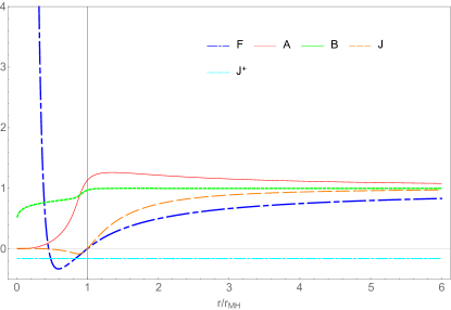
Figure 1: The solution for $c_{1}=0.051$, $c_{2}=0.116$, $c_{3}=-c_{1}$ and $c_{4}=0$, first considered numerically in Eling2006-2 . There are an outer and inner MHs, at which $F$ vanishes. But, $J$ does not cross the constant line of $J^{+}$, so that a S0H is absent. This graph is the same as the one given in Eling2006-2 (up to the numerical errors).

III.2 Exact Solutions with $c_{14}=c_{13}=0$

From Eqs.(2.15) - (2.20) we can see that the choice $c_{14}=c_{13}=0$ satisfies these constraints, provided that $c_{2}$ satisfies the condition ,

$$0\lesssim c_{2}\lesssim 0.095.$$ (3.20)

Then, we find that Eqs.(3.5)-(3.6) now reduce to

$$F^{\prime\prime} = -\frac{2}{r}F^{\prime}+\frac{c_{2}\hat{\cal{F}}(r)}{4r^{2}A^{4}},$$ (3.21)

$$A^{\prime\prime} = \frac{2}{r^{2}(A+A^{3}F)}\Big{[}r^{2}(A^{\prime})^{2}-rAA^{\prime}-A^{2}$$ (3.22)

$$-rA^{3}A^{\prime}(F+rF^{\prime})+A^{4}F\Big{]}$$

$$-\frac{c_{2}\hat{\cal{F}}(r)}{4r^{2}(A+A^{3}F)},$$

where

$$\hat{\cal{F}}(r)\equiv\left[rA^{\prime}-2A+rA^{2}A^{\prime}F+A^{3}\left(2F+rF^{\prime}\right)\right]^{2}.~{}~{}~{}~{}$$ (3.23)

Combining Eqs.(3.21) and (3.22), we find the following equation,

$$W^{\prime\prime}+{W^{\prime}}^{2}+\frac{2}{r}W^{\prime}-\frac{2}{r^{2}}=0,$$ (3.24)

where

$$W \equiv \ln\left(\frac{1-FA^{2}}{A}\right).$$ (3.25)

Eq.(3.24) has the general solution,

$$W=\ln w_{2}+\ln\left(\frac{1+w_{1}r^{3}}{r^{2}}\right),$$ (3.26)

where $w_{1}$ and $w_{2}$ are two integration constants. Then, the combination of Eqs.(3.25) and (3.26) yields,

$$F(r) = \frac{1}{A^{2}}-\frac{w_{2}}{A}\left(\frac{1}{r^{2}}+w_{1}r\right).$$ (3.27)

Substituting Eq.(3.27) into Eq.(3.21), we find

$$F^{\prime\prime} = -\frac{2}{r}F^{\prime}+F_{0},$$ (3.28)

where $F_{0}\equiv 9c_{2}w_{1}^{2}w_{2}^{2}/4$. Integrating Eq.(3.28), we find

$$F(r) = F_{2}\left(1-\frac{2m}{r}\right)+\frac{F_{0}}{6}r^{2},$$ (3.29)

where $m$ and $F_{2}$ are two other integration constants. On the other hand, from Eq.(3.27), we find that

$$A(r) = -\frac{w_{2}}{2F}\Bigg{[}\left(\frac{1}{r^{2}}+w_{1}r\right)$$ (3.30)

$$\left.\pm\sqrt{\frac{4F}{w_{2}^{2}}+\left(\frac{1}{r^{2}}+w_{1}r\right)^{2}}\right].$$

Substituting the above expressions for $A$ and $F$ into the constraint (3.11), we find that

$$B = \sqrt{F_{2}}.$$ (3.31)

Note that the above solution is asymptotically flat only when $w_{1}=0$, for which we have

$$F(r) = F_{2}\left(1-\frac{2m}{r}\right),\quad B(r)=\sqrt{F_{2}},$$

$$A(r) = -\frac{w_{2}}{2F}\left(\frac{1}{r^{2}}\pm\sqrt{\frac{4F}{w_{2}^{2}}+\frac{1}{r^{4}}}\right).$$ (3.32)

Using the gauge residual $v^{\prime}=C_{0}v+C_{1}$ of the metric (3.1), without loss of the generality, we can always set $F_{2}=1$, so the corresponding metric takes the precise form of the Schwarzschild solution,

$$ds^{2}=-\left(1-\frac{2m}{r}\right)dv^{2}+2dvdr+r^{2}d\Omega^{2},$$ (3.33)

while the aether field is given by

$$A(r) = -\frac{w_{2}\pm\sqrt{w_{2}^{2}+4r^{3}(r-2m)}}{2r(r-2m)}.~{}~{}~{}~{}~{}$$ (3.34)

It is remarkable to note that now the aether field has no contribution to the spacetime geometry, although it does feel the gravitational field, as it can be seen from Eq.(3.34).

It should be also noted that Eqs.(3.33) and (3.34) were a particular case of the solutions first found in Per12 for the case $c_{14}=0$ by further setting $c_{13}=0$. But, the general solutions given by Eqs.(3.29) - (3.31) are new, as far as we know.

III.3 Field Equations for $\tilde{g}_{\mu\nu}$ and $\tilde{u}^{\mu}$

Note that, instead of solving the three independent equations directly for $A$, $B$ and $F$, we shall first solve the corresponding three equations for $\tilde{A}$, $\tilde{B}$ and $\tilde{F}$, by taking the advantage of the field redefinitions introduced in the last section, and then obtain the functions $A$, $B$ and $F$ by the inverse transformations of Eqs.(III.3) and (3.41) to be given below. This will considerably simplify mathematically the problem of solving such complicated equations.

To this goal, let us first note that, with the filed redefinitions (II.1), the line element corresponding to $\hat{g}_{\mu\nu}$ in the coordinates ($v,r,\theta,\phi$), takes the form,

$$d\hat{s}^{2} \equiv \hat{g}_{\mu\nu}dx^{\mu}dx^{\nu}$$ (3.35)

$$= -\left[F+\frac{(\sigma-1)\left(A^{2}F+1\right)^{2}}{4A^{2}}\right]dv^{2}$$

$$+2\left[B+\frac{1}{2}(\sigma-1)B\left(A^{2}F+1\right)\right]dvdr$$

$$-(\sigma-1)A^{2}B^{2}dr^{2}+r^{2}d\Omega^{2}.$$

To bring the above expression into the standard EF form, we first make the coordinate transformation,

$$\tilde{v}=C_{0}v-C(r),$$ (3.36)

where $C_{0}$ is an arbitrary real constant, and $C(r)$ is a function of $r$. Then, choosing $C(r)$ so that

$$\frac{dC(r)}{dr} = \frac{2C_{0}A^{2}B\left(\sqrt{\sigma}-1\right)}{J\left(\sqrt{\sigma}-1\right)+(\sqrt{\sigma}+1)},$$ (3.37)

we find that in the coordinates ${\tilde{x}}^{\mu}=(\tilde{v},r,\theta,\phi)$ the line element (3.35) takes the form,

$$d\hat{s}^{2} \equiv \hat{g}_{\mu\nu}dx^{\mu}dx^{\nu}=\tilde{g}_{\mu\nu}d\tilde{x}^{\mu}d\tilde{x}^{\nu}$$ (3.38)

$$= -\tilde{F}(r)d\tilde{v}^{2}+2\tilde{B}(r)d\tilde{v}dr+r^{2}d\Omega^{2},$$

where

$${\tilde{F}} = \frac{J^{2}(\sigma-1)+2J(\sigma+1)+(\sigma-1)}{4C_{0}^{2}A^{2}},$$

$${\tilde{B}} = \frac{\sqrt{\sigma}B}{C_{0}}.$$ (3.39)

On the other hand, in terms of the coordinates $\tilde{x}^{\mu}$, the aether four-velocity is given by

$$\hat{u}^{\alpha}\frac{\partial}{\partial{x}^{\alpha}}=\tilde{u}^{\alpha}\frac{\partial}{\partial\tilde{x}^{\alpha}}=\tilde{A}(r)\partial_{\tilde{v}}-\frac{1-\tilde{F}(r)\tilde{A}^{2}(r)}{2\tilde{B}(r)\tilde{A}(r)}\partial_{r},~{}~{}~{}~{}~{}~{}$$ (3.40)

where

$${\tilde{A}}=\frac{2C_{0}A}{J\left(\sqrt{\sigma}-1\right)+(\sqrt{\sigma}+1)},$$ (3.41)

which satisfies the constraint $\tilde{u}^{\alpha}\tilde{u}^{\beta}\tilde{g}_{\alpha\beta}=-1$, with

$$\tilde{g}_{\mu\nu}\equiv\frac{\partial x^{\alpha}}{\partial\tilde{x}^{\mu}}\frac{\partial x^{\beta}}{\partial\tilde{x}^{\nu}}\hat{g}_{\alpha\beta},\quad\tilde{u}_{\mu}\equiv\frac{\partial x^{\alpha}}{\partial\tilde{x}^{\mu}}\hat{u}_{\alpha}.$$ (3.42)

It should be noted that the metric (3.38) still has the gauge residual,

$$\tilde{\tilde{v}}=C_{1}\tilde{v}+C_{2},$$ (3.43)

where $C_{1}$ and $C_{2}$ are two arbitrary constants, which will keep the line element in the same form, after the rescaling,

$$\tilde{\tilde{F}}=\frac{\tilde{F}}{C_{1}^{2}},\quad\tilde{\tilde{B}}=\frac{\tilde{B}}{C_{1}}.$$ (3.44)

Later we shall use this gauge freedom to fix one of the initial conditions.

In the rest of this paper, we always refer $\left(\tilde{g}_{\mu\nu},\tilde{u}^{\alpha}\right)$ as the field obtained by the field redefinitions. The latter is related to $\left(\hat{g}_{\mu\nu},\hat{u}^{\alpha}\right)$ via the inverse coordinate transformations of Eq.(3.42). Then, the Einstein-aether field equations for $\left(\tilde{g}_{\mu\nu},\tilde{u}^{\alpha}\right)$ will take the same forms as those given by Eqs.(2.29) - (2.31), but now in terms of $\left(\tilde{g}_{\mu\nu},\tilde{u}^{\alpha},\tilde{c}_{i}\right)$ in the coordinates $\tilde{x}^{\mu}$, where $\tilde{c}_{i}\equiv\hat{c}_{i}$.

On the other hand, since the metric (3.38) for $\tilde{g}_{\mu\nu}$ takes the same form as the metric (3.1) for $g_{\mu\nu}$, and so does the aether field (3.40) for $\tilde{u}^{\mu}$ as the one (3.2) for $u^{\mu}$, it is not difficult to see that the field equations for $\tilde{F}(r),\;\tilde{A}(r)$ and $\tilde{B}(r)$ will be given precisely by Eqs.(3.5) - (3.10), if we simply make the following replacement,

$$\left(F,A,B,c_{i}\right)\rightarrow\left(\tilde{F},\tilde{A},\tilde{B},\tilde{c}_{i}\right).$$ (3.45)

As a result, we have

$$\tilde{F}^{\prime\prime} = \tilde{\mathcal{F}}\left(\tilde{A},\tilde{A}^{\prime},\tilde{F},\tilde{F}^{\prime},r,\tilde{c}_{i}\right)$$ (3.46)

$$= \frac{1}{2r^{2}\tilde{A}^{4}\tilde{\cal{D}}}\Big{[}\tilde{f}_{0}+\tilde{f}_{1}\tilde{F}+\tilde{f}_{2}\tilde{F}^{2}+\tilde{f}_{3}\tilde{F}^{3}$$

$$~{}~{}~{}~{}~{}~{}~{}~{}~{}~{}~{}~{}+\tilde{f}_{4}\tilde{F}^{4}\Big{]},$$

$$\tilde{A}^{\prime\prime} = \tilde{\mathcal{A}}\left(\tilde{A},\tilde{A}^{\prime},\tilde{F},\tilde{F}^{\prime},r,\tilde{c}_{i}\right)$$ (3.47)

$$= \frac{1}{2r^{2}\tilde{A}^{2}\tilde{\cal{D}}}\Big{[}\tilde{a}_{0}+\tilde{a}_{1}\tilde{F}+\tilde{a}_{2}\tilde{F}^{2}+\tilde{a}_{3}\tilde{F}^{3}\Big{]},$$

$$\frac{\tilde{B}^{\prime}}{\tilde{B}} = \tilde{\mathcal{B}}\left(\tilde{A},\tilde{A}^{\prime},\tilde{F},\tilde{F}^{\prime},r,\tilde{c}_{i}\right)$$ (3.48)

$$= \frac{1}{2r\tilde{A}^{2}\tilde{\cal{D}}}\Big{[}\tilde{b}_{0}+\tilde{b}_{1}\tilde{F}+\tilde{b}_{2}\tilde{F}^{2}\Big{]},$$

and

$${\tilde{C}}^{\tilde{v}}\equiv\tilde{n}_{0}+\tilde{n}_{1}\tilde{F}+\tilde{n}_{2}\tilde{F}^{2}=0,$$ (3.49)

where

$$\tilde{\cal{D}}(r) \equiv \tilde{d}_{-}\left(\tilde{J}^{2}(r)+1\right)+{2}\tilde{d}_{+}\tilde{J}(r),$$

$$\tilde{J}(r) \equiv \tilde{F}(r)\tilde{A}^{2}(r),$$

$$\tilde{d}_{\pm} \equiv (\tilde{c}_{S}^{2}\pm 1)\tilde{c}_{14}(1-\tilde{c}_{13})(2+\tilde{c}_{13}+3\tilde{c}_{2}).$$ (3.50)

The coefficients $\tilde{f}_{n},\;\tilde{a}_{n},\;\tilde{b}_{n}$ and $\tilde{n}_{n}$ are given by $f_{n},\;a_{n},\;b_{n}$ and $n_{n}$ after the replacement (3.45) is carried out.

Then, the metric and spin-0 horizons for $\tilde{g}_{\mu\nu}$ are given, respectively, by

$$\tilde{g}_{\alpha\beta}\tilde{N}^{\alpha}\tilde{N}^{\beta}=0,$$ (3.51)

$$\tilde{g}^{(S)}_{\alpha\beta}\tilde{N}^{\alpha}\tilde{N}^{\beta}=0,$$ (3.52)

where $\tilde{N}_{\alpha}=(\partial x^{\mu}/\partial\tilde{x}^{\alpha})N_{\mu}={\delta^{r}_{\tilde{\alpha}}=\delta^{r}_{\alpha}}$ and

$$\tilde{g}^{(S)}_{\alpha\beta}\equiv\tilde{g}_{\alpha\beta}-\left(\tilde{c}_{S}^{2}-1\right)\tilde{u}_{\alpha}\tilde{u}_{\beta}.$$ (3.53)

In terms of $\tilde{F}$ and $\tilde{A}$, Eqs.(3.51) and (3.52) becomes,

$$\tilde{F}(\tilde{r}_{MH})=0,$$ (3.54)

$$\left(\tilde{c}_{S}^{2}-1\right)\left(\tilde{J}(\tilde{r}_{S0H})^{2}+1\right)+2\left(\tilde{c}_{S}^{2}+1\right)\tilde{J}(\tilde{r}_{S0H})=0,$$

where $r=\tilde{r}_{MH}$ and $r=\tilde{r}_{S0H}$ are respectively the locations of the metric and spin-0 horizons for the metric $\tilde{g}_{\mu\nu}$. Similarly, at $r=\tilde{r}_{S0H}$ we have

$$\tilde{\cal{D}}(\tilde{r}_{S0H})=0.$$ (3.56)

Comparing the field equations given in this subsection with the corresponding ones given in the last subsection, we see that we can get one set from the other simply by the replacement (3.45).

In addition, in terms of $\hat{g}_{\alpha\beta}$ and $N_{\alpha}$, Eqs.(3.51) and (3.52) reduce, respectively, to

$$\hat{g}_{\alpha\beta}N^{\alpha}N^{\beta}=0,$$ (3.57)

$$\hat{g}^{(S)}_{\alpha\beta}N^{\alpha}N^{\beta}=0.$$ (3.58)

Since $\tilde{r}=r$, we find that

$$\tilde{r}_{MH}=\hat{r}_{MH},\quad\tilde{r}_{S0H}=\hat{r}_{S0H},$$ (3.59)

where $\tilde{r}_{MH}$ and $\tilde{r}_{S0H}$ ($\hat{r}_{MH},\hat{r}_{S0H}$) are the locations of the metric and spin-0 horizons of the metric $\tilde{g}_{\alpha\beta}$ ($\hat{g}_{\alpha\beta}$). The above analysis shows that these horizons determined by $\tilde{g}_{\alpha\beta}$ are precisely equal to those determined by $\hat{g}_{\alpha\beta}$.

III.4 $\sigma=c_{S}^{2}$

To solve Eqs.(3.46) - (3.49), we take the advantage of the choice $\sigma=c_{S}^{2}$, so that the speed of the spin-0 mode of the metric $\hat{g}_{\mu\nu}$ becomes unity, i.e., $\hat{c}_{S}=1$. Since $\tilde{c}_{i}=\hat{c}_{i}$, we also have $\tilde{c}_{S}=\hat{c}_{S}=1$. Then, from Eq.(I) we find that this leads to,

$$\tilde{c}_{2}=\frac{2\tilde{c}_{14}-2\tilde{c}_{13}-\tilde{c}_{13}^{2}\tilde{c}_{14}}{2-4\tilde{c}_{14}+3\tilde{c}_{13}\tilde{c}_{14}}.$$ (3.60)

For such a choice, from Eq.(III.3) we find that $\tilde{d}_{-}=0$, and

$$\tilde{\cal{D}}(r)={2}\tilde{d}_{+}\tilde{J}(r)={2}\tilde{d}_{+}\tilde{A}^{2}(r)\tilde{F}(r).$$ (3.61)

Then, Eq.(3.56) yields $\tilde{F}(\tilde{r}_{S0H})=0$, since $\tilde{A}\not=0$, which also represents the location of the MH, defined by Eq.(3.54). Therefore, for the choice $\sigma=c_{S}^{2}$ the MH coincides with the S0H for the effective metric $\tilde{g}_{\mu\nu}$, that is,

$$\tilde{r}_{MH}=\tilde{r}_{S0H},\;\left(\sigma=c_{S}^{2}\right).$$ (3.62)

As shown below, this will significantly simplify our computational labor. In particular, if we choose this surface as our initial moment, it will reduce the phase space of initial data from 4 dimensions to one dimension only.

For $\tilde{c}_{S}=1$, Eqs.(3.46)-(3.49) reduce to,

$$\tilde{F}^{\prime\prime}=\frac{1}{{4}\tilde{d}_{+}r^{2}\tilde{A}^{6}}\left(\frac{\tilde{f}_{0}}{\tilde{F}}+\tilde{f}_{1}+\tilde{f}_{2}\tilde{F}+\tilde{f}_{3}\tilde{F}^{2}\right.$$

$$~{}~{}~{}~{}~{}~{}~{}~{}~{}~{}~{}~{}~{}~{}~{}~{}~{}~{}~{}~{}~{}~{}~{}~{}\left.+\tilde{f}_{4}\tilde{F}^{3}\right),$$ (3.63)

$$\tilde{A}^{\prime\prime}=\frac{1}{{4}\tilde{d}_{+}r^{2}\tilde{A}^{4}}\left(\frac{\tilde{a}_{0}}{\tilde{F}}+\tilde{a}_{1}+\tilde{a}_{2}\tilde{F}+\tilde{a}_{3}\tilde{F}^{2}\right),~{}~{}~{}$$ (3.64)

$$\frac{\tilde{B}^{\prime}}{\tilde{B}}=\frac{1}{{4}\tilde{d}_{+}r\tilde{A}^{4}}\left(\frac{\tilde{b}_{0}}{\tilde{F}}+\tilde{b}_{1}+\tilde{b}_{2}\tilde{F}\right),$$ (3.65)

$$\tilde{n}_{0}+\tilde{n}_{1}\tilde{F}+\tilde{n}_{2}\tilde{F}^{2}=0.$$ (3.66)

As shown previously, among these four equations, only three of them are independent, and our strategy in this paper is to take Eqs.(III.4), (3.64) and (3.66) as the three independent equations. The advantage of this approach is that Eqs.(III.4), (3.64) are independent of $\tilde{B}(r)$, and Eq.(3.66) is a quadratic polynomial of $\tilde{B}(r)$. So, we can solve Eqs.(III.4), (3.64) as the initial value problem first to find $\tilde{F}(r)$ and $\tilde{A}(r)$, and then insert them into Eq.(3.66) to obtain directly $\tilde{B}(r)$, as explicitly given by Eq.(3.11), after taking the replacement (3.45) and the choice of $\tilde{c}_{2}$ of Eq.(3.60) into account.

From Eqs.(III.4) and (3.64) we can see that they become singular at $r=\tilde{r}_{S0H}$ (Recall $\tilde{F}(\tilde{r}_{S0H})=0$), unless $\tilde{f}_{0}(\tilde{r}_{S0H})=\tilde{a}_{0}(\tilde{r}_{S0H})=0$. As can be seen from the expressions of $f_{0}(r),\;a_{0}(r)$ given in Appendix A, $\tilde{f}_{0}(\tilde{r}_{S0H})=\tilde{a}_{0}(\tilde{r}_{S0H})=0$ imply $\tilde{b}_{0}(\tilde{r}_{S0H})=0$. Therefore, to have the field equations regular across the S0H, we must require $\tilde{b}_{0}(\tilde{r}_{S0H})=0$. It is interesting that this is also the condition for Eq.(3.65) to be non-singular across the S0H. In addition, using the gauge residual (3.43), we shall set $\tilde{B}_{H}=1$, so Eq.(3.66) [which can be written in the form of Eq.(3.11), after the replacement (3.45)] will provide a constraint among the initial values of $\tilde{F}^{\prime}_{H}$, $\tilde{A}_{H}$ and $\tilde{A}^{\prime}_{H}$, where $\tilde{F}^{\prime}_{H}\equiv\tilde{F}^{\prime}(\tilde{r}_{S0H})$ and so on. In summary, on the S0H we have the following

$$\tilde{F}_{H}=0,$$ (3.67)

$$\tilde{b}_{0}\left(\tilde{A}_{H},\tilde{A}^{\prime}_{H},\tilde{F}^{\prime}_{H},\tilde{r}_{S0H}\right)=0,$$ (3.68)

$$\tilde{B}_{H}=1.$$ (3.69)

From the expression for $\tilde{b}_{0}$ given in Appendix A, we can see that Eq.(3.68) is quadratic in $\tilde{A}^{\prime}_{H}$, and solving it on the S0H, in general we obtain two solutions,

$$\tilde{A^{\prime}}^{\pm}_{H}=\tilde{A^{\prime}}^{\pm}_{H}\left(\tilde{A}_{H},\tilde{F}^{\prime}_{H},\tilde{r}_{S0H}\right).$$ (3.70)

Then, inserting it, together with Eqs.(3.67) and (3.69), into Eq.(3.10), we get

$$\tilde{n}^{\pm}_{0}\left(\tilde{A}_{H},\tilde{F}^{\prime}_{H},\tilde{r}_{S0H}\right)=0,$$ (3.71)

where the “$\pm$” signs correspond to the choices of $\tilde{A^{\prime}}_{H}=\tilde{A^{\prime}}^{\pm}_{H}$. In general, Eq.(3.71) is a fourth-order polynomial of $\tilde{F}^{\prime}_{H}$, so it normally has four roots, denoted as

$$\tilde{F^{\prime}}^{(\pm,n)}_{H}=\tilde{F^{\prime}}^{(\pm,n)}_{H}\left(\tilde{A}_{H},\tilde{r}_{S0H}\right),$$ (3.72)

where $n=1,2,3,4$. For each given $\tilde{F^{\prime}}^{(\pm,n)}_{H}$, substituting it into Eq.(3.70) we find a corresponding $\tilde{A^{\prime}}^{(\pm,n)}_{H}$, given by

$$\tilde{A^{\prime}}^{(\pm,n)}_{H}=\tilde{A^{\prime}}^{(\pm,n)}_{H}\left(\tilde{A}_{H},\tilde{r}_{S0H}\right).$$ (3.73)

Thus, once $\tilde{A}_{H}$ and $\tilde{r}_{S0H}$ are given, the quantities $\tilde{F^{\prime}}^{(\pm,n)}_{H}$ and $\tilde{A^{\prime}}^{(\pm,n)}_{H}$ are uniquely determined from Eqs.(3.72) and (3.73). For each set of ($\tilde{A}_{H},\tilde{r}_{S0H}$), in general there are eight sets of $\left(\tilde{A}^{\prime}_{H},\tilde{F}^{\prime}_{H}\right)$.

If we choose $r=\tilde{r}_{S0H}$ as the initial moment, such obtained $\left(\tilde{A}^{\prime}_{H},\tilde{F}^{\prime}_{H}\right)$, together with $\tilde{F}_{H}=0$, and a proper choice of $\tilde{A}_{H}$, can be considered as the initial conditions for the differential equations (III.4) and (3.64).

However, it is unclear which one(s) of these eight sets of initial conditions will lead to asymptotically flat solutions, except that the one with $\tilde{F}^{\prime}_{H}<0$, which can be discarded immediately, as it would lead to $\tilde{F}=0$ at some radius $r>\tilde{r}_{S0H}$, which is inconsistent with our assumption that $r=\tilde{r}_{S0H}$ is the location of the S0H Enrico11 . So, in general what one needs to do is to try all the possibilities.

Therefore, if we choose $r=\tilde{r}_{S0H}$ as the initial moment, the four-dimensional phase space of the initial conditions, $\left(\tilde{F}_{H},\tilde{F}^{\prime}_{H},\tilde{A}_{H},\tilde{A}^{\prime}_{H}\right)$, reduces to one-dimensional, spanned by $\tilde{A}_{H}$ only.

In the following, we shall show further that $\tilde{r}_{S0H}$ can be chosen arbitrarily. In fact, introducing the dimensionless quantity, $\xi\equiv\tilde{r}_{S0H}/r$, we find that Eqs. (III.4) - (3.65) and (3.49) can be written in the forms,

$$\frac{d^{2}\tilde{F}(\xi)}{d\xi^{2}}={\cal{G}}_{1}\left(\xi,\tilde{c}_{i}\right),$$ (3.74)

$$\frac{d^{2}\tilde{A}(\xi)}{d\xi^{2}}={\cal{G}}_{2}\left(\xi,\tilde{c}_{i}\right),$$ (3.75)

$$\frac{1}{\tilde{B}(\xi)}\frac{d\tilde{B}(\xi)}{d\xi}={\cal{G}}_{3}\left(\xi,\tilde{c}_{i}\right),$$ (3.76)

$$C^{\tilde{v}}\left(\tilde{A}(\xi),\tilde{A}^{\prime}(\xi),\tilde{F}(\xi),\tilde{F}^{\prime}(\xi),\tilde{B}(\xi),\xi,\tilde{c}_{i}\right)=0,~{}~{}~{}~{}~{}$$ (3.77)

where ${\cal{G}}_{i}$’s are all independent of $\tilde{r}_{S0H}$, $C^{\tilde{v}}\equiv r_{S0H}^{2}\tilde{C}^{\tilde{v}}$, and the primes in the last equation stand for the derivatives respect to $\xi$. Therefore, Eqs.(3.74)-(3.77), or equivalently, Eqs.(3.46)-(3.49), are scaling-invariant and independent of $\tilde{r}_{S0H}$. Thus, without loss of the generality, we can always set

$$\tilde{r}_{S0H}=1,$$ (3.78)

which does not affect Eqs.(3.74) - (3.77), and also explains the reason why in Eling2006-2 ; Enrico11 the authors set $\tilde{r}_{S0H}=1$ directly. At the same time, it should be noted that once $\tilde{r}_{S0H}=1$ is taken, it implies that the unit of length is fixed. For instance, if we have a BH with $\tilde{r}_{S0H}=1$ km, then setting $\tilde{r}_{S0H}=1$ means the unit of length is in km.

Once $\tilde{A}_{H}$ is chosen, we can integrate Eqs.(3.74) and (3.75) in both directions to find $\tilde{F}(\xi)$ and $\tilde{A}(\xi)$, one is toward the center, $\xi=\tilde{r}_{S0H}/r=\infty$, in which we have $\xi\in[1,\infty)$, and the other is toward infinity, $\xi=\tilde{r}_{S0H}/r=0$, in which we have $\xi\in(0,1]$. Then, from Eq.(3.11) we can find $\tilde{B}(\xi)$ uniquely, after the replacement of Eq.(3.45). Again, to have a proper asymptotical behavior of $\tilde{B}(r)$, the “+” sign will be chosen.

At the spatial infinity $\xi=\tilde{r}_{S0H}/r\rightarrow 0$, we require that the spacetime be asymptotically flat, that is Eling2006-2 ; Enrico11 ,

$$\tilde{F}(\xi) = 1+\tilde{F}_{1}\xi+\frac{1}{48}\tilde{c}_{14}\tilde{F}_{1}^{3}\xi^{3}+\cdots,$$

$$\tilde{A}(\xi) = 1-\frac{1}{2}\tilde{F}_{1}\xi+\frac{1}{2}\tilde{A}_{2}\xi^{2}-\Bigg{(}\frac{1}{96}\tilde{c}_{14}\tilde{F}_{1}^{3}$$

$$-\frac{1}{16}\tilde{F}_{1}^{3}+{\frac{1}{2}\tilde{F}_{1}\tilde{A}_{2}}\Bigg{)}\xi^{3}+\cdots,$$

$$\tilde{B}(\xi) = 1+\frac{1}{16}\tilde{c}_{14}\tilde{F}_{1}^{2}\xi^{2}-\frac{1}{12}\tilde{c}_{14}\tilde{F}_{1}^{3}\xi^{3}+\cdots,$$ (3.79)

where $\tilde{F}_{1}\equiv\tilde{F}^{\prime}(\xi=0)$ and $\tilde{A}_{2}\equiv\tilde{A}^{\prime\prime}(\xi=0)$.

It should be noted that the Minkowski spacetime is given by

$$\tilde{F}=\tilde{F}_{M},~{}~{}\quad\tilde{A}=\frac{1}{\sqrt{\tilde{F}_{M}}},~{}~{}\quad\tilde{B}=\sqrt{\tilde{F}_{M}},~{}~{}~{}~{}~{}~{}~{}$$ (3.80)

where $\tilde{F}_{M}$ is a positive otherwise arbitrary constant. Therefore, in the asymptotical expansions of Eq.(III.4), we had set $\tilde{F}_{M}=1$ at the zeroth order of $\xi$. However, the initial conditions imposed at $r=\tilde{r}_{S0H}$ given above usually leads to $\tilde{F}_{M}\not=1$, even for spacetimes that are asymptotically flat. Therefore, we need first to use the gauge residual (3.43) to bring $\tilde{F}(\xi=0)=\tilde{A}(\xi=0)=\tilde{B}(\xi=0)=1$, before using Eq.(III.4) to calculate the constants $\tilde{A}_{2}$ and $\tilde{F}_{1}$.

From the above analysis we can see that finding spherically symmetric solutions of the $\ae$-theory now reduces to finding the initial condition $\tilde{A}_{H}$ that leads to the asymptotical behavior (III.4), for a given set of $c_{i}$’s.

Before proceeding to the next section, we would like to recall that when $\sigma=c_{S}^{2}$, we have $g^{(S)}_{\alpha\beta}=\hat{g}_{\alpha\beta}$, as shown by Eq.(2.35). That is, the S0H for the metric $g_{\alpha\beta}$ now coincides with the MH of $\hat{g}_{\alpha\beta}$. With this same very choice, $\sigma=c_{S}^{2}$, the MH for $\hat{g}_{\alpha\beta}$ also coincides with its S0H. Thus, we have

$$r_{S0H}=\hat{r}_{S0H}=\hat{r}_{MH}=\tilde{r}_{S0H}=\tilde{r}_{MH}\equiv r_{H},\;\left(\sigma=c_{S}^{2}\right).$$

It must be noted that $r_{H}$ defined in the last step denotes the location of the S0H of $g_{\alpha\beta}$, which is usually different from its MH, defined by

$$\left.g_{\alpha\beta}N^{\alpha}N^{\beta}\right|_{r=r_{MH}}=0,$$ (3.82)

since in general we have $c_{S}\not=1$, so $g^{(S)}_{\alpha\beta}\equiv g_{\alpha\beta}-\left(c_{S}^{2}-1\right)u_{\alpha}u_{\beta}\not=g_{\alpha\beta}$. As a result, we have $r_{MH}\not=r_{S0H}$ for $c_{S}\not=1$.

However, it is worth emphasizing again that, for the choice $\sigma=c_{S}^{2}$ we have $\tilde{c}_{S}=\hat{c}_{S}=1$, so the metric and spin-0 horizons of both $\hat{g}_{\alpha\beta}$ and $\tilde{g}_{\alpha\beta}$ all coincide, and are given by the same $r_{H}$, as explicitly shown by Eq.(III.4). More importantly, it is also the location of the S0Hs of the metric $g_{\alpha\beta}$.

IV Numerical Setup and Results

IV.1 General Steps

It is difficult to find analytical solutions to Eqs.(3.74)-(3.77). Thus, in this paper we are going to solve them numerically, using the shooting method, with the asymptotical conditions (III.4). In particular, our strategy is the following:

(i) Choose a set of physical $c_{i}$’s satisfying the constraints (2.16)-(2.20), and then calculate the corresponding $\tilde{c}_{i}$’s with $\sigma={c}_{S}^{2}$.

(ii) Assume that for such chosen $c_{i}$’s the corresponding solution possesses a S0H located at $r=r_{H}$, and then follow the analysis given in the last section to impose the conditions $\tilde{F}_{H}=0$ and $\tilde{B}_{H}=1$.

(iii) Choose a test value for $\tilde{A}_{H}$, and then solve Eq.(3.68) for $\tilde{A}^{\prime}_{H}$ in terms of $\tilde{F}^{\prime}_{H}$ and $\tilde{A}_{H}$, i.e., $\tilde{A}^{\prime}_{H}=\tilde{A}^{\prime}_{H}(\tilde{F}^{\prime}_{H},\tilde{A}_{H})$.

(iv) Substitute $\tilde{A}^{\prime}_{H}$ into Eq.(3.71) to obtain a quartic equation for $\tilde{F}^{\prime}_{H}$ and then solve it to find $\tilde{F}^{\prime}_{H}$.

(v) With the initial conditions $\{\tilde{F}_{H},\tilde{A}_{H},\tilde{F}^{\prime}_{H},\tilde{A}^{\prime}_{H}\}$, integrate Eqs.(3.74) and (3.75) from $\xi=1$ to $\xi=0$.

However, since the field equations are singular at $\xi=1$, we will actually integrate these equations from $\xi=1-\epsilon$ to $\xi\simeq 0$, where $\epsilon$ is a very small quantity. To obtain the values of $\digamma(\xi)$ at $\xi=1-\epsilon$, we first Taylor expand them in the form,

$${\digamma(1-\epsilon)=\sum_{k=0}^{2}\frac{\digamma^{(k)}|_{\xi=1}}{k!}(-1)^{k}\epsilon^{k}+{\cal{O}}\left(\epsilon^{3}\right),}$$ (4.1)

where $\digamma\equiv\left\{\tilde{A},\tilde{A}^{\prime},\tilde{F},\tilde{F}^{\prime}\right\}$ and $\digamma^{(k)}\equiv d^{k}\digamma/d\xi^{k}$. For each $\digamma$, we shall expand it to the second order of $\epsilon$, so the errors are of the order $\epsilon^{3}$. Thus, if we choose $\epsilon=10^{-14}$, the errors in the initial conditions $\digamma(1-\epsilon)$ is of the order $10^{-42}$. For $\digamma=\tilde{A},\;\tilde{F}$, we already obtained $\digamma(1)$ and $\digamma^{\prime}(1)$ from the initial conditions. In these cases, to get $\tilde{A}^{\prime\prime}(1)$ and $\tilde{F}^{\prime\prime}(1)$, we use the field equations (3.74) and (3.75) and L’Hospital’s rule. On the other hand, for $\digamma=\tilde{A}^{\prime}$, expanding it to the second order of $\epsilon$, we have

$$\tilde{A}^{\prime}(1-\epsilon)=\tilde{A}^{\prime}(1)-\tilde{A}^{\prime\prime}(1)\epsilon+\frac{1}{2}\tilde{A}^{(3)}(1)\epsilon^{2}+{\cal{O}}\left(\epsilon^{3}\right),$$ (4.2)

where $\tilde{A}^{(3)}(1)\equiv\left.d^{3}\tilde{A}(\xi)/d\xi^{3}\right|_{\xi=1}$ can be obtained by first taking the derivative of Eq.(3.75) and then taking the limit $\xi\rightarrow 1$, as now we have already known $\tilde{A}(1),\tilde{A}^{\prime}(1),\tilde{A}^{\prime\prime}(1),\tilde{F}(1),\tilde{F}^{\prime}(1)$ and $\tilde{F}^{\prime\prime}(1)$. Similarly, for $\digamma=\tilde{F}^{\prime}$, from Eq.(3.74) we can find $\tilde{F}^{(3)}(1)$.

(vi) Repeat (iii)-(v) until a numerical solution matched to Eq.(III.4) is obtained, by choosing different values of $\tilde{A}_{H}$ with a bisectional search. Clearly, once such a value of $\tilde{A}_{H}$ is found, it means that we obtain numerically an asymptotically flat solution of the Einstein-aether field equations outside the S0H. Note that, to guarantee that Eq.(III.4) is satisfied, the normalization of $\{\tilde{F},\tilde{A},\tilde{B}\}$ need to be done according to Eq.(3.80), by using the remaining gauge residual of Eq.(3.43).

(vii) To obtain the solution in the internal region $\xi\in(1,\infty)$, we simply integrate Eqs.(3.74) and (3.75) from $\xi=1$ to $\xi\to\infty$ with the same value of $\tilde{A}_{H}$ found in the last step. As in the region $\xi\in(0,1)$, we can’t really set the “initial” conditions precisely at $\xi=1$. Instead, we will integrate them from $\xi=1+\epsilon$ to $\xi=\xi_{\infty}\gg 1$. The initial values at $\xi=1+\epsilon$ can be obtained by following what we did in Step (v), that is, Taylor expand $\digamma(\xi)$ at $\xi=1+\epsilon$, and then use the field equations to get all the quantities up to the third-order of $\epsilon$.

(viii) Matching the results obtained from steps (vi) and (vii) together, we finally obtain a solution of $\{\tilde{F}(\xi),\tilde{A}(\xi)\}$ on the whole spacetime $\xi\in(0,\infty)$ (or $r\in(0,\infty)$).

(ix) Once $\tilde{F}$ and $\tilde{A}$ are known, from Eq.(3.11), we can calculate $\tilde{B}$, so that an asymptotically flat black hole solution for $\{\tilde{A},\tilde{B},\tilde{F}\}$ is finally obtained over the whole space $r\in(0,\infty)$.

Before proceeding to the next subsection to consider the physically allowed region of the parameter space of $c_{i}$’s, let us first reproduce the results presented in Table I of Enrico11 , in order to check our numerical code, although all these choices have been ruled out currently by observations OMW18 . To see this explicitly, let us first note that the parameters chosen in Eling2006-2 ; Enrico11 correspond to

$$\hat{c}_{2}=-\frac{\hat{c}_{1}^{3}}{3\hat{c}_{1}^{2}-4\hat{c}_{1}+2},\quad\hat{c}_{3}=0=\hat{c}_{4}=0,$$ (4.3)

so that now only $\hat{c}_{1}$ is a free parameter. With this choice of $\hat{c}_{i}$’s, the corresponding $c_{i}$’s can be obtained from Eqs.(II.1) with $\sigma=c_{S}^{2}$, which are given by,

$$c_{14} = \hat{c}_{1},$$

$$c_{2} = \frac{-2c_{13}+2\hat{c}_{1}+2c_{13}\hat{c}_{1}-2\hat{c}_{1}^{2}-c_{13}\hat{c}_{1}^{2}}{2-4\hat{c}_{1}+3\hat{c}_{1}^{2}},$$ (4.4)

where $c_{13}$ is arbitrary. This implies that Eqs.(II.1) are degenerate for the choices of Eqs.(4.3). It can be seen from Eq.(IV.1), in all the cases considered in Enrico11 , we have $c_{14}>2.5\times 10^{-5}$. Hence all the cases considered in Eling2006-2 ; Enrico11 do not satisfy the current constraints OMW18 .

With the above in mind, we reproduce all the cases considered in Eling2006-2 ; Enrico11 , including the ones with $\tilde{c}_{1}>0.8$. Our results are presented in Table 1, where

$${\tilde{\gamma}}_{ff} \equiv \tilde{u}^{\alpha}u^{\text{obs}}_{\alpha},$$ (4.5)

$$\tilde{r}_{g} \equiv -{r_{H}}\times\lim_{\xi\to 0}\frac{d\tilde{F}(\xi)}{d\xi}=2G_{\ae}M_{\text{ADM}},$$ (4.6)

where $u^{\text{obs}}_{\alpha}$ is the tangent (unit) vector to a radial free-fall trajectory that starts at rest at spatial infinity, and $M_{\text{ADM}}$ denotes the Komar mass, which is equal to the Arnowitt-Deser-Misner (ADM) mass in the spherically symmetric case for the metric $\tilde{g}_{\alpha\beta}$ Per12 .

From Table 1 we can see that our results are exactly the same as those given in Enrico11 up to the same accuracy. But, due to the improved accuracy of our numerical code, for each of the physical quantity, we provided two more digits.

Table 1: The cases considered in Eling2006-2 ; Enrico11 for various $\hat{c}_{1}$ with the choice of the parameters $\hat{c}_{2}$, $\hat{c}_{3}$ and $\hat{c}_{4}$ given by Eq.(4.3). Note that for each physical quantity, we have added two more digits, due to the improved accuracy of our numerical code.

$\hat{c}_{1}$		$\tilde{r}_{g}/r_{H}$		$\tilde{F}^{\prime}_{H}\tilde{A}_{H}^{2}$		${\tilde{\gamma}}_{ff}$
0.1		0.98948936		2.0961175		1.6028048
0.2		0.97802140		2.0716798		1.5769479
0.3		0.96522924		2.0391972		1.5476848
0.4		0.95054650		1.9965155		1.5140905
0.5		0.93304411		1.9405578		1.4748439
0.6		0.91106847		1.8666845		1.4279611
0.7		0.88131278		1.7673168		1.3702427
0.8		0.83583029		1.6283356		1.2959142
0.9		0.74751927		1.4155736		1.1921231
0.91		0.73301185		1.3870211		1.1790400
0.92		0.71650458		1.3563710		1.1652344
0.93		0.69745439		1.3232418		1.1506047
0.94		0.67507450		1.2871125		1.1350208
0.95		0.64816499		1.2472379		1.1183101
0.96		0.61476429		1.2024805		1.1002331
0.97		0.57133058		1.1509356		1.0804355
0.98		0.51038168		1.0889067		1.0583387
0.99		0.41063001		1.0068873		1.0328120

Figure 2: In the above graphs, we use a, b, c and d to represent $\tilde{A}$, $\tilde{B}$, $\tilde{F}$ and $\tilde{\cal{C}}$. In each row, $\hat{c}_{1}$ is chosen, respectively, as $\hat{c}_{1}=0.1,0.3,0.6,0.99$, as listed in Table 1. The horizontal axis is $r_{H}/r$.

Additionally, in Fig. 2 we plotted the functions $\tilde{F}$, $\tilde{B}$, $\tilde{A}$ and $\tilde{\cal{C}}$ for four representative cases listed in Table 1 ($\hat{c}_{1}=0.1,0.3,0.6,0.99$). Here, the quantity $\tilde{\cal{C}}$ is defined as

$$\tilde{\cal{C}}\equiv\left|\frac{d\ln\tilde{B}}{d\xi}-{\cal{G}}_{3}\right|,$$ (4.7)

which vanishes identically for the solutions of the field equations, as it can be seen from Eq.(3.76). In the rest of this paper, we shall use it to check the accuracy of our numerical code.

From Fig. 2, we note that the properties of $\{\tilde{F},\tilde{A},\tilde{B}\}$ depend on the choice of $\hat{c}_{1}$. The quantity $\tilde{\cal{C}}$ is approximately zero within the whole integration range, which means that our numerical solutions are quite reliable.

IV.2 Physically Viable Solutions with S0Hs

With the above verification of our numerical code, we turn to the physically viable solutions of the Einstein-aether field equations, in which a S0H always exists. Since $c_{13}$ is very small, without loss of the generality, in this subsection we only consider the cases with $c_{13}=0$.

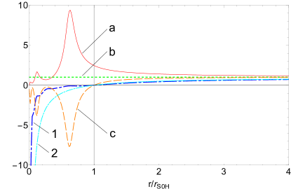
Figure 3: The solution for $c_{14}=2\times 10^{-7}$, $c_{2}=9\times 10^{-7}$, and $c_{3}=-c_{1}$. Here, $\tilde{A}$, $\tilde{B}$, $\tilde{J}$, $\tilde{F}$ and $\tilde{F}^{GR}$ are represented by the red line (labeled by a), green line (labeled by b), orange line (labeled by c), blue line (labeled by 1) and cyan line (labeled by 2) respectively.

As the first example, let us consider the case $c_{14}=2\times 10^{-7}$, $c_{2}=9\times 10^{-7}$, and $c_{3}=-c_{1}$, which satisfies the constraints (II). Fig. 3 shows the functions ${\tilde{F},\tilde{A},\tilde{B}}$, in which we also plot $\tilde{J}\equiv\tilde{F}\tilde{A}^{2}$ and the GR limit of $\tilde{F}$, denoted by $\tilde{F}^{GR}$ with $\tilde{F}^{GR}\equiv 1-r_{H}/r$.

In plotting Fig. 3, we chose $\epsilon=10^{-14}$. With the shooting method, $\tilde{A}_{H}$ is determined to be $\tilde{A}_{H}\simeq 2.4558992$ . In our calculations, we stop repeating the bisection search for $\tilde{A}_{H}$, when the value $\tilde{A}_{H}$ giving an asymptotically flat solution is determined to within $10^{-23}$. Technically, these accuracies could be further improved. However, for our current purposes, they are already sufficient.

As we have already mentioned, theoretically Eq. (3.76) will be automatically satisfied once Eqs. (3.74), (3.75) and (3.77) hold. However, due to numerical errors, in practice, it can never be zero numerically. Thus, to monitor our numerical errors, we always plot out the quantity $\tilde{\cal{C}}$ defined by Eq.(4.7), from which we can see clearly the numerical errors in our calculations. So, in the right-hand panels of Fig. 4, we plot out the curves of $\tilde{\cal{C}}$, denoted by $d$, in each case.

Clearly, outside the S0H, $\tilde{\cal{C}}\lesssim 10^{-17}$, while inside the S0H we have $\tilde{\cal{C}}\lesssim 10^{-10}$. Thus, the solutions inside the horizon are not as accurate as the ones given outside of the horizon. However, since in this paper we are mainly concerned with the spacetime outside of the S0H, we shall not consider further improvements of our numerical code inside the horizon. The other quantities, such as $c_{S}^{2}$ and $\tilde{r}_{g}$, are all given by the first row of Table 2.

Table 2: $c_{S}^{2}$, ${\tilde{A}}_{H}$ and $\tilde{r}_{g}/{r_{H}}$ calculated from different $\{c_{2},c_{14}\}$ with $c_{13}=0$ and a fixed ratio of $c_{2}/c_{14}$.

$c_{2}$	$c_{14}$	$c_{S}^{2}$	${\tilde{A}}_{H}$	$\tilde{r}_{g}/{r_{H}}$
$9\times 10^{-7}$	$2\times 10^{-7}$	$4.4999935$	2.4558992	1.1450729
$9\times 10^{-8}$	$2\times 10^{-8}$	$4.4999994$	2.4559003	1.1450730
$9\times 10^{-9}$	$2\times 10^{-9}$	$4.4999999$	2.4559004	1.1450730

Table 3: $c_{S}^{2}$, ${\tilde{A}}_{H}$ and $\tilde{r}_{g}/{r_{H}}$ calculated from different $\{c_{2},c_{14}\}$ with $c_{13}=0$ and changing $c_{2}/c_{14}$.

$c_{2}$	$c_{14}$	$c_{S}^{2}$	${\tilde{A}}_{H}$	$\tilde{r}_{g}/{r_{H}}$
$2.01\times 10^{-5}$	$2\times 10^{-5}$	$1.0049596$	1.4562430	1.0005850
$7\times 10^{-7}$	$5\times 10^{-7}$	$1.3999982$	1.6196457	1.0381205
$9\times 10^{-7}$	$2\times 10^{-8}$	$44.999939$	6.4676346	1.2629671
$9\times 10^{-5}$	$2\times 10^{-7}$	$449.93921$	19.053220	1.3091657

Following the same steps, we also consider other cases, and some of them are presented in Tables 2-3. In particular, in Table 2, we fix the ratio of $c_{2}/c_{14}$ to be 9/2. In addition, the values of $\{c_{2},c_{14}\}$ are chosen so that they satisfy the constraints of Eq.(II). In Table 3, the ratio $c_{2}/c_{14}$ is changing and the values of $\{c_{2},c_{14}\}$ are chosen so that they are spreading over the whole viable range of $c_{14}$, given by Eqs.(2.16)-(2.20).

From these tables we can see that quantities like $\tilde{A}_{H}$ and $\tilde{r}_{g}$ are sensitive only to the ratio of $c_{2}/c_{14}$, instead of their individual values. This is understandable, as for $c_{13}=0$ and $c_{14}\lesssim 2.5\times 10^{-5}$, Eq.(I) shows that $c_{S}\simeq c_{S}(c_{2}/c_{14})$. Therefore, the same ratio of $c_{2}/c_{14}$ implies the same velocity of the spin-0 graviton. Since S0H is defined by the speed of this massless particle, it is quite reasonable to expect that the related quantities are sensitive only to the value of $c_{S}$.

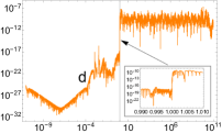
(a)	(b)
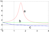
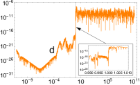
(c)	(d)
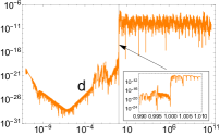
(e)	(f)

Figure 4: $\tilde{A}$, $\tilde{B}$ and $\tilde{F}$ for different combinations of $\{c_{2},c_{14}\}$ listed in Table 2 and their corresponding $\tilde{\cal{C}}$’s. Here the horizontal axis is $r_{H}/r$. $\tilde{A}$, $\tilde{B}$, $\tilde{F}$ and $\tilde{\cal{C}}$ are represented by the red solid line (labeled by a), green dotted line (labeled by b), blue dash-dotted line (labeled by c) and orange solid line (labeled by d) respectively. To be specific, (a) and (b) are for the case $\{9\times 10^{-7},2\times 10^{-7}\}$, (c) and (d) are for the case $\{9\times 10^{-8},2\times 10^{-8}\}$, (e) and (f) are for the case $\{9\times 10^{-9},2\times 10^{-9}\}$. Note that the small graphs inserted in (b), (d) and (f) show the amplifications of $\tilde{\cal{C}}$’s near $r=r_{H}$.

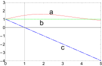
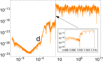
(a)	(b)
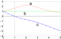
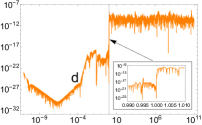
(c)	(d)
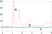
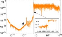
(e)	(f)
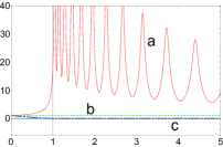
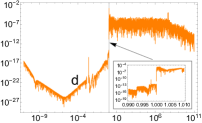
(g)	(h)

Figure 5: $\tilde{A}$, $\tilde{B}$ and $\tilde{F}$ for different combinations of $\{c_{2},c_{14}\}$ listed in Table 3 and their corresponding $\tilde{\cal{C}}$’s. Here the horizontal axis is $r_{H}/r$. $\tilde{A}$, $\tilde{B}$, $\tilde{F}$ and $\tilde{\cal{C}}$ are represented by the red solid line (labeled by a), green dotted line (labeled by b), blue dash-dotted line (labeled by c) and orange solid line (labeled by d) respectively. To be specific, (a) and (b) are for the case $\{2.01\times 10^{-5},2\times 10^{-5}\}$, (c) and (d) are for the case $\{7\times 10^{-7},5\times 10^{-7}\}$, (e) and (f) are for the case $\{9\times 10^{-7},2\times 10^{-8}\}$, (g) and (h) are for the case $\{9\times 10^{-5},2\times 10^{-7}\}$. Note that the small graphs inserted in (b), (d), (f) and (h) show the amplifications of $\tilde{\cal{C}}$ near $r=r_{H}$.

The resulting $\tilde{F}$, $\tilde{A}$, $\tilde{B}$ and $\tilde{\cal{C}}$ for the cases listed in Tables 2 and 3 are plotted in Figs. 4 and 5, respectively.

V Physical Solutions ($g_{\alpha\beta},\;u^{\mu}$)

The above steps reveal how we find the solutions of the effective metric $\tilde{g}_{\mu\nu}$ and aether field $\tilde{u}^{\mu}$. To find the corresponding physical quantities $g_{\mu\nu}$ and $u^{\mu}$, we shall follow two steps: (a) Reverse Eqs.(III.3) and (3.41) to find a set of the physical quantities $\{F(\xi),A(\xi),B(\xi)\}$ (Note that we have $\xi=\tilde{r}_{S0H}/r=r_{S0H}/r$). (b) Apply the rescaling $v\rightarrow C_{0}v$ to make the set of $\{F(\xi),A(\xi),B(\xi)\}$ take the standard form at spatial infinity $r=\infty$.

To these purposes, let us first note that, near the spatial infinity, Eqs.(III.4), (III.3) and (3.41) lead to

$$F(\xi) = \frac{C_{0}^{2}}{\sigma}\left(1+{F}_{1}\xi+\frac{1}{48}{c}_{14}{F}_{1}^{3}\xi^{3}\right){+{\cal O}\left(\xi^{4}\right)},$$

$$B(\xi) = \frac{C_{0}}{\sqrt{\sigma}}\left(1+\frac{1}{16}{c}_{14}{F}_{1}^{2}\xi^{2}-\frac{1}{12}{c}_{14}{F}_{1}^{3}\xi^{3}\right)$$

$$+{\cal O}\left(\xi^{4}\right),$$

$$A(\xi) = \frac{\sqrt{\sigma}}{C_{0}}\left[1-\frac{1}{2}{F}_{1}\xi+\frac{1}{2}A_{2}\xi^{2}\right.$$ (5.1)

$$\left.-\left(\frac{1}{2}{A}_{2}{F}_{1}-\frac{1}{16}{F}_{1}^{3}+\frac{1}{96}{c}_{14}{F}_{1}^{3}\right)\xi^{3}\right]$$

$$+{\cal O}\left(\xi^{4}\right),$$

where

$$F_{1} = \tilde{F}_{1},\quad c_{14}=\tilde{c}_{14},$$

$$A_{2} = \sqrt{\sigma}\tilde{A}_{2}-\frac{3}{4}(\sqrt{\sigma}-1)\tilde{F}_{1}^{2}.$$ (5.2)

The above expressions show clearly that the spacetimes described by $\left(g_{\mu\nu},u^{\mu}\right)$ are asymptotically flat, provided that the effective fields $\left(\tilde{g}_{\mu\nu},\tilde{u}^{\mu}\right)$ are. In particular, setting $C_{0}=\sqrt{\sigma}$, a condition that will be assumed in the rest of this section, the functions $F,\;A$ and $B$ will take their standard asymptotically-flat forms.

It is remarkable to note that the asymptotical behavior of the functions $F,\;A$ and $B$ depends only on $c_{14}$ up to the third-order of $\xi$, but $c_{2}$ will show up starting from the four-order of $\xi^{4}$.

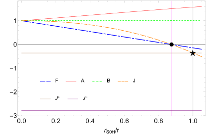
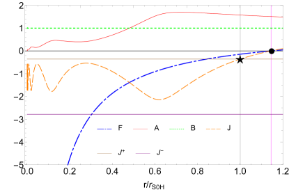
Figure 6: The evolutions of the physical quantities $F$, $A$, $B$ and $J$ for the case $c_{13}=0$, $c_{2}=9\times 10^{-7}$ and $c_{14}=2\times 10^{-7}$. Here, $A$, $B$, $J$ and $F$ are represented by the red solid line, green dotted line, orange dashed line, and blue dash-dotted line, respectively. The positions of $r=r_{MH}$ and $r=r_{S0H}$ are marked by a small full solid circle and a pentagram, respectively. Note that we have $r_{MH}>r_{S0H}$. The values $J^{+}$ and $J^{-}$ are given respectively by the brown and purple solid lines with $J^{+}>J^{-}$. The left panel shows the main behaviors of the functions outside the S0H in the range $r_{S0H}/r\in(0,1.105)$, while the right panel shows their main behaviors inside the S0H in the range $r/r_{S0H}\in(0,1.2)$.

V.1 Metric and Spin-0 Horizons

Again, we take the case of $c_{14}=2\times 10^{-7}$, $c_{2}=9\times 10^{-7}$, and $c_{3}=-c_{1}$ as the first example. The results for the normalized $F$, $A$, $B$ and $J$ in this case are plotted in Fig. 6. To see the whole picture of these functions on $r\in(0,\infty)$, they are plotted as functions of $r/r_{H}$ inside the horizon, while outside the horizon they are plotted as functions of $(r/r_{H})^{-1}$. This explains why in the left-hand panel of Fig. 6, the MH ($r=r_{MH}$) stays in the left-hand side of the S0H, while in the right-hand panel, they just reverse the order. In this figure, we didn’t plot the GR limits for $B$ and $F$ since they are almost overlapped with their counterparts. From the analysis of this case, we find the following:

(a) The values of $F$ and $B$ are almost equal to their GR limits all the time. This is true even when $r$ is approaching the center $r=0$, at which a spacetime curvature singularity is expected to be located.

(b) Inside the S0H, the oscillations of $A$ and $J$ become visible, which was also noted in Eling2006-2 . Such oscillations continue, and become more violent as the curvature singularity at the center is approaching.

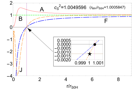
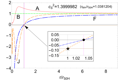
(a)	(b)
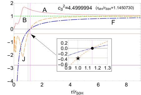
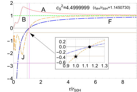
(c)	(d)
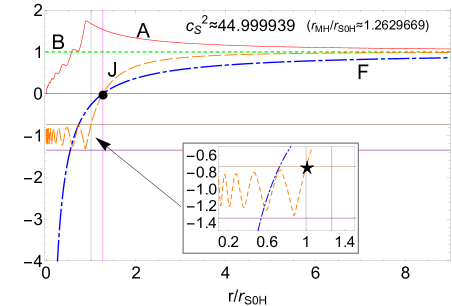
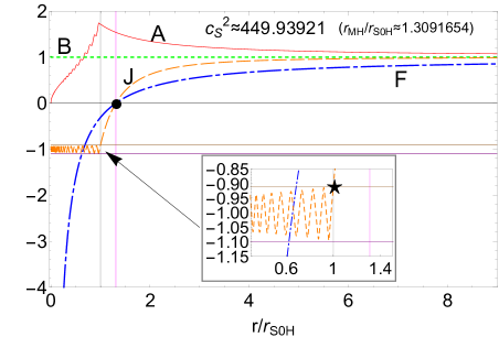
(e)	(f)

Figure 7: Solutions for different combinations of $\{c_{2},c_{14}\}$ listed in Tables 2-3. Here, $A$, $B$, $J$ and $F$ are represented by the red solid line, green dotted line, orange dashed line, and blue dash-dotted line, respectively. These figures are ordered according to the magnitude of $c_{S}^{2}$. In each of the figure, the values $J^{+}$ and $J^{-}$ are given respectively by the brown and purple solid lines with $J^{+}>J^{-}$, while the positions of $r=r_{MH}$ and $r=r_{S0H}$ are marked by a small full solid circle and a pentagram, respectively. Additionally, the value of $r_{MH}/r_{S0H}$ is also given in each case.

The functions of $\{F,A,B,J\}$ for the other cases listed in Tables 2-3 are plotted in Fig. 7. In this figure, the plots are ordered according to the magnitude of $c_{S}^{2}$. Besides, some amplified figures are inserted in (a)-(d) near the region around the point of $F=0$. Similarly, in (e)-(f), some amplified figures are inserted near the region around the point of $J=J^{+}$. The position of $r=r_{MH}$, at which we have $F(r_{MH})=0$, is marked by a full solid circle, while the position of $r=r_{S0H}$, at which we have $J(r_{S0H})=J^{+}$ [cf., Eq. (3.17)], is marked by a pentagram, and in all these cases we always have $r_{MH}>r_{S0H}$. The values of $J^{+}$ and $J^{-}$ are given by the brown and purple solid lines, respectively. Note we always have $J^{+}>J^{-}$ for $c_{S}>1$. By using these two lines, we can easily find that there is only one $r_{S0H}$ in each case, i.e., $r_{S0H}^{+}$ in Eq. (3.17).

From the studies of these representative cases, we find the following: (i) As we have already mentioned, in all these cases the functions $B$ and $F$ are very close to their GR limits. (ii) Changing $c_{S}^{2}$ won’t influence the maximum of $A$ much. In contrast, the maximum of $|J|$ inside the S0H is sensitive to $c_{S}^{2}$. (iii) The oscillation of $A(r)$ gets more violent as $c_{S}^{2}$ is increasing. (iv) The value of $|r_{MH}-r_{S0H}|$ is getting bigger as $c_{S}^{2}$ deviating from 1. (v) In all these cases, we have only one $r_{S0H}$, i.e., only one intersection between $J(r)$ and $J^{\pm}$, in each case. (vi) Just like what we saw in Tables 2-3, in the cases with the same $c_{S}$ (but different values of $c_{14}$ and $c_{2}$), the corresponding functions $\{F,A,B,J\}$ are quite similar.

From Tables 2-3 and Fig. 7, we would like also to note that the value of $r_{MH}$ is always close to the corresponding $\tilde{r}_{g}$. To understand this, let us consider Eq. (V), from which we find that

$$F(\xi) = 1+{F}_{1}\xi+\frac{1}{48}{c}_{14}{F}_{1}^{3}\xi^{3}+{\cal O}\left(\xi^{4},c_{14},c_{2}\right),~{}~{}~{}$$ (5.3)

after normalization. Recall $\xi\equiv r_{H}/r$ and $r_{H}\equiv r_{S0H}$. Then, from Eqs.(4.6), (III.4), (V) and (5.3), we also find that

$$\frac{\tilde{r}_{g}}{r_{S0H}}=-\tilde{F}_{1}=-F_{1}.$$ (5.4)

On the other hand, from Eq. (3.15), we have

$$\left.F(\xi)\right|_{r=r_{MH}} = 1+{F}_{1}\frac{r_{S0H}}{r_{MH}}+\frac{1}{48}{c}_{14}{F}_{1}^{3}\left(\frac{r_{S0H}}{r_{MH}}\right)^{3}$$ (5.5)

$$~{}~{}+{\cal O}\left(\xi^{4},c_{14},c_{2}\right)$$

$$= 0,$$

from which we obtain,

$$\frac{r_{MH}}{r_{S0H}} = -{F}_{1}-\frac{1}{48}{c}_{14}{F}_{1}^{3}\left(\frac{r_{S0H}}{r_{MH}}\right)^{2}+{\cal O}\left(\frac{r_{S0H}}{r_{MH}}\right)^{3}$$ (5.6)

$$= \frac{\tilde{r}_{g}}{r_{S0H}}+\frac{1}{48}{c}_{14}\left(\frac{\tilde{r}_{g}}{r_{S0H}}\right)^{3}\left(\frac{r_{S0H}}{r_{MH}}\right)^{2}$$

$$+{\cal O}\left(\xi^{3},c_{14},c_{2}\right),~{}~{}~{}~{}$$

where Eq.(5.4) was used. For the expansion of $F$ to be finite, we must assume

$${\cal O}\left(\xi^{3},c_{14},c_{2}\right)\lesssim{\cal{O}}\left[\frac{1}{48}{c}_{14}\left(\frac{\tilde{r}_{g}}{r_{S0H}}\right)^{3}\left(\frac{r_{S0H}}{r_{MH}}\right)^{2}\right].~{}~{}~{}~{}$$ (5.7)

At the same time, recall that we have $c_{14}\lesssim 2.5\times 10^{-5}$ and $r_{S0H}\leqslant r_{MH}$. Besides, we also have $\tilde{r}_{g}/r_{S0H}\simeq{\cal{O}}(1)$. Thus, from Eq. (5.6) we find

$$\left|\frac{r_{MH}}{r_{S0H}}-\frac{\tilde{r}_{g}}{r_{S0H}}\right|\lesssim{\cal{O}}(c_{14}).$$ (5.8)

This result reveals why the values of $r_{MH}/r_{S0H}$ and $\tilde{r}_{g}/r_{S0H}$ are very close to each other, although not necessarily the same exactly.

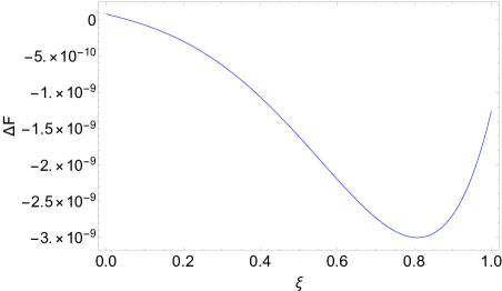
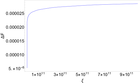
(a)	(b)
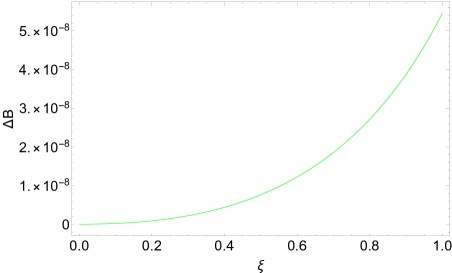
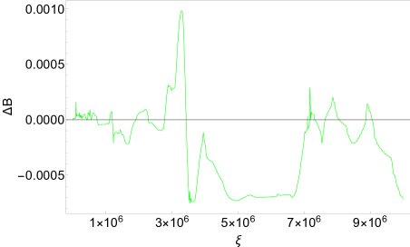
(c)	(d)

Figure 8: $\Delta F$ and $\Delta B$ for $c_{2}=9\times 10^{-7}$, $c_{14}=2\times 10^{-7}$ and $c_{13}=0$. The panels (a) and (c) show the region outside the S0H, while the panels (b) and (d) show the region inside the S0H.

Finally, let us take a closer look at the difference between GR and $\ae$-theory, although in the above we already mentioned that the results from these two theories are quite similar. To see these more clearly, we first note that the GR counterparts of $F$ and $B$ are given by

$$F^{GR}=1-\frac{r_{MH}}{r},\quad B^{GR}=1.$$ (5.9)

Thus, the relative differences can be defined as

$$\Delta F\equiv\frac{F-F^{GR}}{F^{GR}},\quad\Delta B\equiv\frac{B-B^{GR}}{B^{GR}}.$$ (5.10)

Again, considering the representative case $c_{2}=9\times 10^{-7}$, $c_{14}=2\times 10^{-7}$ and $c_{13}=0$, we plot out the differences $\Delta F$ and $\Delta B$ in Fig. 8, from which we find that in the range $\xi\in(10^{-12},1)$ we have ${\cal{O}}(\Delta F)\lesssim 10^{-9}$. On the other hand, in the range $\xi\in(1,10^{12})$, we have ${\cal{O}}(\Delta F)\lesssim 10^{-5}$. Similarly, in the range $\xi\in(10^{-12},1)$, we have ${\cal{O}}(\Delta B)\lesssim 10^{-8}$. In addition, in the range $\xi\in(1,10^{7})$ we have ${\cal{O}}(\Delta B)\lesssim 10^{-3}$. Thus, we confirm that $F$ and $B$ are indeed quite close to their GR limits.

Figure 9: Illustration of the bending of the $\phi$ = constant surfaces, and the existence of the UH in a spherically symmetric static spacetime, where $\phi$ denotes the globally timelike scalar field, and $t$ is the Painlevé-Gullstrand-like coordinates, which covers the whole spacetime LSW16 . Particles move always along the increasing direction of $\phi$. The Killing vector $\zeta^{\mu}=\delta^{\mu}_{v}$ always points upward at each point of the plane. The vertical dashed line is the location of the metric (Killing) horizon, $r=r_{MH}$. The UH, denoted by the vertical solid line, is located at $r=r_{UH}$, which is always inside the MH.

V.2 Universal Horizons

In theories with the broken LI, the dispersion relation of a massive particle contains generically high-order momentum terms Wang17 ,

$$E^{2}=m^{2}+c_{k}^{2}k^{2}\left(1+\sum^{2(z-1)}_{n=1}{a_{n}\left(\frac{k}{M_{*}}\right)^{n}}\right),$$ (5.11)

from which we can see that both of the group and phase velocities become unbounded as $k\rightarrow\infty$, where $E$ and $k$ are the energy and momentum of the particle considered, and $c_{k}$ and $a_{n}$’s are coefficients, depending on the species of the particle, while $M_{*}$ is the suppression energy scale of the higher-dimensional operators. Note that there must be no confusion between $c_{k}$ here and the four coupling constants $c_{i}$’s of the theory. As an immediate result, the causal structure of the spacetimes in such theories is quite different from that given in GR, where the light cone at a given point $p$ plays a fundamental role in determining the causal relationship of $p$ to other events GLLSW . In a UV complete theory, the above relationship is expected even in the gravitational sector. One of such examples is the healthy extension BPSa ; BPSb of Hořava gravity Horava ; Wang17 , a possible UV extension of the khronometric theory (the HO $\ae$-theory Jacobson10 ; Jacobson14 ).

However, once LI is broken, the causal structure will be dramatically changed. For example, in the Newtonian theory, time is absolute and the speeds of signals are not limited. Then, the causal structure of a given point $p$ is uniquely determined by the time difference, $\Delta{t}\equiv t_{p}-t_{q}$, between the two events. In particular, if $\Delta{t}>0$, the event $q$ is to the past of $p$; if $\Delta{t}<0$, it is to the future; and if $\Delta{t}=0$, the two events are simultaneous. In theories with breaking LI, a similar situation occurs.

To provide a proper description of BHs in such theories, UHs were proposed BS11 ; Enrico11 , which represent the absolute causal boundaries. Particles even with infinitely large speeds would just move on these boundaries and cannot escape to infinity. The main idea is as follows. In a given spacetime, a globally timelike scalar field $\phi$ may exist LACW . In the spherically symmetric case, this globally timelike scalar field can be identified to the HO aether field $u_{\mu}$ via the relation (2.46). Then, similar to the Newtonian theory, this field defines globally an absolute time, and all particles are assumed to move along the increasing direction of the timelike scalar field, so the causality is well defined. In such a spacetime, there may exist a surface at which the HO aether field $u_{\mu}$ is orthogonal to the timelike Killing vector, $\zeta\;(\equiv\partial_{v})$. Given that all particles move along the increasing direction of the HO aether field, it is clear that a particle must cross this surface and move inward, once it arrives at it, no matter how large its speed is. This is a one-way membrane, and particles even with infinitely large speeds cannot escape from it, once they are inside it [cf. Fig. 9]. So, it acts as an absolute horizon to all particles (with any speed), which is often called the UH BS11 ; Enrico11 ; Wang17 . At the horizon, as can be seen from Fig. 9, we have LGSW15 ,

$$\left.\zeta\cdot u\right|_{r=r_{UH}}=-\left.\frac{1}{2A}\left(1+J\right)\right|_{r=r_{UH}}=0,$$ (5.12)

where $J\equiv FA^{2}$. Therefore, the location of an UH is exactly the crossing point between the curve of $J(r)$ and the horizontal constant line $J=-1$, as one can see from Figs. 6 and 7. From these figures we can also see that they are always located inside S0Hs, as expected. In addition, the curve $J(r)$ is oscillating rapidly, and crosses the horizontal line $J=-1$ back and forth infinite times. Therefore, in each case we have infinite number of $r_{UH-i}\;(i=1,2,...)$. In this case, the UH is defined as the largest value of $r_{UH-i}\;(i=1,2,...)$. In Table 4, we show the locations of the first eight UHs for each case, listed in Tables 2 and 3. It is interesting to note that the formation of multi-roots of UHs was first noticed in Enrico11 , and later observed in gravitational collapse Bhattacharjee2018 .

V.3 Other Observational Quantities

Another observationally interesting quantity is the ISCO, which is the root of the equation,

$$2r{F^{\prime}(r)}^{2}-F\left[3F^{\prime}(r)+rF^{\prime\prime}(r)\right]=0.$$ (5.13)

Note that in GR we have $r_{ISCO}/r_{H}=3$ Paul2015 . Due to the tiny differences between the Schwarzschild solutions and the ones considered here, as shown in Fig. 8, it is expected that $r_{ISCO}$’s in these cases are also quite close to its GR limit. As a matter of fact, we find that this is indeed the case, and the differences in all the cases considered above appear only after six digits, that is, $\left|r_{ISCO}-r_{ISCO}^{GR}\right|\leq 10^{-6}$, as shown explicitly in Tables 5 and 6.

In Table 5, we also show several other physical quantities. These include the Lorentz gamma factor $\gamma_{ff}$, the gravitational radius $r_{g}$, the orbital frequency of the ISCO $\omega_{ISCO}$, the maximum redshift $z_{max}$ of a photon emitted by a source orbiting the ISCO (measured at the infinity), and the impact parameter $b_{ph}$ of the circular photon orbit (CPO), which are defined, respectively, by Enrico11 ,

$$\gamma_{ff} = \left.\left(A+\frac{1}{4A}\right)\right|_{r=r_{MH}},$$ (5.14)

$$r_{g} = \left.-r_{S0H}\frac{dF}{d\xi}\right|_{\xi\to 0},$$ (5.15)

$$\omega_{ISCO} = \left.\sqrt{\frac{dF/dr}{2r}}\right|_{r=r_{ISCO}},$$ (5.16)

$$z_{max} = \left.\frac{1+\omega_{ISCO}rF^{-1/2}}{\sqrt{F-\omega_{ISCO}^{2}r^{2}}}\right|_{r=r_{ISCO}}-1,~{}~{}~{}~{}~{}~{}~{}~{}$$ (5.17)

$$b_{ph} = \left.\frac{r}{\sqrt{F}}\right|_{r=r_{ph}},~{}~{}~{}~{}$$ (5.18)

where the radius $r_{ph}$ of the CPO is defined as

$$\left.\left(2F-r\frac{dF}{dr}\right)\right|_{r=r_{ph}}=0.$$ (5.19)

As pointed previously, these quantities are quite close to their relativistic limits, since they depend only on the spacetimes described by $F$ and $B$. As shown in Fig. 8, the differences of these spacetimes between $\ae$-theory and GR are very small. To see this more clearly, let us introduce the quantities,

$$\Delta r_{ISCO} \equiv \frac{r_{ISCO}}{r_{MH}}-\left(\frac{r_{ISCO}}{r_{MH}}\right)^{GR},$$

$$\Delta\omega_{ISCO} \equiv r_{g}\omega_{ISCO}-\left(r_{g}\omega_{ISCO}\right)^{GR},$$

$$\Delta z_{max} \equiv z_{max}-\left(z_{max}\right)^{GR},$$

$$\ \Delta b_{ph} \equiv \frac{b_{ph}}{r_{g}}-\left(\frac{b_{ph}}{r_{g}}\right)^{GR},$$ (5.20)

where the GR limits of $r_{ISCO}/r_{MH}$, $r_{g}\omega_{ISCO}$, $z_{max}$ and $b_{ph}/r_{g}$ are, respectively, $3,\;2\times 6^{-3/2}$, $3/\sqrt{2}-1$ and $3\sqrt{3}/2$. As can be seen from Table 6, all of these quantities are fairly close to their GR limits.

Therefore, we conclude that it is quite difficult to distinguish GR and $\ae$-theory through the considerations of the physical quantities $r_{ISCO}$, $\omega_{ISCO}$, $z_{max}$ or $b_{ph}$, as far as the cases considered in this paper are concerned. Thus, it would be very interesting to look for other choices of $\{c_{2},c_{13},c_{14}\}$ (if there exist), which could result in distinguishable values in these observational quantities.

Table 4: $r_{UH-i}$’s for different cases listed in Tables 2 and 3. Note that here we just show first eight UHs of Eq.(5.12) for each case.

$c_{S}^{2}$	$r_{MH}/r_{UH-1}$	$r_{MH}/r_{UH-2}$	$r_{MH}/r_{UH-3}$	$r_{MH}/r_{UH-4}$	$r_{MH}/r_{UH-5}$	$r_{MH}/r_{UH-6}$	$r_{MH}/r_{UH-7}$	$r_{MH}/r_{UH-8}$
1.0049596	1.40913534	9.12519836	68.6766490	524.111256	4006.80012	30638.7274	234291.582	1791613.54
1.3999982	1.39634652	6.27835216	33.1700700	178.825436	967.454326	5237.31538	28355.5481	153524.182
4.4999935	1.36429738	2.74101697	6.42094860	15.6447753	38.6164383	95.7784255	238.000717	591.850964
4.4999994	1.36429738	2.74101595	6.42094387	15.6447581	38.6163818	95.7782501	238.000194	591.849442
4.4999999	1.36429738	2.74101584	6.42094340	15.6447564	38.6163762	95.7782326	238.000141	591.849289
44.999939	1.33939835	1.56980254	1.91857535	2.41278107	3.08953425	4.00154026	5.22142096	6.84725395
449.93921	1.33429146	1.39226716	1.46010811	1.53855402	1.62835485	1.73026559	1.84507183	1.97362062

Table 5: The quantities $r_{S0H}$, $\gamma_{ff}$, $r_{ISCO}$, $\omega_{ISCO}$, $z_{max}$ and $b_{ph}$ for different cases listed in Tables 2 and 3 .

$c_{S}^{2}$	$r_{MH}/r_{S0H}$	$\gamma_{ff}$	$r_{ISCO}/r_{MH}$	$r_{g}\omega_{ISCO}$	$z_{max}$	$b_{ph}/r_{g}$
1.0049596	1.00058469	1.62614814	3.00000083	0.13608278	1.12132046	2.59807604
1.3999982	1.03812045	1.63971715	3.00000002	0.13608276	1.12132035	2.59807621
4.4999935	1.14507287	1.67376648	3.00000000	0.13608276	1.12132034	2.59807621
4.4999994	1.14507298	1.67376647	3.00000000	0.13608276	1.12132034	2.59807621
4.4999999	1.14507299	1.67376647	3.00000000	0.13608276	1.12132034	2.59807621
44.999939	1.26296693	1.69777578	3.00000000	0.13608276	1.12132034	2.59807621
449.93921	1.30916545	1.70149318	3.00000000	0.13608276	1.12132034	2.59807621

Table 6: $\Delta r_{ISCO}$, $\Delta\omega_{ISCO}$, $\Delta z_{max}$ and $\Delta b_{ph}$ for different cases listed in Tables 2 and 3 .

$c_{S}^{2}$	$\Delta r_{ISCO}$	$\Delta\omega_{ISCO}$	$\Delta z_{max}$	$\Delta b_{ph}$
1.0049596	$8.3\times 10^{-7}$	$1.3\times 10^{-8}$	$1.2\times 10^{-7}$	$-1.7\times 10^{-7}$
1.3999982	$1.8\times 10^{-8}$	$2.2\times 10^{-10}$	$2.0\times 10^{-9}$	$-3.2\times 10^{-9}$
4.4999935	$4.0\times 10^{-9}$	$1.5\times 10^{-12}$	$4.9\times 10^{-11}$	$-4.2\times 10^{-10}$
4.4999994	$4.0\times 10^{-10}$	$1.5\times 10^{-11}$	$-7.2\times 10^{-11}$	$-3.2\times 10^{-10}$
4.4999999	$4.0\times 10^{-11}$	$2.3\times 10^{-11}$	$-1.2\times 10^{-10}$	$-4.5\times 10^{-10}$
44.999939	$1.5\times 10^{-10}$	$9.6\times 10^{-11}$	$-5.6\times 10^{-10}$	$-1.9\times 10^{-9}$
449.93921	$1.1\times 10^{-9}$	$1.1\times 10^{-11}$	$-4.5\times 10^{-10}$	$-1.1\times 10^{-9}$

VI Conclusions

In this paper, we have systematically studied static spherically symmetric spacetimes in the framework of Einstein-aether theory, by paying particular attention to black holes that have regular S0Hs. In $\ae$-theory, a timelike vector - the aether, exists over the whole spacetime. As a result, in contrast to GR, now there are three gravitational modes, referred to as, respectively, the spin-0, spin-1 and spin-2 gravitons.

To avoid the vacuum gravi-Čerenkov radiation, all these modes must propagate with speeds greater than or at least equal to the speed of light EMS05 . However, in the spherically symmetric spacetimes, only the spin-0 mode is relevant in the gravitational sector Jacobson , and the boundaries of BHs are defined by this mode, which are the null surfaces with respect to the metric $g^{(S)}_{\mu\nu}$ defined in Eq.(1.3), the so-called S0Hs. Since now $c_{S}\geq c$, where $c_{S}$ is the speed of the spin-0 mode, the S0Hs are always inside or at most coincide with the metric (Killing) horizons. Then, in order to cover spacetimes both inside and outside the MHs, working in the Eddington-Finkelstein coordinates (3.1) is one of the natural choices.

In the process of gravitational radiations of compact objects, all of these three fundamental modes will be emitted, and the GW forms and energy loss rate should be different from that of GR. In particular, to the leading order, both monopole and dipole emissions will co-exist with the quadrupole emission Foster07 ; Yagi13 ; Yagi14 ; HYY15 ; Kai19 ; Zhao19 ; Zhang20 . Despite of all these, it is remarkable that the theory still remains as a viable theory, and satisfies all the constraints, both theoretical and observational OMW18 , including the recent detection of the GW, GW170817, observed by the LIGO/Virgo collaboration GW170817 , which imposed the severe constraint on the speed of the spin-2 gravitational mode, $-3\times 10^{-15}<c_{T}-1<7\times 10^{-16}$. Consequently, it is one of few theories that violate Lorentz symmetry and meantime is still consistent with all the observations carried out so far OMW18 ; Berti18a .

Spherically symmetric static BHs in $\ae$-theory have been extensively studied both analytically Eling2006-1 ; Oost2019 ; Per12 ; Dingq15 ; Ding16 ; Kai19b ; Ding19 ; Gao2013 ; Chan2020 ; Leon2019 ; Leon2020 and numerically Eling2006-2 ; Eling2007 ; Tamaki2008 ; BS11 ; Enrico11 ; Enrico2016 ; Zhu2019 , and various solutions have been obtained. Unfortunately, all these solutions have been ruled out by current observations OMW18 .

Therefore, as a first step, in this paper we have investigated spherically symmetric static BHs in $\ae$-theory that satisfy all the observational constraints found lately in OMW18 in detail, and presented various numerical new BH solutions. In particular, we have first shown explicitly that among the five non-trivial field equations, only three of them are independent. More important, the two second-order differential equations given by Eqs.(3.5) and (3.6) for the two functions $F(r)$ and $A(r)$ are independent of the function $B(r)$, where $F(r)$ and $B(r)$ are the metric coefficients of the Eddington-Finkelstein metric (3.1), and $A(r)$ describes the aether field, as shown by Eq.(3.2). Thus, one can first solve Eqs.(3.5) and (3.6) to find $F(r)$ and $A(r)$, and then from the third independent equation to find $B(r)$. Another remarkable feature is that the function $B(r)$ can be obtained from the constraint (3.10), and is given simply by the algebraic expression of $F,\;A$ and their derivatives, as shown explicitly by Eq.(3.11). This not only saves the computational labor, but also makes the calculations more accurate, as pointed out explicitly in Enrico11 , solving the first-order differential equation (3.7) for $B(r)$ can “potentially be affected by numerical inaccuracies when evaluated very close to the horizon”.

Then, now solving the (vacuum) field equations of spherically symmetric static spacetimes in $\ae$-theory simply reduces to solve the two second-order differential equations (3.5) and (3.6). This will considerably simplify the mathematical computations, which is very important, especially considering the fact that the field equations involved are extremely complicated, as one can see from Eqs.(3.5)-(3.10) and (Appendix A: The coefficients of $f_{n},a_{n},b_{n}$ and $n_{n}$) - (Appendix A: The coefficients of $f_{n},a_{n},b_{n}$ and $n_{n}$). Then, in the case $c_{13}=c_{14}=0$ we have been able to solve these equations explicitly, and obtained a three-parameter family of exact solutions, which in general depends on the coupling constant $c_{2}$. However, requiring that the solutions be asymptotically flat, we have found that the solutions become independent of $c_{2}$, and the corresponding metric reduces precisely to the Schwarzschild BH solution with a non-trivially coupling aether field given by Eq.(3.34), which is always timelike even in the region inside the BH.

To simplify the problem further, we have also taken the advantage of the field redefinitions that are allowed by the internal symmetry of $\ae$-theory, first discovered by Foster in Foster05 , and later were used frequently, including the works of Eling2006-2 ; Tamaki2008 ; Enrico11 . The advantage of the field redefinitions is that it allows us to choose the free parameter $\sigma$ involved in the field redefinitions, so that the S0H of the redefined metric $\tilde{g}_{\mu\nu}$ will coincide with its MH. This will reduce the four-dimensional space of the initial conditions, spanned by $\tilde{F}_{H},\;\tilde{F}^{\prime}_{H},\;\tilde{A}_{H},\;\tilde{A}^{\prime}_{H}$, to one-dimension, spanned only by $\tilde{A}_{H}$, if the initial conditions are imposed on the S0H. In Sec. III.D. we have shown step by step how one can do it. In addition, in this same subsection we have also shown that the field equations are invariant under the rescaling $r\rightarrow Cr$. In fact, introducing the dimensionless coordinate $\xi\equiv r_{S0H}/r$, the relevant four field equations take the scaling-invariant forms of Eqs.(3.74) - (3.77), which are all independent of $r_{S0H}$. Thus, when integrating these equations, without loss of generality, one can assign any value to $r_{S0H}$.

We would like also to note that in Section III.C we worked out the relations in detail among the fields ($g_{\mu\nu},u^{\mu},c_{i})$, ($\hat{g}_{\mu\nu},\hat{u}^{\mu},\hat{c}_{i})$ and ($\tilde{g}_{\mu\nu},\tilde{u}^{\mu},\tilde{c}_{i})$, and clarified several subtle points. In particular, the redefined metric $\hat{g}_{\mu\nu}$ through Eqs.(II.1) and (II.1) does not take the standard form in the Eddington-Finkelstein coordinates, as shown explicitly by Eq.(3.35). Instead, only after a proper coordinate transformation given by Eqs.(3.36) and (3.37), the resulting metric $\tilde{g}_{\mu\nu}$ takes the standard form, as given by Eq.(3.38). Then, the field equations for ($\tilde{g}_{\mu\nu},\tilde{u}^{\mu},\tilde{c}_{i})$ take the same forms as the ones for ($g_{\mu\nu},u^{\mu},c_{i})$. Therefore, when we solved the field equations in terms of the redefined fields, they are the ones of ($\tilde{g}_{\mu\nu},\;\tilde{u}^{\mu}$), not the ones for ($\hat{g}_{\mu\nu},\;\hat{u}^{\mu}$).

After clarifying all these subtle points, in Sec. IV, we have worked out the detail on how to carry out explicitly our numerical analysis. In particular, to monitor the numerical errors of our code, we have introduced the quantity $\tilde{\cal{C}}$ through Eq.(4.7), which is essentially Eq.(3.65). Theoretically, it vanishes identically. But, due to numerical errors, it is expected that $\tilde{\cal{C}}$ has non-zero values, and the amplitude of it will provide a good indication on the numerical errors that our numerical code could produce.

To show further the accuracy of our numerical code, we have first reproduced the BH solutions obtained in Eling2006-2 ; Enrico11 , but with an accuracy that are at least two orders higher [cf. Table 1]. It should be noted that all these BH solutions have been ruled out by the current observations OMW18 . So, after checking our numerical code, in Sec. IV.B, we considered various new BH solutions that satisfy all the observational constraints OMW18 , and presented them in Tables 2 and 3, as well as in Figs. 3-5.

Then, in Sec. V, we have presented the physical metric $g_{\mu\nu}$ and $\ae$-field $u^{\mu}$ for these viable new BH solutions obtained in Section IV. Before presenting the results, we have first shown that the physical fields, ${g}_{\mu\nu}$ and ${u}^{\mu}$, are also asymptotically flat, provided that the effective fields $\tilde{g}_{\mu\nu}$ and $\tilde{u}^{\mu}$ are [cf. Eqs.(V) and (V)]. Then, the physical BH solutions were plotted out in Figs. 6 and 7. Among several interesting features, we would like to point out the different locations of the metric and spin-0 horizons for the physical metric ${g}_{\mu\nu}$, denoted by full solid circles and pentagrams, respectively.

Another interesting point is that all these physical BH solutions are quite similar to the Schwarzschild one. In Fig. 8 we have shown the differences for the case $c_{2}=9\times 10^{-7}$, $c_{14}=2\times 10^{-7}$ and $c_{13}=0$, but similar results also hold for the other cases, listed in Tables 2 and 3.

In this section, we have also identified the locations of the UHs of these solutions and several other observationally interesting quantities, which include the ISCO $r_{ISCO}$, the Lorentz gamma factor $\gamma_{ff}$, the gravitational radius $r_{g}$, the orbital frequency $\omega_{ISCO}$ of the ISCO, the maximum redshift $z_{max}$ of a photon emitted by a source orbiting the ISCO (measured at the infinity), the radii $r_{ph}$ of the CPO, and the impact parameter $b_{ph}$ of the CPO. All of them are given in Table 4-5. In Table 6 we also calculated the differences of these quantities obtained in $\ae$-theory and GR. Looking at these results, we conclude that it’s very hard to distinguish GR and $\ae$-theory through these quantities, as far as the cases considered in this paper are concerned. We would also like to note that for each BH solution, there are infinite number of UHs, $r=r_{UH-i},\;(i=1,2,3,...)$, which was also observed in Enrico11 . In Table 4 we have listed the first eight of them, and the largest one is usually defined as the UH of the BH. In contrast, there are only one S0H and one MH for each solution. These features are also found in the gravitational collapse of a massless scalar field in $\ae$-theory Bhattacharjee2018 .

An immediate implication of the above results is that the QNMs of these BHs for a test field, scalar, vector or tensor KZ07a , will be quite similar to these given in GR. Our preliminary results on such studies indicate that this is indeed the case. However, we expect that there should be significant differences from GR, when we consider the metric perturbations of these BH solutions - the gravitational spectra of perturbations KZ07b , as now the BH boundaries are the locations of the S0Hs, not the locations of the MHs. This should be specially true for the cases with large speeds $c_{S}$ of the spin-0 modes, as in these cases the S0Hs are significantly different from the MHs, and located deeply inside them. Thus, imposing the non-out-going radiation on the S0Hs will be quite different from imposing the non-out-going radiation on the corresponding MHs. We wish to report our results along this direction soon in another occasion.

Appendix A: The coefficients of $f_{n},a_{n},b_{n}$ and $n_{n}$

In this appendix, we shall provide the explicit expressions of the coefficients of $f_{n},a_{n},b_{n}$ and $n_{n}$, encountered in the Einstein-aether field equations in the spherically symmetric spacetimes, for which the metric is written in the Eddington-Finkelstein coordinates (3.1), with the aether field taking the form of Eq.(3.2). In particular, the coefficients of $f_{n},a_{n}$ and $b_{n}$ appearing in Eqs.(3.5) - (3.7) are given by,

$$f_{0} = -4\left(c_{2}+c_{13}\right)\left(c_{2}+c_{13}-\left(c_{2}+1\right)c_{14}\right)rA(r)A^{\prime}(r)$$

$$-\left(c_{14}c_{2}^{2}-c_{2}^{2}+c_{13}^{2}+\left(c_{2}+1\right)c_{14}^{2}-\left(c_{2}+2\right)c_{13}c_{14}\right)r^{2}A^{\prime}(r)^{2}$$

$$-4\left(\left(c_{14}+1\right)c_{13}^{2}+2\left(c_{2}+1\right)c_{13}+\left(c_{2}-2\right)c_{14}c_{13}+c_{2}\left(c_{2}+2\right)-2\left(c_{2}^{2}+3c_{2}+1\right)c_{14}\right)rA(r)^{4}F^{\prime}(r)$$

$$+2\left(c_{2}^{2}+\left(2-3c_{2}\right)c_{14}c_{2}-9c_{13}c_{14}c_{2}+\left(c_{2}+1\right)c_{14}^{2}-c_{13}^{2}\left(4c_{14}+1\right)\right)r^{2}A(r)^{3}A^{\prime}(r)F^{\prime}(r)$$

$$-\left(5c_{14}c_{2}^{2}-c_{2}^{2}+\left(c_{2}+1\right)c_{14}^{2}+\left(7c_{2}-2\right)c_{13}c_{14}+c_{13}^{2}\left(4c_{14}+1\right)\right)r^{2}A(r)^{6}F^{\prime}(r)^{2}$$

$$-2\left(c_{2}+c_{13}\right)c_{14}\left(-c_{2}+c_{13}+c_{14}-4\right)r^{3}A(r)^{5}A^{\prime}(r)F^{\prime}(r)^{2}+\left(c_{2}+c_{13}\right)c_{14}\left(c_{2}-c_{13}+c_{14}\right)r^{3}A(r)^{8}F^{\prime}(r)^{3}$$

$$-\left(c_{2}+c_{13}\right)A(r)^{2}\left(-c_{14}\left(c_{2}-c_{13}+c_{14}\right)r^{3}A^{\prime}(r)^{2}F^{\prime}(r)+4c_{2}\left(c_{14}-1\right)+2c_{13}c_{14}\right),$$

$$f_{1} = -8\left(c_{2}+c_{13}\right)\left(c_{14}c_{2}+c_{2}+c_{13}+c_{14}\right)rA(r)^{3}A^{\prime}(r)$$

$$+4\left(c_{2}^{2}-3c_{13}c_{14}c_{2}+2c_{14}c_{2}+\left(c_{2}+1\right)c_{14}^{2}-c_{13}^{2}\left(c_{14}+1\right)\right)r^{2}A(r)^{2}A^{\prime}(r)^{2}$$

$$-4\left(\left(1-2c_{14}\right)c_{13}^{2}+\left(-c_{14}c_{2}+2c_{2}+c_{14}+4\right)c_{13}+c_{2}\left(c_{2}+4\right)+\left(5c_{2}^{2}+9c_{2}+4\right)c_{14}\right)rA(r)^{6}F^{\prime}(r)$$

$$+2\left(c_{14}c_{2}^{2}+3c_{2}^{2}-3\left(c_{2}+1\right)c_{14}^{2}+\left(11c_{2}+6\right)c_{13}c_{14}+c_{13}^{2}\left(4c_{14}-3\right)\right)r^{2}A(r)^{5}A^{\prime}(r)F^{\prime}(r)$$

$$+2\left(c_{2}^{2}+\left(3c_{2}+2\right)c_{14}c_{2}+3c_{13}c_{14}c_{2}+\left(c_{2}+1\right)c_{14}^{2}+c_{13}^{2}\left(2c_{14}-1\right)\right)r^{2}A(r)^{8}F^{\prime}(r)^{2}$$

$$+2\left(c_{2}+c_{13}\right)c_{14}\left(c_{2}-c_{13}+c_{14}\right)r^{3}A(r)^{7}A^{\prime}(r)F^{\prime}(r)^{2}$$

$$-2\left(c_{2}+c_{13}\right)c_{14}A(r)^{4}\left(\left(-c_{2}+c_{13}+c_{14}-4\right)r^{3}A^{\prime}(r)^{2}F^{\prime}(r)-4\left(2c_{2}+c_{13}+1\right)\right),$$

$$f_{2} = 2\left(c_{14}c_{2}^{2}+3c_{2}^{2}-3\left(c_{2}+1\right)c_{14}^{2}+\left(11c_{2}+6\right)c_{13}c_{14}+c_{13}^{2}\left(4c_{14}-3\right)\right)r^{2}A(r)^{4}A^{\prime}(r)^{2}$$

$$+4\left(-\left(c_{14}-1\right)c_{13}^{2}+2\left(c_{2}-1\right)c_{13}+\left(c_{2}+4\right)c_{14}c_{13}+\left(c_{2}-2\right)c_{2}+\left(4c_{2}^{2}+8c_{2}+2\right)c_{14}\right)rA(r)^{8}F^{\prime}(r)$$

$$+6\left(\left(c_{14}+1\right)c_{2}^{2}+c_{14}\left(-c_{13}+c_{14}+2\right)c_{2}-c_{13}^{2}+c_{14}^{2}\right)r^{2}A(r)^{7}A^{\prime}(r)F^{\prime}(r)$$

$$+\left(-\left(c_{14}-1\right)c_{2}^{2}+\left(c_{13}-c_{14}\right)c_{14}c_{2}-\left(c_{13}-c_{14}\right){}^{2}\right)r^{2}A(r)^{10}F^{\prime}(r)^{2}$$

$$+\left(-c_{2}-c_{13}\right)A(r)^{6}\left(-c_{14}\left(c_{2}-c_{13}+c_{14}\right)r^{3}A^{\prime}(r)^{2}F^{\prime}(r)+8c_{2}+4\left(6c_{2}+3c_{13}+4\right)c_{14}\right),$$

$$f_{3} = 8\left(c_{2}+c_{13}\right)\left(c_{14}c_{2}+c_{2}+c_{13}+c_{14}\right)rA(r)^{7}A^{\prime}(r)+8\left(2c_{2}^{2}+3c_{13}c_{2}+c_{2}+c_{13}^{2}+c_{13}\right)c_{14}A(r)^{8}$$

$$+4\left(c_{2}^{2}-3c_{13}c_{14}c_{2}+2c_{14}c_{2}+\left(c_{2}+1\right)c_{14}^{2}-c_{13}^{2}\left(c_{14}+1\right)\right)r^{2}A(r)^{6}A^{\prime}(r)^{2}$$

$$+4\left(c_{2}+c_{13}\right)\left(c_{2}+c_{13}-\left(c_{2}+1\right)c_{14}\right)rA(r)^{10}F^{\prime}(r)$$

$$+2\left(c_{2}-c_{13}+c_{14}\right)\left(c_{2}+c_{13}-\left(c_{2}+1\right)c_{14}\right)r^{2}A(r)^{9}A^{\prime}(r)F^{\prime}(r),$$

$$f_{4} = 4\left(c_{2}+c_{13}\right)\left(c_{2}+c_{13}-\left(c_{2}+1\right)c_{14}\right)rA(r)^{9}A^{\prime}(r)-2\left(c_{2}+c_{13}\right)\left(2c_{2}\left(c_{14}-1\right)+c_{13}c_{14}\right)A(r)^{10}$$ (A.1)

$$+\left(-c_{14}c_{2}^{2}+c_{2}^{2}-c_{13}^{2}-\left(c_{2}+1\right)c_{14}^{2}+\left(c_{2}+2\right)c_{13}c_{14}\right)r^{2}A(r)^{8}A^{\prime}(r)^{2},$$

$$a_{0} = 4\left(-\left(c_{14}-1\right)c_{13}^{2}+\left(-c_{14}c_{2}+2c_{2}+2c_{14}-2\right)c_{13}+\left(c_{2}-2\right)c_{2}+2\left(c_{2}^{2}+3c_{2}+1\right)c_{14}\right)rA(r)^{2}A^{\prime}(r)$$

$$+\left(c_{13}^{2}+\left(5c_{2}c_{14}+8\right)c_{13}-\left(c_{2}+1\right)c_{14}^{2}-\left(c_{2}-8\right)c_{2}-\left(5c_{2}^{2}+18c_{2}+8\right)c_{14}\right)r^{2}A(r)A^{\prime}(r)^{2}$$

$$+\left(c_{2}+c_{13}\right)c_{14}\left(c_{2}-c_{13}+c_{14}\right)r^{3}A^{\prime}(r)^{3}+4\left(c_{2}+c_{13}\right)\left(c_{14}c_{2}+c_{2}+c_{13}+c_{14}\right)rA(r)^{5}F^{\prime}(r)$$

$$-2\left(\left(2c_{14}-1\right)c_{13}^{2}+\left(\left(3c_{2}-2\right)c_{14}+4\right)c_{13}-\left(c_{2}+1\right)c_{14}^{2}+c_{2}\left(c_{2}+4\right)+\left(3c_{2}^{2}+4c_{2}+4\right)c_{14}\right)r^{2}A(r)^{4}A^{\prime}(r)F^{\prime}(r)$$

$$+\left(-c_{2}^{2}-\left(c_{2}+2\right)c_{14}c_{2}+c_{13}c_{14}c_{2}+c_{13}^{2}-\left(c_{2}+1\right)c_{14}^{2}\right)r^{2}A(r)^{7}F^{\prime}(r)^{2}$$

$$+\left(c_{2}+c_{13}\right)c_{14}\left(c_{2}-c_{13}+c_{14}\right)r^{3}A(r)^{6}A^{\prime}(r)F^{\prime}(r)^{2}$$

$$-2\left(c_{2}+c_{13}\right)A(r)^{3}\left(c_{14}\left(-c_{2}+c_{13}+c_{14}-4\right)r^{3}A^{\prime}(r)^{2}F^{\prime}(r)+2c_{2}+2c_{2}c_{14}+c_{13}c_{14}+4\right),$$

$$a_{1} = 4\left(\left(2c_{14}+1\right)c_{13}^{2}+\left(3c_{14}c_{2}+2c_{2}+c_{14}-4\right)c_{13}+\left(c_{2}-4\right)c_{2}-\left(3c_{2}^{2}+7c_{2}+4\right)c_{14}\right)rA(r)^{4}A^{\prime}(r)$$

$$+\left(-\left(8c_{14}-3\right)c_{13}^{2}-\left(\left(23c_{2}+14\right)c_{14}-8\right)c_{13}+3\left(c_{2}+1\right)c_{14}^{2}-c_{2}\left(3c_{2}-8\right)-\left(c_{2}^{2}-8c_{2}-8\right)c_{14}\right)r^{2}A(r)^{3}A^{\prime}(r)^{2}$$

$$-2\left(c_{2}+c_{13}\right)c_{14}\left(-c_{2}+c_{13}+c_{14}-4\right)r^{3}A(r)^{2}A^{\prime}(r)^{3}-8\left(c_{2}+1\right)\left(c_{2}+c_{13}\right)c_{14}rA(r)^{7}F^{\prime}(r)$$

$$+4\left(\left(c_{14}+1\right)c_{13}^{2}+2\left(c_{2}c_{14}-1\right)c_{13}-\left(c_{2}+1\right)c_{14}^{2}-c_{2}\left(c_{2}+2\right)+\left(c_{2}^{2}+2c_{2}+2\right)c_{14}\right)r^{2}A(r)^{6}A^{\prime}(r)F^{\prime}(r)$$

$$+\left(c_{14}c_{2}^{2}-c_{2}^{2}+c_{13}^{2}+\left(c_{2}+1\right)c_{14}^{2}-\left(c_{2}+2\right)c_{13}c_{14}\right)r^{2}A(r)^{9}F^{\prime}(r)^{2}$$

$$-2\left(c_{2}+c_{13}\right)A(r)^{5}\left(-c_{14}\left(c_{2}-c_{13}+c_{14}\right)r^{3}A^{\prime}(r)^{2}F^{\prime}(r)-2c_{2}-\left(6c_{2}+3c_{13}+4\right)c_{14}\right),$$

$$a_{2} = -2\left(c_{2}+c_{13}\right)\left(\left(6c_{2}+3c_{13}+4\right)c_{14}-2\left(c_{2}+2\right)\right)A(r)^{7}$$

$$-4\left(\left(c_{14}+1\right)c_{13}^{2}+\left(c_{2}\left(3c_{14}+2\right)+2\right)c_{13}+c_{2}\left(c_{2}+2\right)-2\left(2c_{2}+1\right)c_{14}\right)rA(r)^{6}A^{\prime}(r)$$

$$+\left(-3c_{2}^{2}+\left(5c_{2}-6\right)c_{14}c_{2}+19c_{13}c_{14}c_{2}-3\left(c_{2}+1\right)c_{14}^{2}+c_{13}^{2}\left(8c_{14}+3\right)\right)r^{2}A(r)^{5}A^{\prime}(r)^{2}$$

$$+\left(c_{2}+c_{13}\right)c_{14}\left(c_{2}-c_{13}+c_{14}\right)r^{3}A(r)^{4}A^{\prime}(r)^{3}-4\left(c_{2}+c_{13}\right)\left(c_{2}+c_{13}-\left(c_{2}+1\right)c_{14}\right)rA(r)^{9}F^{\prime}(r)$$

$$-2\left(c_{2}-c_{13}+c_{14}\right)\left(c_{2}+c_{13}-\left(c_{2}+1\right)c_{14}\right)r^{2}A(r)^{8}A^{\prime}(r)F^{\prime}(r),$$

$$a_{3} = 2\left(c_{2}+c_{13}\right)\left(2c_{2}\left(c_{14}-1\right)+c_{13}c_{14}\right)A(r)^{9}-4\left(c_{2}+c_{13}\right)\left(c_{2}+c_{13}-\left(c_{2}+1\right)c_{14}\right)rA(r)^{8}A^{\prime}(r)$$

$$+\left(c_{14}c_{2}^{2}-c_{2}^{2}+c_{13}^{2}+\left(c_{2}+1\right)c_{14}^{2}-\left(c_{2}+2\right)c_{13}c_{14}\right)r^{2}A(r)^{7}A^{\prime}(r)^{2},$$

and

$$b_{0} = 4\left(c_{2}+1\right)\left(c_{2}+c_{13}\right)c_{14}A(r)^{2}-4\left(c_{2}+c_{13}\right){}^{2}c_{14}rA(r)A^{\prime}(r)$$

$$+\left(c_{2}+c_{13}\right)c_{14}\left(c_{2}-c_{13}+c_{14}\right)r^{2}A^{\prime}(r)^{2}-4\left(c_{2}+c_{13}\right){}^{2}c_{14}rA(r)^{4}F^{\prime}(r)$$

$$-2\left(c_{2}+c_{13}\right)c_{14}\left(-c_{2}+c_{13}+c_{14}-4\right)r^{2}A(r)^{3}A^{\prime}(r)F^{\prime}(r)$$

$$+\left(c_{2}+c_{13}\right)c_{14}\left(c_{2}-c_{13}+c_{14}\right)r^{2}A(r)^{6}F^{\prime}(r)^{2},$$

$$b_{1} = -2\left(c_{2}+c_{13}\right)c_{14}\left(-c_{2}+c_{13}+c_{14}-4\right)r^{2}A(r)^{2}A^{\prime}(r)^{2}-8\left(c_{2}+1\right)\left(c_{2}+c_{13}\right)c_{14}A(r)^{4}$$

$$+2\left(c_{2}+c_{13}\right)c_{14}\left(c_{2}-c_{13}+c_{14}\right)r^{2}A(r)^{5}A^{\prime}(r)F^{\prime}(r)+4\left(c_{2}+c_{13}\right){}^{2}c_{14}rA(r)^{6}F^{\prime}(r),$$

$$b_{2} = 4\left(c_{2}+c_{13}\right){}^{2}c_{14}rA(r)^{5}A^{\prime}(r)+4\left(c_{2}+1\right)\left(c_{2}+c_{13}\right)c_{14}A(r)^{6}$$ (A.3)

$$+\left(c_{2}+c_{13}\right)c_{14}\left(c_{2}-c_{13}+c_{14}\right)r^{2}A(r)^{4}A^{\prime}(r)^{2}.$$

On the other hand, the coefficients $n_{n}$’s appearing in Eq.(3.10) are given by

$$n_{0} = \frac{c_{2}A^{\prime}(r)}{2rA(r)^{3}B(r)^{3}}-\frac{c_{2}}{2r^{2}A(r)^{2}B(r)^{3}}-\frac{c_{13}}{4r^{2}A(r)^{2}B(r)^{3}}-\frac{1}{r^{2}B(r)}$$

$$-\frac{\left(c_{2}+c_{13}+c_{14}\right)A^{\prime}(r)F^{\prime}(r)}{4A(r)B(r)^{3}}-\frac{\left(c_{2}+c_{13}-c_{14}\right)A^{\prime}(r)^{2}}{8A(r)^{4}B(r)^{3}}+\frac{\left(c_{2}+2\right)F^{\prime}(r)}{2rB(r)^{3}}$$

$$-\frac{\left(c_{2}+c_{13}-c_{14}\right)A(r)^{2}F^{\prime}(r)^{2}}{8B(r)^{3}},$$

$$n_{1} = \frac{\left(-c_{2}-c_{13}-c_{14}\right)A^{\prime}(r)^{2}}{4A(r)^{2}B(r)^{3}}-\frac{c_{2}A(r)^{2}F^{\prime}(r)}{2rB(r)^{3}}+\frac{2c_{2}+c_{13}+2}{2r^{2}B(r)^{3}}$$

$$+\frac{\left(-c_{2}-c_{13}+c_{14}\right)A(r)A^{\prime}(r)F^{\prime}(r)}{4B(r)^{3}},$$

$$n_{2} = -\frac{c_{2}A(r)A^{\prime}(r)}{2rB(r)^{3}}+\frac{\left(-c_{2}-c_{13}+c_{14}\right)A^{\prime}(r)^{2}}{8B(r)^{3}}+\frac{\left(-2c_{2}-c_{13}\right)A(r)^{2}}{4r^{2}B(r)^{3}}.$$ (A.4)

When $c_{S}=1$, i.e. $c_{2}=\left(-2c_{13}+2c_{14}-c_{13}^{2}c_{14}\right)/\left(2-4c_{14}+3c_{13}c_{14}\right)$, the coefficients $f_{0},a_{0},b_{0}$ and $n_{0}$ reduce to

$$f_{0} = \left[rA(r)^{2}F^{\prime}(r)+\frac{c_{14}c_{13}+2c_{13}-2c_{14}}{2\left(c_{13}-1\right)c_{14}}\right]b_{0},$$

$$a_{0} = \frac{2\left(c_{13}-1\right)c_{14}rA^{\prime}(r)+\left(c_{13}-2\right)\left(c_{14}-2\right)A(r)}{c_{13}\left(c_{14}\left(2rA(r)^{2}F^{\prime}(r)+1\right)+2\right)-2c_{14}\left(rA(r)^{2}F^{\prime}(r)+1\right)}f_{0},$$

$$b_{0} = \frac{1}{\left(\left(3c_{13}-4\right)c_{14}+2\right){}^{2}}\left\{-2\left(c_{13}-1\right){}^{2}c_{14}^{2}\left(4c_{14}c_{13}^{2}+\left(-3c_{14}^{2}-4c_{14}+4\right)c_{13}+4\left(c_{14}-1\right)c_{14}\right)r^{2}A^{\prime}(r)^{2}\right.$$ (A.5)

$$\left.-4\left(c_{13}-1\right){}^{2}c_{14}^{2}rA(r)A^{\prime}(r)\left[\left(4c_{14}c_{13}^{2}+\left(3c_{14}^{2}-16c_{14}+4\right)c_{13}-4\left(c_{14}^{2}-4c_{14}+2\right)\right)rA(r)^{2}F^{\prime}(r)\right.\right.$$

$$\left.\left.+4\left(c_{13}-1\right){}^{2}c_{14}\right]-2\left(c_{13}-1\right){}^{2}c_{14}^{2}A(r)^{2}\left[\left(4c_{14}c_{13}^{2}+\left(-3c_{14}^{2}-4c_{14}+4\right)c_{13}\right.\right.\right.$$

$$\left.\left.\left.+4\left(c_{14}-1\right)c_{14}\right)r^{2}A(r)^{4}F^{\prime}(r)^{2}+8\left(c_{13}-1\right){}^{2}c_{14}rA(r)^{2}F^{\prime}(r)+4\left(c_{13}-1\right)\left(\left(c_{13}-2\right)c_{14}+2\right)\right]\right\},$$

and

$$n_{0} = \frac{c_{14}\left(-2c_{13}^{2}+\left(3c_{14}+4\right)c_{13}-4c_{14}\right)A(r)^{2}F^{\prime}(r)^{2}}{8\left(\left(3c_{13}-4\right)c_{14}+2\right)B(r)^{3}}$$ (A.6)

$$+F^{\prime}(r)\left[\left(c_{14}\left(-2c_{13}^{2}-3c_{14}c_{13}+4c_{13}+4c_{14}-4\right)rA^{\prime}(r)-2\left(c_{14}c_{13}^{2}+\left(2-6c_{14}\right)c_{13}+6c_{14}-4\right)A(r)\right)\right]$$

$$\times\left[4\left(\left(3c_{13}-4\right)c_{14}+2\right)rA(r)B(r)^{3}\right]^{-1}+\left[8\left(\left(3c_{13}-4\right)c_{14}+2\right)r^{2}A(r)^{4}B(r)^{3}\right]^{-1}$$

$$\times\left[c_{14}\left(-2c_{13}^{2}+\left(3c_{14}+4\right)c_{13}-4c_{14}\right)r^{2}A^{\prime}(r)^{2}-4\left(c_{14}c_{13}^{2}+2c_{13}-2c_{14}\right)rA(r)A^{\prime}(r)\right.$$

$$\left.-8\left(\left(3c_{13}-4\right)c_{14}+2\right)A(r)^{4}B(r)^{2}+\left(-2c_{14}c_{13}^{2}+\left(8c_{14}+4\right)c_{13}-8c_{14}\right)A(r)^{2}\right].$$

It should be noted that, due to the complexities of the expressions given in Eqs.(Appendix A: The coefficients of $f_{n},a_{n},b_{n}$ and $n_{n}$) - (A.6), we extract these coefficients directly from our Mathematica code. In addition, they are further tested by the exact solutions presented in Eling2006-1 ; Per12 , as well as by the numerical solutions presented in Eling2006-2 ; Enrico11 . In the latter, we find that there are no differences between our numerical solutions and the ones presented in Eling2006-2 ; Enrico11 , within the errors allowed by the numerical codes.

References

- (1) B.P. Abbott, et al., [LIGO/Virgo Scientific Collaborations], Observation of Gravitational Waves from a Binary Black Hole Merger, Phys. Rev. Lett. 116, 061102 (2016).
- (2) B.P. Abbott, et al., [LIGO/Virgo Collaborations], GWTC-1: A Gravitational-Wave Transient Catalog of Compact Binary Mergers Observed by LIGO and Virgo during the First and Second Observing Runs, Phys. Rev. X9, 031040 (2019).
- (3) B.P. Abbott, et al., [LIGO/Virgo Collaborations], Open data from the first and second observing runs of Advanced LIGO and Advanced Virgo, arXiv:1912.11716 [gr-qc].
- (4) B.P. Abbott, et al., [LIGO/Virgo Collaborations], GW190425: Observation of a Compact Binary Coalescence with Total Mass , arXiv:2001.01761v2 [astro-ph.HE].
- (5) https://www.ligo.caltech.edu/
- (6) K. Akiyama, et al., [The Event Horizon Telescope Collaboration], First M87 Event Horizon Telescope Results. I. The Shadow of the Supermassive Black Hole, Astrophys. J. L. 875, L1 (2019).
- (7) K. Akiyama, et al., [The Event Horizon Telescope Collaboration], First M87 Event Horizon Telescope Results. II. Array and Instrumentation, Astrophys. J. L. 875, L2 (2019).
- (8) K. Akiyama, et al., [The Event Horizon Telescope Collaboration], First M87 Event Horizon Telescope Results. III. Data Processing and Calibration, Astrophys. J. L. 875, L3 (2019).
- (9) K. Akiyama, et al., [The Event Horizon Telescope Collaboration], First M87 Event Horizon Telescope Results. IV. Imaging the Central Supermassive Black Hole, Astrophys. J. L. 875, L4 (2019).
- (10) K. Akiyama, et al., [The Event Horizon Telescope Collaboration], First M87 Event Horizon Telescope Results. V. Physical Origin of the Asymmetric Ring, Astrophys. J. L. 875, L5 (2019).
- (11) K. Akiyama, et al., [The Event Horizon Telescope Collaboration], First M87 Event Horizon Telescope Results. VI. The Shadow and Mass of the Central Black Hole, Astrophys. J. L. 875, L6 (2019).
- (12) C. L. Fryer, et al., COMPACT REMNANT MASS FUNCTION: DEPENDENCE ON THE EXPLOSION MECHANISM AND METALLICITY, Astrophys. J. 749, 91 (2012).
- (13) F. Ozel, et al., THE BLACK HOLE MASS DISTRIBUTION IN THE GALAXY, Astrophys. J. 725, 1918 (2010).
- (14) W.M. Farr, et al., THE MASS DISTRIBUTION OF STELLAR-MASS BLACK HOLES, Astrophys. J. 741, 103 (2011).
- (15) B.P. Abbott, et al., [LIGO/Virgo Collaborations], ASTROPHYSICAL IMPLICATIONS OF THE BINARY BLACK HOLE MERGER GW150914, Astrophys. J. Lett. 818, L22 (2016).
- (16) T.-Z. Wang, L. Li, C.-H. Zhu, Z.-J. Wang, A. Wang, Q. Wu, H.-S. Liu, G. Lu, An Alternative Channel for High-mass Binary Black Holes-Dark Matter Accretion onto Black Holes, Astrophys. J. 863, 17 (2018).
- (17) P. Amaro-Seoane, et al., Laser Interferometer Space Antenna, arXiv:1702.00786v3.
- (18) J. Luo, et al., TianQin: a space-borne gravitational wave detector, Class. Quantum Grav. 33, 035010 (2016).
- (19) Z.-R. Luo, Z.-K. Guo, G. Jin, Y.-L. Wu, and W.-R. Hua, A brief analysis to Taiji: Science and technology, Results in Phys. 16 102918 (2020); W.-H. Ruan, Z.-K. Guo, R.-G. Cai, Y.-Z. Zhang, Taiji Program: Gravitational-Wave Sources, arXiv:1807.09495v2 [gr-qc].
- (20) S. Sato, et al., The status of DECIGO, J. Phys.: Conf. Series 840, 012010 (2017).
- (21) A. Sesana, Prospects for Multi-band Gravitational-Wave Astronomy after GW150914, Phys. Rev. Lett. 116, 231102 (2016).
- (22) C.J. Moore, R. H. Cole and C.P.L. Berry, Gravitational-wave sensitivity curves, Class. Quantum Grav. 32, 015014 (2015).
- (23) E. Barausse, N. Yunes, and K. Chamberlain, Theory-Agnostic Constraints on Black-Hole Dipole Radiation with Multiband Gravitational-Wave Astrophysics, Phys. Rev. Lett. 116, 241104 (2016).
- (24) Z. Carson and K. Yagi, Multi-band gravitational wave tests of general relativity, Class. Quantum Grav. 37 02LT01 (2019).
- (25) Z. Carson, B.C. Seymour and K. Yagi, Future Prospects for Probing Scalar-Tensor Theories with Gravitational Waves from Mixed Binaries, Class. Quant. Grav. 37 (2020) 065008.
- (26) Z. Carson and K. Yagi, Parameterized and Consistency Tests of Gravity with Gravitational Waves: Current and Future, arXiv:1908.07103v4 [gr-qc].
- (27) G. Gnocchi, A. Maselli, T. Abdelsalhin, N. Giacobbo and M. Mapelli, Bounding alternative theories of gravity with multiband GW observations, Phys. Rev. D 100, 064024 (2019).
- (28) Z. Carson and K. Yagi, Parameterized and inspiral-merger-ringdown consistency tests of gravity with multi-band gravitational wave observations, Phys. Rev. D 101, 044047 (2020).
- (29) E. Berti, et al., Testing general relativity with present and future astrophysical observations, Class. Quantum Grav. 32, 243001 (2015).
- (30) X. Zhang, J.-M. Yu, T. Liu, W. Zhao, and A. Wang, Testing Brans-Dicke gravity using the Einstein telescope, Phys. Rev. D95, 124008 (2017).
- (31) T. Liu, X. Zhang, W. Zhao, K. Lin, C. Zhang, S.-J. Zhang, X. Zhao, T. Zhu, and A. Wang, Waveforms of compact binary inspiral gravitational radiation in screened modified gravity, Phys. Rev. D98, 083023 (2018).
- (32) X. Zhang, W. Zhao, T. Liu, K. Lin, C. Zhang, X. Zhao, S.-J. Zhang, T. Zhu, and A. Wang, Angular momentum loss for eccentric compact binary in screened modified gravity, JCAP 01, 019 (2019).
- (33) X. Zhang, W. Zhao, T. Liu, K. Lin, C. Zhang, X. Zhao, S.-J. Zhang, T. Zhu, and A. Wang, Constraints of general screened modified gravities from comprehensive analysis of binary pulsars, Astrophys. J. 874, 121 (2019).
- (34) K. Lin, X. Zhao, C. Zhang, K. Lin, T. Liu, B. Wang, S.-J. Zhang, X. Zhang, W. Zhao, T. Zhu, A. Wang, Gravitational waveforms, polarizations, response functions, and energy losses of triple systems in Einstein-aether theory, Phys. Rev. D99, 023010 (2019).
- (35) X. Zhao, C. Zhang, K. Lin, T. Liu, R. Niu, B. Wang, S.-J. Zhang, X. Zhang, W. Zhao, T. Zhu, A. Wang, Gravitational waveforms and radiation powers of the triple system PSR J0337+1715 in modified theories of gravity, Phys. Rev. D100, 083012 (2019).
- (36) S. Ransom, et al., A millisecond pulsar in a stellar triple system, Nature 505 520 (2014).
- (37) B.Z. Foster, Radiation Damping in -theory, arXiv:gr-qc/0602004v5.
- (38) B.Z. Foster, Strong field effects on binary systems in Einstein-aether theory, Phys. Rev. D76, 084033 (2007).
- (39) K. Yagi, D. Blas, N. Yunes and E. Barausse, Strong Binary Pulsar Constraints on Lorentz Violation in Gravity, Phys. Rev. Lett. 112, 161101 (2014).
- (40) K. Yagi, D. Blas, E. Barausse, and N. Yunes, Constraints on Einstein-Æther theory and Hořava gravity from binary pulsar observations, Phys. Rev. D89, 084067 (2014).
- (41) D. Hansen, N. Yunes, and K. Yagi, Projected constraints on Lorentz-violating gravity with gravitational waves, Phys. Rev. D91, 082003 (2015).
- (42) Y.-G. Gong, S.-Q. Hou, D.-C. Liang, E. Papantonopoulos, Gravitational waves in Einstein-ther and generalized TeVeS theory after GW170817, Phys. Rev. D97, 084040 (2018).
- (43) C. Zhang, X. Zhao, A. Wang, B. Wang, K. Yagi, N. Yunes, W. Zhao, T. Zhu, Gravitational waves from the quasi-circular inspiral of compact binaries in -theory, Phys. Rev. D101, 044002 (2020).
- (44) E. Berti, K. Yagi, H. Yang, N. Yunes, Extreme gravity tests with gravitational waves from compact binary coalescences: (II) ringdown, Gen. Relativ. Grav. 50, 49 (2018).
- (45) W. Israel, Event Horizons in Static Vacuum Space-Times, Phys. Rev. 164, 1776 (1967); R. Ruffini and J.A. Wheeler, Introducing the black hole, Phys. Today 24, 1, 30 (1971); B. Carter, Axisymmetric Black Hole Has Only Two Degrees of Freedom, Phys. Rev. Lett. 26, 331 (1971); J.D. Bekenstein, Transcendence of the Law of Baryon-Number Conservation in Black-Hole Physics, Phys. Rev. Lett. 28, 452 (1972); C. Teitelboim, Lett. Nuovo Cimento 3, 397 (1972); D.C. Robinson, Uniqueness of the Kerr Black Hole, Phys. Rev. Lett. 34, 905 (1975); J.D. Bekenstein, Novel “no-scalar-hair” theorem for black holes, Phys. Rev. D51, R6608(R) (1995); C.A.R. Herdeiro and E. Radu, Asymptotically flat BHs with scalar hair: A review, Int. J. Mod. Phys. D24, 1542014 (2015).
- (46) E. Berti, J. Cardoso, V. Cardoso, M. Cavaglia, Matched filtering and parameter estimation of ringdown waveforms, Phys. Rev. D76, 104044 (2007).
- (47) E. Berti, A. Sesana, E. Barausse, V. Cardoso, K. Belczynski, Spectroscopy of Kerr Black Holes with Earth- and Space-Based Interferometers, Phys. Rev. Lett. 117, 101102 (2016).
- (48) S. Dwyer, D. Sigg, S.W. Ballmer, L. Barsotti, N. Mavalvala, M. Evans, Gravitational wave detector with cosmological reach, Phys. Rev. D91, 082001 (2015).
- (49) B.P. Abbott, et al., Exploring the sensitivity of next generation gravitational wave detectors, Class. Quantum Grav. 34, 044001 (2017).
- (50) M. Punturo, et al., The Einstein Telescope: a third-generation gravitational wave observatory, Class. Quantum Grav. 27, 194002 (2010).
- (51) C. Eling and T. Jacobson, Spherical Solutions in Einstein-Aether Theory: Static Aether and Stars, Class. Quantum. Grav. 23, 5625 (2006).
- (52) J. Oost, Observational Constraints, Exact Plane Wave Solutions, and Exact Spherical Solutions in -theory, http://inspirehep.net/record/1778817/files/2104_10724.pdf.
- (53) P. Berglund, J. Bhattacharyya and D. Mattingly, Mechanics of universal horizons, Phys. Rev. D85, 124019 (2012).
- (54) C. Ding, A. Wang and X. Wang, Charged Einstein-aether black holes and Smarr formula, Phys. Rev. D92, 084055 (2015).
- (55) C. Ding, C. Liu, A. Wang and J. Jing, Three-dimensional charged Einstein-aether black holes and the Smarr formula, Phys. Rev. D94, 124034 (2016).
- (56) K. Lin, F.-H. Ho and W.-L. Qian, Charged Einstein-ther black holes in n-dimensional spacetime, Int. J. Mod. Phys. D28, 1950049 (2019).
- (57) C. Ding, A. Wang, Thermodynamical study on universal horizons in higher D-dimensional spacetime and aether waves, Phys. Rev. D99, 124011 (2019).
- (58) C. Gao and Y. Shen, Static spherically symmetric solution of the Einstein-aether theory, Phys. Rev. D88, 103508 (2013).
- (59) R. Chan, M.F. A. da Silva and V. H. Satheeshkumar, The General Spherically Symmetric Static Solutions in the -theory, arXiv:2003.00227v1 [gr-qc] (2020).
- (60) A. Coley and G. Leon, Static spherically symmetric Einstein-aether models I: perfect fluids with a linear equation of state and scalar fields with an exponential self-interacting potential, Gen. Relativity Gravitation, 51, 115 (2019).
- (61) G. Leon, A. Coley and A. Paliathanasis, Static spherically symmetric Einstein-ther models II: Integrability and the modified Tolman-Oppenheimer-Volkoff approach, Annals Phys.412, 168002 (2020).
- (62) M. Azreg-Aïnou, Z.-H. Chen, B.-J. Deng, M. Jamil, T. Zhu, Q. Wu, Y.-K. Lim, Orbital mechanics and quasiperiodic oscillation resonances of black holes in Einstein-ther theory, Phys. Rev. D102, 044028 (2020).
- (63) C. Eling and T. Jacobson, Black holes in Einstein-aether theory, Class. Quantum. Grav. 23, 5643 (2006).
- (64) C. Eling, T. Jacobson and M.C. Miller, Neutron stars in Einstein-aether theory, Phys. Rev. D76, 042003 (2007).
- (65) T. Tamaki and U. Miyamoto, Generic features of Einstein-Aether black holes, Phys. Rev. D77, 024026 (2008).
- (66) D. Blas and S. Sibiryakov, Hořava gravity versus thermodynamics: The black hole case, Phys. Rev. D84, 124043 (2011).
- (67) E. Barausse, T. Jacobson and T.P. Sotiriou, Black holes in Einstein-aether and Hořava-Lifshitz gravity, Phys. Rev. D83, 124043 (2011).
- (68) E. Barausse, T.P. Sotiriou, and I. Vega, Slowly rotating black holes in Einstein-ther theory, Phys. Rev. D93, 044044 (2016).
- (69) T. Zhu, Q. Wu, M. Jamil and K. Jusufi, Shadows and deflection angle of charged and slowly rotating black holes in Einstein-Æther theory, Phys. Rev. D100, 044055 (2019).
- (70) D. Garfinkle, C. Eling, and T. Jacobson, Numerical simulations of gravitational collapse in Einstein-aether theory, Phys. Rev. D76, 024003 (2007).
- (71) J. Oost, S. Mukohyama and A. Wang, Constraints on -theory after GW170817, Phys. Rev. D97, 124023 (2018).
- (72) M. Bhattacharjee, S. Mukohyama, M. Wan, and A. Wang, Gravitational collapse and formation of universal horizons in Einstein-æther theory, Phys. Rev. D98, 064010 (2018).
- (73) T. Jacobson and D. Mattingly, Einstein-aether waves, Phys. Rev. D70, 024003 (2004).
- (74) J.W. Elliott, G.D. Moore and H. Stoica, Constraining the New Aether: gravitational Cherenkov radiation, JHEP 0508, 066 (2005) [arXiv:hep-ph/0505211].
- (75) T. Jacobson, Einstein-ther gravity: a status report, arXiv:0801.1547v2.
- (76) D. Mattingly, Modern Tests of Lorentz Invariance, Living Rev. Relativity, 8, 5 (2005); S. Liberati, Tests of Lorentz invariance: a 2013 update, Class. Quantum Grav. 30, 133001 (2013).
- (77) A. Kostelecky and N. Russell, Data tables for Lorentz and CPT violation, Rev. Mod. Phys. 83 11 (2011) [arXiv:0801.0287v13, January 2020 Edition].
- (78) S. Carlip, Quantum Gravity in 2+1 Dimensions, Cambridge Monographs on Mathematical Physics (Cambridge University Press, Cambridge, 2003); C. Kiefer, Quantum Gravity (Oxford Science Publications, Oxford University Press, 2007).
- (79) P. Hořava, Membranes at quantum criticality, JHEP 0903 (2009) 020; Quantum gravity at a Lifshitz point, Phys. Rev. D79, 084008 (2009).
- (80) A. Wang, Hořava gravity at a Lifshitz point: A progress report, Inter. J. Mod. Phys. D26, 1730014 (2017).
- (81) J. Collins, A. Perez, D. Sudarsky, L. Urrutia, and H. Vucetich, Lorentz invariance and quantum gravity: an additional fine-tuning problem?, Phys. Rev. Lett. 93, 191301 (2004).
- (82) S.G. Nibbelink and M. Pospelov, Lorentz Violation in Supersymmetric Field Theories, Phys. Rev. Lett. 94, 081601 (2005).
- (83) B.Z. Foster, Metric redefinitions in Einstein-Æther theory, Phys. Rev. D72, 044017 (2005).
- (84) T. Jacobson and D. Mattingly, Gravity with a dynamical preferred frame, Phys. Rev. D64, 024028 (2001).
- (85) S.M. Carroll and E. A. Lim, Lorentz-violating vector fields slow the universe down, Phys. Rev. D70, 123525 (2004).
- (86) C.M. Will, The Confrontation between General Relativity and Experiment, Living Reviews in Relativity 9, 3 (2006).
- (87) C.M. Will, Theory and Experiment in Gravitational Physics (2nd ed.) (Cambridge University Press, Cambridge, 2018).
- (88) B.Z. Foster and T. Jacobson, Post-Newtonian parameters and constraints on Einstein-aether theory, Phys. Rev. D73, 064015 (2006).
- (89) B.P. Abbott, et al., [LIGO Scientific and Virgo Collaborations], GW170817: Observation of Gravitational Waves from a Binary Neutron Star Inspiral, Phys. Rev. Lett. 119, 161101 (2017).
- (90) B.P. Abbott et. al., [Virgo, Fermi-GBM, INTEGRAL, LIGO Scientific Collaboration], Gravitational Waves and Gamma-rays from a Binary Neutron Star Merger: GW170817 and GRB 170817A, Astrophys. J. 848, L13 (2017).
- (91) D. Blas, O. Pujolas, and S. Sibiryakov, A healthy extension of Hořava gravity, Phys. Rev. Lett. 104, 181302 (2010).
- (92) D. Blas, O. Pujolas, and S. Sibiryakov, Models of non-relativistic quantum gravity: the good, the bad and the healthy, JHEP 04 (2011) 018.
- (93) T. Jacobson, Extended Hořava gravity and Einstein-aether theory, Phys. Rev. D81, 101502 (2010); ibid., D82, 129901(E) (2010).
- (94) T. Jacobson, Undoing the twist: the Hořava limit of Einstein-aether, Phys. Rev. D89, 081501 (2014).
- (95) R.M. Wald, General Relativity (University of Chicago Press, 2010).
- (96) K. Lin, S. Mukohyama, A. Wang, and T. Zhu, No static black hole hairs in gravitational theories of gravity with broken Lorentz invariance, Phys. Rev. D95, 124053 (2017).
- (97) A. De Felice, D. Langlois, S. Mukohyama, K. Noui, A. Wang, “Shadowy” modes in Higher-Order Scalar-Tensor theories, Phys. Rev. D98, 084024 (2018).
- (98) P.I. Jefremov, O.Y. Tsupko and G.S. Bisnovatyi-Kogan, Innermost stable circular orbits of spinning test particles in Schwarzschild and Kerr space-times, Phys. Rev. D91, 124030 (2015).
- (99) J. Greenwald, J. Lenells, J.-X. Lu, V.H. Satheeshkumar, A. Wang, Black holes and global structures of spherical spacetimes in Hořava-Lifshitz theory, Phys. Rev. D84, 084040 (2011).
- (100) K. Lin, E. Abdalla, R.-G. Cai and A. Wang, Universal horizons and black holes in gravitational theories with broken Lorentz symmetry, Int. J. Mod. Phys. D23, 1443004 (2014).
- (101) K. Lin, V.H. Satheeshkumar, and A. Wang, Static and rotating universal horizons and black holes in gravitational theories with broken Lorentz invariance, Phys. Rev. D93, 124025 (2016).
- (102) K. Lin, O. Goldoni, M.F. da Silva, and A. Wang, A New Look at Those Old Black Holes: Existence of Universal Horizons, Phys. Rev. D91, 024047 (2015).
- (103) E. Berti, K. Yagi, and N. Yunes, Extreme gravity tests with gravitational waves from compact binary coalescences: (I) inspiral-merger, Gen. Relativ. Grav. 50, 46 (2018).
- (104) R.A. Konoplya, A. Zhidenko, Perturbations and quasi-normal modes of black holes in Einstein-Aether theory, Phys. Lett. B644, 186 (2007).
- (105) R.A. Konoplya, A. Zhidenko, Gravitational spectrum of black holes in the Einstein-Aether theory, Phys. Lett. B648, 236 (2007).