Affiliation network model of HIV transmission in MSM

Abstract

Black men who have sex with men (MSM) in the U.S. are more likely to be HIV-positive than White MSM. Intentional and unintentional segregation of Black from non-Black MSM in sex partner meeting places may perpetuate this disparity, a fact that is ignored by current HIV risk indices, which mainly focus on individual behaviors and not systemic factors. This paper capitalizes on recent studies in which the venues where MSM meet their sex partners are known. Connecting individuals and venues leads to so-called affiliation networks; we propose a model for how HIV might spread along these networks, and we formulate a new risk index based on this model. We test this new risk index on an affiliation network of 466 African-American MSM in Chicago, and in simulation. The new risk index works well when there are two groups of people, one with higher HIV prevalence than the other, with limited overlap in where they meet their sex partners.

Keywords: HIV, affiliation network, MSM, infectious disease

1 Background

In 2018, men who have sex with men (MSM) accounted for over 65% of new HIV infections in the U.S [1], amounting to over 24,000 infections that year. In almost every other country for which we have data, MSM are several times more likely to be HIV-positive than the general population [2]. Also in 2018, African-Americans accounted for over 40% of new HIV infections in the U.S., more than any other racial or ethnic group [1]. A 2012 meta-analysis [3] found that the odds of HIV seropositivity in Black MSM were three times that in non-Black MSM, even though Black men were significantly less likely to have unprotected anal intercourse (UAI) with a main male partner, have a high number of male sex partners over their lifetime or in the past year, or report any lifetime or recent drug use. The same meta-analysis found that Black MSM were significantly more likely to use condoms, undergo repeated HIV testing, and use pre- or post-exposure prophylaxis than non-Black MSM. Clearly, individual risk behaviors are insufficient for explaining the disparity in risk of HIV acquisition between Black and non-Black MSM.

This may explain the poor performance of measures designed to estimate an individual’s risk of contracting HIV, which are largely based on individual behavior. For example, Jones et al. [4] tested three previously published measures of risk in a sample of Black and White MSM in Atlanta and obtained AUCs ranging from $0.49$ to $0.63$ (among Black participants) and from $0.60$ to $0.67$ (among White participants). These measures were based on such characteristics as age, total number of male partners, number of episodes of condomless receptive anal intercourse, amphetamine and popper use, and diagnosis with gonorrhea, chlamydia, or syphilis. Lancki, Almirol, Alon, McNulty, and Schneider [5] similarly examined three risk indices in a sample of Black MSM in Chicago and obtained AUCs ranging from $0.51$ to $0.57$. One of these indices was the same as in Jones et al. [4]; one was based on similar factors such as condomless anal sex; and one was based on similar factors as well as whether the individual had exchanged sex for commodities or been incarcerated.

Evidence of the utility of a network-based approach is supported by Raymond and McFarland ([6], p. 630), who state, “Black MSM were reported as the least preferred as sexual partners, believed at higher risk for HIV, counted less often among friends, were considered hardest to meet, and perceived as less welcome at the common venues that cater to gay men in San Francisco.” Millett et al. [3] found that non-Black MSM had less than a tenth of the odds of reporting Black sex partners as Black MSM. In other words, when non-Black MSM refuse to partner with Black MSM, this increases the likelihood that Black MSM will partner with each other. If Black MSM are segregated from other MSM when it comes to finding sex partners, a high prevalence of HIV can become self-perpetuating. Such segregation can make risky behavior more risky than it would be in an environment with lower prevalence.

Fortunately, many researchers are examining where MSM meet their sexual partners. Perhaps due to stigma or the difficulty of finding other MSM, MSM are more likely than heterosexuals to meet sex partners in designated meeting places like bars, websites, or apps than in public spaces, like at work or in school [7, 8]. Recently, researchers in Mississippi [9], Houston [10], Los Angeles [11], Hong Kong [12], Baltimore [13], Chicago [14], and Rhode Island [15] have constructed affiliation networks in an effort to better understand the transmission of infectious diseases. Affiliation networks are bipartite graphs with one type of node representing people and the other type representing the venues or organizations those people affiliate with. By definition, each edge in a bipartite graph connects two nodes of a different type. The affiliation networks in these papers have MSM as one type of node and venues (either brick-and-mortar or online) as the other; an individual man is connected to a venue if he socializes there or has met sexual partners there.

Although affiliation networks are used commonly in network science, there is as of yet no model for how HIV might spread on an affiliation network or how the network might evolve in time. In addition, affiliation networks have not yet been leveraged to examine HIV risk disparities between Black and non-Black MSM. In this paper, we propose a model for the evolution of an affiliation network over time and for the spread of HIV over that network. In addition, we introduce an estimator of risk and test its performance using both simulated and empirical data. We also explore the potential utility of affiliation networks to explain risk disparities.

2 Model

2.1 Network Generation

We start by specifying the model for network generation. Let $N$ be the number of men in the population, and let $M$ be the number of venues. For each $i\in\{1,\dotsc,N\}$, person $i$ has parameter vector $\left(\lambda_{i},p_{i1},\dotsc,p_{iM}\right)^{\top}$. The number of his sexual encounters across all venues follows a Poisson process with rate $\lambda_{i}$. For each $j\in\{1,\dotsc,M\}$, any given meeting occurs at venue $j$ with probability $p_{ij}$, independent of all other sexual encounters, so that person $i$’s encounters at venue $j$ follow a Poisson process with rate $\lambda_{i}p_{ij}$.

Consider the time interval $(0,t)$. Let $X_{ij}$ be the number of sexual encounters person $i$ has at venue $j$ in this interval; then $X_{ij}\sim\text{Poisson}\left(\lambda_{i}p_{ij}t\right)$, independent of all $X_{kl}$ where either $i\neq k$ or $j\neq l$. Further, conditional on $X_{ij}$, the times of person $i$’s encounters at venue $j$ are distributed independently and uniformly on $(0,t)$. Because the individual Poisson processes are independent of each other,

$$\sum_{i=1}^{N}X_{ij}\sim\text{Poisson}\left(t\sum_{i=1}^{N}\lambda_{i}p_{ij}\right)\text{,}$$

and conditional on $\sum_{i=1}^{N}X_{ij}$, the times of these encounters are distributed independently and uniformly on $(0,t)$.

Of course, given that we are interested in viral transmission between people, these encounters need to be linked in some way. We establish this linkage based on the timing of encounters and assume that the first encounter at venue $j$ is linked to the second encounter at that same venue, the third is linked to the fourth, and so on. Three potential problems are immediately apparent with this assumption. First, a person could be linked to himself if two consecutive meetings at a single venue belong to the same person. However, if person $i$ has an encounter at time $t_{i}$, the probability that he has another encounter at the same venue before another person is

$$\frac{\lambda_{i}p_{ij}}{\sum_{k}\lambda_{k}p_{kj}}\to 0$$

if $\sum_{k}\lambda_{k}p_{kj}\to\infty$ as $N\to\infty$. It is reasonable to assume that $\sum_{k}\lambda_{k}p_{kj}\to\infty$ as $N\to\infty$ because the parameter vectors $\left(\lambda_{k},p_{k1},\dotsc,p_{kM}\right)^{\top}$ are assumed i.i.d. Thus, with large enough $N$ such events will occur with vanishing frequency. Second, two linked meetings could be consecutive but still so far apart in time that it is unlikely that they correspond to the same event, i.e., an encounter between two individuals. Again, if $\sum_{k}\lambda_{k}p_{kj}\to\infty$ as $N\to\infty$ then the probability of zero events in any interval approaches zero. So, with large enough $N$, the meetings will be dense enough in the interval that consecutive meetings will be reasonably close in time. Finally, the last meeting may be “orphaned” if the total number of meetings in the interval is odd. For parsimony, if this occurs we discard the final meeting.

This process generates both a bipartite affiliation network and a venue-to-venue network. For the affiliation network, person $i$ is connected to venue $j$ if $X_{ij}\geq 1$, and the weight of this edge is equal to $X_{ij}$. For the venue-to-venue network, venue $j$ is connected to venue $j^{\prime}$ if at least one participant met a sex partner at both venues, and the weight of this edge is equal to the number of participants the two venues share.

2.2 HIV Transmission

We next specify the model for HIV transmission. For each $i\in\{1,\dotsc,N\}$, let $Y_{i0}=1$ if person $i$ is HIV-positive at time $0$ and let $Y_{i0}=0$ otherwise; similarly, let $Y_{it}=1$ if person $i$ is HIV-positive at time $t$ and let $Y_{it}=0$ otherwise. We assume that $Y_{i0}$ is known, and we would like to predict $Y_{it}$ for $t>0$, i.e., the HIV status of person $i$ at some later time. Consider the scenario where an individual who is HIV-negative at time $0$ contracts HIV independently and with probability $\pi$ for each encounter in $(0,t)$ with a sex partner who is HIV-positive at time $0$. Clearly this is a simplification. First, the probability of transmission of HIV is not the same for each encounter and depends on such things as the sex act and type of protection used (e.g., condoms, pre-exposure prophylaxis). Second, if person $i$ is HIV-negative at time $0$ but becomes infected at time $t^{\prime}\in(0,t)$, it would be reasonable to allow person $i$ to transmit the virus to others in the interval $(t^{\prime},t)$. For parsimony, however, we consider the simpler version.

Assume $X_{1j},\dotsc,X_{Nj},Y_{10},\dotsc,Y_{N0}$ are known. Of the $\sum_{i=1}^{N}X_{ij}$ encounters at venue $j$ in $(0,t)$, $\sum_{i=1}^{N}X_{ij}Y_{i0}$ belong to HIV-positive individuals. Because these encounters are independently and uniformly distributed throughout the time interval, each encounter has the same probability of belonging to an HIV-positive individual. Denote this probability

$$Q_{j}=\frac{\sum_{i=1}^{N}X_{ij}Y_{i0}}{\sum_{i=1}^{N}X_{ij}}\text{.}$$

Thus, if we consider person $i\in\{1,\dotsc,N\}$, the number of HIV-positive partners he has at venue $j$ in the interval is approximately Binomial$\left(X_{ij},Q_{j}\right)$, and his risk (probability) of contracting HIV is

$$R_{i}=1-\prod_{j=1}^{M}\left[(1-\pi)Q_{j}+1-Q_{j}\right]^{X_{ij}}\text{.}$$

Note that $\pi$, the probability of per-encounter transmission, is not specific to any individual but instead is shared by all members of the population.

2.3 Risk Estimator

In practice, it is unrealistic to assume knowledge of the entire population of $N$ individuals and their person-site encounters $X_{ij}$, and instead any estimator of risk needs to be based on a sample. Let $n$ be the number of individuals in the sample, and let $m$ be the number of venues reported by participants in the sample. Assume each individual $i\in\{1,\dotsc,n\}$ was followed in the interval $(-t,0)$. For each venue $j\in\{1,\dotsc,m\}$, let $Z_{ij}$ be the number of sexual encounters person $i$ had at venue $j$ in the interval $(-t,0)$. We assume that these numbers are known without error. Then $\forall j\in\{1,\dotsc,m\}$, the probability of having an encounter with an HIV-positive individual at site $j$ can be estimated as

$$\hat{Q}_{j}=\frac{\sum_{i=1}^{n}Z_{ij}Y_{i0}}{\sum_{i=1}^{n}Z_{ij}}\text{,}$$

and $\forall i\in\{1,\dotsc,n\}$, and the risk (probability) of contracting HIV can be estimated as

$$\hat{R}_{i}=1-\prod_{j=1}^{m}\left[(1-\pi)\hat{Q}_{j}+1-\hat{Q}_{j}\right]^{Z_{ij}}\text{.}$$

Note that we assume $\pi$ to be known.

3 Empirical Study

Among the affiliation network studies listed in the introduction, only one, the uConnect Study in Chicago [14, 5], was longitudinal with a mix of HIV-positive and HIV-negative participants at baseline. It recruited Black MSM and collected information on categories of sex partner meeting places instead of specific, identifiable venues. As such, the data are not a perfect fit to the model, and we would not expect the new estimator to outperform other predictors of risk in this setting. Still, this data set contains vital information on the distribution of total number of sex partners per person and the distribution of sex partner meeting places per person. It also serves as a contrast to later simulations that assume data collection proceeded as dictated by the model.

3.1 Data

For Wave 1 of the study, which occurred between June 2013 and July 2014, 618 African-American MSM between the ages of 16 and 29 were recruited in Chicago via respondent-driven sampling. Sixty-five of the participants were recruited independently, and any participant could recruit up to six other eligible MSM to participate in the study. For Wave 2, which occurred between April 2014 and May 2015, 524 of these men were interviewed again.

In the Wave 1 interview, participants were asked how many people they had had sex with in the last six months. For up to six of these sex partners, starting with the most recent and working backward, participants were asked how they met and how many times they had sex. Specifically, the wording of the meeting question was, “How did you meet [NAME] leading up to the first time you had sex? Was that through somebody else you both knew, through a phone or internet program or site, or some other way?” If the respondent said phone or internet, the interviewer followed-up with, “Was that a mobile app, something on the internet or a phone service?” If the respondent said, “Some other way,” the interviewer followed-up with, “Where did you meet [NAME] for the first time? Was that at a . . . bar/night club/dance club; social service or volunteer event; health club or gym; private (house) party; outdoors/cruising/parks/public/bathrooms; work; school; church or house of worship/church or religious activity; jail or prison; AA or NA; other (SPECIFY)”. The men were not asked about specific locations where they met their sex partners, just categories. Section 8 contains an alternative analysis based on where the participants met or socialized with other men, and includes geographic information.

At Wave 1, there were 1,593 sex partners in the dataset. At each wave, participants received HIV tests and were asked about their HIV status. For the present analysis, HIV status was determined by lab results, unless those results were missing, in which case HIV status was determined by self-report.

In the Wave 1 data, 110 participants (18%) were missing lab HIV results and 43 (7%) were missing self-reported HIV status. Eight (1%) were missing both, and they were removed from the data set; this corresponded to a removal of 14 sex partners (1%). Eighteen participants (3%) were removed because they did not have any information about their sex partners. Nine participants (1%; 93 sex partners, 6%) were removed because they only had information about sex partners from more than six months prior to Wave 1; three participants (0.5%; 54 sex partners, 3%) were removed because they were missing data on how they met their sex partners; 109 participants (18%; 468 sex partners, 29%) were removed because they met all their sex partners “through somebody else” or “knew each other previously”; three participants (0.5%; eight sex partners, 0.5%) were removed because they met their partners through “phone or internet” but did not specify whether that was through a phone service, website, or mobile app; and two participants (0.3%; six sex partners, 0.4%) were removed because they did not specify how many times they had had sex with their partners. This left 466 participants (75% of the total) with information on 950 sex partners (60% of the total) met at 15 “venues”. A list of venues and the number of sex partners met at each is in Table 1.

Venue	Number of Partners Met There	Cumulative %
Internet site	265	27.9
Mobile app	190	47.9
Outdoors/cruising/parks/public/bathrooms	163	65.1
School	72	72.6
Phone service	56	78.5
Bar/night club/dance club	41	82.8
Ball/dance group/social event	41	87.2
Private (house) party	38	91.2
Work	30	94.3
Boystown	13	95.7
Program/support group	10	96.7
Sex party	10	97.8
Some other way	9	98.7
Church/house of worship/religious activity	7	99.5
Institution	5	100.0

Table 1: List of the 15 venues in the final data set and the number of partners met at each venue.

One participant had the same date for his Wave 1 and Wave 2 interviews, and this date was neither the latest date for Wave 1 nor the earliest date for Wave 2. His Wave 2 data were deleted. This left 395 participants with HIV status at Wave 2. The median elapsed time between Wave 1 and Wave 2 was 266 days. Of the 288 participants who were HIV-negative at Wave 1, 234 had HIV status data at Wave 2.

Many of the participants reported that they had had sex with more people over the last six months than they were asked about in detail. In order to estimate the number $Z_{ij}$ in our risk calculation, the number of times person $i$ reported having had sex with someone he met at site $j$ was multiplied by the number of people he reported having had sex with over the last six months and divided by the number of sex partners he had in the data set. This assumes that the partners a participant was asked about are exactly representative of his partners over the past six months.

3.2 Methods

We calculated five predictors of risk using data for the 15 venues included in the final data:

1. Multiple logistic regression based on Wave 1 HIV status:

   $$\operatorname{logit}E\left(Y_{i0}\right)=\beta_{0}+\beta_{1}Z_{i1}+\cdots+\beta_{15}Z_{i15}\text{.}$$

2. Multiple logistic regression based on Wave 2 HIV status:

   $$\operatorname{logit}E\left(Y_{it}\right)=\beta_{0}+\beta_{1}Z_{i1}+\cdots+\beta_{15}Z_{i15}\text{,}$$

   where $t$ indicates Wave 2.

3. Simple logistic regression based on Wave 1 HIV status:

   $$\operatorname{logit}E\left(Y_{i0}\right)=\beta_{0}+\beta_{1}\left(Z_{i1}+\cdots+Z_{i15}\right)\text{.}$$

4. Simple logistic regression based on Wave 2 HIV status:

   $$\operatorname{logit}E\left(Y_{it}\right)=\beta_{0}+\beta_{1}\left(Z_{i1}+\cdots+Z_{i15}\right)\text{,}$$

   where $t$ indicates Wave 2.

5. The new method. $\hat{Q}_{j}$, $1\leq j\leq 15$, was calculated as described above, and for each of the 234 participants who were HIV-negative at Wave 1 and had HIV status data at Wave 2, $\hat{R}_{i}$ was calculated. Three values of $\pi$ were tested: $0.62\%$, $1.1\%$, and $1.43\%$. Two of the values chosen for $\pi$ ($0.62\%$ and $1.43\%$) were selected from [16]. The lower, $0.62\%$, corresponds to the probability of transmission for insertive unprotected anal intercourse (UAI) in uncircumcised men. It was the second-lowest transmission rate reported in [16]; the lowest, $0.11\%$, led to replications with no new infections in the simulations described below. The upper value, $1.43\%$, corresponds to the probability of transmission for receptive UAI if ejaculation occurred inside the rectum. It was the highest transmission rate reported in [16]. The third value chosen for $\pi$ ($1.1\%$) was chosen because it led to an average of $0.1113$ new infections per 100 person-years at-risk, close to the value of $0.0974$ that was observed in the data. See Figure 1.

Estimators 1, 3, and 5, which trained on Wave 1 HIV status, used data from all 466 participants; estimators 2 and 4, which trained on Wave 2 HIV status, used data from the 395 participants who had Wave 2 HIV status. The estimators trained on Wave 2 HIV status are intended to give an upper bound to performance. Given that they are based on future knowledge, which would never be available to an investigator or clinician trying to estimate risk for a patient, they are not truly fair comparators. For each estimator, the AUC was calculated using the 234 participants who were HIV-negative at Wave 1 and had HIV status at Wave 2.

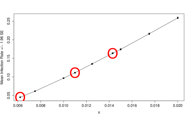
Figure 1: Mean infection rate as a function of $\pi$. These values were obtained by simulating the model described in Section 2 and varying the per-contact probability of HIV transmission. The underlying data are described in Section 3.1. The circles correspond to the values of $\pi$ chosen for the simulations and to calculate the new predictor of risk.

Summary statistics were calculated for the number of partners reported by the 466 participants. Summary statistics were also calculated for the estimated number of times participants reported that they had had sex over the previous six months. Using the notation of the previous section, for participant $i$, this value would be $\sum_{j=1}^{15}Z_{ij}$.

HIV incidence was estimated using the method described in [17]. The number of new infections between Wave 1 and Wave 2 was the numerator and the total number of days at risk was the denominator. This was converted into number of new infections per 100 person-years at-risk. For those testing negative at both Wave 1 and Wave 2, the number of days at-risk was the number of days between their Wave 1 and Wave 2 interviews. For those testing negative at Wave 1 but positive at Wave 2, the number of days at-risk was half the number of days between their Wave 1 and Wave 2 interviews.

3.3 Results

Participants reported having a median of 3 sex partners over the past six months (first quartile: 2; third quartile: 5). The median number of times they were estimated to have had sex over the past six months was 18 (first quartile: 8; third quartile: 30).

The AUC for model 1 (multiple logistic regression, Wave 1 outcome) was 0.5695; the AUC for model 2 (multiple logistic regression, Wave 2 outcome) was 0.5825; the AUC for model 3 (simple logistic regression, Wave 1 outcome) was 0.3978; and the AUC for model 4 (simple logistic regression, Wave 2 outcome) was 0.3978. Whether $\pi$ was set to $0.0062$, $0.0110$, or $0.0143$, predictor 5 (the new method) yielded an AUC of 0.4256. Among the 234 participants who were HIV-negative at Wave 1 and had HIV status data at Wave 2, seventeen tested positive at Wave 2. There was a total of 63,776.5 person-days at risk, yielding 0.0974 new infections per 100 person-years at-risk.

3.4 Discussion

The new risk estimator performs better than simple logistic regression using estimated number of sexual encounters as the single independent variable. Unfortunately, the new risk estimator performs worse than both chance and multiple logistic regression.

There are a number of potential reasons that this is the case. First, the venues listed are not actual venues but categories. They comprise many possible places where the men in the study could meet their sex partners. Two men who meet their sex partners exclusively on the internet could be doing so through two completely different websites. So, the data do not exactly map onto the proposed model. Second, men were asked about their sexual activity over the past six months. This is a long window of time, and even people with good memories are bound to make errors in estimating the number of times they had sex with a given person during that time period, or where they met. In other words, there is some measurement error. Third, a large number of participants met their partners through friends or already knew them, and these partners were not considered as potential sources of transmission. Fourth, the model assumes a constant probability of transmission for all serodiscordant couplings. In reality, some couplings will involve condoms, some will involve pre-exposure prophylaxis (PrEP), and some will be unprotected. Further mismatches between the model and the data include the sampling mechanism (the participants in the dataset were recruited through a version of respondent-driven sampling and were not selected uniformly at random from the population of Black MSM in Chicago); variable follow-up time across participants; and follow-up time (approximately nine months) not equaling the amount of time before Wave 1 for which participants were asked about their sex partners (six months).

Figure 2A demonstrates another explanation for the poor performance of the new risk estimator. It depicts the venue-to-venue graph, in which each node is a venue and two venues are connected by an edge if at least one participant met a sex partner at both venues. The width of the edge between two venues corresponds to the number of participants they share. It’s apparent from the figure that the venues are connected in one overarching cluster. The participants in the study have a lot of overlap in where they meet their partners, so they all have similar risks of contracting HIV.

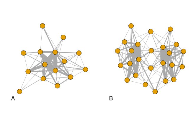
Figure 2: Venue-to-venue network. Each node is a venue, and two venues are connected by an edge if at least one participant met a sex partner at both venues. The width of the edge between two venues corresponds to the number of participants they share. (A) The original data set. (B) The modified data set used in Simulation Study 2.

Although the results are somewhat disappointing, our simulation approach is able to identify potential reasons for that, and there are actually good reasons to believe that the method might perform well in practice if the relevant data were available.

4 Simulation Study 1

We used simulation to evaluate the performance of the new method when the model is correct. As explained below, we tested the risk estimator when data collection is perfect; when venues are reported as grouped, even though they are distinct for the purpose of data generation; when some venues are not reported; and when venues are reported incorrectly.

4.1 Methods

Sample size $n$ was set to 466; population size $N$ was set to $n\times 5=$ 2,330; the population number of venues $M$ was set to 15; and $\pi$ was set first to 0.0062, then to 0.0110, and then to 0.0143. There were 1,000 replications for each value of $\pi$. If we consider each parameter vector to be $\left(\lambda_{i}p_{i1}t,\dotsc,\lambda_{i}p_{iM}t,Y_{i0}\right)^{\top}$, then for each replication, the $N$ parameter vectors were sampled uniformly at random with replacement from the 466 participants in the uConnect study. That is, each vector $\left(Z_{i1},\dotsc,Z_{i15},Y_{i0}\right)^{\top}$ from the previous section was considered to be a potential parameter vector $\left(\lambda_{i}p_{i1}t,\dotsc,\lambda_{i}p_{i15}t,Y_{i0}\right)^{\top}$ for the simulation study. Since the participants in the original study were asked about their sexual activity over the previous six months, $t$ was set to six months.

Each replication consisted of the following steps:

1. Draw the $N$ parameter vectors.

2. Simulate the model for six months.

3. Record $Z_{ij}$ and $Y_{i0}$.

4. Draw a sample of size $n$.

5. Calculate the $\hat{Q}_{j}$ and $\hat{R}_{i}$ based on the sample.

6. Simulate the model for six more months.

7. Test $\hat{R}_{i}$ and the four logistic regressions from the previous section as predictors of $Y_{it}$ for the participants in the sample. Also, measure the number of new infections per 100 person-years at-risk.

In addition to varying $\pi$, we varied the missingness with regards to the venues. That is, we tested the following scenarios:

1. Perfect sampling. In this scenario, no venues were intentionally excluded (although a venue could have been excluded from the sample if none of its patrons were sampled).

2. Coarse sampling. This scenario was intended to represent participants grouping different venues into categories instead of reporting them as separate. The venues were first ordered from most to least patronized (by $\sum_{i=1}^{N}Z_{ij}$); then, the first through third were considered one venue for the purpose of calculating $\hat{Q}$; the fourth through sixth were considered one venue; etc. In other words, we used

   $$\hat{Q}_{1} =\frac{\sum_{j=1}^{3}\sum_{i=1}^{n}Z_{ij}Y_{i0}}{\sum_{j=1}^{3}\sum_{i=1}^{n}Z_{ij}}\text{,}$$

   $$\hat{Q}_{2} =\frac{\sum_{j=4}^{6}\sum_{i=1}^{n}Z_{ij}Y_{i0}}{\sum_{j=4}^{6}\sum_{i=1}^{n}Z_{ij}}\text{,}$$

   etc.

3. Smallest venues missing. This scenario was intended to represent participants not reporting the smallest venues. For all five risk prediction methods, the three least-patronized venues were ignored.

4. Largest venues missing. This scenario was intended to represent participants not reporting the venues that led to the highest numbers of sexual contacts. For all five risk prediction methods, the three venues with the highest values of $\sum_{i=1}^{n}Z_{ij}$ were ignored.

5. Contaminated reporting. This scenario was intended to represent participants reporting the wrong venues. For the purpose of calculating all five risk estimators, 50% of person $i$’s encounters at each venue were redistributed uniformly at random across all venues.

4.2 Results

Across 1,000 replications, the mean first, second, and third quartiles of the number of encounters per person were $7$, $15$, and $27$, respectively. These values are taken only from the simulation with $\pi=0.0062$, but note that the value of $\pi$ does not affect the number of encounters per person.

AUCs are presented in Figure 3. Figure 3A displays the AUCs for $\pi=0.0062$, Figure 3B displays the AUCs for $\pi=0.0110$, and Figure 3C displays the AUCs for $\pi=0.0143$. In general, as $\pi$ increases, the variability of the performance decreases.

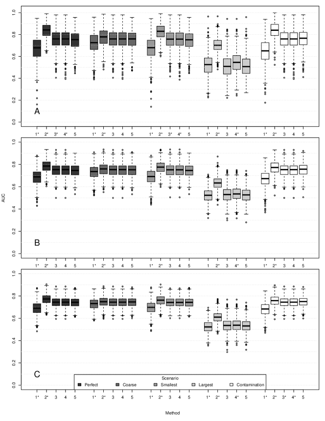
Figure 3: AUCs from 1,000 replications, single cluster. 1 = Multiple logistic regression trained on Wave 1 outcome; 2 = Multiple logistic regression trained on Wave 2 outcome; 3 = Simple logistic regression trained on Wave 1 outcome; 4 = Simple logistic regression trained on Wave 2 outcome; 5 = New method. An asterisk indicates that that method was significantly different from the new method at the 0.05 level. In panel (A) $\pi=0.0062$, in (B) $\pi=0.0110$, and in (C) $\pi=0.0143$.

For each value of $\pi$, and for the Perfect, Coarse, Smallest, and Contamination scenarios, multiple logistic regression trained on the Wave 1 outcome performs worst; simple logistic regression performs about the same as or slightly better than the new method, regardless of whether it is trained on the Wave 1 or Wave 2 outcome; and multiple logistic regression trained on the Wave 2 outcome performs best. For the Largest scenario, simple logistic regression trained on the Wave 1 outcome performs about the same as the new method; multiple logistic regression trained on the Wave 1 outcome performs about as well as simple logistic regression trained on the Wave 2 outcome; and multiple logistic regression trained on the Wave 2 outcome performs the best. In this missing data scenario, the AUCs for all methods are much lower than for other missing data scenarios.

4.3 Discussion

As $\pi$ decreases, new infections become more rare, making the relationship between the venues and the outcome more dependent on chance. This explains the increasing variability of the risk estimators with decreasing values of $\pi$.

The similarity of the performance of the new method with the simple logistic regressions seems to indicate that an individual’s pattern of venue visitation is not as important as his total number of sexual encounters. This is corroborated by the performance of the multiple logistic regressions, which seem to overfit the outcome to the data. This overfitting causes the multiple logistic regression trained on the Wave 1 outcome to display the worst performance and the multiple logistic regression trained on the Wave 2 outcome to display the best performance. Another piece of evidence for the primacy of number of sexual encounters is the Contamination scenario. Here, the reported pattern of venue visitation differs greatly from the true pattern of venue visitation, but each person’s total number of encounters remains the same. The performance of each method is about the same in this scenario as in the Perfect scenario, indicating that the total number of encounters is what matters. The Largest scenario provides a contrast to the Contamination scenario; here, the three venues with the most sexual encounters are not reported. This causes a decrease in the total number of sexual encounters reported by many participants, and the performance of all five risk estimators suffers.

The distribution of the number of sexual encounters per person is approximately the same in the simulation as in the dataset on which it is based.

5 Simulation Study 2

The following simulation study was intended to address the dense clustering of the venues demonstrated in Figure 2A. A new dataset was created, this time with two clusters and a much lower HIV prevalence in one of the clusters.

5.1 Methods

This simulation study was exactly the same as the first, with three exceptions. First, the 466 rows of the dataset were duplicated, generating a new dataset of 932 participants. For the second group of 466 participants, the ten largest venues were renamed. This meant there were 25 total venues, with the first 466 participants only overlapping with the second 466 participants at the five smallest venues. The resulting venue-to-venue graph is in Figure 2B. Second, this second group of participants was also modified in that each participant who was HIV-positive at Wave 1 was changed to be HIV-negative at Wave 1 with probability $0.75$. As a result, the second group had an HIV prevalence at Wave 1 of $0.0815$, whereas the first group had an HIV prevalence at Wave 1 of $0.3820$. Third, the population size $N$ was set to $932\times 5=4,660$. This new dataset formed the basis for the second simulation study in that in each replication, 862 participants were drawn uniformly at random from it.

5.2 Results

AUCs are presented in Figure 4. Figure 4A displays the AUCs for $\pi=0.0062$, Figure 4B displays the AUCs for $\pi=0.0110$, and Figure 4C displays the AUCs for $\pi=0.0143$. In general, as $\pi$ increases, the variability of the performance decreases.

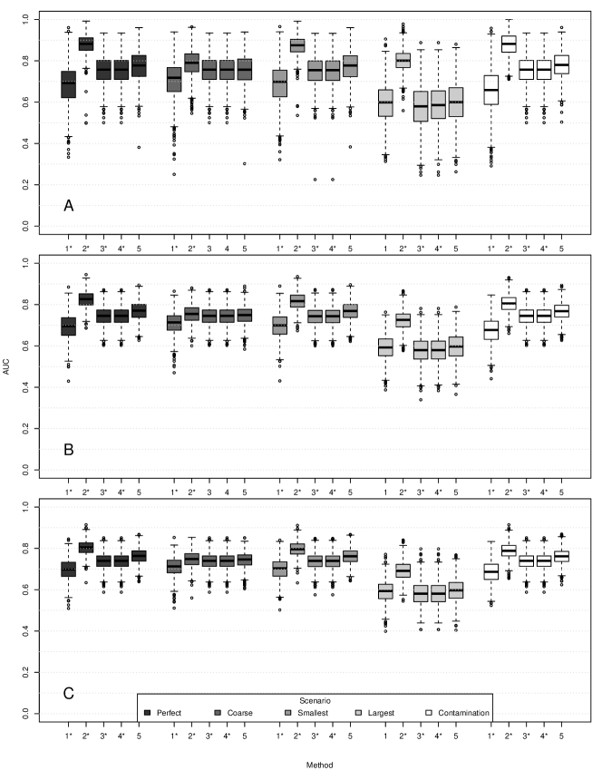
Figure 4: AUCs from 1,000 replications, two clusters. 1 = Multiple logistic regression trained on Wave 1 outcome; 2 = Multiple logistic regression trained on Wave 2 outcome; 3 = Simple logistic regression trained on Wave 1 outcome; 4 = Simple logistic regression trained on Wave 2 outcome; 5 = New method. An asterisk indicates that that method was significantly different from the new method at the 0.05 level. In panel (A) $\pi=0.0062$, in (B) $\pi=0.0110$, and in (C) $\pi=0.0143$.

For each value of $\pi$, and for the Perfect, Coarse, Smallest, and Contamination scenarios, multiple logistic regression trained on the Wave 1 outcome performs worst; simple logistic regression performs better; the new method performs even better; and multiple logistic regression trained on the Wave 2 outcome performs best. For the Largest scenario, the pattern is repeated except that multiple logistic regression trained on the Wave 1 outcome performs about as well as the new method. In this missing data scenario, the AUCs for all methods are much lower than for other missing data scenarios.

5.3 Discussion

The pattern of results for the Perfect, Coarse, Smallest, and Contamination scenarios for this simulation study differs from that for the previous simulation study in that the new method performs better than the two simple logistic regressions. This seems to indicate that the pattern of venue visitation is more relevant than the simple total number of sexual encounters per person. The superiority of the new method over multiple logistic regression trained on the Wave 1 outcome also indicates that the new method is not overfitting.

6 Discussion

This paper proposes a new model for HIV transmission based on where MSM meet their sexual partners, and tests a measure of risk based on that model in both real-world and simulated data. The measure of risk performs about as well as simple logistic regression when the venues where people meet their sex partners contains one large cluster, but performs better than both simple and multiple logistic regression when there are two clusters that differ in their HIV prevalence.

A plurality of the sex partners in the real-world sample were met through friends or were already known to the participants, and thus do not fit into the proposed model for HIV transmission. In order to account for that, this model could be extended by allowing people to be considered “venues.”

Admittedly, the assumption that sexual encounters follow a Poisson process is a strong one. It means that an individual’s rate of sexual encounters does not change over time, even if he finds out he has been infected with HIV. Gorbach, Javanbakht, and Bolan [18] found that the median number of partners among HIV-positive MSM in Los Angeles did decrease after diagnosis. That said, even if the newly-diagnosed men change their behavior, the model still uses information from men who already knew they were HIV-positive and from men who remain HIV-negative, and their behavior would not be expected to change. Also, the model is based on sampling from a population of MSM visiting these venues, so even if the sampled men change their behavior, the unsampled men may not. Finally, Gorbach, Javanbakht, and Bolan [18] found that the rate of condomless anal intercourse (CAI) among HIV-positive MSM did not decrease after diagnosis. Further studies may examine how this complex behavior change affects HIV risk for HIV-negative men in the same sexual network; the current paper is intended to be a starting point.

There are many ways to enrich this model. We ignored methods of protection such as condoms and pre-exposure prophylaxis (PrEP), as well as the fact that an HIV-positive person with undetectable viral load will not transmit the virus, even during unprotected sex. These realities can be incorporated into expansions of the model. We also ignored temporal patterns like people being more likely to attend bars and clubs on the weekends. However, if the interval $(-t,t)$ covers enough weeks, these temporal patterns may average out.

Although the proposed model was developed for HIV transmission in MSM, it does not need to be limited to this pathogen or this population. A natural extension is hepatitis in injection drug users (IDUs). Any IDU can share a needle with any other IDU without regard to gender, and IDUs may be restricted to meeting each other through a limited set of venues or drug dealers. Instead of sexual encounters, each IDU may have their own rate of injection drug use. An affiliation network of IDUs and hotels as sites of injection has already been created in Winnipeg [19].

7 Declarations

7.1 Ethics approval and consent to participate

As the authors obtained only de-identified data for this study, it was determined “not human subjects research” by the IRB of the Harvard T.H. Chan School of Public Health.

7.2 Availability of data and materials

The data that support the findings of this study are available from the uConnect Study Team [14, 5], but restrictions apply to the availability of these data, which were used under license for the current study, and so are not publicly available.

7.3 Declarations of interest

None.

7.4 Funding

Jonathan Larson is funded by NIH 2T32AI007358-31. Jukka-Pekka Onnela is funded by NIH R01AI138901. The uConnect study was funded by NIH R01DA033875. The funders had no role in study design; in the collection, analysis and interpretation of data; in the writing of the report; or in the decision to submit the article for publication.

7.5 Authors’ contributions

JL conceptualized and designed the study, conducted the analysis, and wrote the original draft. Both authors reviewed, edited, and approved the manuscript.

7.6 Acknowledgements

We would like to thank Lindsay Young, John Schneider, Stuart Michaels, Kayo Fujimoto, Hildie Cohen, and everyone on the uConnect team for sharing their data. We are also grateful for suggestions made by Alessandro Vespignani and Edoardo Airoldi.

8 Supplement

8.1 Empirical Study

8.1.1 Data

In the Wave 1 interview, participants were asked how often they had gone to clubs or bars; gyms; malls, shopping centers, or outdoor or public spaces; adult book stores or bathhouses; or ball scenes “to meet or socialize with other men”. The possible responses were “Every day”, “Several times a week”, “Once a week”, “Once every two weeks”, “Once a month”, “A couple of times a year”, “Once a year”, “Less than once a year”, and “Never”. For each of these venue types, participants were asked if they were located in the South Side, North Side, West Side, East Side, South Suburbs, or other part of Chicago. At Waves 1 and 2, participants received HIV tests and were asked about their HIV status. For the present analysis, HIV status was determined by lab results, unless those results were missing, in which case HIV status was determined by self-report.

In the Wave 1 data, 110 participants (18%) were missing lab HIV results and 43 (7%) were missing self-reported HIV status. Eight (1%) were missing both, and they were removed from the data set. Four participants (0.6%) were missing data on where they met or socialized with other men and were removed from the data set. One participant had the same date for his Wave 1 and Wave 2 interviews, and this date was neither the latest date for Wave 1 nor the earliest date for Wave 2. His Wave 2 data were deleted. This left 606 participants at Wave 1 (98.1% of the total) and 512 (82.8%) participants at Wave 2. Of the participants at Wave 2, 509 had HIV information.

The frequency data were recoded as follows to reflect number of visits to a venue type (e.g., clubs and bars) over the course of nine months, the average elapsed time between Wave 1 and Wave 2. Thus “Every day” became 270; “Several times a week” became 116, or three times per week; “Once a week” became 39; “Once every two weeks” became 19; “Once a month” became 9, “A couple of times a year” became 4; “Once a year” became 1; and “Less than once a year” and “Never” became 0. These values were then divided evenly across the neighborhoods the participant said he visited. For example, if a participant said he visited clubs and bars several times a week, and these clubs and bars were located on the North and South Sides, he was coded as visiting clubs and bars on the North Side 58 times and clubs and bars on the South Side 58 times. Two participants said they visited clubs and bars but didn’t know where, and one participant said he visited ball scenes but didn’t know where. These participants were not removed from the data set, but were coded as not visiting clubs and bars or ball scenes, respectively. Twenty-seven participants said they visited a venue type but did not state where. They were removed from the data set. This left 579 participants (93.7% of the total) at Wave 1 and 488 (79.0%) at Wave 2.

The median elapsed time between Wave 1 and Wave 2 was 267.5 days. Of the 362 participants who were HIV-negative at Wave 1, 293 had HIV status data at Wave 2.

A list of the venues and the estimated number of visits there across all participants in a nine-month period is in Table 2.

Venue	# Visits	%
Clubs and Bars, North Side	4,914	24.4
Clubs and Bars, East Side	290	1.4
Clubs and Bars, South Side	1,375	6.8
Clubs and Bars, West Side	237	1.2
Clubs and Bars, South Suburbs	213	1.1
Clubs and Bars, Other	305	1.5
Gyms, North Side	446	2.2
Gyms, East Side	61	0.3
Gyms, South Side	868	4.3
Gyms, West Side	237	1.2
Gyms, South Suburbs	24	0.1
Gyms, Other	98	0.5
Public Spaces, North Side	1,841	9.1
Public Spaces, East Side	407	2.0
Public Spaces, South Side	3,050	15.1
Public Spaces, West Side	1,251	6.2
Public Spaces, South Suburbs	1,087	5.4
Public Spaces, Other	123	0.6
Bathhouses and Bookstores, North Side	542	2.7
Bathhouses and Bookstores, East Side	38	0.2
Bathhouses and Bookstores, South Side	16	0.1
Bathhouses and Bookstores, West Side	291	1.4
Bathhouses and Bookstores, South Suburbs	1	0.0
Bathhouses and Bookstores, Other	21	0.1
Balls, North Side	402	2.0
Balls, East Side	112	0.6
Balls, South Side	1,350	6.7
Balls, West Side	434	2.2
Balls, South Suburbs	14	0.1
Balls, Other	0	0.0

Table 2: List of the venues in the final data set and the estimated number of visits to each venue.

8.1.2 Methods

We calculated five predictors of risk using data for the 30 venues included in the final data:

1. Multiple logistic regression based on Wave 1 HIV status:

   $$\operatorname{logit}E\left(Y_{i0}\right)=\beta_{0}+\beta_{1}Z_{i1}+\cdots+\beta_{30}Z_{i30}\text{.}$$

2. Multiple logistic regression based on Wave 2 HIV status:

   $$\operatorname{logit}E\left(Y_{it}\right)=\beta_{0}+\beta_{1}Z_{i1}+\cdots+\beta_{30}Z_{i30}\text{,}$$

   where $t$ indicates Wave 2.

3. Simple logistic regression based on Wave 1 HIV status:

   $$\operatorname{logit}E\left(Y_{i0}\right)=\beta_{0}+\beta_{1}\left(Z_{i1}+\cdots+Z_{i30}\right)\text{.}$$

4. Simple logistic regression based on Wave 2 HIV status:

   $$\operatorname{logit}E\left(Y_{it}\right)=\beta_{0}+\beta_{1}\left(Z_{i1}+\cdots+Z_{i30}\right)\text{,}$$

   where $t$ indicates Wave 2.

5. The new method. $\hat{Q}_{j}$, $1\leq j\leq 30$, was calculated as described above, and for each of the 293 participants who were HIV-negative at Wave 1 and had HIV status data at Wave 2, $\hat{R}_{i}$ was calculated. Three values of $\pi$ were tested: $0.62\%$, $1.1\%$, and $1.43\%$. Two of the values chosen for $\pi$ ($0.62\%$ and $1.43\%$) were selected from [16]. The lower, $0.62\%$, corresponds to the probability of transmission for insertive unprotected anal intercourse (UAI) in uncircumcised men. It was the second-lowest transmission rate reported in [16]; the lowest, $0.11\%$, led to replications with no new infections in the simulations described below. The upper value, $1.43\%$, corresponds to the probability of transmission for receptive UAI if ejaculation occurred inside the rectum. It was the highest transmission rate reported in [16]. The third value chosen for $\pi$ ($1.1\%$) was chosen because it led to an average of $0.1455$ new infections per 100 person-years at-risk, close to the value of $0.1193$ that was observed in the data. See Figure 5.

Estimators 1, 3, and 5, which trained on Wave 1 HIV status, used data from all 579 participants; estimators 2 and 4, which trained on Wave 2 HIV status, used data from the 485 participants who had Wave 2 HIV status. The estimators trained on Wave 2 HIV status are intended to give an upper bound to performance. Given that they are based on future knowledge, which would never be available to an investigator or clinician trying to estimate risk for a patient, they are not truly fair comparators. For each estimator, the AUC was calculated using the 293 participants who were HIV-negative at Wave 1 and had HIV status at Wave 2.

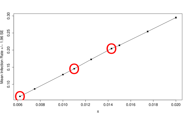
Figure 5: Mean infection rate as a function of $\pi$. These values were obtained by simulating the model described in Section 2 and varying the per-contact probability of HIV transmission. The underlying data are described in Section 8.1.1. The circles correspond to the values of $\pi$ chosen for the simulations and to calculate the new predictor of risk.

Summary statistics were also calculated for the estimated number of times participants reported that went somewhere to meet or socialize with other men. Using the notation of the previous section, for participant $i$, this value would be $\sum_{j=1}^{15}Z_{ij}$.

HIV incidence was estimated using the method described in [17]. The number of new infections between Wave 1 and Wave 2 was the numerator and the total number of days at risk was the denominator. This was converted into number of new infections per 100 person-years at-risk. For those testing negative at both Wave 1 and Wave 2, the number of days at-risk was the number of days between their Wave 1 and Wave 2 interviews. For those testing negative at Wave 1 but positive at Wave 2, the number of days at-risk was half the number of days between their Wave 1 and Wave 2 interviews.

8.1.3 Results

Participants reported making a median of 10 visits to one of the 30 venues in order to meet or socialize with other men (first quartile: 4; third quartile: 39).

The AUC for model 1 (multiple logistic regression, Wave 1 outcome) was 0.4850; the AUC for model 2 (multiple logistic regression, Wave 2 outcome) was 0.5990; the AUC for model 3 (simple logistic regression, Wave 1 outcome) was 0.5889; and the AUC for model 4 (simple logistic regression, Wave 2 outcome) was 0.5889. Whether $\pi$ was set to $0.0062$, $0.0110$, or $0.0143$, predictor 5 (the new method) yielded an AUC of 0.4092. Among the 293 participants who were HIV-negative at Wave 1 and had HIV status data at Wave 2, sixteen tested positive at Wave 2. There was a total of 79,614.5 person-days at risk, yielding 0.1193 new infections per 100 person-years at-risk.

8.1.4 Discussion

The new risk estimator performs worse than both chance and logistic regression. There are a number of potential reasons that this is the case. First, the venues listed are not actual venues but category-neighborhood combinations. Each comprises multiple possible places where the men in the study could meet their sex partners. So, the data do not exactly map onto the proposed model. Second, men were asked to estimate how often they visited each category of venue. This estimate is bound to involve error, and that error is compounded by the fact that categorical responses were translated into integer values. Third, the participants were asked about where they met or socialized with other men, not where they met their sex partners. Fourth, the model assumes a constant probability of transmission for all serodiscordant couplings. In reality, some couplings will involve condoms, some will involve pre-exposure prophylaxis (PrEP), and some will be unprotected. Further mismatches between the model and the data include the sampling mechanism (the participants in the dataset were recruited through a version of respondent-driven sampling and were not selected uniformly at random from the population of Black MSM in Chicago); and variable follow-up time across participants.

Figure 6 demonstrates another explanation for the poor performance of the new risk estimator. It depicts the venue-to-venue graph, in which each node is a venue and two venues are connected by an edge if at least one participant visited both. The width of the edge between two venues corresponds to the number of participants they share. It’s apparent from the figure that the venues are connected in one overarching cluster. The participants in the study have a lot of overlap in where they meet their partners, so they all have similar risks of contracting HIV.

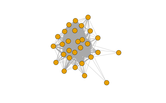
Figure 6: Venue-to-venue network for the original data. Each node is a venue, and two venues are connected by an edge if at least one participant visited both. The width of the edge between two venues corresponds to the number of participants they share.

Although the results are somewhat disappointing, our simulation approach is able to identify potential reasons for that, and there are actually good reasons to believe that the method might perform well in practice if the relevant data were available.

8.2 Simulation Study 1

We used simulation to evaluate the performance of the new method when the model is correct. What were visits to a venue in the empirical data study became sexual encounters in this simulation. As explained below, we tested the risk estimator when data collection is perfect; when venues are reported as grouped, even though they are distinct for the purpose of data generation; when some venues are not reported; and when venues are reported incorrectly.

8.2.1 Methods

Sample size $n$ was set to 579; population size $N$ was set to $n\times 5=$ 2,895; the population number of venues $M$ was set to 30; and $\pi$ was set first to 0.0062, then to 0.0110, and then to 0.0143. There were 1,000 replications for each value of $\pi$. If we consider each parameter vector to be $\left(\lambda_{i}p_{i1}t,\dotsc,\lambda_{i}p_{iM}t,Y_{i0}\right)^{\top}$, then for each replication, the $N$ parameter vectors were sampled uniformly at random with replacement from the 579 participants in the uConnect study. That is, each vector $\left(Z_{i1},\dotsc,Z_{i15},Y_{i0}\right)^{\top}$ from the previous section was considered to be a potential parameter vector $\left(\lambda_{i}p_{i1}t,\dotsc,\lambda_{i}p_{i15}t,Y_{i0}\right)^{\top}$ for the simulation study. Since the participants in the original study were asked about their sexual activity over the previous six months, $t$ was set to six months.

Each replication consisted of the following steps:

1. Draw the $N$ parameter vectors.

2. Simulate the model for nine months.

3. Record $Z_{ij}$ and $Y_{i0}$.

4. Draw a sample of size $n$.

5. Calculate the $\hat{Q}_{j}$ and $\hat{R}_{i}$ based on the sample.

6. Simulate the model for nine more months.

7. Test $\hat{R}_{i}$ and the four logistic regressions from the previous section as predictors of $Y_{it}$ for the participants in the sample. Also, measure the number of new infections per 100 person-years at-risk.

In addition to varying $\pi$, we varied the missingness with regards to the venues. That is, we tested the following scenarios:

1. Perfect sampling. In this scenario, no venues were intentionally excluded (although a venue could have been excluded from the sample if none of its patrons were sampled).

2. Coarse sampling. This scenario was intended to represent participants grouping different venues into categories instead of reporting them as separate. The venues were first ordered from most to least patronized (by $\sum_{i=1}^{N}Z_{ij}$); then, the first through third were considered one venue for the purpose of calculating $\hat{Q}$; the fourth through sixth were considered one venue; etc. In other words, we used

   $$\hat{Q}_{1} =\frac{\sum_{j=1}^{3}\sum_{i=1}^{n}Z_{ij}Y_{i0}}{\sum_{j=1}^{3}\sum_{i=1}^{n}Z_{ij}}\text{,}$$

   $$\hat{Q}_{2} =\frac{\sum_{j=4}^{6}\sum_{i=1}^{n}Z_{ij}Y_{i0}}{\sum_{j=4}^{6}\sum_{i=1}^{n}Z_{ij}}\text{,}$$

   etc.

3. Smallest venues missing. This scenario was intended to represent participants not reporting the smallest venues. For all five risk prediction methods, the three least-patronized venues were ignored.

4. Largest venues missing. This scenario was intended to represent participants not reporting the venues that led to the highest numbers of sexual contacts. For all five risk prediction methods, the three venues with the highest values of $\sum_{i=1}^{n}Z_{ij}$ were ignored.

5. Contaminated reporting. This scenario was intended to represent participants reporting the wrong venues. For the purpose of calculating all five risk estimators, 50% of person $i$’s encounters at each venue were redistributed uniformly at random across all venues.

8.2.2 Results

Across 1,000 replications, the mean first, second, and third quartiles of the number of visits per person were $1.9$, $11.2$, and $33.2$, respectively. These values are taken only from the simulation with $\pi=0.0062$, but note that the value of $\pi$ does not affect the number of encounters per person.

AUCs are presented in Figure 7. Figure 7A displays the AUCs for $\pi=0.0062$, Figure 7B displays the AUCs for $\pi=0.0110$, and Figure 7C displays the AUCs for $\pi=0.0143$. In general, as $\pi$ increases, the variability of the performance decreases.

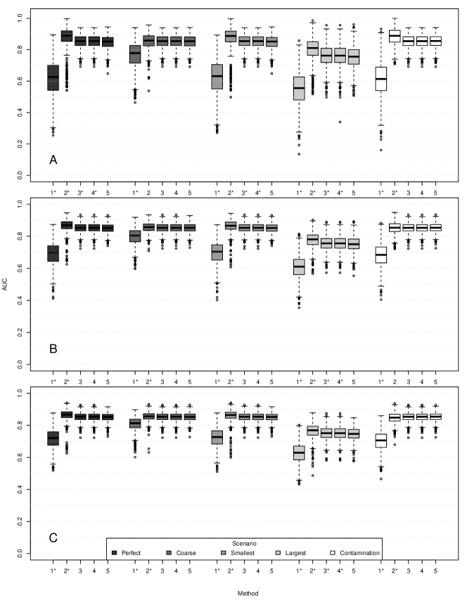
Figure 7: AUCs from 1,000 replications, single cluster. 1 = Multiple logistic regression trained on Wave 1 outcome; 2 = Multiple logistic regression trained on Wave 2 outcome; 3 = Simple logistic regression trained on Wave 1 outcome; 4 = Simple logistic regression trained on Wave 2 outcome; 5 = New method. An asterisk indicates that that method was significantly different from the new method at the 0.05 level (two-sided). In panel (A) $\pi=0.0062$, in (B) $\pi=0.0110$, and in (C) $\pi=0.0143$.

For each value of $\pi$ and in each scenario, multiple logistic regression trained on the Wave 1 outcome performs worst; simple logistic regression performs about as well as or slightly better than the new method, regardless of whether it is trained on the Wave 1 or Wave 2 outcome; and multiple logistic regression trained on the Wave 2 outcome performs best.

8.2.3 Discussion

As $\pi$ decreases, new infections become more rare, making the relationship between the venues and the outcome more dependent on chance. This explains the increasing variability of the risk estimators with decreasing values of $\pi$.

The similarity of the performance of the new method with the simple logistic regressions seems to indicate that an individual’s pattern of venue visitation is not as important as his total number of sexual encounters. This is corroborated by the performance of the multiple logistic regressions, which seem to overfit the outcome to the data. This overfitting causes the multiple logistic regression trained on the Wave 1 outcome to display the worst performance and the multiple logistic regression trained on the Wave 2 outcome to display the best performance. Another piece of evidence for the primacy of number of sexual encounters is the Contamination scenario. Here, the reported pattern of venue visitation differs greatly from the true pattern of venue visitation, but each person’s total number of encounters remains the same. The performance of each method is about the same in this scenario as in the Perfect scenario, indicating that the total number of encounters is what matters. The Largest scenario provides a contrast to the Contamination scenario; here, the three venues with the most sexual encounters are not reported. This causes a decrease in the total number of sexual encounters reported by many participants, and the performance of all five risk estimators suffers.

The distribution of the number of venue visits per person is approximately the same in the simulation as in the dataset on which it is based.

8.3 Simulation Study 2

The following simulation study was intended to address the dense clustering of the venues demonstrated in Figure 2. A new dataset was created, this time with two clusters and a much lower HIV prevalence in one of the clusters.

8.3.1 Methods

This simulation study was exactly the same as the first, with three exceptions. First, the 579 rows of the dataset were duplicated, generating a new dataset of 1158 participants. For the second group of 579 participants, the ten largest venues were renamed. This meant there were 40 total venues, with the first 579 participants only overlapping with the second 579 participants at the twenty smallest venues. Second, this second group of participants was also modified in that each participant who was HIV-positive at Wave 1 was changed to be HIV-negative at Wave 1 with probability $0.75$. As a result, the second group had an HIV prevalence at Wave 1 of $0.0898$, whereas the first group had an HIV prevalence at Wave 1 of $0.3748$. Third, the population size $N$ was set to $1158\times 5=5790$. This new dataset formed the basis for the second simulation study in that in each replication, 1158 participants were drawn uniformly at random from it.

8.3.2 Results

AUCs are presented in Figure 8. Figure 8A displays the AUCs for $\pi=0.0062$, Figure 8B displays the AUCs for $\pi=0.0110$, and Figure 8C displays the AUCs for $\pi=0.0143$. In general, as $\pi$ increases, the variability of the performance decreases.

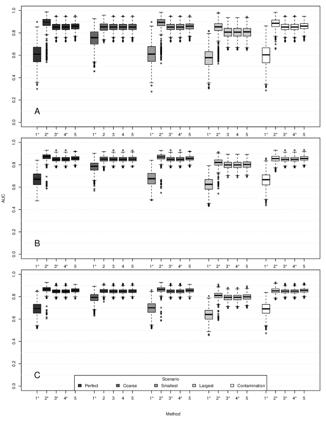
Figure 8: AUCs from 1,000 replications, two clusters. 1 = Multiple logistic regression trained on Wave 1 outcome; 2 = Multiple logistic regression trained on Wave 2 outcome; 3 = Simple logistic regression trained on Wave 1 outcome; 4 = Simple logistic regression trained on Wave 2 outcome; 5 = New method. An asterisk indicates that that method was significantly different from the new method at the 0.05 level. In panel (A) $\pi=0.0062$, in (B) $\pi=0.0110$, and in (C) $\pi=0.0143$.

For each value of $\pi$ and each scenario, multiple logistic regression trained on the Wave 1 outcome performs worst; simple logistic regression performs about as well as or slightly worse than the new method, regardless of whether it is trained on the Wave 1 or Wave 2 outcome; and multiple logistic regression trained on the Wave 2 outcome performs best.

8.3.3 Discussion

The pattern of results differs from that for the previous simulation study in that the new method performs better than the two simple logistic regressions. This seems to indicate that the pattern of venue visitation is more relevant than the simple total number of sexual encounters per person. The superiority of the new method over multiple logistic regression trained on the Wave 1 outcome also indicates that the new method is not overfitting.

References

- [1] HIV Surveillance Report, 2018 (Updated). Centers for Disease Control and Prevention; 2020. 31. Accessed 2021-04-19. Available from: http://www.cdc.gov/hiv/library/reports/hiv-surveillance.html.
- [2] Beyrer C, Baral SD, Walker D, Wirtz AL, Johns B, Sifakis F. The expanding epidemics of HIV Type 1 among men who have sex with men in low- and middle-income countries: Diversity and consistency. Epidemiol Rev. 2010;32:137–151.
- [3] Millett GA, Peterson JL, Flores SA, Hart TA, Jeffries WLt, Wilson PA, et al. Comparisons of disparities and risks of HIV infection in black and other men who have sex with men in Canada, UK, and USA: A meta-analysis. Lancet. 2012;380:341–348.
- [4] Jones J, Hoenigl M, Siegler AJ, Sullivan S P S Little, Rosenberg E. Assessing the performance of 3 human immunodeficiency virus incidence risk scores in a cohort of black and white men who have sex with men in the South. Sex Transm Dis. 2017;44:297–302.
- [5] Lancki N, Almirol E, Alon L, McNulty M, Schneider JA. Preexposure prophylaxis guidelines have low sensitivity for identifying seroconverters in a sample of young Black MSM in Chicago. AIDS. 2018;32:383–392.
- [6] Raymond HF, McFarland W. Racial mixing and HIV risk among men who have sex with men. AIDS Behav. 2009;13:630–637.
- [7] Glick SN, Morris M, Foxman B, Aral SO, Manhart LE, Holmes KK, et al. A comparison of sexual behavior patterns among men who have sex with men and heterosexual men and women. J Acquir Immune Defic Syndr. 2012;60:83–90.
- [8] Jennings JM, Reilly ML, Perin J. Sex partner meeting places over time among newly HIV-diagnosed men who have sex with men in Baltimore, Maryland. Sex Transm Dis. 2015;42:549–553.
- [9] Oster AM, Wejnert C, Mena LA, Elmore K, Fisher H, Heffelfinger JD. Network analysis among HIV-infected young black men who have sex with men demonstrates high connectedness around few venues. Sex Transm Dis. 2013;40:206–212.
- [10] Fujimoto K, Williams M, Ross MW. Venue-based affiliation networks and HIV risk-taking behavior among male sex workers. Sex Transm Dis. 2013;40:453–458.
- [11] Holloway IW, Rice E, Kipke MD. Venue-based network analysis to inform HIV prevention efforts among young gay, bisexual, and other men who have sex with men. Prev Sci. 2014;15:419–427.
- [12] Leung KK, Poon CM, S LS. A comparative analysis of behaviors and sexual affiliation networks among men who have sex with men in Hong Kong. Arch Sex Behav. 2015;44:2067–2076.
- [13] Brantley M, Schumacher C, Fields EL, Perin J, Safi AG, Ellen J, et al. The network structure of sex partner meeting places reported by HIV-infected MSM: Opportunities for HIV targeted control. Soc Sci Med. 2017;182:20–29.
- [14] Young LE, Michaels S, Jonas A, Khanna AS, Skaathun B, Morgan E, et al. Sex behaviors as social cues motivating social venue patronage among young black men who have sex with men. AIDS Behav. 2017;21:2924–2934.
- [15] Chan PA, Crowley C, Rose J, Kershaw T, Tributino A, Montgomery MC, et al. A network analysis of sexually transmitted diseases and online hookup sites among men who have sex with men. Sex Transm Dis. 2018;45:462–468.
- [16] Jin F, Jansson J, Law M, Prestage GP, Zablotska I, Imrie JC, et al. Per-contact probability of HIV transmission in homosexual men in Sydney in the era of HAART. AIDS. 2010;24:907–913.
- [17] Neaigus A, Jenness SM, Hagan H, Murrill CS, Torian LV, Wendel T, et al. Estimating HIV incidence and the correlates of recent infection in venue-sampled men who have sex with men in New York City. AIDS Behav. 2012;16:516–524.
- [18] Gorbach PM, Javanbakht M, Bolan RK. Behavior change following HIV diagnosis: Findings from a cohort of Los Angeles MSM. AIDS Care. 2018;30:300–304.
- [19] Wylie JL, Shah L, Jolly A. Incorporating geographic settings into a social network analysis of injection drug use and bloodborne pathogen prevalence. Health Place. 2007;13:617–628.