Tunneling in Fermi Systems with Quadratic Band Crossing Points

Abstract

We investigate the tunneling of quasiparticles through a rectangular potential barrier of finite height and width, in 2d and 3d semimetals with band structures consisting of a quadratic band crossing point. We compute the transmission coefficient at various incident angles, and also demonstrate the behaviour of the conductivity and the Fano factor. We discuss the distinguishing signatures of these transport properties in comparison with other semimetals, as well as electrons in normal metals.

I Introduction

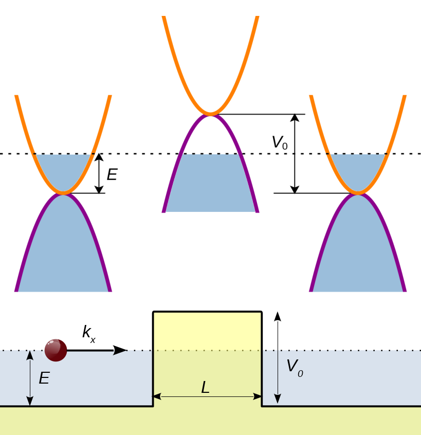
Figure 1: Tunneling through a potential barrier in a QBCP material. The upper panel shows the schematic diagrams of the spectrum of quasiparticles about a QBCP, with respect to a potential barrier in the $x$-direction. The lower panel represents the schematic diagram of the transport across the potential barrier. The Fermi level (indicated by dotted lines) lies in the conduction band outside the barrier, and in the valence band inside it. The blue fillings indicate occupied states.

Multiband fermionic systems may exhibit a band crossing point in the Brillouin zone where two or more bands cross. If the chemical potential is adjusted to lie exactly at that point, the Fermi surface shrinks to a Fermi node. The most famous example of such a Fermi node is the case of a linear band crossing, whose low energy properties are described by Dirac fermions, and are conspicuous in systems like nodal superconductors and graphene. In this paper, we consider systems with a quadratic band crossing point (QBCP) somewhere in their two-dimensional (2d) [1, 2, 3] or three-dimensional (3d) [4, 5, 6] Brillouin zones. 2d QBCPs can be realised in checkerboard [1] (at $1/2$ filling), Kagome [1] (at $1/3$ filling), and Lieb [2] lattices. On the other hand, pyrochlore iridates $\text{A}_{2}\text{Ir}_{2}\text{O}_{7}$ (A is a lanthanide element [7, 8]) have been shown to host a 3d QBCP. Such bandstructures have also been realised in 3d gapless semiconductors in the presence of a sufficiently strong spin-orbit coupling [9], such that the resulting model of a semimetal is indeed relevant for materials like gray tin ($\alpha$-Sn) and mercury telluride (HgTe). These systems are also known as “Luttinger semimetals” [10] due to the fact that the low-energy fermionic degrees of freedom are captured by the Luttinger Hamiltonian of inverted band-gap semiconductors [11, 12].

Our aim is to compute the tunneling coefficients and other transport characteristics when the quasiparticles of the QBCP semimetals are subjected to a potential barrier of finite strength and width along one direction, which is chosen to be the $x$-axis. This scenario is represented in the cartoon in Fig. 1. Our results will show how these transport characteristics are significantly different from those in normal metals, due to the presence of multiple bands. We will also compare their features with those of other semimetals like graphene, bilayer graphene and three-band pseudospin-$1$ systems.

The paper is organized as follows. In Sec. II, we study the 2d QBCPs, while Sec. III deals with the 3d QBCP case. We compare our findings with the results for some other known bandstructures in Sec. IV. Finally, we end with a summary and outlook in Sec. V.

II 2d Model

For a 2d system, the particle-hole symmetric QBCP with $C_{6}$ rotational symmetry is described by the Hamiltonian [1]:

$$\mathcal{H}_{2d}^{kin}(k_{x},k_{y}) =\frac{\hbar^{2}}{2\,m}\Big{[}\,2\,k_{x}\,k_{y}\,\sigma_{x}+\left(k_{y}^{2}-k_{x}^{2}\right)\sigma_{z}\,\Big{]}$$ (1)

in the momentum space, with eigenvalues

$$\varepsilon_{2d}^{\pm}(k_{x},k_{y})=\pm\frac{\hbar^{2}\left(k_{x}^{2}+k_{y}^{2}\right)}{2\,m},$$ (2)

where the “$+$” and “$-$” signs, as usual, refer to the conduction and valence bands respectively. The corresponding eigenvectors are given by:

$$\Psi_{+}=\frac{1}{\sqrt{k_{x}^{2}+k_{y}^{2}}}\{k_{y},k_{x}\}\,,\text{ and }\Psi_{-}=\frac{1}{\sqrt{k_{x}^{2}+k_{y}^{2}}}\{-k_{x},k_{y}\},$$ (3)

respectively.

The 2d system is modulated by a square electric potential barrier of height $V_{0}$ and width $L$, giving rise to an $x$-dependent potential energy function:

$$V(x)=\begin{cases}V_{0}&\text{ for }0<x<L\\ 0&\text{ otherwise}\,.\end{cases}$$ (4)

Hence, we need to consider the total Hamiltonian:

$$\mathcal{H}_{2d}^{tot} =\mathcal{H}_{2d}^{kin}(-\mathrm{i}\,\partial_{x},-\mathrm{i}\,\partial_{y})+V(x)$$ (5)

in position space. We choose the $x$-axis along the transport direction, and place the chemical potential at an energy $E>0$ in the region outside the potential barrier. The Fermi energy $E$ can in general be tuned by chemical doping or a gate voltage.

II.1 Formalism

For a material of a sufficiently large transverse dimension $W$, the boundary conditions should be irrelevant for the bulk response, and we use this freedom to simplify the calculation. Here, on a physical wavefunciton $\Psi^{\mathrm{tot}}$ we impose periodic boundary conditions:

$$\Psi^{\mathrm{tot}}(x,W)=\Psi^{\mathrm{tot}}(x,0)\,.$$ (6)

The transverse momentum $k_{y}$ is conserved, and it is quantized due to the periodicity in the transverse width $W$, and hence takes the form:

$$\quad k_{y}=\frac{2\,\pi\,n}{W}\equiv q_{n}\,,$$ (7)

where $n\in\mathbb{Z}$. For the longitudinal direction, we seek plane wave solutions of the form $e^{\mathrm{i}\,k_{x}x}$. Then the full wavefunction is given by:

$$\Psi^{\mathrm{tot}}(x,y,n)=\text{const.}\times\Psi_{n}(x)\,e^{\mathrm{i}\,q_{n}y}\,,$$ (8)

For any mode of given transverse momentum component $k_{y}$, we can determine the $x$-component of the wavevectors of the incoming, reflected, and transmitted waves (denoted by $k_{\ell}$), by solving $\varepsilon_{2d}^{\pm}(k_{x},n)=\pm\frac{\hbar^{2}\left(k_{\ell}^{2}+q_{n}^{2}\right)}{2\,m}\,.$ In the regions $x<0$ and $x>L$, we have only propagating modes ($k_{\ell}$ is real), while the $x$-components in the scattering region (denoted by $\tilde{k}$), are given by $\tilde{k}^{2}=\frac{2\,m\,|E-V_{0}|}{\hbar^{2}}-q_{n}^{2}$, and may be propagating (imaginary part of $\tilde{k}$ is zero) or evanescent (imaginary part of $\tilde{k}$ is nonzero).

We will follow the procedure outlined in Refs. 13, 14 to compute the transport coefficients. We consider the transport of positive energy states ($\Psi_{+}$) corresponding to electron-like particles. The transport of hole-like excitations ($\Psi_{-}$) will be similar. Hence, the Fermi level outside the potential barrier is adjusted to a value $E=\varepsilon_{2d}^{+}(k_{x},k_{y})$. Such a scattering state $\Psi_{n,+}$, in the mode labeled by $n$, is constructed from the states:

$$\Psi_{n}(x)= \begin{cases}\phi_{L}&\text{ for }x<0\,,\\ \phi_{M}&\text{ for }0<x<L\,,\\ \phi_{R}&\text{ for }x>L\,,\end{cases}$$

$$\phi_{L}= \,\frac{\Psi_{+}(k_{\ell},q_{n})\,e^{\mathrm{i}\,k_{\ell}x}+r_{n}\,\Psi_{+}(-k_{\ell},q_{n})\,e^{-\mathrm{i}\,k_{\ell}x}}{\sqrt{\mathcal{V}(k_{\ell},n)}}\,,$$

$$\phi_{M}= \,\Big{[}\alpha_{n}\,\Psi_{+}(\tilde{k},q_{n})\,e^{\mathrm{i}\,\tilde{k}\,x}+\beta_{n}\,\Psi_{+}(-\tilde{k},q_{n})\,e^{-\mathrm{i}\,\tilde{k}\,x}\Big{]}\,\Theta\left(E-V_{0}\right)+\Big{[}\alpha_{n}\,\Psi_{-}(\tilde{k},q_{n})\,e^{\mathrm{i}\,\tilde{k}\,x}+\beta_{n}\,\Psi_{-}(-\tilde{k},q_{n})\,e^{-\mathrm{i}\,\tilde{k}\,x}\Big{]}\,\Theta\left(V_{0}-E\right),$$

$$\phi_{R}= \,t_{n}\,\Psi_{+}(k_{\ell},q_{n})\,\frac{e^{\mathrm{i}\,k_{\ell}\left(x-L\right)}}{\sqrt{\mathcal{V}(k_{\ell},n)}}\,,$$

$$\mathcal{V}(k_{\ell},n)\equiv \,|\partial_{k_{\ell}}\varepsilon_{+}(k_{\ell},n)|=\frac{\hbar^{2}k_{\ell}}{m}\,,\quad k_{\ell}=\sqrt{\frac{2\,m\,E}{\hbar^{2}}-q_{n}^{2}}\,,\quad\tilde{k}=\sqrt{\frac{2\,m\,|E-V_{0}|}{\hbar^{2}}-q_{n}^{2}}\,,$$ (9)

where we have used the velocity $\mathcal{V}(k_{\ell},n)$ to normalize the incident, reflected and transmitted plane waves. Note that for $V_{0}>E$, the Fermi level within the potential barrier lies within the valence band, and we must use the valence band wavefunctions in that region.

The boundary conditions can be obtained by integrating the equation $\mathcal{H}_{2d}^{tot}\,\Psi^{\mathrm{tot}}=E\,\Psi^{\mathrm{tot}}$ over a small interval in the $x$-direction around the points $x=0$ and $x=L$. The results are that the two components of the wavefunction be continuous at the boundaries. These conditions are sufficient to guarantee the continuity of the current flux along the $x$-direction . In particular, the reflection and transmission amplitudes $r_{n},t_{n}$, and the two coefficients $\left(\alpha_{n},\beta_{n}\right)$, are determined from these boundary conditions. This mode-matching procedure gives us:

$$r_{n}(E,V_{0}) =\begin{cases}\frac{\left(\tilde{k}^{2}k_{\ell}^{2}-q_{n}^{4}\right)\sin(\tilde{k}L)}{\left(\tilde{k}^{2}k_{\ell}^{2}+q_{n}^{4}\right)\sin(\tilde{k}L)-2\,\mathrm{i}\,\tilde{k}\,k_{\ell}\,q_{n}^{2}\cos(\tilde{k}L)}&\text{ for }E<V_{0}\\ \frac{\left(k_{\ell}^{2}-\tilde{k}^{2}\right)\sin\left(\tilde{k}L\right)}{\left(\tilde{k}^{2}+\,k_{\ell}^{2}\right)\sin\left(\tilde{k}L\right)+2\,\mathrm{i}\,\tilde{k}\,\,k_{\ell}\cos\left(\tilde{k}L\right)}&\text{ for }E>V_{0}\,.\end{cases}$$ (10)

and

$$t_{n}(E,V_{0}) =\begin{cases}-\frac{2\,\mathrm{i}\,\tilde{k}\,k_{\ell}\,q_{n}^{2}}{\left(\tilde{k}^{2}\,k_{\ell}^{2}+q_{n}^{4}\right)\sin\left(\tilde{k}L\right)-2\,\mathrm{i}\,\tilde{k}\,k_{\ell}\,q_{n}^{2}\cos\left(\tilde{k}L\right)}&\text{ for }E<V_{0}\\ \frac{2\,\mathrm{i}\,\tilde{k}\,k_{\ell}}{\left(\tilde{k}^{2}+\,k_{\ell}^{2}\right)\sin\left(\tilde{k}L\right)+2\,\mathrm{i}\,\tilde{k}\,\,k_{\ell}\cos\left(\tilde{k}L\right)}&\text{ for }E>V_{0}\,.\end{cases}$$ (11)

The reflection and transmission coefficients at an energy $E$ are given by

$$R(E,V_{0},\phi)=|r_{n}(E,V_{0})|^{2}\text{ and }T(E,V_{0},\phi)=|t_{n}(E,V_{0})|^{2}\,,$$ (12)

respectively, where $\phi=\tan^{-1}\left(\frac{q_{n}}{k_{\ell}}\right)$ is the incident angle of the incoming wave.

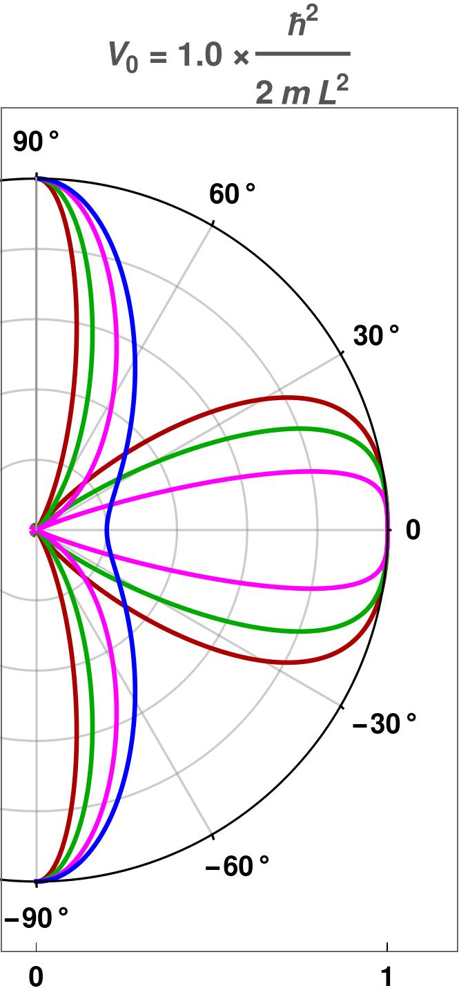
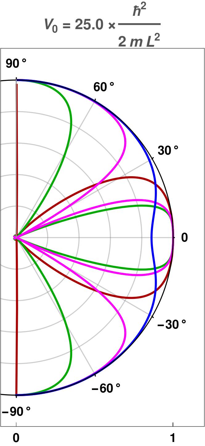
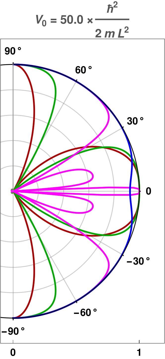
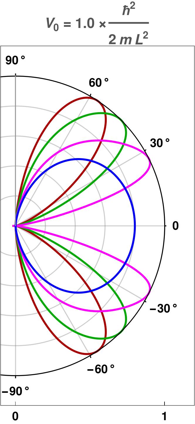
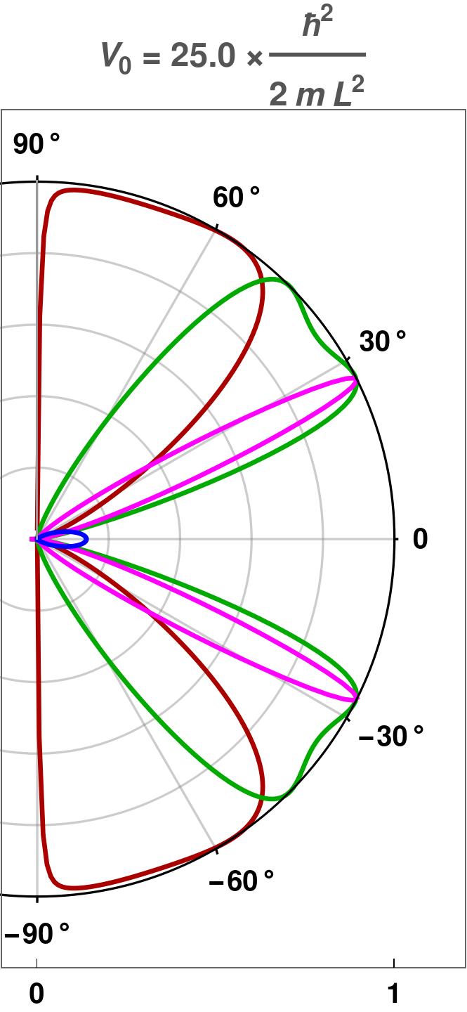
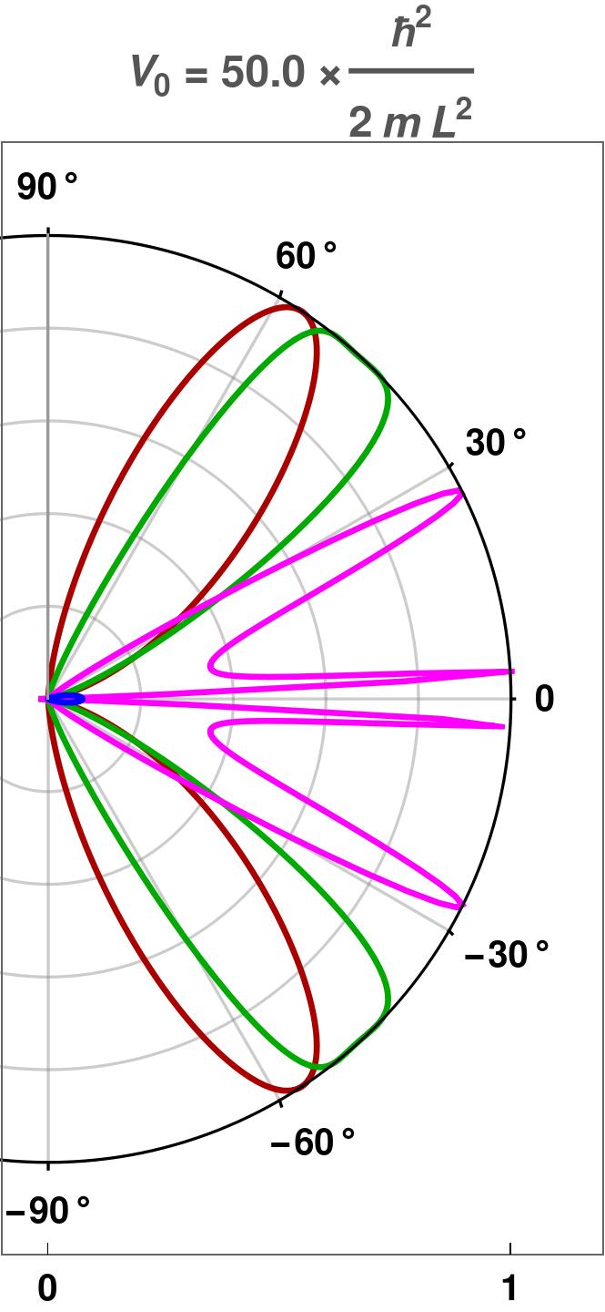
Figure 2: 2d QBCP: The polar plots show the reflection coefficient $R(E,V_{0},\phi)\big{|}_{E\leq V_{0}}$ and the transmission coefficient $T(E,V_{0},\phi)\big{|}_{E\leq V_{0}}$ as functions of the incident angle $\phi$ for the parameters $E=0.3\,V_{0}$ (red), $E=0.5\,V_{0}$ (green), $E=0.8\,V_{0}$ (magenta) and $E=1.0\,V_{0}$ (blue).

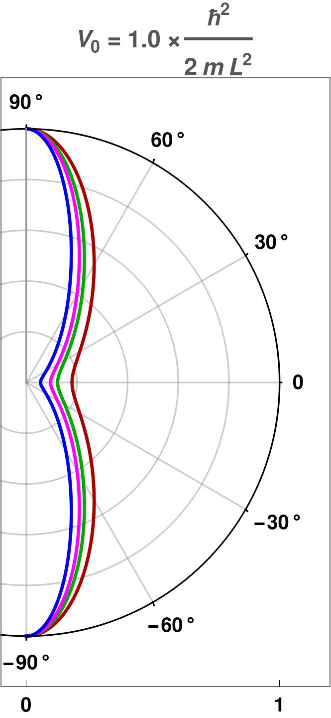
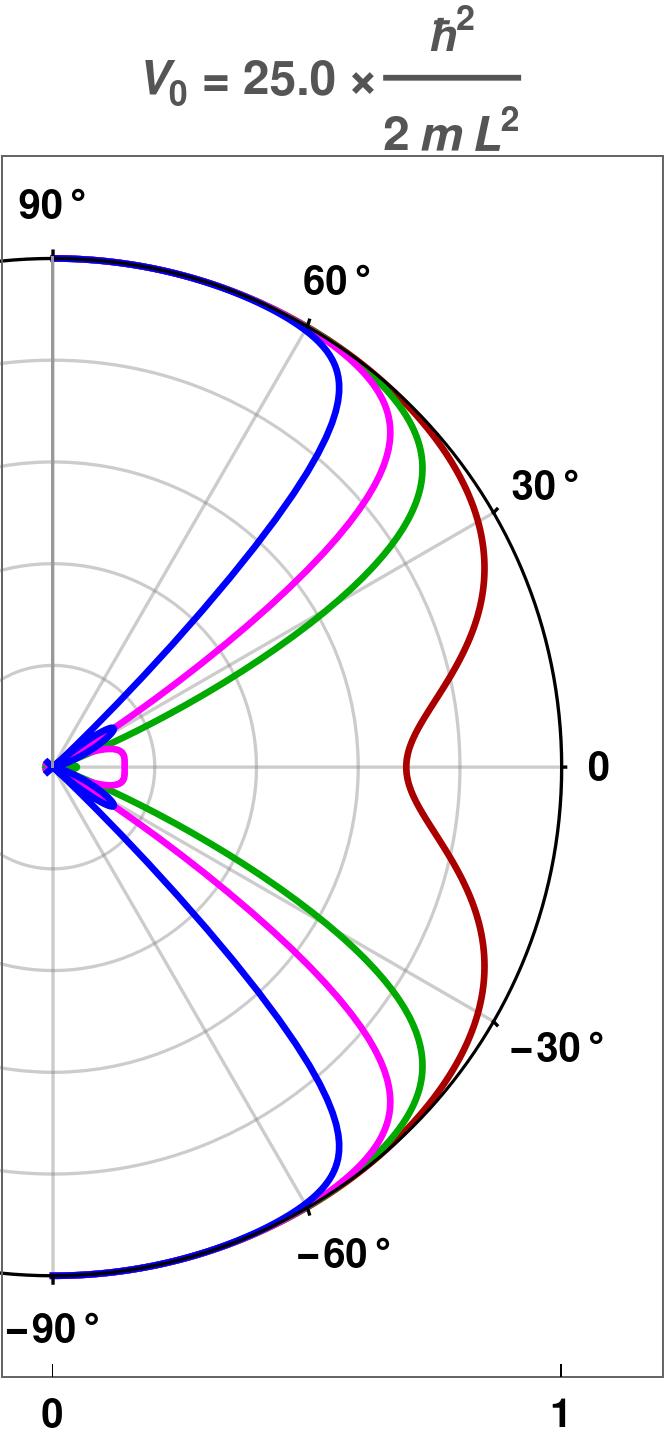
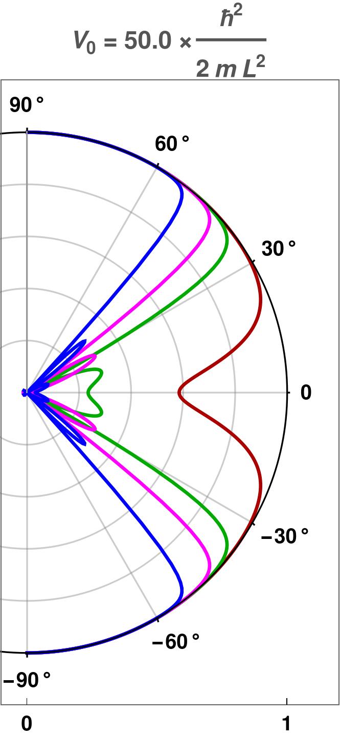
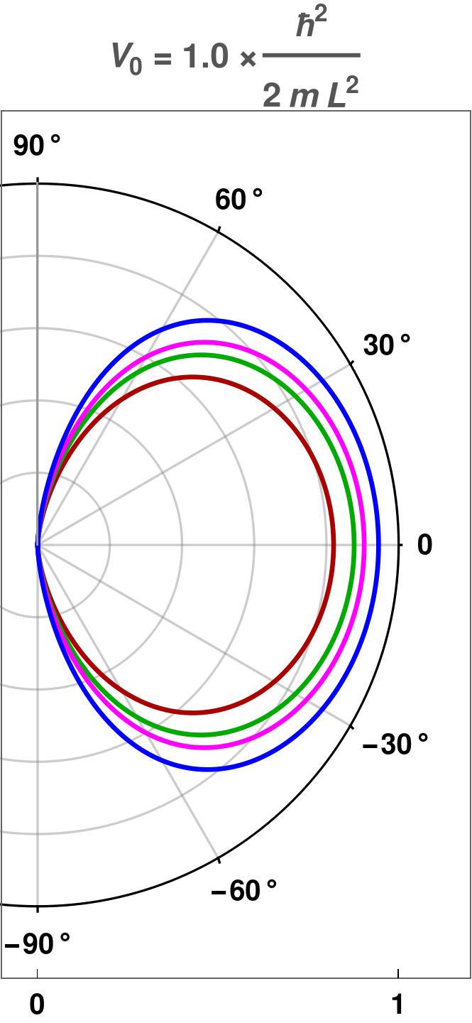
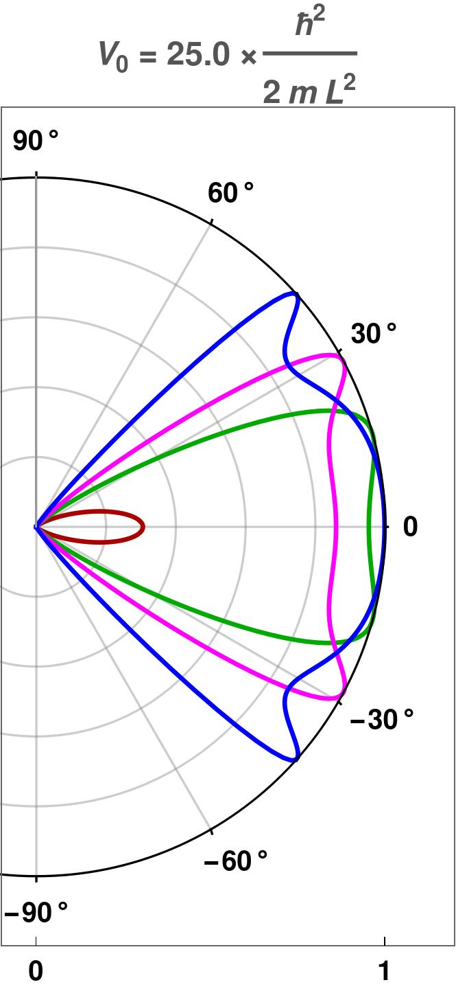
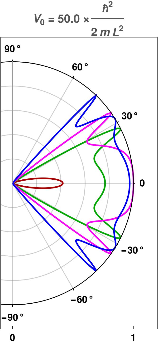
Figure 3: 2d QBCP: The polar plots show the reflection coefficient $R(E,V_{0},\phi)\big{|}_{E>V_{0}}$ and the transmission coefficient $T(E,V_{0},\phi)\big{|}_{E>V_{0}}$ as functions of the incident angle $\phi$ for the parameters $E=1.1\,V_{0}$ (red), $E=1.5\,V_{0}$ (green), $E=1.8\,V_{0}$ (magenta) and $E=2.5\,V_{0}$ (blue).

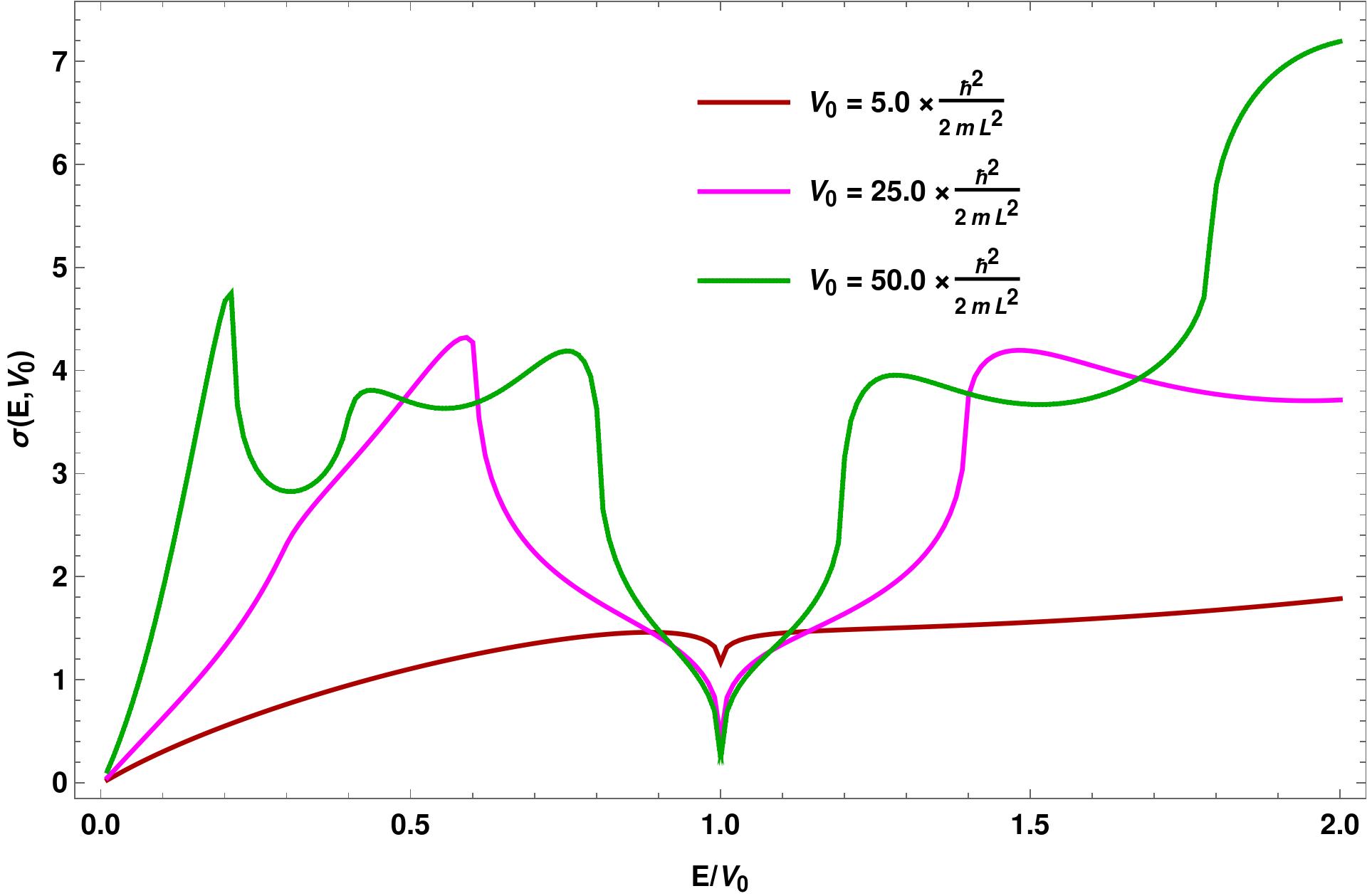
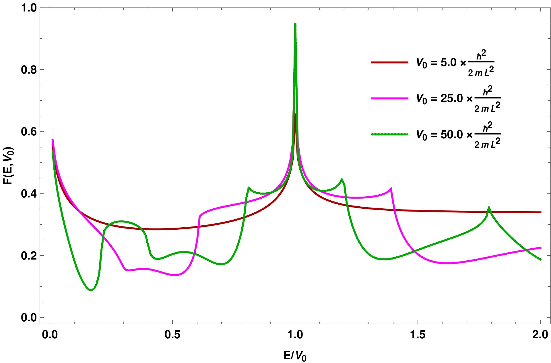
Figure 4: 2d QBCP: Plots of the (a) conductivity ($\sigma$ in units of $2\pi$), and (b) Fano factor ($F$), as functions of $E/V_{0}$, for various values of $V_{0}$.

II.2 Transmission coefficient, conductivity and Fano factor

Let us assume $W$ to be very large such that $q_{n}$ can effectively be treated as a continuous variable. We then numerically compute $T(E,\phi)$.

Using $k_{\ell}=\sqrt{\frac{2mE}{\hbar^{2}}}\cos\phi\,,\quad n=\frac{W\sqrt{2mE}}{h}\sin\phi\,,\quad dn=\frac{2\,W\sqrt{2mE}}{h}\cos\phi\,d\phi$, in the zero-temperature limit and for a small applied voltage, the conductance is given by [15]:

$$G(E,V_{0}) =\frac{e^{2}}{h}\sum_{n}|t_{n}|^{2}\rightarrow\frac{e^{2}}{h}\int|t_{n}(E)|^{2}\,dn=\frac{e^{2}\,W\sqrt{2\,m\,E}}{h^{2}}\int_{-\frac{\pi}{2}}^{\frac{\pi}{2}}T(E,V_{0},\phi)\cos\phi\,d\phi\,.$$ (13)

Therefore, the conductivity is given by:

$$\sigma(E,V_{0}) =\frac{L}{W}\frac{G(E,V_{0})}{e^{2}/h}=2\,\pi\sqrt{\frac{E}{\hbar^{2}/\left(2\,mL^{2}\right)}}\int_{-\frac{\pi}{2}}^{\frac{\pi}{2}}T(E,V_{0},\phi)\cos\phi\,d\phi\,.$$ (14)

Shot noise is the measure of the fluctuations of the current away from their average value. The zero-temperature shot noise is given by [15]:

$$\mathcal{S}(E,V_{0}) =\frac{2\,e^{2}\,\Phi}{h}\sum_{n}|t_{n}|^{2}\,|r_{n}|^{2}\rightarrow\frac{e^{3}\,\Phi\,W\sqrt{\frac{E}{\hbar^{2}/\left(2\,mL^{2}\right)}}}{\pi\,h\,L}\int_{-\frac{\pi}{2}}^{\frac{\pi}{2}}T(E,V_{0},\phi)\left[1-T(E,V_{0},\phi)\right]\,d\phi\,,$$ (15)

where $\Phi$ is the applied voltage, and is characterized by the Fano factor:

$$F(E,V_{0})=\frac{\int_{-\frac{\pi}{2}}^{\frac{\pi}{2}}T(E,V_{0},\phi)\left[1-T(E,V_{0},\phi)\right]\,d\phi}{\int_{-\frac{\pi}{2}}^{\frac{\pi}{2}}T(E,V_{0},\phi)\,d\phi}\,.$$ (16)

We express $E$ and $V_{0}$ in units of $\frac{\hbar^{2}}{2\,mL^{2}}$, and study the behaviour of $T(E,V_{0},\phi)$, $\sigma(E,V_{0})$ and $F(E,V_{0})$. Figs. 2 and 3 show the polar plots of $R(E,V_{0},\phi)$ and $T(E,V_{0},\phi)$ as functions of the incident angle $\phi$, for the cases $E\leq V_{0}$ and $E>V_{0}$ respectively. They also serve to demonstrate that $R(E,V_{0},\phi)+T(E,V_{0},\phi)=1$. From the expression of transmission coefficient in Eq. (34), it is clear that the transmission is zero at normal incidence $(\phi=0)$, as long as $E<V_{0}$. Hence, we do not have a Klein tunneling analogue in the 2d QBCP, unlike graphene [16] or three-band pseudospin-1 Dirac-Weyl systems [17, 18]. However, we still have the resonance conditions $\tilde{k}\,L=\pi N,\,N\in\mathbb{Z}$, under which the barrier becomes transparent $(T=1)$. In Fig. 4, we illustrate the conductivity $\sigma(E,V_{0})$ and the Fano factor $F(E,V_{0})$, as functions of $E/V_{0}$, for some values of $V_{0}$.

III 3d Model

We consider a model for 3d QBCP semimetals, where the low energy bands form a four-dimensional representation of the lattice symmetry group [6]. Then the standard $\left(\mathbf{k}\cdot\mathbf{p}\right)$ Hamiltonian for the particle-hole symmetric system can be written by using the five $4\times 4$ Euclidean Dirac matrices $\Gamma_{a}$ as [12, 19]:

$$\mathcal{H}_{3d}^{kin}(k_{x},k_{y},k_{z})=\frac{\hbar^{2}}{2\,m}\sum_{a=1}^{5}d_{a}(\mathbf{k})\,\,\Gamma_{a}\,.$$ (17)

The $\Gamma_{a}$’s form one of the (two possible) irreducible, four-dimensional Hermitian representations of the five-component Clifford algebra defined by the anticommutator $\{\,\Gamma_{a},\,\Gamma_{b}\}=2\,\delta_{ab}$. The five anticommuting gamma-matrices can always be chosen such that three are real and two are imaginary [12, 20]. In the representation used here, $(\Gamma_{1},\Gamma_{3},\Gamma_{5})$ are real and $(\Gamma_{2},\Gamma_{4})$ are imaginary:

$$\Gamma_{1}=\sigma_{1}\otimes\sigma_{0}\,,\quad\Gamma_{2}=\sigma_{2}\otimes\sigma_{0}\,,\quad\Gamma_{3}=\sigma_{3}\otimes\sigma_{1}\,,\quad\Gamma_{4}=\sigma_{3}\otimes\sigma_{2}\,,\quad\Gamma_{5}=\sigma_{3}\otimes\sigma_{3}\,.$$ (18)

The five functions $d_{a}(\mathbf{k})$ are the real $\ell=2$ spherical harmonics, with the following structure:

$$d_{1}(\mathbf{k})=\sqrt{3}\,k_{y}\,k_{z}\,,\,\,d_{2}(\mathbf{k})=\sqrt{3}\,k_{x}\,k_{z}\,,\,\,d_{3}(\mathbf{k})=\sqrt{3}\,k_{x}\,k_{y},$$

$$d_{4}(\mathbf{k})=\frac{\sqrt{3}}{2}(k_{x}^{2}-k_{y}^{2})\,,\,\,d_{5}(\mathbf{k})=\frac{1}{2}\left(2\,k_{z}^{2}-k_{x}^{2}-k_{y}^{2}\right).$$ (19)

The energy eigenvalues are

$$\varepsilon_{3d}^{\pm}(k_{x},k_{y},k_{z})=\pm\frac{\hbar^{2}\left(k_{x}^{2}+k_{y}^{2}+k_{z}^{2}\right)}{2\,m},$$ (20)

where the “$+$” and “$-$” signs, as usual, refer to the conduction and valence bands. Each of these bands is doubly degenerate.

A set of orthogonal eigenvectors is given by:

$$\Psi_{+,1}^{T} =\frac{1}{\mathcal{N}_{+,1}}\left\{-\frac{(k_{x}+\mathrm{i}\,k_{y})\left(k+k_{z}\right)}{(k_{x}-\mathrm{i}\,k_{y})^{2}},\frac{\mathrm{i}\,\left(k+3\,k_{z}\right)}{\sqrt{3}\,(k_{x}-\mathrm{i}\,k_{y})},-\frac{\mathrm{i}\,\left(-2\,k_{z}\left(k+k_{z}\right)+k_{x}^{2}+k_{y}^{2}\right)}{\sqrt{3}\,(k_{x}-\mathrm{i}\,k_{y})^{2}},1\right\}\,,$$

$$\Psi_{+,2}^{T} =\frac{1}{\mathcal{N}_{+,2}}\left\{\frac{(k_{x}+\mathrm{i}\,k_{y})\left(k-k_{z}\right)}{(k_{x}-\mathrm{i}\,k_{y})^{2}},-\frac{\mathrm{i}\,\left(k-3\,k_{z}\right)}{\sqrt{3}\,(k_{x}-\mathrm{i}\,k_{y})},-\frac{\mathrm{i}\,\left(2\,k_{z}\left(k-k_{z}\right)+k_{x}^{2}+k_{y}^{2}\right)}{\sqrt{3}\,(k_{x}-\mathrm{i}\,k_{y})^{2}},1\right\}\,,$$

$$\Psi_{-,1}^{T} =\frac{1}{\mathcal{N}_{-,1}}\left\{-\frac{\mathrm{i}\,\left(k+k_{z}\right)}{\sqrt{3}\,(k_{x}-\mathrm{i}\,k_{y})},\frac{k-k_{z}}{k_{x}+\mathrm{i}\,k_{y}},1,-\frac{\mathrm{i}\,\left(2\,k_{z}\left(k_{z}-k\right)+k_{x}^{2}+k_{y}^{2}\right)}{\sqrt{3}\,(k_{x}+\mathrm{i}\,k_{y})^{2}}\right\}\,,$$

$$\Psi_{-,2}^{T} =\frac{1}{\mathcal{N}_{-,2}}\left\{\frac{\mathrm{i}\,\left(k-k_{z}\right)}{\sqrt{3}\,(k_{x}-\mathrm{i}\,k_{y})},-\frac{k+k_{z}}{k_{x}+\mathrm{i}\,k_{y}},1,-\frac{\mathrm{i}\,\left(2\,k_{z}\left(k+k_{z}\right)+k_{x}^{2}+k_{y}^{2}\right)}{\sqrt{3}\,(k_{x}+\mathrm{i}\,k_{y})^{2}}\right\}\,,$$ (21)

where $k=\sqrt{k_{x}^{2}+k_{y}^{2}+k_{z}^{2}}$, and the “$+$” (“$-$”) indicates an eigenvector corresponding to the positive (negative) eigenvalue. The symbols $\frac{1}{\mathcal{N}_{\pm,1}}$ and $\frac{1}{\mathcal{N}_{\pm,2}}$ denote the corresponding normalization factors.

The 3d system is modulated by a square electric potential barrier of height $V_{0}$ and width $L$, as described in Eq. (4). Here, we need to consider the total Hamiltonian:

$$\mathcal{H}_{3d}^{tot} =\mathcal{H}_{3d}^{kin}(-\mathrm{i}\,\partial_{x},-\mathrm{i}\,\partial_{y},-\mathrm{i}\,\partial_{z})+V(x)$$ (22)

in position space. As before, we choose the $x$-axis along the transport direction, and place the chemical potential at an energy $E>0$ in the region outside the potential barrier.

III.1 Formalism

We consider the tunneling in a slab of height and width $W$. Again, we assume that the material has a sufficiently large width $W$ along each of the two transverse directions, such that the boundary conditions are irrelevant for the bulk response, and impose the periodic boundary conditions:

$$\tilde{\Psi}^{\mathrm{tot}}(x,0,z)=\tilde{\Psi}^{\mathrm{tot}}(x,W,z)\,,\quad\tilde{\Psi}^{\mathrm{tot}}(x,y,0)=\tilde{\Psi}^{\mathrm{tot}}(x,y,W)\,.$$ (23)

The transverse momentum $\mathbf{k}_{\perp}=(k_{y},k_{z})$ is conserved, and its components are quantized. Due to periodicity, we conclude that:

$$k_{y}=\frac{2\,\pi\,n_{y}}{W}\equiv q_{n_{y}}\,,\quad k_{z}=\frac{2\,\pi\,n_{z}}{W}\equiv q_{n_{z}}\,,$$ (24)

where $(n_{x},n_{y})\in\mathbb{Z}$. For the longitudinal direction (along the $x$-axis), we seek plane wave solutions of the form $e^{\mathrm{i}\,k_{x}x}$. Then the full wavefunction is given by:

$$\tilde{\Psi}^{\mathrm{tot}}(x,y,z,\mathbf{n})=\text{const.}\times\tilde{\Psi}_{\mathbf{n}}(x)\,e^{\mathrm{i}\left(q_{n_{y}}y+q_{n_{z}}z\right)}\text{ with }\mathbf{n}=(n_{y},n_{z})\,.$$ (25)

For any mode of given transverse momentum component $\mathbf{k}_{\perp}$, we can determine the $x$-component of the wavevectors of the incoming, reflected, and transmitted waves (denoted by $k_{\ell}$), by solving $\varepsilon_{3d}^{\pm}(k_{x},\mathbf{n})=\pm\frac{\hbar^{2}\left(k_{\ell}^{2}+{\mathbf{k}_{\perp}}^{2}\right)}{2\,m}\,.$ In the regions $x<0$ and $x>L$, we have only propagating modes ($k_{\ell}$ is real), while the $x$-components in the scattering region (denoted by $\tilde{k}$), are given by $\tilde{k}^{2}=\frac{2\,m\,|E-V_{0}|}{\hbar^{2}}-{\mathbf{k}_{\perp}}^{2}$, and may be propagating ($\tilde{k}$ is real) or evanescent ($\tilde{k}$ is imaginary).

We will follow the same procedure as described for the 2d QBCP. Again, without any loss of generality, we consider the transport of one of the degenerate positive energy states ($\Psi_{+,1}$) corresponding to electron-like particles, with the Fermi level outside the potential barrier being adjusted to a value $E=\varepsilon_{3d}^{+}(k_{x},k_{y},k_{z})$. In this case, a scattering state $\tilde{\Psi}_{\mathbf{n}}$, in the mode labeled by $\mathbf{n}$, is constructed from the states:

$$\tilde{\Psi}_{\mathbf{n}}(x)= \begin{cases}\tilde{\phi}_{L}&\text{ for }x<0\,,\\ \tilde{\phi}_{M}&\text{ for }0<x<L\,,\\ \tilde{\phi}_{R}&\text{ for }x>L\,,\end{cases}$$

$$\tilde{\phi}_{L}= \,\frac{\Psi_{+,1}(k_{\ell},q_{n_{y}},q_{n_{z}})\,e^{\mathrm{i}\,k_{\ell}x}+\sum\limits_{s=1,2}r_{\mathbf{n},s}\,\Psi_{+,s}(-k_{\ell},q_{n_{y}},q_{n_{z}})\,e^{-\mathrm{i}\,k_{\ell}x}}{\sqrt{\tilde{\mathcal{V}}(k_{\ell},\mathbf{n})}}\,,$$

$$\tilde{\phi}_{M}= \,\Big{[}\sum\limits_{s=1,2}\alpha_{\mathbf{n},s}\,\Psi_{+,s}(\tilde{k},q_{n_{y}},q_{n_{z}})\,e^{\mathrm{i}\,\tilde{k}\,x}+\sum\limits_{s=1,2}\beta_{\mathbf{n},s}\,\Psi_{+,s}(-\tilde{k},q_{n_{y}},q_{n_{z}})\,e^{-\mathrm{i}\,\tilde{k}\,x}\Big{]}\Theta\left(E-V_{0}\right)$$

$$+\Big{[}\sum\limits_{s=1,2}\alpha_{\mathbf{n},s}\,\Psi_{-,s}(\tilde{k},q_{n_{y}},q_{n_{z}})\,e^{\mathrm{i}\,\tilde{k}\,x}+\sum\limits_{s=1,2}\beta_{\mathbf{n},s}\,\Psi_{-,s}(-\tilde{k},q_{n_{y}},q_{n_{z}})\,e^{-\mathrm{i}\,\tilde{k}\,x}\Big{]}\,\Theta\left(V_{0}-E\right)\,,$$

$$\tilde{\phi}_{R}= \,\frac{\sum\limits_{s=1,2}t_{\mathbf{n},s}\,\Psi_{+,s}(k_{\ell},q_{n_{y}},q_{n_{z}})}{\sqrt{\tilde{\mathcal{V}}(k_{\ell},\mathbf{n})}}\,e^{\mathrm{i}\,k_{\ell}\left(x-L\right)},$$

$$\tilde{\mathcal{V}}(k_{\ell},\mathbf{n})\equiv \,|\partial_{k_{\ell}}\varepsilon_{3d}^{+}(k_{\ell},\mathbf{n})|=\frac{\hbar^{2}k_{\ell}}{m}\,,\quad k_{\ell}=\sqrt{\frac{2\,m\,E}{\hbar^{2}}-q_{n_{y}}^{2}-q_{n_{z}}^{2}}\,,\quad\tilde{k}=\sqrt{\frac{2\,m\,|E-V_{0}|}{\hbar^{2}}-q_{n_{y}}^{2}-q_{n_{z}}^{2}}\,,$$ (26)

where we have used the velocity $\tilde{\mathcal{V}}(k_{\ell},\mathbf{n})$ to normalize the incident, reflected and transmitted plane waves. Note that for $V_{0}>E$, the Fermi level within the potential barrier lies within the valence band, and we must use the valence band wavefunctions in that regio

The usual mode-matching procedure at $x=0$ and $x=L$ gives us :

$$r_{\mathbf{n},1}(E,V_{0}) =\begin{cases}\frac{\sin\left({\tilde{k}}L\right)\left(\mathrm{i}\,k_{y}+k_{\ell}\right)\left[k_{\ell}\,k_{z}+\mathrm{i}\,k_{y}\sqrt{k_{\ell}^{2}+k_{y}^{2}+k_{z}^{2}}\right)\left({\tilde{k}}^{2}\left(8k_{\ell}^{2}-k_{y}^{2}-k_{z}^{2}\right)+\left(k_{y}^{2}+k_{z}^{2}\right)\left(5k_{\ell}^{2}-4\left(k_{y}^{2}+k_{z}^{2}\right)\right)\right]}{2\left(k_{\ell}-\mathrm{i}\,k_{y}\right)^{2}\sqrt{k_{\ell}^{2}+k_{y}^{2}+k_{z}^{2}}\,\left[\sin\left({\tilde{k}}L\right)\left\{{\tilde{k}}^{2}\left(4k_{\ell}^{2}+k_{y}^{2}+k_{z}^{2}\right)+\left(k_{y}^{2}+k_{z}^{2}\right)\left(k_{\ell}^{2}+4\left(k_{y}^{2}+k_{z}^{2}\right)\right)\right\}-6\,\mathrm{i}\,{\tilde{k}}k_{\ell}\cos\left({\tilde{k}}L\right)\left(k_{y}^{2}+k_{z}^{2}\right)\right]}&\text{ for }E<V_{0}\\ \frac{\left(k_{\ell}^{2}-{\tilde{k}}^{2}\right)\sin\left({\tilde{k}}L\right)(k_{\ell}+\mathrm{i}\,k_{y})\left(k_{\ell}k_{z}+\mathrm{i}\,k_{y}\sqrt{k_{\ell}^{2}+k_{y}^{2}+k_{z}^{2}}\right)}{(k_{\ell}-\mathrm{i}\,k_{y})^{2}\sqrt{k_{\ell}^{2}+k_{y}^{2}+k_{z}^{2}}\,\left[\left({\tilde{k}}^{2}+k_{\ell}^{2}\right)\sin\left({\tilde{k}}L\right)+2\,\mathrm{i}\,{\tilde{k}}k_{\ell}\cos\left({\tilde{k}}L\right)\right]}&\text{ for }E>V_{0}\end{cases}\,,$$

$$r_{\mathbf{n},2}(E,V_{0}) =\begin{cases}-\frac{{\tilde{k}}^{2}\left[4k_{\ell}^{2}-5\left(k_{y}^{2}+k_{z}^{2}\right)\right]+\left(k_{y}^{2}+k_{z}^{2}\right)\left[k_{\ell}^{2}-8\left(k_{y}^{2}+k_{z}^{2}\right)\right]\sin\left({\tilde{k}}L\right)}{\sin\left({\tilde{k}}L\right)\left[{\tilde{k}}^{2}\left(4k_{\ell}^{2}+k_{y}^{2}+k_{z}^{2}\right)+\left(k_{y}^{2}+k_{z}^{2}\right)\left\{k_{\ell}^{2}+4\left(k_{y}^{2}+k_{z}^{2}\right)\right\}\right]-6\,\mathrm{i}\,{\tilde{k}}k_{\ell}\cos\left({\tilde{k}}L\right)\left(k_{y}^{2}+k_{z}^{2}\right)}&\\ \times\frac{k_{\ell}\left(k_{\ell}+\mathrm{i}\,k_{y}\right)\left(\sqrt{k_{\ell}^{2}+k_{y}^{2}+k_{z}^{2}}+k_{z}\right)\sqrt{\left(k_{z}\left(k_{z}-\sqrt{k_{\ell}^{2}+k_{y}^{2}+k_{z}^{2}}\right)+k_{\ell}^{2}+k_{y}^{2}\right)}}{\left(k_{\ell}-\mathrm{i}\,k_{y}\right)^{2}\sqrt{k_{\ell}^{2}+k_{y}^{2}+k_{z}^{2}}\,\sqrt{k_{z}\left(\sqrt{k_{\ell}^{2}+k_{y}^{2}+k_{z}^{2}}+k_{z}\right)+k_{\ell}^{2}+k_{y}^{2}}}&\text{ for }E<V_{0}\\ \frac{k_{\ell}\left({\tilde{k}}^{2}-k_{\ell}^{2}\right)\sin\left({\tilde{k}}L\right)(k_{\ell}+\mathrm{i}\,k_{y})\left(\sqrt{k_{\ell}^{2}+k_{y}^{2}+k_{z}^{2}}+k_{z}\right)\sqrt{k_{z}\left(k_{z}-\sqrt{k_{\ell}^{2}+k_{y}^{2}+k_{z}^{2}}\right)+k_{\ell}^{2}+k_{y}^{2}}}{(k_{\ell}-\mathrm{i}\,k_{y})^{2}\sqrt{k_{\ell}^{2}+k_{y}^{2}+k_{z}^{2}}\,\sqrt{k_{z}\left(\sqrt{k_{\ell}^{2}+k_{y}^{2}+k_{z}^{2}}+k_{z}\right)+k_{\ell}^{2}+k_{y}^{2}}\,\left[\left({\tilde{k}}^{2}+k_{\ell}^{2}\right)\sin\left({\tilde{k}}L\right)+2\mathrm{i}\,{\tilde{k}}k_{\ell}\cos\left({\tilde{k}}L\right)\right]}&\text{ for }E>V_{0}\end{cases}\,,$$ (27)

and

$$t_{\mathbf{n},1}(E,V_{0}) =\begin{cases}-\frac{6\,\mathrm{i}\,{\tilde{k}}\,k_{\ell}\left(k_{y}^{2}+k_{z}^{2}\right)}{\sin\left({\tilde{k}}L\right)\left[{\tilde{k}}^{2}\left(4\,k_{\ell}^{2}+k_{y}^{2}+k_{z}^{2}\right)+\left(k_{y}^{2}+k_{z}^{2}\right)\left\{k_{\ell}^{2}+4\left(k_{y}^{2}+k_{z}^{2}\right)\right\}\right]-6\,\mathrm{i}\,{\tilde{k}}\,k_{\ell}\cos\left({\tilde{k}}L\right)\left(k_{y}^{2}+k_{z}^{2}\right)}&\text{ for }E<V_{0}\\ \frac{-2\,\mathrm{i}\,{\tilde{k}}\,k_{\ell}}{\left({\tilde{k}}^{2}+k_{\ell}^{2}\right)\sin\left({\tilde{k}}L\right)+2\,\mathrm{i}\,{\tilde{k}}\,k_{\ell}\cos\left({\tilde{k}}L\right)}&\text{ for }E>V_{0}\end{cases}\,,$$

$$t_{\mathbf{n},2}(E,V_{0}) =0\,.$$ (28)

The reflection and transmission coefficients at an energy $E$ are given by

$$R(E,V_{0},\theta,\phi)=|r_{\mathbf{n},1}(E,V_{0})|^{2}+|r_{\mathbf{n},2}(E,V_{0})|^{2}\text{ and }T(E,V_{0},\theta,\phi)=|t_{\mathbf{n},1}(E,V_{0})|^{2}$$ (29)

respectively, where $\theta=\cos^{-1}\left(\frac{\hbar\,q_{n_{z}}}{\sqrt{2\,m\,E}}\right)$ and $\phi=\tan^{-1}\left(\frac{q_{n_{y}}}{k_{\ell}}\right)$ define the incident angle (solid) of the incoming wave in 3d.

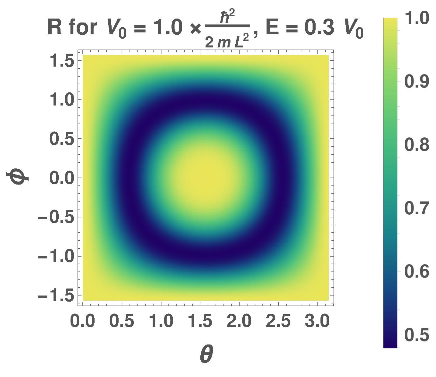
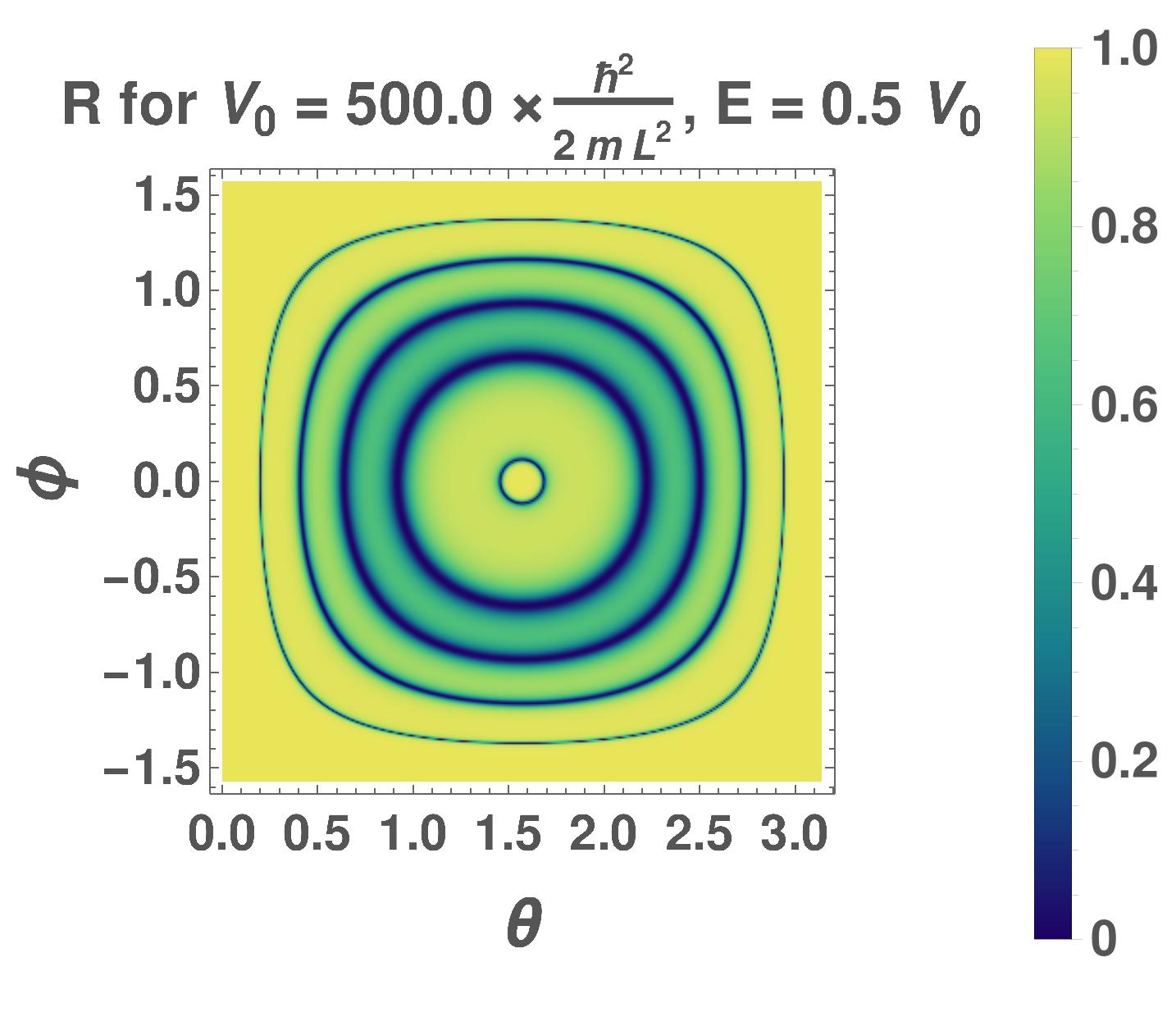
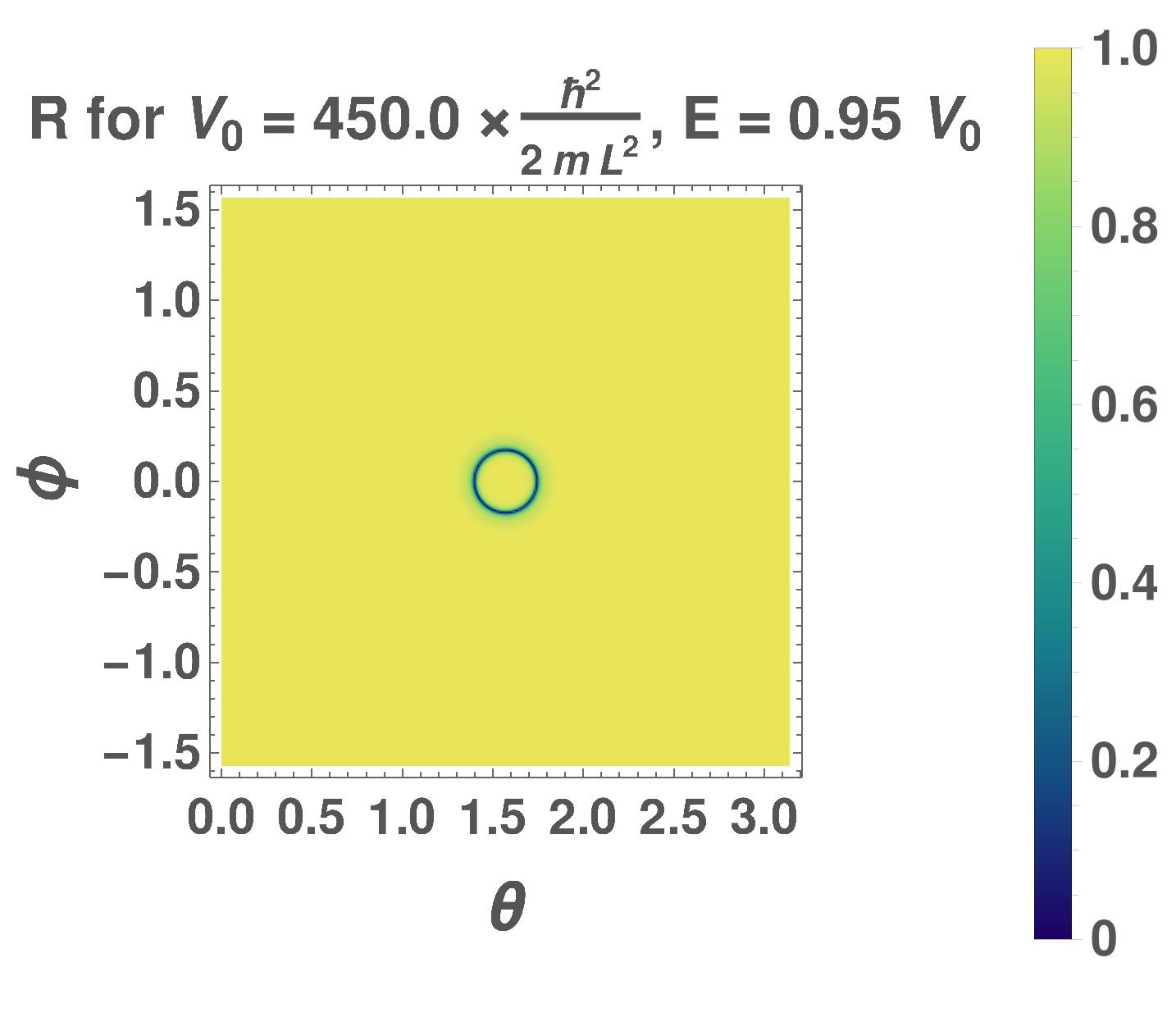
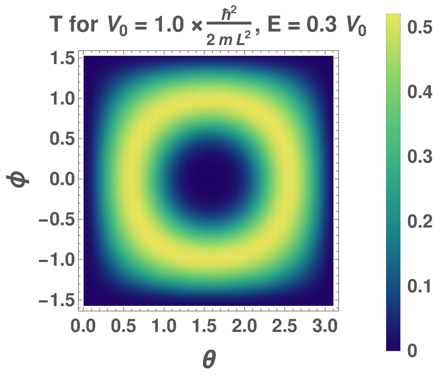
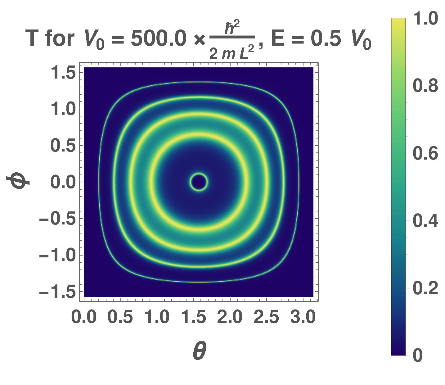
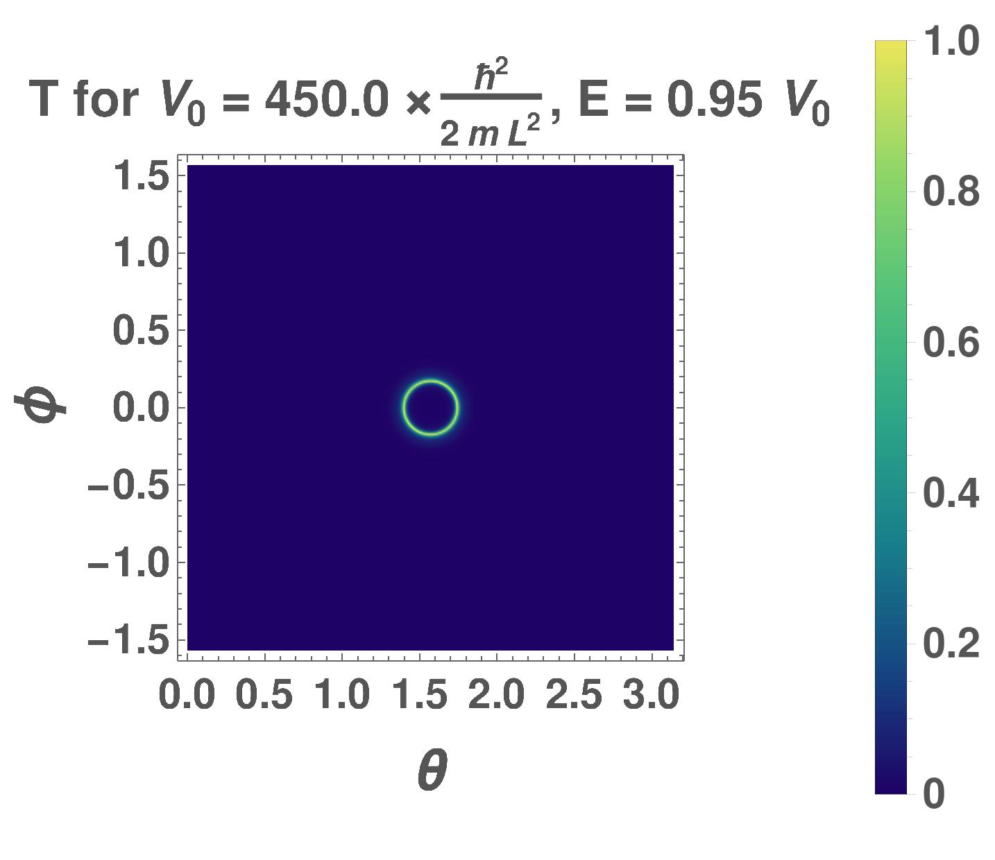
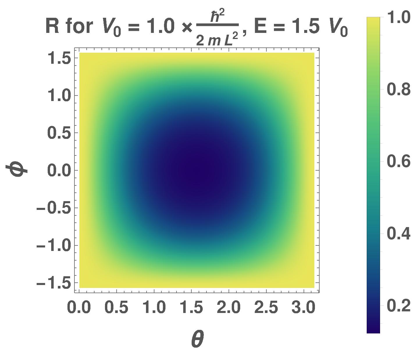
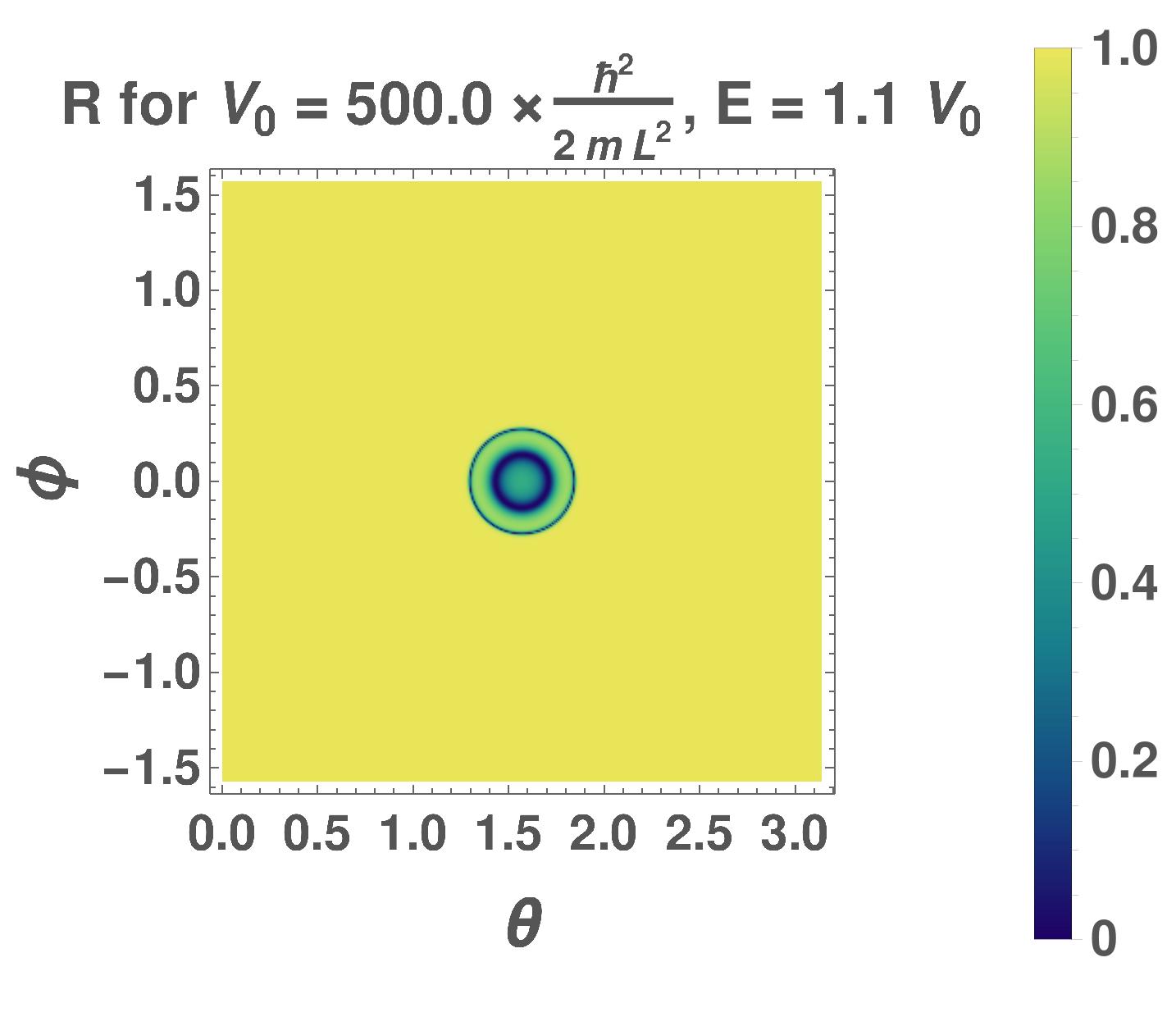
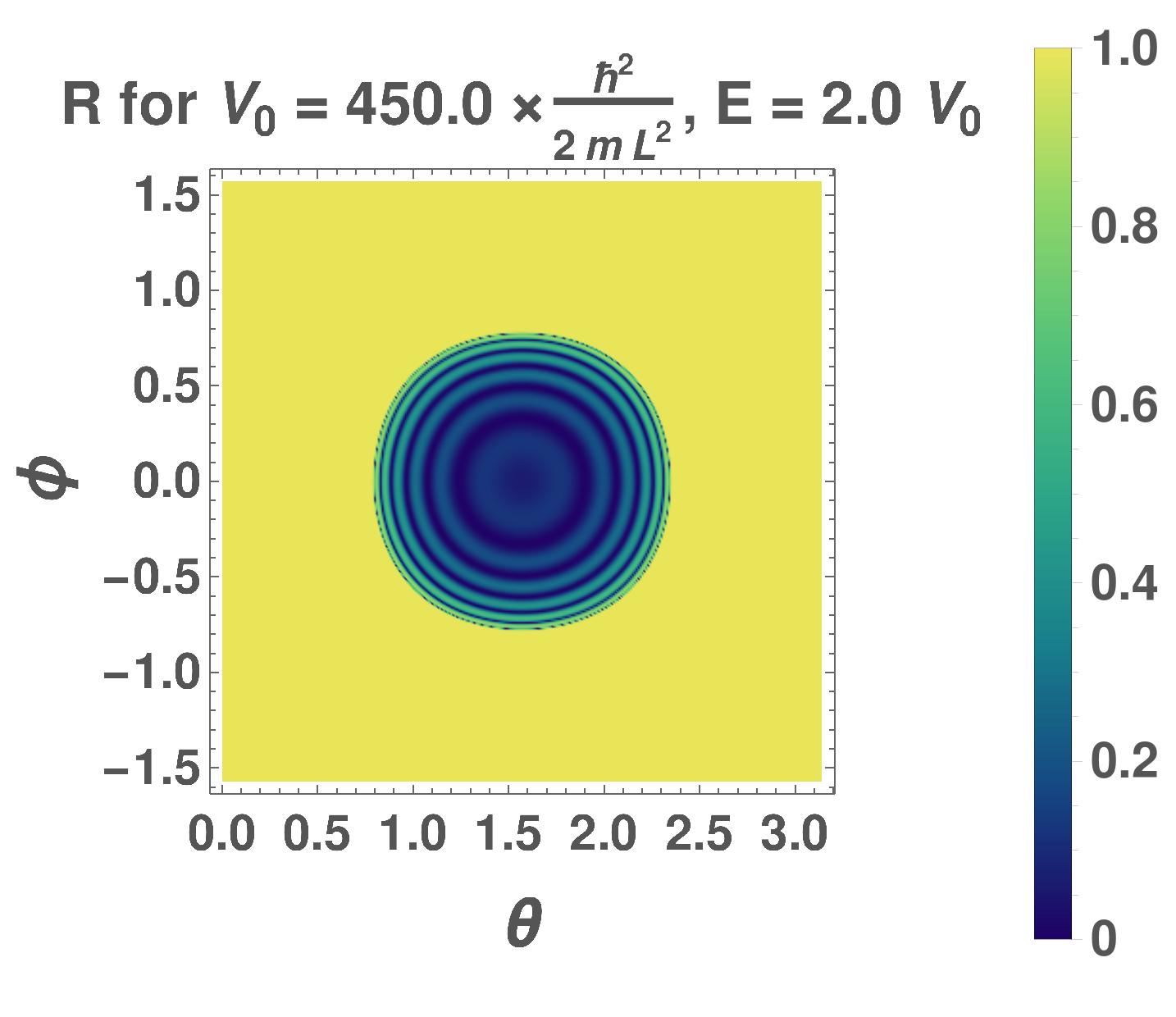
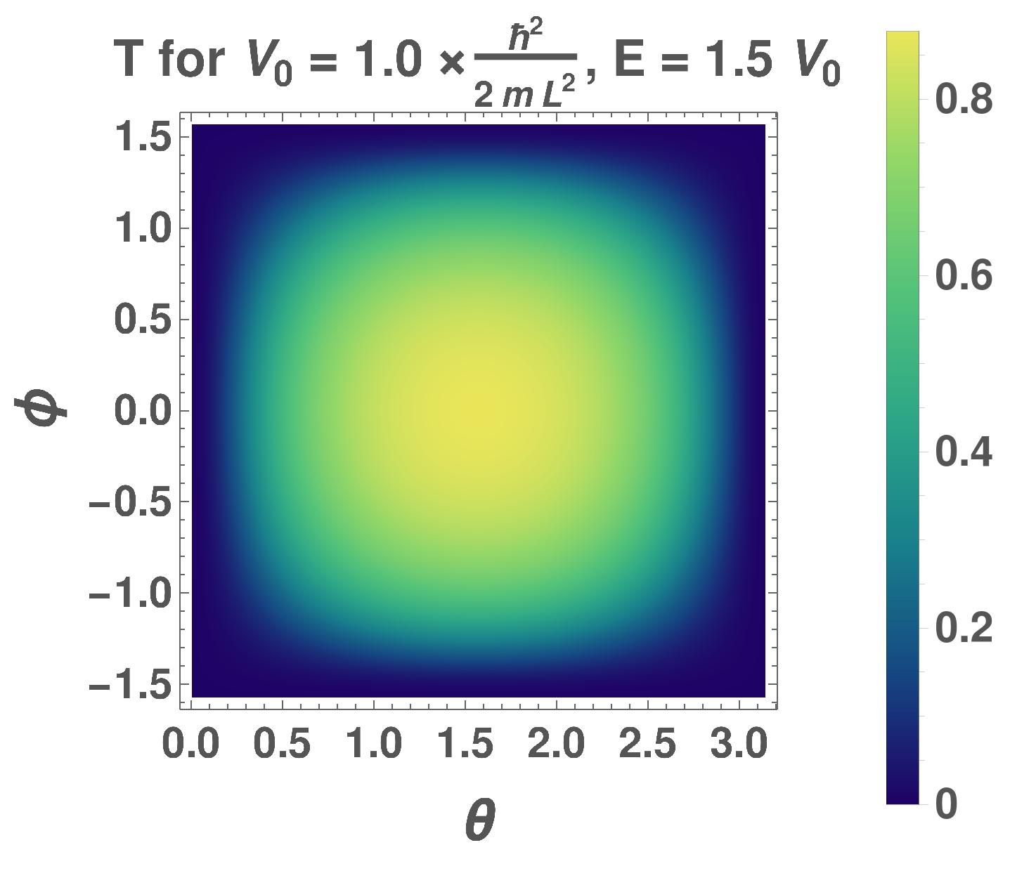
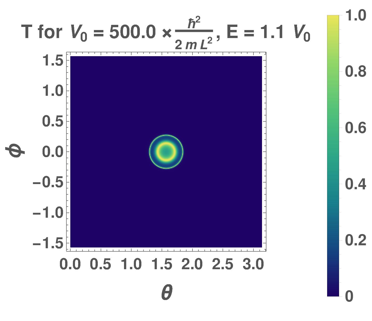
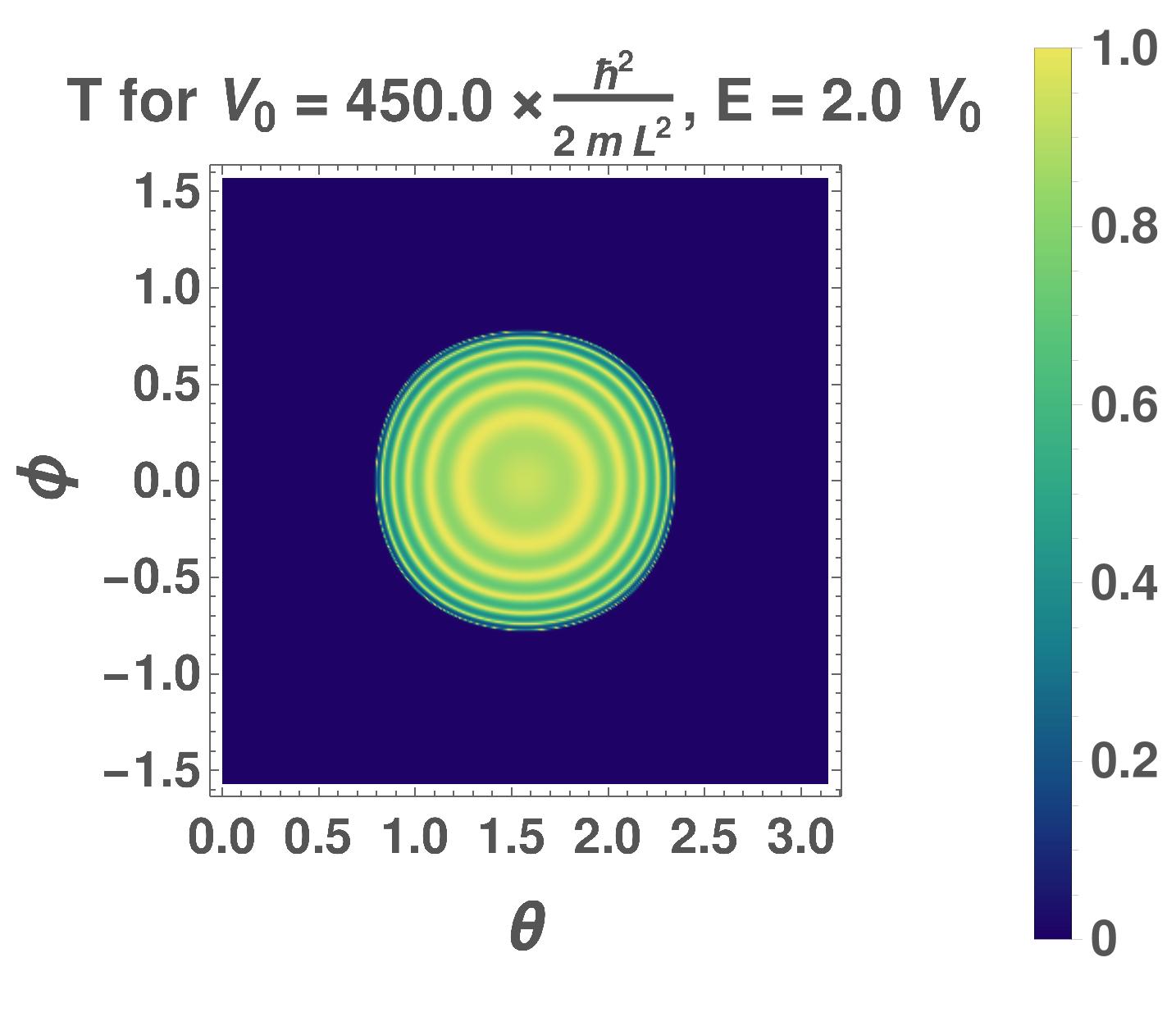
Figure 5: Contourplots of the reflection coefficient ($R$) and transmission coefficient ($T$) for $3d$ QBCP as functions of $(\theta,\phi)$, for various values of $V_{0}$ and $E$.

III.2 Transmission coefficient, conductivity and Fano factor

Again, we assume $W$ to be very large such that $\left(q_{n_{y}},q_{n_{z}}\right)$ can effectively be treated as continuous variables. Using $k_{\ell}=\sqrt{\frac{2mE}{\hbar^{2}}}\sin\theta\cos\phi,$ $n_{y}=\frac{W\sqrt{2mE}}{h}\sin\theta\sin\phi,$ and $n_{z}=\frac{W\sqrt{2mE}}{h}\cos\theta,$ we get $dn_{y}\,dn_{z}=\frac{W^{2}\times 2\,m\,E}{h^{2}}\cos\phi\sin^{2}\theta\,d\phi\,d\theta$. Hence, in the zero-temperature limit, and for a small applied voltage, the conductance is given by [15]:

$$G(E,V_{0}) =\frac{2\,e^{2}}{h}\sum_{\mathbf{n}}|t_{\mathbf{n},1}|^{2}$$

$$\rightarrow\frac{2\,e^{2}}{h}\int|t_{\mathbf{n},1}|^{2}\,dn_{x}\,dn_{y}$$

$$\qquad=\frac{4\,\pi\,e^{2}\,W^{2}}{\hbar}\left(\frac{2\,m\,E}{\hbar^{2}}\right)\int_{\theta=0}^{\pi}\int_{\phi=-\frac{\pi}{2}}^{\frac{\pi}{2}}T(E,V_{0},\theta,\phi)\cos\phi\sin^{2}\theta\,d\phi\,d\theta,$$ (30)

leading to the conductivity expression:

$$\sigma(E,V_{0}) =\left(\frac{L}{W}\right)^{2}\frac{G(E,V_{0})}{e^{2}/h}$$

$$=8\,\pi^{2}\left[\frac{E}{\hbar^{2}/\left(2\,mL^{2}\right)}\right]\int_{\theta=0}^{\pi}\int_{\phi=-\frac{\pi}{2}}^{\frac{\pi}{2}}T(E,V_{0},\theta,\phi)\cos\phi\sin^{2}\theta\,d\phi\,d\theta.$$ (31)

Note that there is a twofold degeneracy because we have two independent conduction band states, and hence an extra factor of two has been included in the expressions for $G$ and $\sigma$.

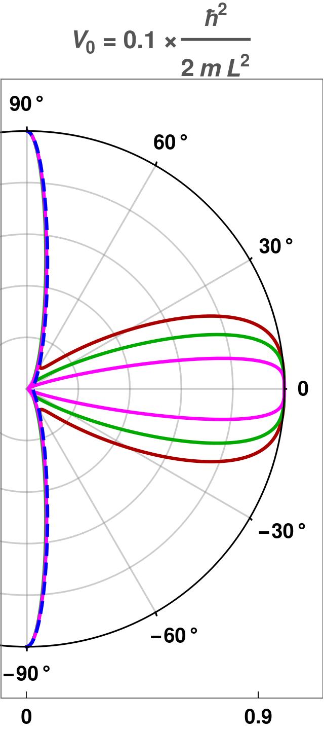
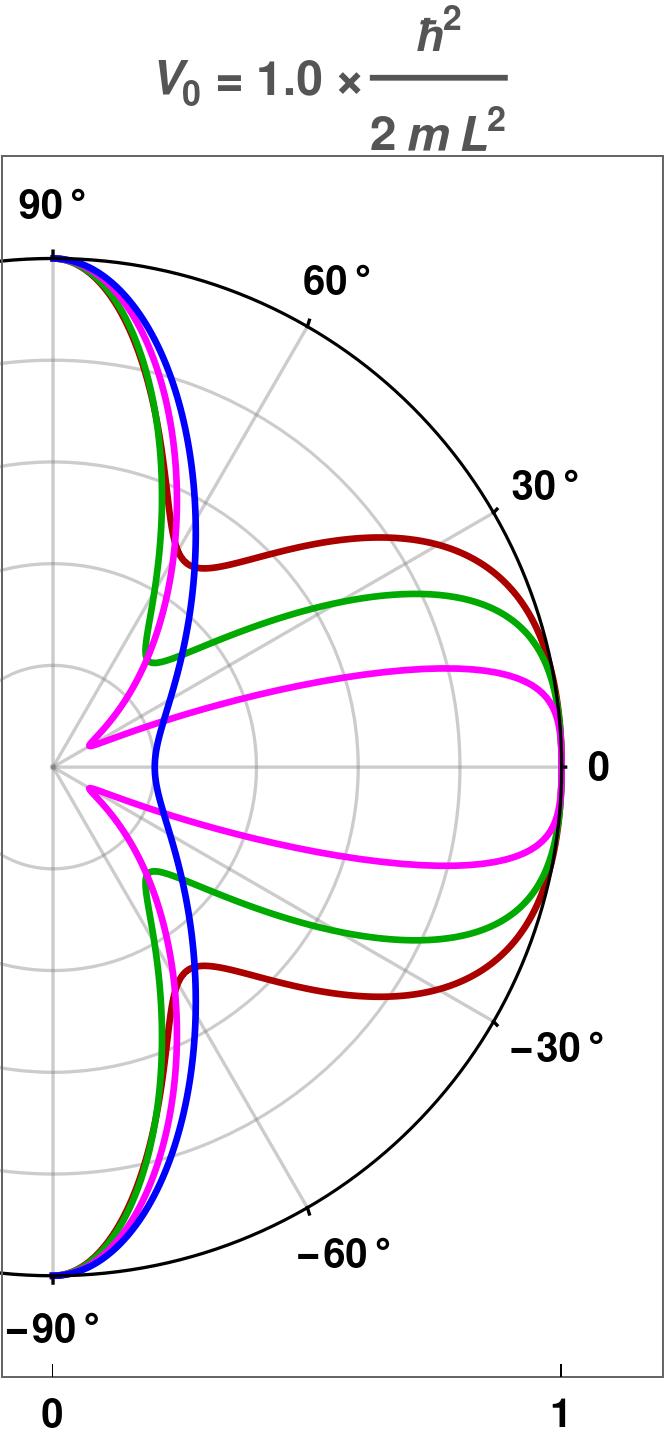
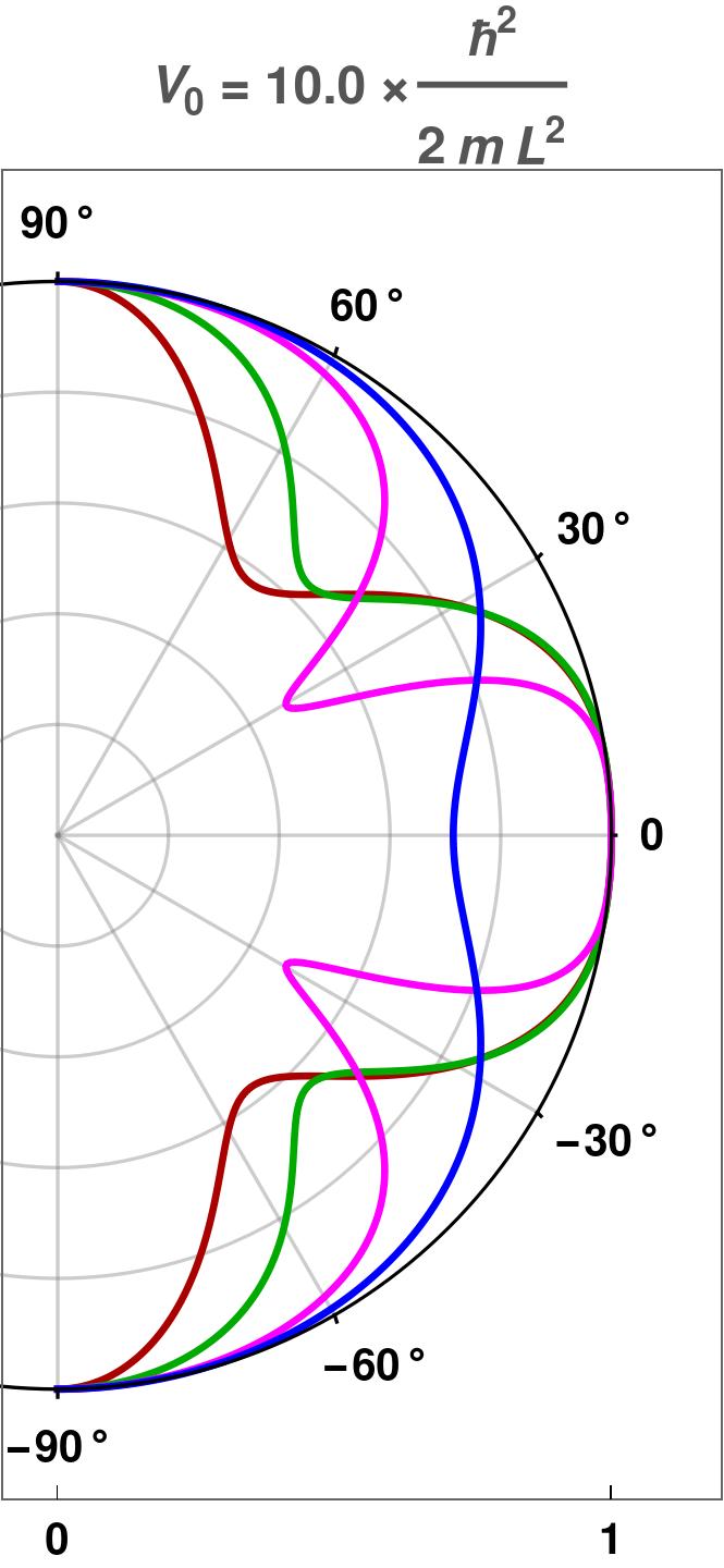
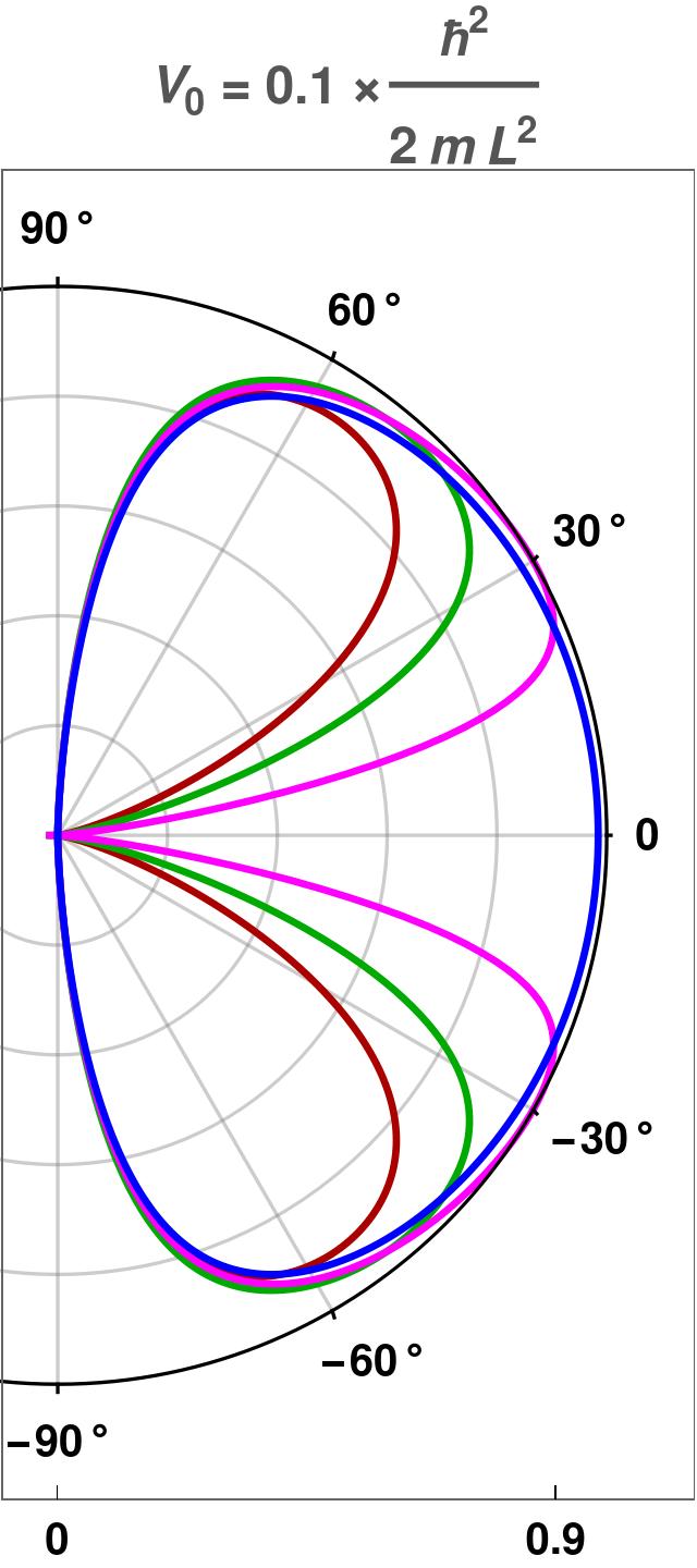
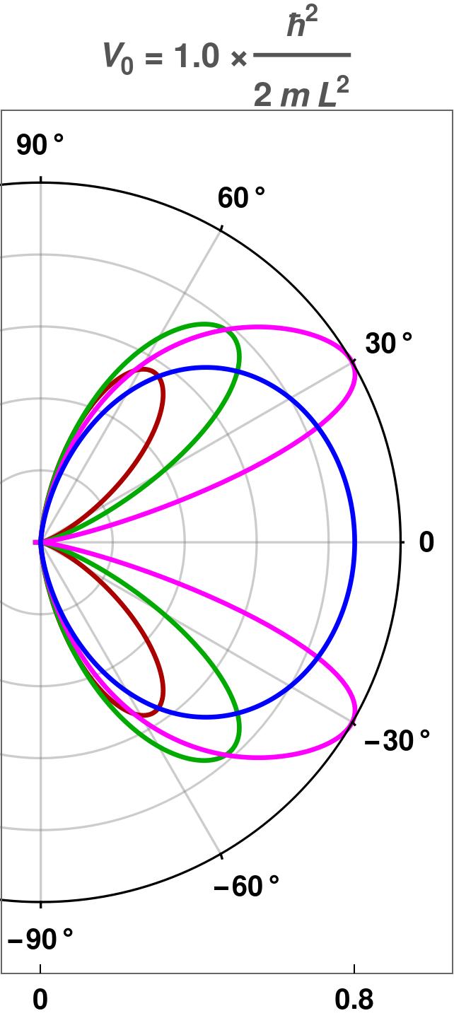
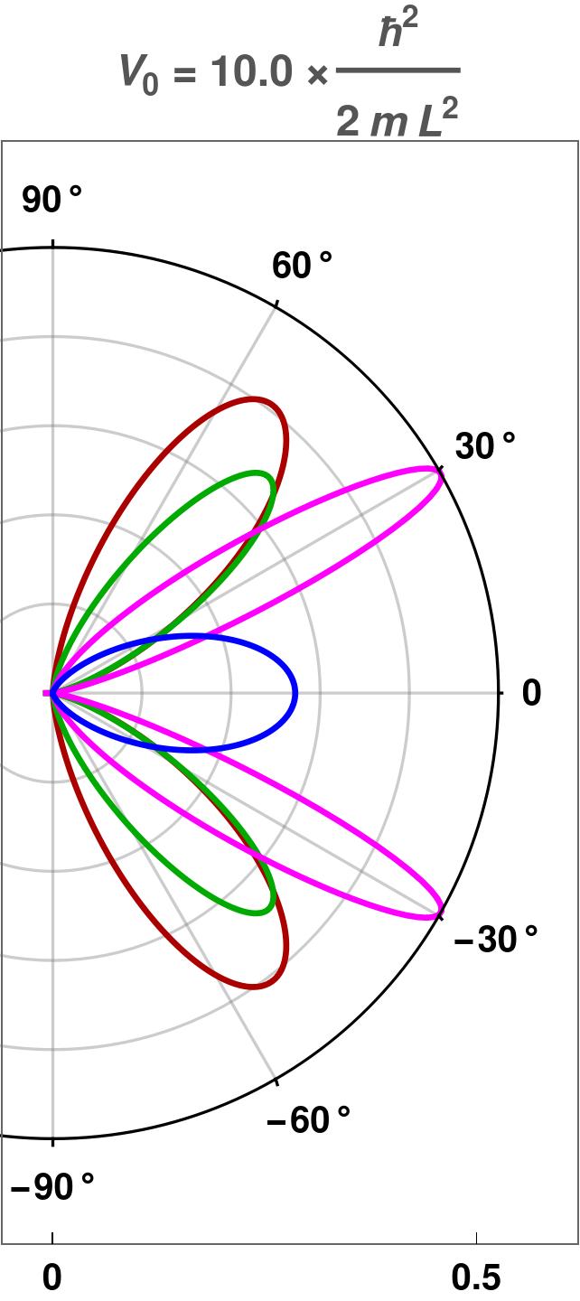
Figure 6: 3d QBCP: The polar plots show the reflection coefficient $R(E,V_{0},\theta,\frac{\pi}{2})\big{|}_{E\leq V_{0}}$ and the transmission coefficient $T(E,V_{0},\theta,\frac{\pi}{2})\big{|}_{E\leq V_{0}}$as functions of the incident angle $\phi$ (in the $xy-$plane with no $k_{z}-$component) for the parameters $E=0.3\,V_{0}$ (red), $E=0.5\,V_{0}$ (green), $E=0.8\,V_{0}$ (magenta) and $E=1.0\,V_{0}$ (blue).

$$\mathcal{S}(E,V_{0}) =\frac{4\,e^{2}\,\Phi}{h}\sum_{\mathbf{n}}|t_{\mathbf{n},1}|^{2}\left(1-|t_{\mathbf{n},1}|^{2}\right)$$

$$\rightarrow\frac{8\,\pi\,e^{3}\,W^{2}\,\Phi}{\hbar}\left(\frac{2\,m\,E}{\hbar^{2}}\right)\int_{\theta=0}^{\pi}\int_{\phi=-\frac{\pi}{2}}^{\frac{\pi}{2}}T(E,V_{0},\theta,\phi)\left[1-T(E,V_{0},\theta,\phi)\right]\,d\phi\,d\theta,$$ (32)

and

$$F(E,V_{0}) =\frac{\int_{\theta=0}^{\pi}\int_{\phi=-\frac{\pi}{2}}^{\frac{\pi}{2}}T(E,V_{0},\theta,\phi)\left[1-T(E,V_{0},\theta,\phi)\right]\cos\phi\sin^{2}\theta\,d\phi\,d\theta}{\int_{\theta=0}^{\pi}\int_{\phi=-\frac{\pi}{2}}^{\frac{\pi}{2}}T(E,V_{0},\theta,\phi)\cos\phi\sin^{2}\theta\,d\phi\,d\theta}\,,$$ (33)

respectively. Here, $\Phi$ is the applied voltage.

As before, we express $E$ and $V_{0}$ in units of $\frac{\hbar^{2}}{2\,mL^{2}}$, and study the behaviour of $T(E,V_{0},\theta,\phi)$, $\sigma(E,V_{0})$ and $F(E,V_{0})$. From the expression of transmission coefficient in Eq. (28), it is clear that the transmission is zero at normal incidence $(\theta=\pi/2,\phi=0)$, as long as $E<V_{0}$. This is analogous to the 2d case. In Fig. 5, we show the angular dependence of $R(E,V_{0},\theta,\phi)$ and $T(E,V_{0},\theta,\phi)$ via contourplots. Fig. 6 shows the polar plots of $R(E,V_{0},\pi/2,\phi)$ and $T(E,V_{0},\pi/2,\phi)$ as functions of the incident angle $\phi$ for $E\leq V_{0}$, which corresponds to $k_{z}=0$. Since the transmission coefficient for $E>V_{0}$ has the same expression both for the 2d and 3d QBCPs, the polar plots of $T(E,V_{0},\pi/2,\phi)\big{|}_{E>V_{0}}$ will be identical to Fig. 3. In Fig. 7, we illustrate the conductivity $\sigma(E,V_{0})$ and the Fano factor $F(E,V_{0})$, as functions of $E/V_{0}$, for some values of $V_{0}$.

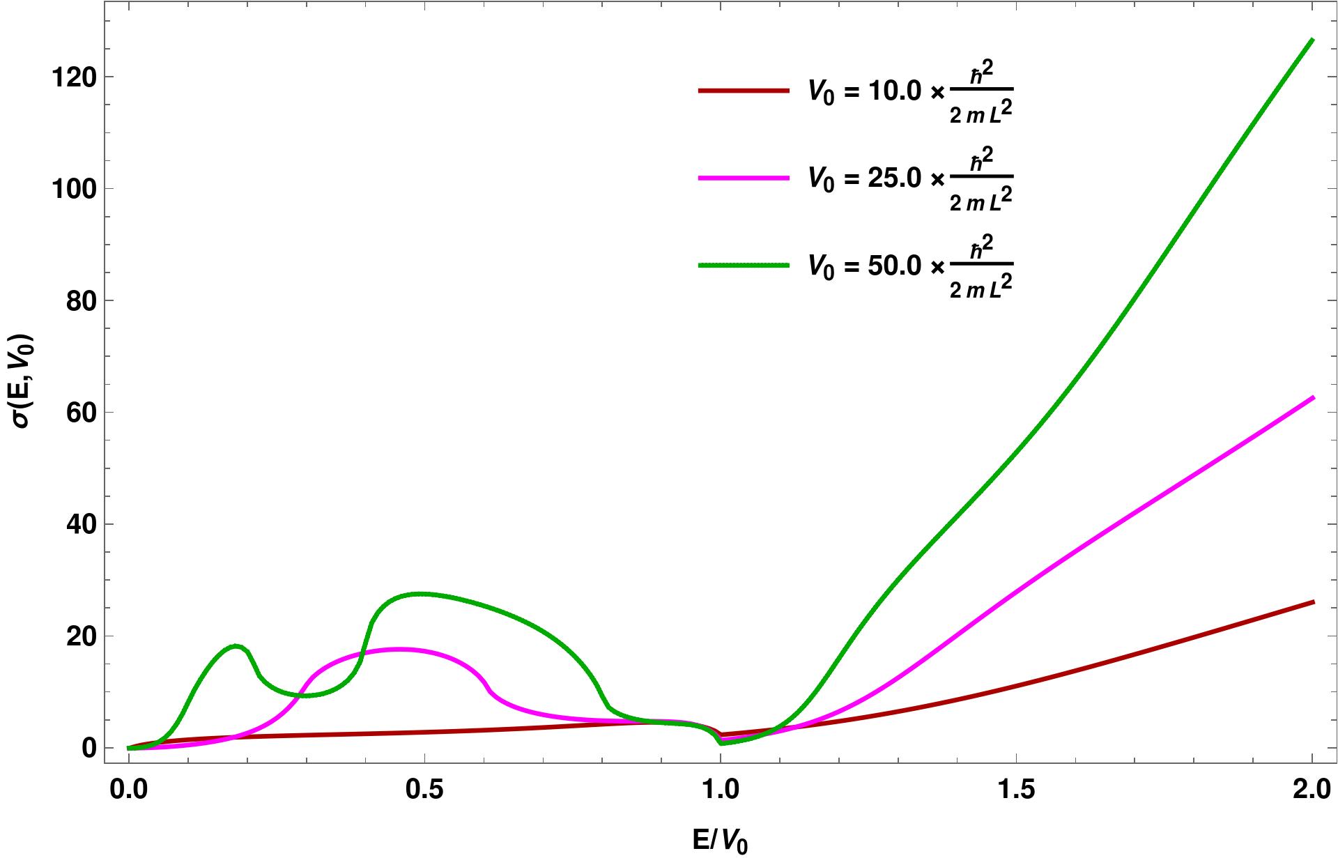
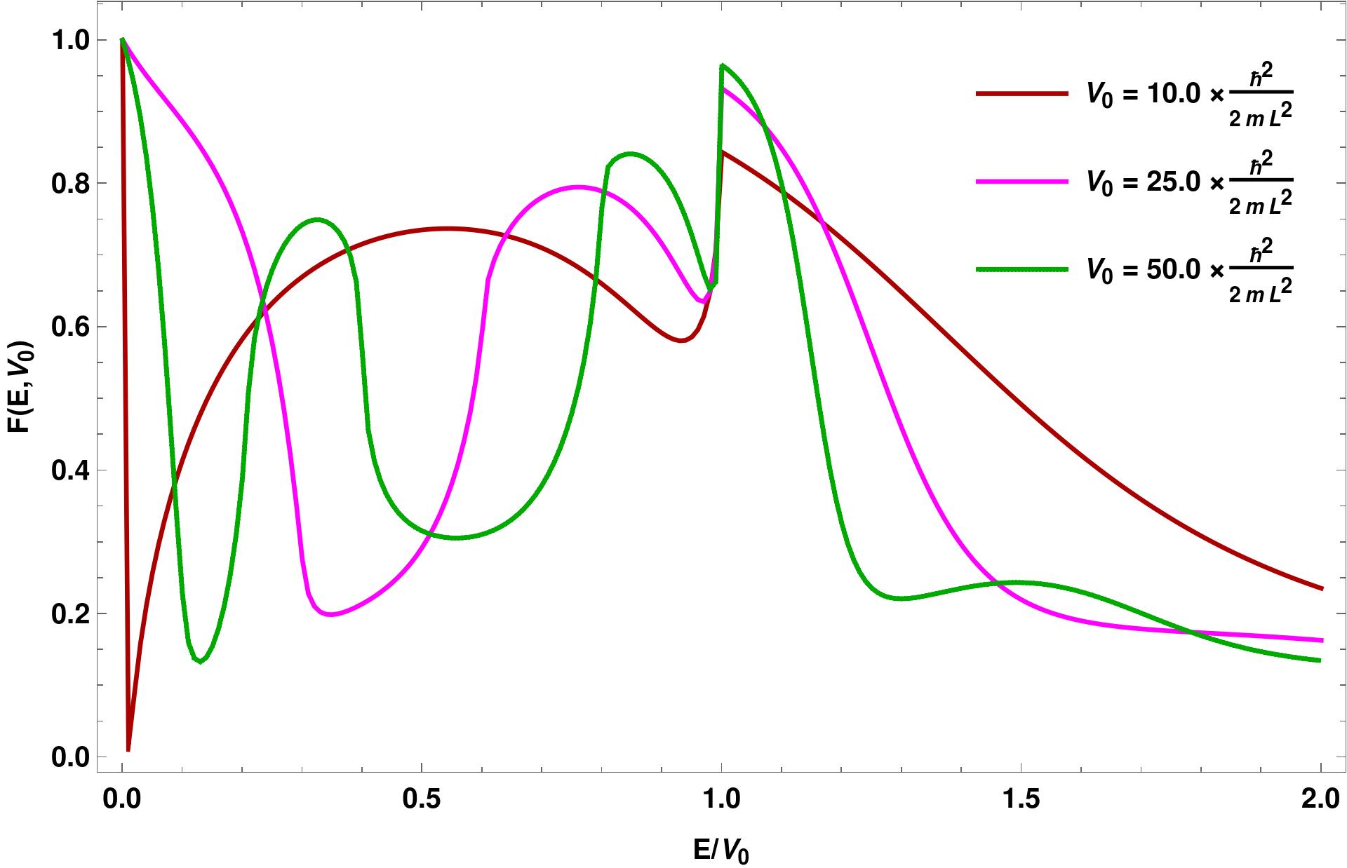
Figure 7: 3d QBCP: Plots of the (a) conductivity ($\sigma$ in units of $8\pi^{2}$), and (b) Fano factor ($F$), as functions of $E/V_{0}$, for various values of $V_{0}$.

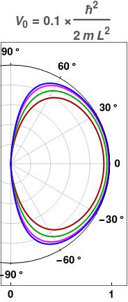
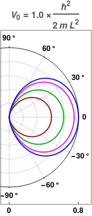
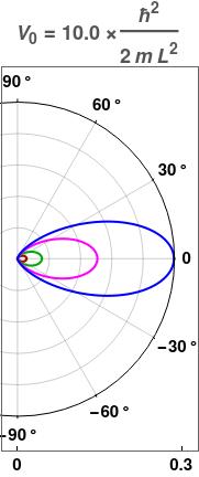
Figure 8: Normal metal: The polar plots show the transmission coefficient $T(E,V_{0},\phi)\big{|}_{E<V_{0}}$ as functions of the incident angle $\phi$ for the parameters $E=0.3\,V_{0}$ (red), $E=0.5\,V_{0}$ (green), $E=0.8\,V_{0}$ (magenta) and $E=1.0\,V_{0}$ (blue).

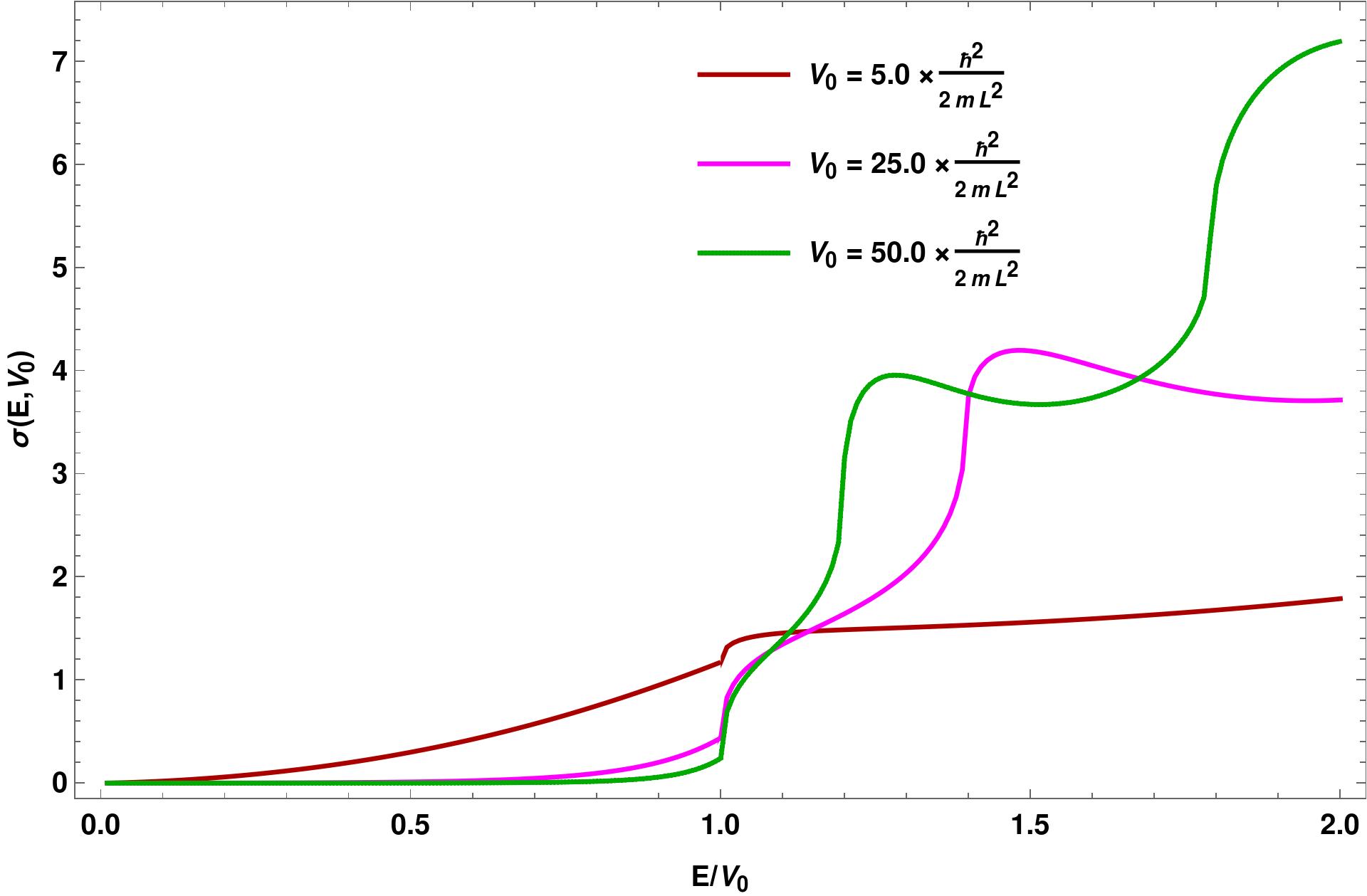
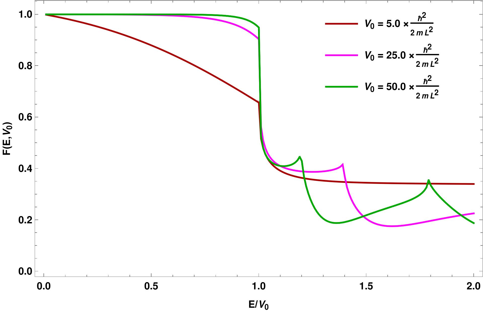
Figure 9: 2d normal metal: Plots of the (a) conductivity ($\sigma$ in units of $2\pi$), and (b) Fano factor ($F$), as functions of $E/V_{0}$, for various values of $V_{0}$.

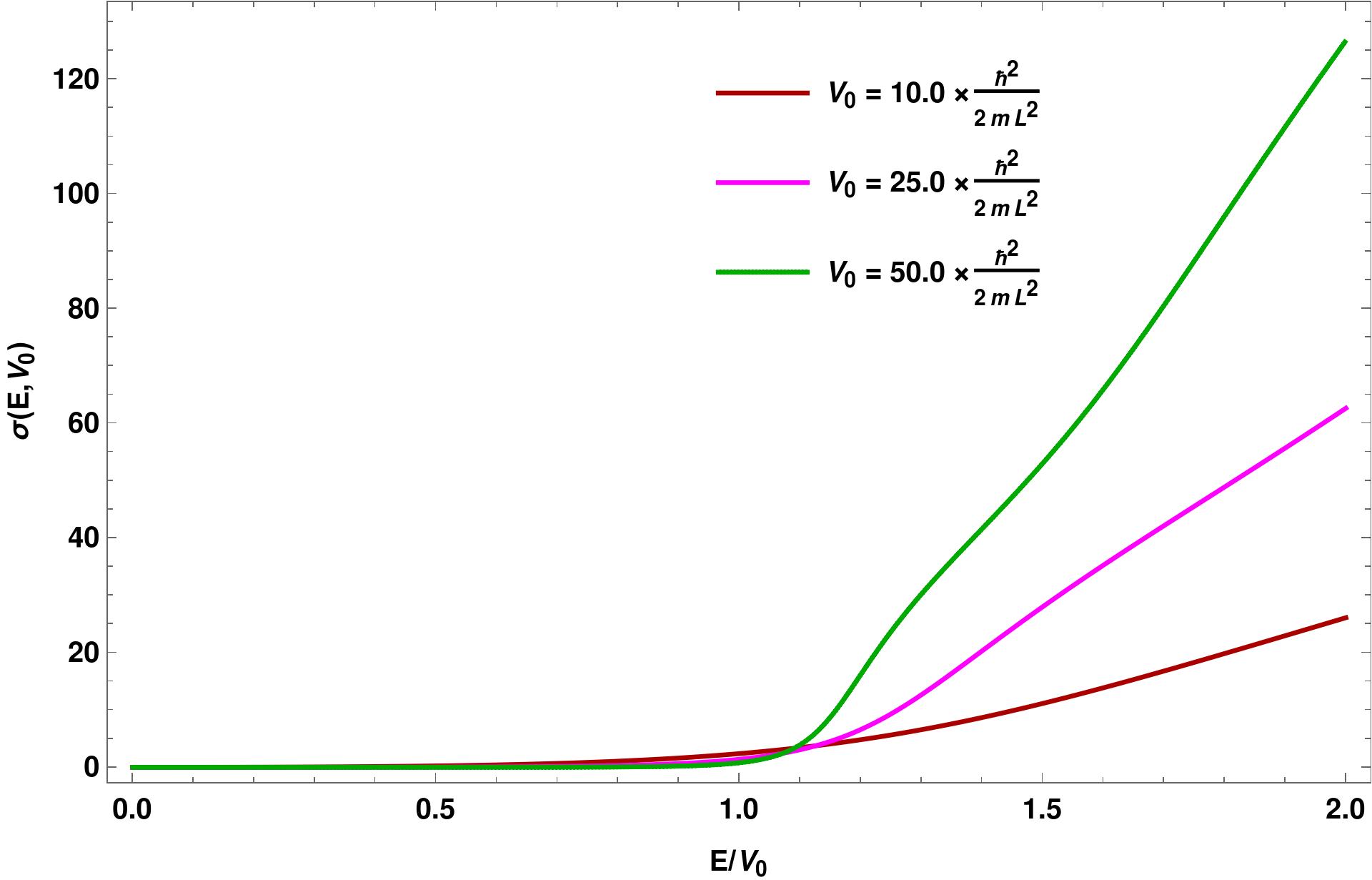
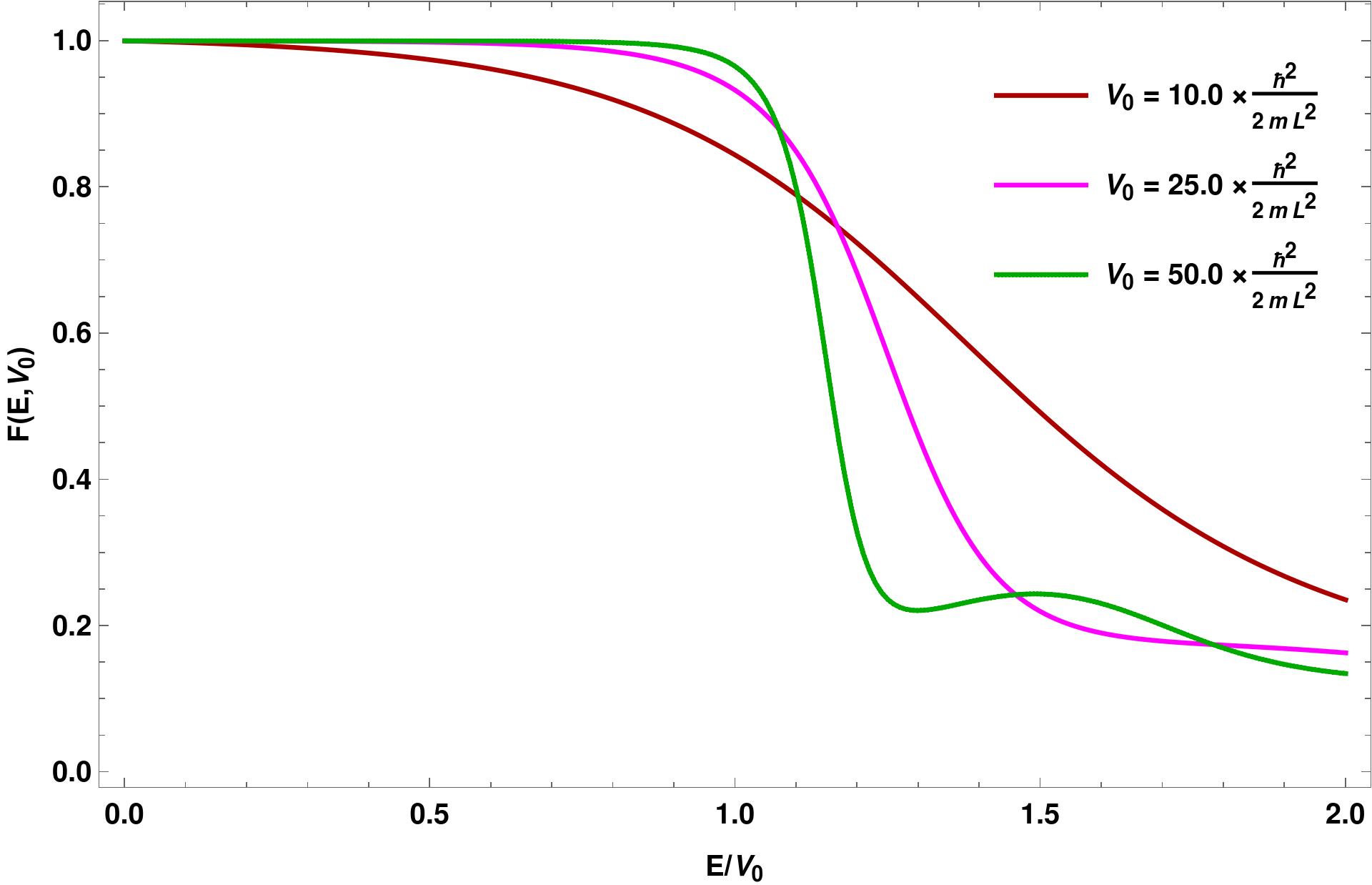
Figure 10: 3d normal metal: Plots of the (a) conductivity ($\sigma$ in units of $2\pi^{2}$), and (b) Fano factor ($F$), as functions of $E/V_{0}$, for various values of $V_{0}$.

IV Comparison with the the results for electrons in normal metals

We compare the results obtained for QBCP semimetals with those in normal metals. For normal metals, we have only one electron band to consider where the Fermi energy will intersect (irrespective of the height of the barrier). Using the continuity of the wavefunctions and their $x$-derivatives at the two ends of the barrier, we can easily find the transmission coefficient to be always given by:

$$t(E,V_{0}) =\frac{2\,\mathrm{i}\,\tilde{k}\,k_{\ell}}{\left(\tilde{k}^{2}+\,k_{\ell}^{2}\right)\sin\left(\tilde{k}L\right)+2\,\mathrm{i}\,\tilde{k}\,\,k_{\ell}\cos\left(\tilde{k}L\right)}\,,$$ (34)

independent of whether $E<V_{0}$ or $E>V_{0}$. As expected, this expression varies from the QBCP case only in the $E<V_{0}$ regime, as whenever $E>V_{0}$, a quasiparticle excitation moves across the barrier in the same way as a normal metal electron does.

In Fig. 8, we show the plots of the transmission amplitude $T(E,V_{0},\phi)=|t(E,V_{0})|^{2}$ as function of the angle $\phi$, for the normal metal (in the 2d case, or 3d case with $k_{z}=0$). We also show the behaviour of conductivity and Fano factor for 2d and 3d normal electrons in Figs. 9 and 10 respectively. As expected, Fig. 9 differs from Fig. 4, or Fig. 10 differs from Fig. 7, only in the regions where $E<V_{0}$.

V Summary and Discussions

From our computations of the tunneling coefficients for the 2d and 3d QBCP semimetals, we have shown that they exhibit different characteristics than those expected for normal metals. The answers also differ from those expected for graphene [16] and three-band pseudospin-$1$ semimetals [17, 18]. In particular, QBCPs do not exhibit either Klein or super-Klein tunneling [18]. We also note that the transport characteristics for the 2d and 3d QBCP cases show significant differences among themselves. All these observations can be used in experiments to identify the QBCP semimetals.

In future, it will be useful to look at these transport properties in the presence of disorder [21, *ipsita-rahul, *ips-qbt-sc] (as has been done in the case of Weyl [24] and double-Weyl [25] nodes) and/or magnetic fields [26, 27]. Another direction is to examine the effects of anisotropy as well as particle-hole symmetry-breaking terms. This exercise also needs to be carried out in presence of interactions, which can destroy the quantization of various physical quantities in the topological phases [28, 29]. Yet another direction is to explore the time-dependent transport properties when subjected to a time-dependent potential [30], using the Floquet scattering theory, and find out if Fano resonance can occur via quasibound states.

VI Acknowledgments

We thank Emil J. Bergholtz for useful discussions, and Atri Bhattacharya for help with the figures.

References

- Sun et al. [2009] K. Sun, H. Yao, E. Fradkin, and S. A. Kivelson, Topological insulators and nematic phases from spontaneous symmetry breaking in 2d fermi systems with a quadratic band crossing, Phys. Rev. Lett. 103, 046811 (2009).
- Tsai et al. [2015] W.-F. Tsai, C. Fang, H. Yao, and J. Hu, Interaction-driven topological and nematic phases on the lieb lattice, New Journal of Physics 17, 055016 (2015).
- Mandal and Gemsheim [2019] I. Mandal and S. Gemsheim, Emergence of topological Mott insulators in proximity of quadratic band touching points, Condensed Matter Physics 22, 13701 (2019).
- Abrikosov [1974] A. A. Abrikosov, Calculation of critical indices for zero-gap semiconductors, JETP 39, 709 (1974).
- Kondo et al. [2015] T. Kondo, M. Nakayama, R. Chen, J. J. Ishikawa, E. G. Moon, T. Yamamoto, Y. Ota, W. Malaeb, H. Kanai, Y. Nakashima, Y. Ishida, R. Yoshida, H. Yamamoto, M. Matsunami, S. Kimura, N. Inami, K. Ono, H. Kumigashira, S. Nakatsuji, L. Balents, and S. Shin, Quadratic fermi node in a 3d strongly correlated semimetal, Nat Commun 6 (2015).
- Moon et al. [2013] E.-G. Moon, C. Xu, Y. B. Kim, and L. Balents, Non-fermi-liquid and topological states with strong spin-orbit coupling, Phys. Rev. Lett. 111, 206401 (2013).
- Yanagishima and Maeno [2001] D. Yanagishima and Y. Maeno, Metal-nonmetal changeover in pyrochlore iridates, Journal of the Physical Society of Japan 70, 2880 (2001).
- Matsuhira et al. [2007] K. Matsuhira, M. Wakeshima, R. Nakanishi, T. Yamada, A. Nakamura, W. Kawano, S. Takagi, and Y. Hinatsu, Metal–insulator transition in pyrochlore iridates ln2ir2o7 (ln = nd, sm, and eu), Journal of the Physical Society of Japan 76, 043706 (2007).
- Abrikosov and Beneslavskiǐ [1971] A. A. Abrikosov and S. D. Beneslavskiǐ, Possible Existence of Substances Intermediate Between Metals and Dielectrics, Soviet Journal of Experimental and Theoretical Physics 32, 699 (1971).
- Boettcher and Herbut [2016] I. Boettcher and I. F. Herbut, Superconducting quantum criticality in three-dimensional luttinger semimetals, Phys. Rev. B 93, 205138 (2016).
- Luttinger [1956] J. M. Luttinger, Quantum theory of cyclotron resonance in semiconductors: General theory, Phys. Rev. 102, 1030 (1956).
- Murakami et al. [2004] S. Murakami, N. Nagaosa, and S.-C. Zhang, non-abelian holonomy and dissipationless spin current in semiconductors, Phys. Rev. B 69, 235206 (2004).
- Salehi and Jafari [2015] M. Salehi and S. Jafari, Quantum transport through 3d dirac materials, Annals of Physics 359, 64 (2015).
- Tworzydło et al. [2006] J. Tworzydło, B. Trauzettel, M. Titov, A. Rycerz, and C. W. J. Beenakker, Sub-poissonian shot noise in graphene, Phys. Rev. Lett. 96, 246802 (2006).
- Blanter and Büttiker [2000] Y. Blanter and M. Büttiker, Shot noise in mesoscopic conductors, Physics Reports 336, 1 (2000).
- Katsnelson et al. [2006] M. I. Katsnelson, K. S. Novoselov, and A. K. Geim, Chiral tunnelling and the Klein paradox in graphene, Nature Physics 2, 620 (2006).
- Fang et al. [2016] A. Fang, Z. Q. Zhang, S. G. Louie, and C. T. Chan, Klein tunneling and supercollimation of pseudospin-1 electromagnetic waves, Phys. Rev. B 93, 035422 (2016).
- Zhu and Hui [2017] R. Zhu and P. M. Hui, Shot noise and fano factor in tunneling in three-band pseudospin-1 dirac–weyl systems, Physics Letters A 381, 1971 (2017).
- Janssen and Herbut [2015] L. Janssen and I. F. Herbut, Nematic quantum criticality in three-dimensional fermi system with quadratic band touching, Phys. Rev. B 92, 045117 (2015).
- Herbut [2012] I. F. Herbut, Isospin of topological defects in dirac systems, Phys. Rev. B 85, 085304 (2012).
- Nandkishore and Parameswaran [2017] R. M. Nandkishore and S. A. Parameswaran, Disorder-driven destruction of a non-fermi liquid semimetal studied by renormalization group analysis, Phys. Rev. B 95, 205106 (2017).
- Mandal and Nandkishore [2018] I. Mandal and R. M. Nandkishore, Interplay of coulomb interactions and disorder in three-dimensional quadratic band crossings without time-reversal symmetry and with unequal masses for conduction and valence bands, Phys. Rev. B 97, 125121 (2018).
- Mandal [2018] I. Mandal, Fate of superconductivity in three-dimensional disordered luttinger semimetals, Annals of Physics 392, 179 (2018).
- Sbierski et al. [2014] B. Sbierski, G. Pohl, E. J. Bergholtz, and P. W. Brouwer, Quantum transport of disordered weyl semimetals at the nodal point, Phys. Rev. Lett. 113, 026602 (2014).
- Sbierski et al. [2017] B. Sbierski, M. Trescher, E. J. Bergholtz, and P. W. Brouwer, Disordered double weyl node: Comparison of transport and density of states calculations, Phys. Rev. B 95, 115104 (2017).
- Yesilyurt et al. [2016] C. Yesilyurt, S. G. Tan, G. Liang, and M. B. A. Jalil, Klein tunneling in weyl semimetals under the influence of magnetic field, Scientific Reports 6, 38862 (2016).
- Mandal [2020a] I. Mandal, Transmission in pseudospin-1 and pseudospin-3/2 semimetals with linear dispersion through scalar and vector potential barriers, Physics Letters A 384, 126666 (2020a).
- Avdoshkin et al. [2020] A. Avdoshkin, V. Kozii, and J. E. Moore, Interactions remove the quantization of the chiral photocurrent at weyl points, Phys. Rev. Lett. 124, 196603 (2020).
- Mandal [2020b] I. Mandal, Effect of interactions on the quantization of the chiral photocurrent for double-weyl semimetals, Symmetry 12, 919 (2020b).
- Zhu and Cai [2017] R. Zhu and C. Cai, Fano resonance via quasibound states in time-dependent three-band pseudospin-1 dirac-weyl systems, Journal of Applied Physics 122, 124302 (2017).