Impact of transforming to Conformal Fermi Coordinates on Quasi-Single Field Non-Gaussianity

Abstract

In general relativity predictions for observable quantities can be expressed in a coordinate independent way. Nonetheless it may be inconvenient to do so. Using a particular frame may be the easiest way to connect theoretical predictions to measurable quantities. For the cosmological curvature bispectrum such frame is described by the Conformal Fermi Coordinates. In single field inflation it was shown that going to this frame cancels the squeezed limit of the density perturbation bispectrum calculated in Global Coordinates. We explore this issue in quasi single field inflation when the curvaton mass and the curvaton-inflaton mixing are small. In this case, the contribution to the bispectrum from the coordinate transformation to Conformal Fermi Coordinates is of the same order as that from the inflaton-curvaton interaction term but does not cancel it.

I Introduction

In standard single field inflationary cosmology starobinskii_spectrum_1979 ; guth_inflationary_1981 ; linde_new_1982 ; linde_coleman-weinberg_1982 ; albrecht_cosmology_1982 the cosmological density perturbations are almost Gaussian maldacena_non-gaussian_2003 . Non-Gaussianities express themselves as connected parts of curvature perturbation correlation functions. The Fourier transform of the three point function of the curvature fluctuations is called the bispectrum and is denoted by $B_{\zeta}({\bf k}_{1},{\bf k}_{2},{\bf k}_{3})$. The bispectrum in standard single field inflation was first calculated by Maldacena maldacena_non-gaussian_2003 in Global Coordinates (GC) and it is suppressed by slow roll parameters.

A phenomenologically relevant limit of the bispectrum is the squeezed limit in which one of the wave-vectors ${\bf q}\equiv{\bf k}_{1}$ is very small in magnitude compared to the other two, $|{\bf q}|\ll|{\bf k}_{2,3}|$. Since ${\bf k}_{1}+{\bf k}_{2}+{\bf k}_{3}=0$ we have that ${\bf k}\equiv{\bf k}_{2}\simeq-{\bf k}_{3}$. The squeezed limit of the bispectrum influences the galaxy power spectrum at small wavevectors dalal_imprints_2008 .

It has been shown tanaka_dominance_2011 ; pajer_observed_2013 ; cabass_how_2017 ; bravo_vanishing_2018 that in standard single field inflation transforming to Conformal Fermi Coordinates (CFC) pajer_observed_2013 ; dai_conformal_2015 with respect to the very long wave-length (small wave-vector) curvature perturbations cancels the squeezed limit of the bispectrum calculated in GC. This cancellation is manifest in the de Sitter era before reheating takes place. Many inflationary models have been studied that can give rise to significant non-Gaussianities, see for example allen_non-gaussian_1987 ; bartolo_non-gaussianity_2002 ; alishahiha_dbi_2004 ; chen_large_2010 ; chen_quasi-single_2010 ; baumann_signature_2012 ; arkani-hamed_cosmological_2015 ; kumar_heavy-lifting_2018 ; deutsch_influence_2018 ; chen_neutrino_2018 ; an_sitter_2019 ; mcaneny_new_2019 ; kumar_cosmological_2019 ; lu_cosmological_2020 ; hook_minimal_2020 . One of the most studied and simplest of these is called Quasi Single Field Inflation (QSFI). It has an additional scalar field called the curvaton that mixes with the inflaton creating a rich dynamics that can lead to measurable curvature non-Gaussianities. We work in the limit where the mass of the curvaton and the coupling between the curvaton and the inflaton are small compared to the Hubble constant during inflation. We calculate the bispectrum in this limit in GC and then transform it to CFC. The contribution from transforming to CFC and from the interaction vertex in GC are typically of the same order but do not cancel against each other. Although QSFI can have large measurable non-Gaussianities, in the limit we work (where the potential interactions of the curvaton are negligible) $f_{\rm NL}$ is only about $10^{-2}$. Throughout this work, we use $G=c=1$ units and $\eta_{\mu\nu}=\operatorname{diag}(-1,+1,+1,+1)$.

II Scale Invariance

In this paper we consider a de Sitter background metric

$$ds^{2}=-dt^{2}+e^{2Ht}dx^{i}dx^{i}\,$$ (1)

and we work in the limit where the Hubble constant during inflation ($H$) and the derivative with respect to the time $t$ of the inflaton field ($\dot{\phi}_{0}$) do not depend on time. Expressing the metric in terms of the conformal time $\tau=-e^{-Ht}/H$, we have

$$ds^{2}=\frac{1}{H^{2}\tau^{2}}\left(-d\tau^{2}+dx^{i}dx^{i}\right)$$ (2)

where the beginning and the end of inflation correspond to, respectively, $\tau\rightarrow-\infty$ and $\bar{\tau}\simeq 0$. The background metric exhibits scale invariance under the transformation $\tau\rightarrow\lambda\tau$ and $x^{i}\rightarrow\lambda x^{i}$ that is preserved when $\dot{\phi}_{0}$ and $H$ are constant. This symmetry implies that the power spectrum is a homogeneous function of order minus three in $1/\tau$ and $|{\bf p}|$. That is,

$$\left(3+\frac{\partial}{\partial{\log{|{\bf p}|}}}\right)P_{\zeta}(\tau,|{\bf p}|)=\frac{\partial}{\partial{\log{\tau}}}P_{\zeta}(\tau,|{\bf p}|)\,.$$ (3)

In this paper we will neglect the time evolution of $H$ and ${\dot{\phi}}_{0}$ that is important towards the end of inflation and depends on the shape of the inflaton potential. Hence all our results will be scale invariant. Scale invariance has implications for the higher point correlations of the curvature fluctuations as well. For example, it implies that the bispectrum $B_{\zeta}(\tau,{\bf k}_{1},{\bf k}_{2},{\bf k}_{3})$ is a homogeneous function of ${\bf k}_{1},{\bf k}_{2},{\bf k}_{3}$ and $1/\tau$ of degree minus six.

III Quasi Single Field Inflation

In QSFI the inflaton field $\phi$ is accompanied by another scalar field the curvaton $s$. Although $s$ does not participate in the slow roll process, it does interact and mix with the inflaton through the term assassi_planck-suppressed_2014 ; an_non-gaussian_2018

$${\cal L}_{{\rm dim}~{}5}=-\frac{1}{\Lambda}{g^{\mu\nu}\partial_{\mu}\phi\partial_{\nu}\phi}s\,.$$ (4)

We work in the gauge where the inflaton field is only a function of time $\phi_{0}(t)$ with no fluctuations. The Goldstone field $\pi(x)$, associated with time translational invariance breaking (by the time dependence of $\phi_{0}$) cheung_effective_2008 gives rise to the curvature fluctuations $\zeta$ which are linearly related to $\pi$ via

$$\zeta=-{\frac{H}{\dot{\phi}_{0}}}\pi\,.$$ (5)

In a de Sitter background, the Lagrangian describing $\pi(x)$ and $s(x)$ is then

$$\mathcal{L}=\mathcal{L}_{0}+\mathcal{L}_{{\rm int}}\,$$ (6)

where

$$\mathcal{L}_{0}=\frac{1}{2(H\tau)^{2}}\left[\left(\partial_{\tau}\pi\right)^{2}-\nabla\pi\cdot\nabla\pi+(\partial_{\tau}s)^{2}-\frac{m^{2}}{(H\tau)^{2}}s^{2}-\nabla s\cdot\nabla s-\frac{2\mu}{H\tau}s\partial_{\tau}\pi\right]\,$$ (7)

and

$${\cal L}_{\rm int}=\frac{1}{\Lambda(H\tau)^{2}}\left[(\partial_{\tau}\pi)^{2}-{\nabla{\pi}}\cdot{\nabla\pi}\right]s\,.$$ (8)

Note that we have neglected any potential interaction terms for the curvaton $s$. In Eq. (7) we introduced

$$\mu=2{\dot{\phi}_{0}}/{{\Lambda}}$$ (9)

and we rescaled $\pi$ by $\dot{\phi}_{0}$ (we take $\dot{\phi_{0}}>0$) to obtain a more standard normalization for the $\pi$ kinetic term. We have also included the measure factor $\sqrt{-g}$ in the Lagrangian so that the action is equal to $\int d^{3}xd\tau{\cal L}$. The kinetic mixing term between $\pi$ and $s$ in Eq. (7) is the result of the background inflaton field breaking Lorentz invariance. We now introduce the quantities

$$\alpha_{\pm}=\frac{3}{2}\pm\sqrt{\frac{9}{4}-\frac{m^{2}+\mu^{2}}{H^{2}}}\,$$ (10)

and

$$\bar{\eta}=|{\bf k}|\bar{\tau}$$ (11)

where ${\bf k}$ is the wavevector associated to the shortest wavelenght mode that we consider in the bispectrum. We will work in the limit $(m^{2}+\mu^{2})/H^{2}\ll 1$, which implies that

$$\alpha_{-}\simeq\frac{m^{2}+\mu^{2}}{3H^{2}}\ll 1\,.$$ (12)

We also assume that $\mu^{2}/(\mu^{2}+m^{2})=\mathcal{O}(1)$ and

$$\frac{1-(-\bar{\eta})^{\alpha_{-}}}{\alpha_{-}}\gg 1\,.$$ (13)

This last condition is required for the terms we keep in the power spectrum and bispectrum to be enhanced over those that we neglect. Using the methods developed in an_non-gaussian_2018 we compute analytically the equal time correlation functions of the curvature perturbation at the end of inflation.

To compute correlation functions involving $\pi$ and $s$, we expand the quantum fields in terms of creation and annihilation operators. Due to the kinetic mixing term in the Lagrangian, the fields $\pi$ and $s$ share a pair of creation and annihilation operators with commutation relations,

$$[a^{(i)}({\bf p}),{a^{(j)}}^{\dagger}({\bf p^{\prime}})]=(2\pi)^{3}\delta^{ij}\delta^{(3)}({\bf p-p^{\prime}})\,.$$ (14)

Introducing $\eta=|{\bf p}|\tau$ we write

$$\pi({\bf x},\tau)=\int\frac{d^{3}p}{(2\pi)^{3}}\left(a^{(1)}({\bf p})\pi_{|\bf p|}^{(1)}(\eta)e^{i{\bf p}\cdot{\bf x}}+a^{(2)}({\bf p})\pi_{|\bf p|}^{(2)}(\eta)e^{i{\bf p}\cdot{\bf x}}+{\rm h.c.}\right)\,$$ (15)

and

$$s({\bf x},\tau)=\int\frac{d^{3}p}{(2\pi)^{3}}\left(a^{(1)}({\bf p}){s}_{|\bf p|}^{(1)}(\eta)e^{i{\bf p}\cdot{\bf x}}+a^{(2)}({\bf p}){s}_{|\bf p|}^{(2)}(\eta)e^{i{\bf p}\cdot{\bf x}}+{\rm h.c.}\right)\,.$$ (16)

The mode functions $\pi_{|\bf p|}^{(i)}(\eta)$ and $s_{|\bf p|}^{(i)}(\eta)$ are determined by the equations of motion for the fields $\pi$ and $s$ and by the canonical commutation relations. For the calculation of the bispectrum when $\alpha_{-}$ is small it is the behaviour of these mode functions for $-\eta$ close to zero that is important an_non-gaussian_2018 . After rescaling the mode functions

$$\pi^{(i)}_{|\bf p|}(\eta) = \frac{H}{{|\bf p|}^{3/2}}\pi^{(i)}(\eta)\,,$$ (17)

$$s^{(i)}_{|\bf p|}(\eta) = \frac{H}{{|\bf p|}^{3/2}}s^{(i)}(\eta)\,$$ (18)

we can expand $\pi^{(i)}(\eta)$ and $s^{(i)}(\eta)$ in this region as

$$\pi^{(i)}(\eta) =a^{(i)}_{0}+a^{(i)}_{-}(-\eta)^{\alpha_{-}}+a^{(i)}_{0,2}(-\eta)^{2}+a^{(i)}_{-,2}(-\eta)^{\alpha_{-}+2}+a^{(i)}_{+}(-\eta)^{\alpha_{+}}+a^{(i)}_{3}(-\eta)^{3}+\dots\,,$$ (19)

$$s^{(i)}(\eta) =b^{(i)}_{-}(-\eta)^{\alpha_{-}}+b^{(i)}_{0,2}(-\eta)^{2}+b^{(i)}_{-,2}(-\eta)^{\alpha_{-}+2}+b^{(i)}_{+}(-\eta)^{\alpha_{+}}+b^{(i)}_{3}(-\eta)^{3}+\dots$$ (20)

where the ellipses represent terms with higher powers of $-\eta$ that we will not need. Using the equations of motion we get

$$b^{(i)}_{0}=0,\quad b^{(i)}_{-}=\frac{Ha^{(i)}_{-}\alpha_{-}}{\mu},\quad b^{(i)}_{+}=\frac{Ha^{(i)}_{+}\alpha_{+}}{\mu},\quad b^{(i)}_{3}=\frac{-3H\mu}{m^{2}}a^{(i)}_{3}\,.$$ (21)

By matching this theory to an effective field theory in the small $-\eta$ limit an_non-gaussian_2018 it is possible to prove that

$$\sum_{i=1,2}|a_{0}^{(i)}|^{2}=\sum_{i=1,2}|a_{-}^{(i)}|^{2}=-\sum_{i=1,2}{\rm Re}[a_{0}^{(i)}a_{-}^{(i)*}]=\frac{9\mu^{2}H^{2}}{2(\mu^{2}+m^{2})^{2}}\,$$ (22)

and by using the canonical commutation relations for the fields $\pi$ and $s$ we find

$${\rm Im}[a_{0}^{(i)}b_{3}^{(i)*}]=\frac{\mu H}{2(\mu^{2}+m^{2})},\quad{\rm Im}[a_{-}^{(i)*}b_{+}^{(i)*}]=-\frac{\mu H}{2(\mu^{2}+m^{2})}\,.$$ (23)

All other similar quantities are subleading in our calculations. Using the above results the leading contribution to the power spectrum of the curvature perturbations in the limit of small $-\eta$ is

$$P_{\zeta}(\tau,|{\bf p}|)=\frac{9H^{6}\mu^{2}\left[1-(-\eta)^{\alpha_{-}}\right]^{2}}{2|{\bf p}|^{3}\dot{\phi}_{0}^{2}\left(\mu^{2}+m^{2}\right)^{2}}\,.$$ (24)

This is needed to compute the impact of the change of coordinates from GC to CFC on the bispectrum (see the Appendix A).

IV Bispectrum in Global Coordinates

In this section we work in GC and we compute the bispectrum for $\zeta$ in the squeezed limit at the end of inflation. Working to first order in the interactions and using the in-in formalism weinberg_quantum_2005 we have

$$\langle\zeta({\bar{\tau},\bf x}_{1})\zeta(\bar{\tau},{\bf x}_{2})\zeta(\bar{\tau},{\bf x}_{3})\rangle=i\int_{-\infty}^{\bar{\tau}}d\tau^{\prime}\langle[H_{\rm int}(\tau^{\prime}),\zeta(\bar{\tau},{\bf x}_{1})\zeta(\bar{\tau},{\bf x}_{2})\zeta(\bar{\tau},{\bf x}_{3})]\rangle$$ (25)

where $H_{\rm int}$ denotes the interaction Hamiltonian in the interaction picture. In the squeezed limit we can drop the terms proportional to the spatial derivatives of $\pi$ from $\mathcal{L}_{\rm int}$ and the interaction Hamiltonian simplifies to

$$H_{\rm int}(\tau)=\int d^{3}x\frac{1}{(H\tau)^{2}\Lambda}(\partial_{\tau}\pi)^{2}s\,.$$ (26)

Notice that $H_{\rm int}=\mathcal{L}_{\rm int}$ since we have a derivative interaction. Fourier transforming we find that the leading order contribution in $\alpha_{-}$ in the region of phase space that we are considering to the bispectrum in the squeezed limit is

$$B_{\zeta}^{(\rm GC)}({\bf q},{\bf k},{-\bf k})\simeq-4\left(\frac{H^{7}\mu}{{\dot{\phi}}_{0}^{4}}\right)\frac{1}{|{\bf k}|^{3}|{\bf q}|^{3}}\left(I_{a}+I_{b}+I_{c}\right)$$ (27)

where

$$I_{a}=\int_{-1}^{\bar{\eta}}\frac{d\eta^{\prime}}{(-\eta^{\prime})^{2}}{\rm Re}\left[\pi^{(i)}\left(r\bar{\eta}\right)\dot{\pi}^{(i)}\left(r\eta^{\prime}\right)^{*}\right]{\rm Re}\left[\pi^{(j)}(\bar{\eta})\dot{\pi}^{(j)}\left(\eta^{\prime}\right)^{*}\right]{\rm Im}\left[\pi^{(n)}(\bar{\eta}){s}^{(n)}\left(\eta^{\prime}\right)^{*}\right],$$ (28)

$$I_{b}=\int_{-1}^{\bar{\eta}}\frac{d\eta^{\prime}}{(-\eta^{\prime})^{2}}{\rm Re}\left[\pi^{(i)}\left(r\bar{\eta}\right)\dot{\pi}^{(i)}\left(r\eta^{\prime}\right)^{*}\right]{\rm Im}\left[\pi^{(j)}(\bar{\eta})\dot{\pi}^{(j)}\left(\eta^{\prime}\right)^{*}\right]{\rm Re}\left[\pi^{(n)}(\bar{\eta}){s}^{(n)}\left(\eta^{\prime}\right)^{*}\right],$$ (29)

and

$$I_{c}=\int_{-1}^{\bar{\eta}}\frac{d\eta^{\prime}}{(-\eta^{\prime})^{2}}{\rm Re}\left[\pi^{(i)}\left(\bar{\eta}\right)\dot{\pi}^{(i)}\left(\eta^{\prime}\right)^{*}\right]{\rm Im}\left[\pi^{(j)}(\bar{\eta})\dot{\pi}^{(j)}\left(\eta^{\prime}\right)^{*}\right]{\rm Re}\left[\pi^{(n)}\left(r\bar{\eta}\right){s}^{(n)}\left(r\eta^{\prime}\right)^{*}\right]\,.$$ (30)

In the above equations a dot indicates a derivative with respect to $\eta^{\prime}$, the repeated mode function indices $i,j,n$ are summed over $1$ and $2$ and we introduced the parameter $r\equiv{|{\bf q}|}/{|{\bf k}|}$. Most of the contribution to the integrals comes from the region $-\eta^{\prime}\ll 1$ and to leading order in $(\mu^{2}+m^{2})/H^{2}$ we set the lower bound of the integrals to be $-1$. Using the results of Section III we find that

$${\rm Re}\left[\pi^{(i)}\left(r\bar{\eta}\right)\dot{\pi}^{(i)}\left(r\eta^{\prime}\right)^{*}\right]\simeq\frac{1}{2}\left(\frac{3\mu^{2}}{\mu^{2}+m^{2}}\right)(-\eta^{\prime})^{\alpha_{-}-1}r^{\alpha_{-}}\left[1-\left(-r\bar{\eta}\right)^{\alpha_{-}}\right]\,,$$ (31)

$${\rm Re}\left[\pi^{(i)}\left(\bar{\eta}\right)\dot{\pi}^{(i)}\left(\eta^{\prime}\right)^{*}\right]\simeq\frac{1}{2}\left(\frac{3\mu^{2}}{\mu^{2}+m^{2}}\right)(-\eta^{\prime})^{\alpha_{-}-1}\left[1-\left(-\bar{\eta}\right)^{\alpha_{-}}\right]\,,$$ (32)

$${\rm Im}\left[\pi^{(i)}\left(\bar{\eta}\right){s}^{(i)}\left(\eta^{\prime}\right)^{*}\right]\simeq\frac{1}{2}\left(\frac{H\mu}{\mu^{2}+m^{2}}\right)\left[(-\eta^{\prime})^{3}-(-\eta^{\prime})^{3-\alpha_{-}}(-\bar{\eta})^{\alpha_{-}}\right]\,,$$ (33)

$${\rm Re}\left[\pi^{(i)}\left(r\bar{\eta}\right){s}^{(i)}\left(r\eta^{\prime}\right)^{*}\right]\simeq\frac{3H\mu\left[(-r\bar{\eta})^{\alpha_{-}}-1\right](-r\eta^{\prime})^{\alpha_{-}}}{2\left(\mu^{2}+m^{2}\right)}\,,$$ (34)

$${\rm Re}\left[\pi^{(i)}\left(\bar{\eta}\right){s}^{(i)}\left(\eta^{\prime}\right)^{*}\right]\simeq\frac{3H\mu\left[(-\bar{\eta})^{\alpha_{-}}-1\right](-\eta^{\prime})^{\alpha_{-}}}{2\left(\mu^{2}+m^{2}\right)}\,,$$ (35)

$${\rm Im}\left[\pi^{(i)}\left(\bar{\eta}\right)\dot{\pi}^{(i)}\left(\eta^{\prime}\right)^{*}\right]\simeq\frac{\eta^{\prime 2}\left[\mu^{2}\left(\frac{\eta^{\prime}}{\bar{\eta}}\right)^{-\alpha_{-}}+m^{2}\right]}{2\left(\mu^{2}+m^{2}\right)}\,,$$ (36)

and that ${\rm Im}\left[\pi^{(i)}\left(r\bar{\eta}\right){s}^{(i)}\left(r\eta^{\prime}\right)^{*}\right]$ and ${\rm Im}\left[\pi^{(i)}\left(r\bar{\eta}\right)\dot{\pi}^{(i)}\left(r\eta^{\prime}\right)^{*}\right]$ are suppressed in the squeezed limit. Performing the $\eta^{\prime}$ integration we have that to leading order in small quantities

$$I_{a}=\frac{27H^{3}\mu^{5}\left[(-\bar{\eta})^{\alpha_{-}}-1\right]^{3}r^{\alpha_{-}}\left[(-r\bar{\eta})^{\alpha_{-}}-1\right]}{16\left(\mu^{2}+m^{2}\right)^{4}}$$ (37)

and

$$I_{b}=I_{c}=\frac{27H^{3}\mu^{3}\left[(-\bar{\eta})^{\alpha_{-}}-1\right]^{2}r^{\alpha_{-}}\left[(-r\bar{\eta})^{\alpha_{-}}-1\right]\left[(-\bar{\eta})^{\alpha_{-}}\left(2\mu^{2}+m^{2}\right)+m^{2}\right]}{16\left(\mu^{2}+m^{2}\right)^{4}}\,.$$ (38)

This completes the calculation of the bispectrum in GC and we now turn to transform it to CFC.

V The Bispectrum in CFC

We are now ready to compute the bispectrum in CFC by using Eq. (68) to transform the result that we found in Section IV for the bispectrum in GC. We have

$$B_{\zeta}({\bf q},{\bf k},-{\bf k})=B^{(\rm GC)}_{\zeta}({\bf q},{\bf k},-{\bf k})+\Delta B_{\zeta}({\bf q},{\bf k},-{\bf k})\,$$ (39)

where

$$\Delta B_{\zeta}({\bf q},{\bf k},-{\bf k})=P_{\zeta}(\bar{\tau},|{\bf q}|)\frac{\partial}{\partial\log\bar{\tau}}P_{\zeta}(\bar{\tau},|{\bf k}|)\,$$ (40)

and to simplify the notation we dropped the superscript $\rm CFC$. Using Eq (24) we get

$$\Delta B_{\zeta}({\bf q},{\bf k},-{\bf k})\simeq\frac{27H^{10}\mu^{4}\left[(-\bar{\eta})^{\alpha_{-}}-1\right](-\bar{\eta})^{\alpha_{-}}\left[(-r\bar{\eta})^{\alpha_{-}}-1\right]^{2}}{2|{\bf k}|^{3}|{\bf q}|^{3}\dot{\phi}_{0}^{4}\left(\mu^{2}+m^{2}\right)^{3}}\,.$$ (41)

Even though for modes of cosmological interest $-\bar{\eta}=-|{\bf k}|\bar{\tau}\simeq e^{-60}$ baumann_tasi_2012 , $(-\bar{\eta})^{\alpha_{-}}$ can still be of order unity, for example if $\alpha_{-}\sim 1/50$. In this case, the contribution to the bispectrum from the change of coordinates from GC to CFC, is comparable to the one that comes from the three point vertex in GC.

In the limit $m\ll\mu$, we finally obtain

$$B^{(\rm GC)}_{\zeta}({\bf q},{\bf k},-{\bf k})=-\frac{1}{{|{\bf k}|}^{3}{|{\bf q}|}^{3}}\frac{27H^{10}\left[(-\bar{\eta})^{{\alpha_{-}}}-1\right]^{2}\left[5(-\bar{\eta})^{{\alpha_{-}}}-1\right]r^{{\alpha_{-}}}\left[(-r\bar{\eta})^{{\alpha_{-}}}-1\right]}{4\mu^{2}{\dot{\phi}}_{0}^{4}}$$ (42)

and

$$\Delta B_{\zeta}({\bf q},{\bf k},-{\bf k})\simeq\frac{27H^{10}\left[(-\bar{\eta})^{\alpha_{-}}-1\right](-\bar{\eta})^{\alpha_{-}}\left[(-r\bar{\eta})^{\alpha_{-}}-1\right]^{2}}{2|{\bf k}|^{3}|{\bf q}|^{3}\dot{\phi}_{0}^{4}\mu^{2}}\,$$ (43)

that are plotted in Fig. 1. Notice that the leading contribution to the bispectrum in GC vanishes for $(-\bar{\eta})^{\alpha_{-}}=0.2$. At this point the part from the change of coordinates dominates the bispectrum.

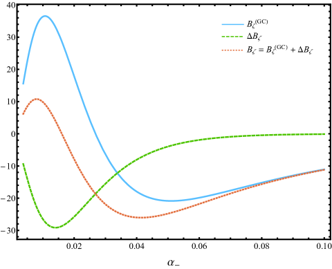
Figure 1: Contributions to the Bispectrum for $m\ll\mu$, $-\bar{\eta}=e^{-60}$ and $r=10^{-3}$. We consider values of $\alpha_{-}$ that go from $0.0037$ (corresponding to $(-\bar{\eta})^{\alpha_{-}}=0.8$) to $\alpha_{-}=0.1$. The $y$-axis is in units of $H^{8}/(|{\bf k}|^{3}|{\bf q}|^{3}{\dot{\phi}}_{0}^{4})$.

In Fig. 2 we plot the local bispectrum $f_{\rm NL}$ in GC and CFC as a function of $\alpha_{-}$ where

$$f_{\rm NL}^{(\rm GC)}=\frac{5}{12}\frac{B^{(\rm GC)}_{\zeta}({\bf q},{\bf k},-{\bf k})}{P_{\zeta}(\bar{\tau},|{\bf k}|)P_{\zeta}(\bar{\tau},|{\bf q}|)}\,,$$ (44)

$$\Delta f_{\rm NL}=\frac{5}{12}\frac{\Delta B_{\zeta}({\bf q},{\bf k},-{\bf k})}{P_{\zeta}(\bar{\tau},|{\bf k}|)P_{\zeta}(\bar{\tau},|{\bf q}|)}\,$$ (45)

and in the limit $m\ll\mu$ we have

$$f_{\rm NL}^{(\rm GC)} = -\frac{5\alpha_{-}r^{\alpha_{-}}\left[5(-\bar{\eta})^{\alpha_{-}}-1\right]}{12\left[(-r\bar{\eta})^{\alpha_{-}}-1\right]}\,,$$ (46)

$$\Delta f_{\rm NL} = \frac{5\alpha_{-}(-\bar{\eta})^{\alpha_{-}}}{6\left[(-\eta)^{\alpha_{-}}-1\right]}\,.$$ (47)

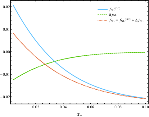
Figure 2: Contributions to $f_{\rm NL}$ for $m\ll\mu$, $-\bar{\eta}=e^{-60}$ and $r=10^{-3}$. We consider values of $\alpha_{-}$ that go from $0.0037$ (corresponding to $(-\bar{\eta})^{\alpha_{-}}=0.8$) to $\alpha_{-}=0.1$.

Both $B|{\bf k}|^{3}|{\bf q}|^{3}$ and $f_{\rm NL}$ depend very weekly on the value of $r$. This is because $r$ only enters in these quantities raised to the power $\alpha_{-}$.

VI Concluding Remarks

In this paper we considered QSFI where a dimension five operator couples the inflaton and the curvaton field. Working in the limit of small coupling and small curvaton mass we computed analytically the bispectrum in the squeezed limit in GC and in CFC. We found that transforming to CFC introduces a non-negligible correction to the result in GC. We also showed that $f_{\rm NL}$ can be either enhanced or suppressed by this effect, and in the region of parameter space that we considered $f_{\rm NL}\simeq 10^{-2}$. In this model $f_{\rm NL}$ is small and hence these non-Gaussianities could not be observed in the near future. However, this is an interesting example where the change of coordinates from GC to CFC can have an order one effect on the bispectrum.

Appendix A Transformation of the Bispectrum to Conformal Fermi Coordinates

In this Appendix we rederive the coordinate transformation from GC to CFC and compute the bispectrum in CFC. Rather than taking the constructive approach of the previous literature we derive necessary and sufficient conditions that the coordinate transformation must satisfy.

The metric in GC is given by

$$g_{\mu\nu}(x)=a^{2}(\tau)\left[\eta_{\mu\nu}+h_{\mu\nu}(x)\right]\,$$ (48)

and the metric scalar perturbations in $h_{\mu\nu}$ are expressed in terms of the curvature perturbation $\zeta$ as follows

$$h_{00} = -2\frac{\partial_{\tau}\zeta}{\mathcal{H}}\,,$$ (49)

$$h_{0i} = -\partial_{i}\frac{\zeta}{\mathcal{H}}\,,$$ (50)

$$h_{ij} = 2\zeta\delta_{ij}\,,$$ (51)

where $\mathcal{H}\equiv\frac{1}{a}\frac{da}{d\tau}$. We split the metric perturbation as

$$h_{\mu\nu}(x)=h^{L}_{\mu\nu}(x)+h^{S}_{\mu\nu}(x)$$ (52)

where $h^{L}_{\mu\nu}(k)\approx 0$ for $k\gtrsim\Lambda$ and $h^{S}_{\mu\nu}(k)\approx 0$ for $k\lesssim\Lambda$. Here $\Lambda$ is a cutoff that divides the modes into short and long. In CFC with respect to the longest wavelength modes the metric has the form

$$g^{F}_{\mu\nu}(x_{F})=a^{2}(\tau_{F})\left[\eta_{\mu\nu}+h^{S}_{\mu\nu}(x_{F})+\mathcal{O}(x_{F}^{i}x_{F}^{j})\right]\,$$ (53)

where the terms $\mathcal{O}(x_{F}^{i}x_{F}^{j})$ are made negligible by an appropriate choice of CFC. However this choice does not explicitly enter our analysis.

The coordinate transformation that takes us between these two frames can be expanded in $x_{F}^{i}$ as pajer_observed_2013 ; dai_conformal_2015 ; cabass_how_2017 ; bravo_vanishing_2018

$$x^{\mu}(x_{F})=x_{F}^{\mu}+\xi^{\mu}(\tau_{F})+A_{\;i}^{\mu}(\tau_{F})x_{F}^{i}+B^{\mu}_{\;ij}(\tau_{F})x_{F}^{i}x_{F}^{j}+\mathcal{O}(x_{F}^{i}x_{F}^{j}x_{F}^{k})$$ (54)

where $\xi^{\mu},A^{\mu}_{\;i},B^{\mu}_{\;ij}=\mathcal{O}(h^{L}_{\mu\nu})$ and we neglect quantities $\mathcal{O}\left[(h^{L}_{\mu\nu})^{2}\right]$. Without loss of generality, we assume $B^{\mu}_{\;ij}(\tau_{F})=B^{\mu}_{\;ji}(\tau_{F})$. The transformation law for the metric tensor

$$g^{F}_{\mu\nu}(x_{F})=\frac{\partial x^{\alpha}}{\partial x^{\mu}_{F}}\frac{\partial x^{\beta}}{\partial x^{\nu}_{F}}g_{\alpha\beta}(x)\,$$ (55)

gives ten differential equations for $\xi^{\mu},A^{\mu}_{\;i}$ and $B^{\mu}_{\;ij}$ that need to be satisfied in terms of $h^{L}_{\mu\nu}$ in order for $g^{F}_{\mu\nu}(x_{F})$ to have the form of Eq. (53). Requiring each differential equation to hold order by order in $x_{F}^{i}$ gives

$$(\partial_{\tau_{F}}+\mathcal{H})\xi^{0}(\tau_{F}) = -\frac{\partial_{\tau_{F}}\zeta_{L}({\bf x}_{F}={\bf 0},\tau_{F})}{\mathcal{H}(\tau_{F})}$$ (56)

$$(\partial_{\tau_{F}}+\mathcal{H})A_{\;i}^{0}(\tau_{F}) = -\frac{\partial_{\tau_{F}}\partial_{i}\zeta_{L}({\bf x}_{F}={\bf 0},\tau_{F})}{\mathcal{H}(\tau_{F})}$$ (57)

$$A^{0}_{\;i}(\tau_{F})-\partial_{\tau_{F}}\xi_{i}(\tau_{F}) = -\partial_{i}\frac{\zeta_{L}({\bf x}_{F}={\bf 0},\tau_{F})}{\mathcal{H}(\tau_{F})}$$ (58)

$$2B^{0}_{\;ik}(\tau_{F})-\partial_{\tau_{F}}A_{ik}(\tau_{F}) = -\frac{\partial_{k}\partial_{i}\zeta_{L}({\bf x}_{F}={\bf 0},\tau_{F})}{\mathcal{H}(\tau_{F})}$$ (59)

$$A_{ij}(\tau_{F})+A_{ji}(\tau_{F})+2\mathcal{H}\xi^{0}(\tau_{F})\delta_{ij} = -2\zeta_{L}({\bf x}_{F}={\bf 0},\tau_{F})\delta_{ij}$$ (60)

$$B_{ijk}(\tau_{F})+B_{jik}(\tau_{F})+\frac{1}{2}\mathcal{H}A^{0}_{\;k}(\tau_{F})\delta_{ij} = -\partial_{k}\zeta_{L}({\bf x}_{F}={\bf 0},\tau_{F})\delta_{ij}$$ (61)

where the spatial indices were lowered using $\delta_{ij}$ and the quantities on the right hand side are the expressions in comoving coordinates. These are necessary and sufficient conditions for Eq. (53) to hold. With the coordinate transformation at hand we find how the connected three point function of $\zeta$ transforms in going from GC to CFC in the squeezed limit. Following bravo_vanishing_2018 , we have

$$\langle\tilde{\zeta}^{F}(\tau_{F},{\bf k}_{1})\tilde{\zeta}^{F}(\tau_{F},{\bf k}_{2})\tilde{\zeta}^{F}(\tau_{F},{\bf k}_{3})\rangle=\int d^{3}{x}^{F}_{1}d^{3}{x}^{F}_{2}d^{3}{x}^{F}_{3}e^{-i({\bf k}_{1}{\bf x}^{F}_{1}+{\bf k}_{2}{\bf x}^{F}_{2}+{\bf k}_{3}{\bf x}^{F}_{3})}\langle\zeta^{F}(x_{1}^{F})\zeta^{F}(x_{2}^{F})\zeta^{F}(x_{3}^{F})\rangle$$

where $x^{F}_{i}\equiv(\tau_{F},{\bf x}^{F}_{i})$, $|{\bf k}_{1}|\ll|{\bf k}_{2}|,|{\bf k}_{3}|$.

Using spatial translational invariance we get

$$\langle\tilde{\zeta}^{F}(\tau_{F},{\bf k}_{1})\tilde{\zeta}^{F}(\tau_{F},{\bf k}_{2})\tilde{\zeta}^{F}(\tau_{F},{\bf k}_{3})\rangle=(2\pi)^{3}\delta({\bf k}_{1}+{\bf k}_{2}+{\bf k}_{3})B^{(\rm CFC)}_{\zeta}({\bf k}_{1},{\bf k}_{2},{\bf k}_{3})$$ (62)

with

$$B^{(\rm CFC)}_{\zeta}({\bf k}_{1},{\bf k}_{2},{\bf k}_{3}) = \int d^{3}{y}^{F}d^{3}{z}^{F}e^{-i\left[{\bf k}_{1}{\bf y}^{F}+\left({\bf k}_{3}+\frac{{\bf k}_{1}}{2}\right){\bf z}^{F}\right]}\left\langle\zeta^{F}\left(\tau_{F},{\bf y}^{F}\right)\zeta^{F}\left(\tau_{F},-\frac{{\bf z}^{F}}{2}\right)\zeta^{F}\left(\tau_{F},\frac{{\bf z}^{F}}{2}\right)\right\rangle$$ (63)

$$= \int d^{3}{y}^{F}d^{3}{z}^{F}e^{-i\left[{\bf k}_{1}{\bf y}^{F}+({\bf k}_{3}+\frac{{\bf k}_{1}}{2}){\bf z}^{F}\right]}\langle 0_{L}|\zeta_{L}(\tau_{F},{\bf y}^{F})\langle 0_{S}|\zeta_{S}(x_{a})\zeta_{S}(x_{b})|0_{S}\rangle|0_{L}\rangle$$

where $x_{a,b}=x_{a,b}(x_{a,b}^{F})$ and $x^{F}_{a}=(\tau_{F},-{\bf z}^{F}/2)$, $x^{F}_{b}=(\tau_{F},{\bf z}^{F}/2)$  and we assumed that $\zeta$ transforms as a scalar. Moving forward we drop the designation $|0_{S}\rangle$ and write $\langle 0_{S}|\zeta_{S}(x_{a})\zeta_{S}(x_{b})|0_{S}\rangle\equiv\langle\zeta_{S}(x_{a})\zeta_{S}(x_{b})\rangle$ in terms of $x^{F}_{a}$ and $x^{F}_{b}$ up to linear order in $\zeta_{L}$. Eq. (63) implies that the contribution to the three point function is dominated by $|{\bf z}^{F}|\ll 1/|{\bf k}_{3}|$. Thus, using Eq. (54) and working to linear order in the long mode, we find

$$\langle 0_{S}|\zeta_{S}^{F}(x_{a}^{F})\zeta_{S}^{F}(x_{b}^{F})|0_{S}\rangle=\langle 0_{S}|\zeta_{S}(x_{a}^{F})\zeta_{S}(x_{b}^{F})|0_{S}\rangle+\Big{[}\xi^{0}(\tau_{F})\partial_{\tau_{F}}+A^{k}_{\;i}(\tau_{F})({x_{a}^{F}}^{i}-{x_{b}^{F}}^{i})\partial_{k}^{(a)}+$$

$$+\xi^{i}(\tau_{F})(\partial_{i}^{(a)}+\partial_{i}^{(b)})+\frac{1}{2}A^{0}_{\;i}(\tau_{F})({x_{a}^{F}}^{i}+{x_{b}^{F}}^{i})\partial_{\tau_{F}}\Big{]}\langle 0_{S}|\zeta_{S}(\tau_{F},{\bf x}_{a}^{F})\zeta_{S}(\tau_{F},{\bf x}_{b}^{F})|0_{S}\rangle$$ (64)

where the terms on the second line vanish because of translational invariance and because ${\bf x}^{F}_{a}=-{\bf x}^{F}_{b}$. Using Eq. (60) we obtain

$$\langle 0_{S}|\zeta_{S}^{F}(x_{a}^{F})\zeta_{S}^{F}(x_{b}^{F})|0_{S}\rangle=\langle 0_{S}|\zeta_{S}(x_{a}^{F})\zeta_{S}(x_{b}^{F})|0_{S}\rangle+$$ (65)

$$+\left\{\xi^{0}(\tau_{F})\partial_{\tau_{F}}-\left[\mathcal{H}\xi^{0}(\tau_{F})+\zeta_{L}({{\bf 0}},\tau_{F})\right]{\bf z}^{F}\frac{\partial}{\partial{\bf z}^{F}}\right\}\langle 0_{S}|\zeta_{S}(\tau_{F},{\bf z}^{F})\zeta_{S}(\tau_{F},{\bf 0})|0_{S}\rangle\,.$$

Inserting this expression back in Eq. (63) and using rotational invariance we get

$$B^{(\rm CFC)}_{\zeta}({\bf k}_{1},{\bf k}_{2},{\bf k}_{3})=B^{(\rm GC)}_{\zeta}({\bf k}_{1},{\bf k}_{2},{\bf k}_{3})-P_{\zeta}(\tau_{F},|{\bf k}_{1}|)\left(-3-\frac{\partial}{\partial\log|{\bf k}_{3}|}\right)P_{\zeta}(\tau_{F},|{\bf k}_{3}|)$$

$$+\langle\tilde{\zeta}^{F}_{L}(\tau_{F},{\bf k}_{1})\xi^{0}(\tau_{F})\rangle\left[\partial_{\tau_{F}}-\mathcal{H}\left(-3-\frac{\partial}{\partial\log|{\bf k}_{3}|}\right)\right]P_{\zeta}(\tau_{F},|{\bf k}_{3}|)$$ (66)

where

$$\langle\tilde{\zeta}(\tau_{F},{\bf k}_{1})\tilde{\zeta}(\tau_{F},{\bf k}_{2})\tilde{\zeta}(\tau_{F},{\bf k}_{3})\rangle=(2\pi)^{3}\delta({\bf k}_{1}+{\bf k}_{2}+{\bf k}_{3})B^{(\rm GC)}_{\zeta}({\bf k}_{1},{\bf k}_{2},{\bf k}_{3})$$ (67)

and we used that $|{\bf k}_{1}|\ll|{\bf k}_{3}|$. In the limit in which scale invariance is preserved Eq. (3) and the fact that $\mathcal{H}\tau_{F}=-1$ imply that the final result does not depend on the integration constants of Eqs. (56)-(61). We finally obtain

$$B^{(\rm CFC)}_{\zeta}({\bf k}_{1},{\bf k}_{2},{\bf k}_{3})=B^{(\rm GC)}_{\zeta}({\bf k}_{1},{\bf k}_{2},{\bf k}_{3})+P_{\zeta}(\tau_{F},|{\bf k}_{1}|)\frac{\partial}{\partial\log\tau_{F}}P_{\zeta}(\tau_{F},|{\bf k}_{3}|)\,.$$ (68)

This expression coincides with the one in bravo_vanishing_2018 for scale invariant models of inflation.

References

(1)
A. A. Starobinskiǐ, “Spectrum of relict gravitational radiation and the early
state of the universe,” Soviet Journal of Experimental and Theoretical
Physics Letters, vol. 30, p. 682, Dec. 1979.
(2)
A. H. Guth, “Inflationary universe: A possible solution to the horizon and
flatness problems,” Physical Review D, vol. 23, pp. 347–356, Jan.
1981.
Publisher: American Physical Society.
(3)
A. D. Linde, “A new inflationary universe scenario: A possible solution of
the horizon, flatness, homogeneity, isotropy and primordial monopole
problems,” Physics Letters B, vol. 108, pp. 389–393, Feb. 1982.
(4)
A. D. Linde, “Coleman-Weinberg theory and the new inflationary universe
scenario,” Physics Letters B, vol. 114, pp. 431–435, Aug. 1982.
(5)
A. Albrecht and P. J. Steinhardt, “Cosmology for Grand Unified Theories
with Radiatively Induced Symmetry Breaking,” Physical Review
Letters, vol. 48, pp. 1220–1223, Apr. 1982.
Publisher: American Physical Society.
(6)
J. Maldacena, “Non-gaussian features of primordial fluctuations in single
field inflationary models,” Journal of High Energy Physics, vol. 2003,
pp. 013–013, May 2003.
(7)
N. Dalal, O. Doré, D. Huterer, and A. Shirokov, “Imprints of primordial
non-Gaussianities on large-scale structure: Scale-dependent bias and
abundance of virialized objects,” Physical Review D, vol. 77,
p. 123514, June 2008.
(8)
T. Tanaka and Y. Urakawa, “Dominance of gauge artifact in the consistency
relation for the primordial bispectrum,” Journal of Cosmology and
Astroparticle Physics, vol. 2011, pp. 014–014, May 2011.
Publisher: IOP Publishing.
(9)
E. Pajer, F. Schmidt, and M. Zaldarriaga, “The Observed squeezed limit of
cosmological three-point functions,” Physical Review D, vol. 88,
p. 083502, Oct. 2013.
(10)
G. Cabass, E. Pajer, and F. Schmidt, “How Gaussian can our Universe be?,”
Journal of Cosmology and Astroparticle Physics, vol. 2017,
pp. 003–003, Jan. 2017.
arXiv: 1612.00033.
(11)
R. Bravo, S. Mooij, G. A. Palma, and B. Pradenas, “Vanishing of local
non-Gaussianity in canonical single field inflation,” Journal of
Cosmology and Astroparticle Physics, vol. 2018, pp. 025–025, May 2018.
(12)
L. Dai, E. Pajer, and F. Schmidt, “Conformal Fermi Coordinates,” Journal of Cosmology and Astroparticle Physics, vol. 2015, pp. 043–043,
Nov. 2015.
Publisher: IOP Publishing.
(13)
T. J. Allen, B. Grinstein, and M. B. Wise, “Non-gaussian density perturbations
in inflationary cosmologies,” Physics Letters B, vol. 197, pp. 66–70,
Oct. 1987.
(14)
N. Bartolo, S. Matarrese, and A. Riotto, “Non-Gaussianity from inflation,”
Physical Review D, vol. 65, p. 103505, Apr. 2002.
(15)
M. Alishahiha, E. Silverstein, and D. Tong, “DBI in the sky:
Non-Gaussianity from inflation with a speed limit,” Physical Review
D, vol. 70, p. 123505, Dec. 2004.
Publisher: American Physical Society.
(16)
X. Chen and Y. Wang, “Large non-Gaussianities with intermediate shapes from
quasi-single-field inflation,” Physical Review D, vol. 81, p. 063511,
Mar. 2010.
(17)
X. Chen and Y. Wang, “Quasi-single field inflation and non-Gaussianities,”
Journal of Cosmology and Astroparticle Physics, vol. 2010,
pp. 027–027, Apr. 2010.
Publisher: IOP Publishing.
(18)
D. Baumann and D. Green, “Signature of supersymmetry from the early
universe,” Physical Review D, vol. 85, p. 103520, May 2012.
Publisher: American Physical Society.
(19)
N. Arkani-Hamed and J. Maldacena, “Cosmological Collider Physics,” arXiv:1503.08043 [astro-ph, physics:hep-ph, physics:hep-th], Mar. 2015.
arXiv: 1503.08043.
(20)
S. Kumar and R. Sundrum, “Heavy-lifting of gauge theories by cosmic
inflation,” Journal of High Energy Physics, vol. 2018, p. 11, May
2018.
(21)
A.-S. Deutsch, “Influence of super-horizon modes on correlation functions
during inflation,” Journal of Cosmology and Astroparticle Physics,
vol. 2018, pp. 022–022, May 2018.
Publisher: IOP Publishing.
(22)
X. Chen, Y. Wang, and Z.-Z. Xianyu, “Neutrino signatures in primordial
non-gaussianities,” Journal of High Energy Physics, vol. 2018, p. 22,
Sept. 2018.
(23)
H. An, M. B. Wise, and Z. Zhang, “de Sitter quantum loops as the origin of
primordial non-Gaussianities,” Physical Review D, vol. 99,
p. 056007, Mar. 2019.
(24)
M. McAneny and A. K. Ridgway, “New shapes of primordial non-Gaussianity from
quasi-single field inflation with multiple isocurvatons,” Physical
Review D, vol. 100, p. 043534, Aug. 2019.
(25)
S. Kumar and R. Sundrum, “Cosmological Collider Physics and the
Curvaton,” arXiv:1908.11378 [astro-ph, physics:hep-ph], Aug. 2019.
arXiv: 1908.11378 version: 1.
(26)
S. Lu, Y. Wang, and Z.-Z. Xianyu, “A cosmological Higgs collider,” Journal of High Energy Physics, vol. 2020, p. 11, Feb. 2020.
(27)
A. Hook, J. Huang, and D. Racco, “Minimal signatures of the standard model in
non-Gaussianities,” Physical Review D, vol. 101, p. 023519, Jan.
2020.
(28)
V. Assassi, D. Baumann, D. Green, and L. McAllister, “Planck-suppressed
operators,” Journal of Cosmology and Astroparticle Physics, vol. 2014,
pp. 033–033, Jan. 2014.
Publisher: IOP Publishing.
(29)
H. An, M. McAneny, A. K. Ridgway, and M. B. Wise, “Non-Gaussian enhancements
of galactic halo correlations in quasi-single field inflation,” Physical Review D, vol. 97, p. 123528, June 2018.
(30)
C. Cheung, A. L. Fitzpatrick, J. Kaplan, L. Senatore, and P. Creminelli, “The
effective field theory of inflation,” Journal of High Energy Physics,
vol. 2008, pp. 014–014, Mar. 2008.
Publisher: Springer Science and Business Media LLC.
(31)
S. Weinberg, “Quantum contributions to cosmological correlations,” Physical Review D, vol. 72, p. 043514, Aug. 2005.
Publisher: American Physical Society.
(32)
D. Baumann, “TASI Lectures on Inflation,” arXiv:0907.5424
[astro-ph, physics:gr-qc, physics:hep-ph, physics:hep-th], Nov. 2012.
arXiv: 0907.5424.