Identification of a Kitaev Quantum Spin Liquid
by Magnetic Field Angle Dependence

Abstract

Quantum spin liquids realize massive entanglement and fractional quasiparticles from localized spins, proposed as an avenue for quantum science and technology. In particular, topological quantum computations are suggested in the non-abelian phase of Kitaev quantum spin liquid with Majorana fermions, and detection of Majorana fermions is one of the most outstanding problems in modern condensed matter physics. Here, we propose a concrete way to identify the non-abelian Kitaev quantum spin liquid by magnetic field angle dependence. Topologically protected critical lines exist on a plane of magnetic field angles, and their shapes are determined by microscopic spin interactions. A chirality operator plays a key role in demonstrating microscopic dependences of the critical lines. We also show that the chirality operator can be used to evaluate topological properties of the non-abelian Kitaev quantum spin liquid without relying on Majorana fermion descriptions. Experimental criteria for the non-abelian spin liquid state are provided for future experiments.

A quantum spin liquid (QSL) is an exotic state of matter characterized by many-body quantum entanglement Zhou ; Balents ; Moessner2019 . In contrast to weakly entangled magnetic states, QSLs host emergent fractionalized quasiparticles described by bosonic/fermionic spinons and gauge fields Sachdev ; WenBook . The exactly solvable honeycomb model by Kitaev reveals the exact ground and excited states featured with Majorana fermions and $\mathbb{Z}_{2}$ gauge fluxes, so-called Kitaev quantum spin liquid (KQSL) Kitaev . Strong spin-orbit coupled systems with 4$d$ and 5$d$ atoms such as $\alpha$-RuCl₃ are proposed to realize KQSL Jackeli2009 ; Chaloupka2010 ; Chaloupka2013 ; Rau2014 ; KimHS ; KimHS2016 ; Winter2016 ; Kee2016ARCMP ; Trebst2017 ; Winter2017review , and related spin models have been studied intensively Baskaran2007 ; Knolle2014 ; Perkins ; Chaloupka2015 ; Motome2015 ; Balents2016 ; NasuNMR ; Perkins2016 ; Motome2017 ; Winter2017magnon_breakdown ; Kee2018 ; YBKim2018 ; HYLee2019 ; Batista2019 ; Brink2016 ; Vojta2016 ; Gohlke2017 ; Gohlke2018 ; Fu2018 ; Winter2018 ; Balents2018 ; Hickey2019 ; Kee2019 ; Ronquillo2019 ; Patel2019 ; Vojta2019 ; Chaloupka2019 ; Takagi2019 ; Motome_review ; YB2020 ; Wang2019VMC ; Wang2020VMC .

Recent advances in experiments have unveiled characteristics of QSLs. For $\alpha$-RuCl₃, signatures of Majorana fermion excitations have been observed in various different experiments of neutron scattering, nuclear magnetic resonance, specific heat, magnetic torque, and thermal conductivity Plumb2014 ; Sears2015 ; Burch ; Nagler ; Banerjee2017 ; Ji ; Baek ; Buchner ; LeeM ; Kasahara ; Klanjsek ; Matsuda ; Vojta2018 ; Wulferding2020 ; Yokoi2020 ; Yamashita2020sampledependence ; Shibauchi2020specificheat . Among them, the half quantization of thermal Hall conductivity $\kappa_{xy}/T=(\pi/12)(k_{B}^{2}/\hbar)$ may be interpreted as the hallmark of the presence of Majorana fermions and the non-abelian KQSL Matsuda ; Yokoi2020 . At higher magnetic fields, a significant reduction of $\kappa_{xy}/T$ also suggests a topological phase transition Matsuda ; Go2019 . Thermal Hall measurements are known to be not only highly sensitive to sample qualities Yamashita2020sampledependence but also very challenging due to the required precision control of heat and magnetic torque from strong magnetic fields. This strongly motivates an independent way to detect the Majorana fermions and non-abelian KQSL.

In this work, we propose that the non-abelian KQSL may be identified by the angle dependent response of the system under applied magnetic fields. As a smoking gun signature of the KQSL, quantum critical lines are demonstrated to occur on a plane of magnetic field directions whose existence is protected by topological properties of the KQSL. The critical lines vary depending on the microscopic spin Hamiltonian, which we show by investigating a chirality operator via exact diagonalization. We further propose that the critical lines can be detected by heat capacity measurements and provide experimental criteria for the non-abelian KQSL applicable to the candidate material $\alpha$-RuCl₃.

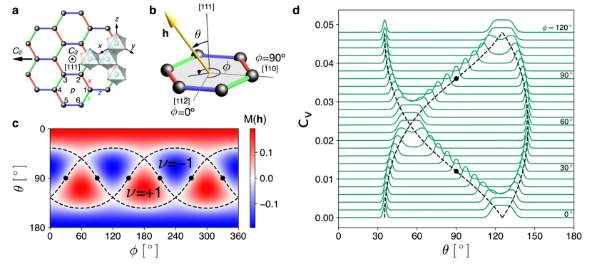
Figure 1: Field angle dependence of the pure Kitaev model. a Honeycomb lattice enclosed by edge-sharing octahedra. Red, green, blue lines denote the $x$,$y$,$z$-bonds, and the six numbers indicate the numbering convention for sites in each hexagon plaquette ($p$). Black arrows depict $C_{3}$ and $C_{2}$ rotation axes. b Convention for the angular representation of an applied magnetic field ${\bf h}$ (yellow). The polar and azimuthal angles ($\theta,\phi$) are measured from the out-of-plane $[111]$ axis and the bond-perpendicular $[11\bar{2}]$ axis, respectively. c Color map of the mass function $M(\mathbf{h})=h_{x}h_{y}h_{z}/K^{2}$ on the ($\theta,\phi$) plane. The dashed lines highlight the topological phase transitions between the $\nu=\pm 1$ states, i.e., the quantum critical lines of the energy gap $\Delta(\mathbf{h})\propto|M(\mathbf{h})|=0$. The black dots mark the bond directions $(\theta=90^{\circ},\phi=30^{\circ}+n\cdot 60^{\circ})$, where $n=0,1,\cdots,5$. d A schematic of the field angle dependence of the heat capacity $c_{v}$ at a fixed temperature, where peak positions determine the critical lines of the non-abelian KQSL.

Results

Model and symmetries. We consider a generic spin-1/2 model on the honeycomb lattice with edge-sharing octahedron crystal structure,

$$H_{KJ\varGamma\varGamma^{\prime}}=\sum_{\langle jk\rangle_{\gamma}} \left[KS_{j}^{\gamma}S_{k}^{\gamma}+J\mathbf{S}_{j}\cdot\mathbf{S}_{k}+\varGamma\big{(}S_{j}^{\alpha}S_{k}^{\beta}+S_{j}^{\beta}S_{k}^{\alpha}\big{)}\right.$$

$$+ \left.\varGamma^{\prime}\big{(}S_{j}^{\alpha}S_{k}^{\gamma}+S_{j}^{\gamma}S_{k}^{\alpha}+S_{j}^{\beta}S_{k}^{\gamma}+S_{j}^{\gamma}S_{k}^{\beta}\big{)}\right],$$

so-called $K$-$J$-$\varGamma$-$\varGamma^{\prime}$ model Rau2014 ; KimHS ; Winter2016 ; Winter2017review . Nearest neighbor bonds of the model are grouped into $x,y,z$-bonds depending on the bond direction (Fig. 1a). Spins ($\mathbf{S}_{j,k}$) at each bond are coupled via the Kitaev ($K$), Heisenberg ($J$), and off-diagonal-symmetric ($\varGamma,\varGamma^{\prime}$) interactions. The index $\gamma\in\{x,y,z\}$ denotes the type of bond, and the other two $\alpha,\beta$ are the remaining components in $\{x,y,z\}$ other than $\gamma$. Under an applied magnetic field (${\bf h}$), the Hamiltonian becomes

$$H(\theta,\phi)=H_{KJ\varGamma\varGamma^{\prime}}-\mathbf{h}(\theta,\phi)\cdot\sum_{j}\mathbf{S}_{j}.$$ (1)

We specify the magnetic field direction with the polar and azimuthal angles $(\theta,\phi)$ as defined in Fig. 1b. $H_{KJ\varGamma\varGamma^{\prime}}$ possesses the symmetries of time reversal, spatial inversion, $C_{3}$ rotation about the normal axis to each hexagon plaquette, and $C_{2}$ rotation about each bond axis (Fig. 1a). The $C_{3}$ and $C_{2}$ rotations form a dihedral group $D_{3}$. Under each of these symmetries, $H(\theta,\phi)$ is transformed to $H(\theta^{\prime},\phi^{\prime})$ with a rotated magnetic field $\mathbf{h}(\theta^{\prime},\phi^{\prime})$; see Supplementary Notes 1 and 2.

In the pure Kitaev model, parton approach provides the exact wave function of KQSL together with gapped $\mathbb{Z}_{2}$ flux and gapless Majorana fermion excitations. Application of magnetic fields drives the KQSL into the non-abelian phase by opening an energy gap in Majorana fermion excitations. The gap size is proportional to the mass function, $M(\mathbf{h})=h_{x}h_{y}h_{z}/K^{2}$, and the topological invariant (Chern number) of the KQSL is given by the sign of the mass function, ${\rm sgn}(h_{x}h_{y}h_{z})$ Kitaev .

Topologically protected critical lines. Topological invariant of non-abelian phases with Majorana fermions can be defined from the quantized thermal Hall conductivity, $\kappa_{xy}/T=\nu(\pi/12)(k_{B}^{2}/\hbar)$, where $\nu$ is the topological invariant representing the total number of chiral Majorana edge modes ($T$: temperature)Kitaev . While the topological invariant in the pure Kitaev model is exactly calculated by the Chern number of Majorana fermions, it is a nontrivial task to analyze the topological invariant for the generic model $H(\theta,\phi)$.

Our strategy to overcome the difficulty is to exploit symmetry properties of the topological invariant and find characteristic features of the non-abelian KQSL. Concretely, we focus on the landscape of $\nu({\bf h})$ on the plane of the magnetic field angles $(\theta,\phi)$. Our major finding is that critical lines of $\nu({\bf h})$ must arise as an intrinsic topological property of the non-abelian KQSL.

We first consider time reversal symmetry and note the following three facts:

• Time reversal operation reverses the topological invariant as $\nu(\mathbf{h})\rightarrow-\nu(\mathbf{h})$.

• Time reversal operation also reverses the magnetic field direction: ${\bf h}(\theta,\phi)\rightarrow-{\bf h}(\theta,\phi)={\bf h}(\pi-\theta,\phi+\pi)$.

• Topologically distinct regions with $\{+\nu(\mathbf{h}),+{\bf h}\}$ and $\{-\nu(\mathbf{h}),-{\bf h}\}$ exist on the $(\theta,\phi)$ plane.

These properties enforce the two regions to meet by hosting critical lines where Majorana fermion excitations become gapless. In other words, topological phase transitions must occur as the field direction changes. We propose that the very existence of critical lines can be used in experiments as an identifier for the KQSL.

We further utilize the $D_{3}$ symmetry of the system. The topological invariant $\nu$ and thermal Hall conductivity $\kappa_{xy}$ are $A_{2}$ representations of the $D_{3}$ group, i.e., even under $C_{3}$ rotations but odd under $C_{2}$ rotations, which reveals the generic form,

$$\nu(\mathbf{h})={\rm sgn}[\Lambda_{1}(h_{x}+h_{y}+h_{z})+\Lambda_{3}h_{x}h_{y}h_{z}],$$ (2)

where $\Lambda_{1,3}$ are field-independent coefficients. The $h$-linear term $(h_{x}+h_{y}+h_{z})$ and $h$-cubic term $(h_{x}h_{y}h_{z})$ are the leading order $A_{2}$ representations of magnetic fields. Conducting third order perturbation theory, we find the coefficients

$$\Lambda_{1}=-\frac{4\varGamma^{\prime}}{\Delta_{\rm flux}}+\frac{6J\varGamma^{\prime}}{\Delta_{\rm flux}^{2}}-\frac{4\varGamma\varGamma^{\prime}}{\Delta_{\rm flux}^{2}}+\frac{5\varGamma^{\prime 2}}{2\Delta_{\rm flux}^{2}}~{}\&~{}\Lambda_{3}=\frac{18}{\Delta_{\rm flux}^{2}},~{}~{}~{}~{}~{}$$ (3)

where $\Delta_{\rm flux}=0.065|K|$ means the flux gap in the Kitaev limit. See Supplementary Notes 3, 4, 5 and Ref. Takikawa2019 for more details of the perturbation theory.

Notice that the $h$-linear term is completely absent in the pure Kitaev model ($\Lambda_{1}=0$). Figure 1c visualizes the topological invariant, $\nu(\mathbf{h})={\rm sgn}(h_{x}h_{y}h_{z})$. The dashed lines highlight the critical lines representing the topological phase transitions between the phases with $\nu(\mathbf{h})=\pm 1$, where the energy gap of Majorana fermion excitations is closed: $\Delta(\mathbf{h})=0$.

Exploiting the symmetry analysis, we stress two universal properties of the KQSL with the $D_{3}$ symmetry.

1. Symmetric zeroes: for bond direction fields, topological transition/gap closing is guaranteed to occur by the symmetry, i.e., $\Delta({\bf h})=0$ for $(\theta=90^{\circ},\phi=30^{\circ}+n\cdot 60^{\circ})$.

2. Cubic dependence: for in-plane fields, the $h$-cubic term governs low field behaviors of the KQSL, e.g., $\nu({\bf h})\sim\textup{sgn}(h_{x}h_{y}h_{z})$ & $\Delta({\bf h})\sim|h_{x}h_{y}h_{z}|$ for $\theta=90^{\circ}$.

The universal properties and critical lines of the KQSL are numerically investigated for the generic Hamiltonian $H(\theta,\phi)$ in the rest of the paper.

Chirality operator. We introduce the chirality operator

$$\hat{\chi}_{p}=S_{2}^{x}S_{1}^{z}S_{6}^{y}+S_{5}^{x}S_{4}^{z}S_{3}^{y}+C_{3}~{}{\rm rotated~{}terms}$$ (4)

at each hexagon plaquette $p$ and investigate the expectation value of the chirality operator, shortly the chirality,

$$\chi(\mathbf{h})\equiv\frac{1}{N}\sum_{p}\langle\Psi_{\rm KQSL}(\mathbf{h})|\hat{\chi}_{p}|\Psi_{\rm KQSL}(\mathbf{h})\rangle,$$ (5)

and its sign,

$$\bar{\nu}(\mathbf{h})\equiv{\rm sgn}[\chi(\mathbf{h})],$$ (6)

where $|\Psi_{\rm KQSL}({\bf h})\rangle$ is the ground state of the full Hamiltonian $H(\theta,\phi)$ in the KQSL phase ($N$ is the number of unit cells). The chirality operator $\hat{\chi}_{p}$ produces the mass term of Majorana fermions and determines the topological invariant in the pure Kitaev limit Kitaev . More precisely, how magnetic fields couple to the chirality operator determines the topological invariant and the Majorana energy gap. The chirality $\chi$ and its sign $\bar{\nu}$ are in the $A_{2}$ representation of the $D_{3}$ group as of the topological invariant ${\nu}$. We note that the relation between the chirality and the Majorana energy gap, $\chi\sim\Delta$, holds near the symmetric zeroes in a generic KQSL beyond the pure Kitaev model due to the symmetry properties (Supplementary Note 6).

Exact diagonalization. The Hamiltonian $H(\theta,\phi)$ is solved via exact diagonalization (ED) on a 24-site cluster with sixfold rotation symmetry and a periodic boundary condition (Fig. 1a). Resulting phase diagrams are provided in the section of Methods. Figures 2 and 3 display our major results, the ED calculations of the chirality $\chi_{\rm ED}({\bf h})$ for the KQSL. The used parameter sets are listed in Table 1. The zero lines [$\chi_{\rm ED}({\bf h})=0$; dashed lines in the figures] exist in all the cases.

The two universal features of the KQSL are well captured by the chirality (Figs. 2 and 3). Firstly, the zero lines of the chirality $\chi_{\rm ED}(\mathbf{h})$ always pass through the bond directions (marked by black dots), i.e., the symmetric zeroes. Secondly, the chirality shows the cubic dependence for in-plane fields ($\theta=90^{\circ}$). The linear term, $h_{x}+h_{y}+h_{z}$, vanishes for in-plane fields, and the cubic term, $h_{x}h_{y}h_{z}$, determines the chirality at low fields, which is confirmed in our ED calculations (lower panels of Fig. 2). Below, we show how non-Kitaev interactions affect topological properties of the non-abelian KQSL.

Case	$K$	$J$	$\varGamma$	$\varGamma^{\prime}$	Phase	Figures
#1	-1	0	0	0	KQSL	2a, 3a
#2	-1	0.05	0	0	KQSL	2b, 3b
#3	-1	0.05	0	0.05	KQSL	2c, 3c
#4	-1	0.08	0.01	0.05	KQSL	2d, 3d
#5	-1	-0.2	-0.2	0.05	FM	4b
#6	-1	0.2	0.05	0.05	Stripy	4c
#7	-1	0.2	-0.2	0.05	Vortex	4d
#8	1	0.2	-0.2	-0.05	Neel	4e
#9	-1	-0.3	1	-0.1	Zigzag	4f

Table 1: Parameter sets for exact diagonalization and spin wave calculations.

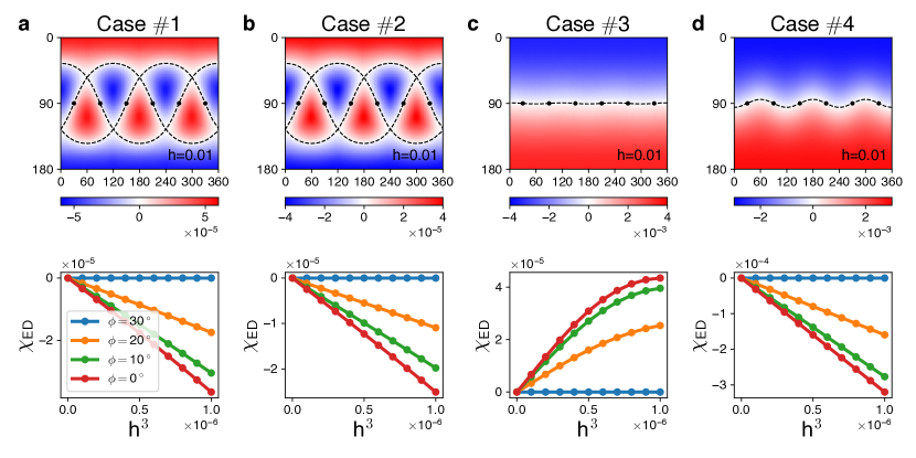
Figure 2: Chirality of the non-abelian KQSL. Upper: color maps of the chirality $\chi_{\rm ED}({\bf h})$ on the plane of the field angles $(\theta,\phi)$, where the magnetic field strength is fixed by $h=0.01$ (horizontal axis: $\phi~{}[^{\circ}]$, vertical axis: $\theta~{}[^{\circ}]$). The dashed lines highlight the zero lines $\chi_{\rm ED}({\bf h})=0$, and the black dots mark the bond directions. Lower: $\chi_{\rm ED}({\bf h})$ as a function of $h^{3}$ for the in-plane fields $(\theta=90^{\circ},\phi=0^{\circ},10^{\circ},20^{\circ},30^{\circ})$, illustrating the universality of the $h^{3}$ behavior in the KQSL. In the case $\#3$, the bending at $h^{3}>0.5\times 10^{-6}$ is an effect of higher order contributions ($h^{5},h^{7},\cdots$). The parameter sets used in the four cases ($\#1\sim 4$) are listed in Table 1.

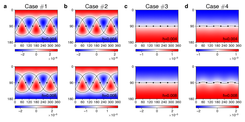
Figure 3: Field evolutions of the zero lines. Color maps of the chirality $\chi_{\rm ED}({\bf h})$ on the plane of the field angles $(\theta,\phi)$ with increasing magnetic field $h=0.004,~{}0.008$ (horizontal axis: $\phi~{}[^{\circ}]$, vertical axis: $\theta~{}[^{\circ}]$). The dashed lines highlight the zero lines $\chi_{\rm ED}({\bf h})=0$, and the black dots mark the bond directions. The parameter sets used in the four cases ($\#1\sim 4$) are listed in Table 1.

Most of all, we find that $\bar{\nu}$ becomes identical to $\nu$ for the pure Kitaev model in Fig. 2a. It is remarkable that the two different methods, ED calculations of the chirality sign and the parton analysis, show the complete agreement: $\bar{\nu}({\bf h})=\nu({\bf h})$. The agreement indicates that the topological phase transitions can be identified by using the chirality operator, which becomes a sanity check of our strategy to employ the chirality operator.

Figure 2b illustrates effects of the Heisenberg interaction ($J$) on the chirality. The shape of the critical lines is unaffected by the Heisenberg interaction, remaining the same as in the pure Kitaev model. This result is completely consistent with the perturbative parton analysis [Eq. (3) and Supplementary Fig. 2b], indicating the validity of our strategy.

Figure 2c-d presents consequences of the other non-Kitaev interactions, $\varGamma^{\prime}$ and $\varGamma$. The zero lines tend to be flatten around the equator $\theta=90^{\circ}$, which can be attributed to the $h$-linear term induced by the non-Kitaev interactions: $h_{x}+h_{y}+h_{z}=h\sqrt{3}\cos\theta$. In other words, the zero lines substantially deviate from those of the pure Kitaev model by the non-Kitaev couplings, $\varGamma^{\prime}$ and $\varGamma$. We point out that the signs of the chirality are opposite to the Chern numbers of the third order perturbation parton analysis (Supplementary Fig. 2c-d). The opposite signs indicate that the two methods have their own valid conditions, calling for improved analysis (Supplementary Note 8).

Impacts of the non-Kitaev interactions also manifest in the field evolution of the zero lines (Fig. 3). Without the non-Kitaev couplings, $\varGamma^{\prime}$ and $\varGamma$, the shape of the critical lines is governed by the cubic term $h_{x}h_{y}h_{z}$, as shown in Fig. 3a-b. In presence of the $\varGamma^{\prime}$ or $\varGamma$ coupling, the $h$-cubic term competes with the $h$-linear term as illustrated in Fig. 3c-d. Namely, the linear term dominates over the cubic term at low fields while the dominance gets reversed at high fields (see Supplementary Note 11 and Supplementary Table 4 for more results). The competing nature may be used to quantitatively characterize the non-Kitaev interactions.

Similarities and differences between the topological invariant, $\nu({\bf h})$, and the sign of the chirality, $\bar{\nu}({\bf h})$, are emphasized. First, the two quantities are identical in the Kitaev limit while they can be generally different by non-Kitaev interactions. Second, the two quantities are in the same representation of the $D_{3}$ group, so $\bar{\nu}({\bf h})$ and $\nu({\bf h})$ have in common the symmetric zeroes. Third, differences between the two quantities may be understood by considering other possible $A_{2}$ representation spin operators that may contribute to the topological invariant. For example, linear and higher-order spin operators exist in addition to the chiral operator. Since the topological invariant $\nu$ is related with the thermal Hall conductivity $\kappa_{xy}$, the associated energy current operator directly informs us of relevant spin operators to the topological invariant. We find that linear spin operator is irrelevant to $\kappa_{xy}$ and $\nu$ (Supplementary Note 7). We also evaluate the expectation values of higher-order spin operators for the KQSL and confirm that their sizes are substantially small compared to the chirality (Supplementary Note 8). Therefore, we argue that the critical lines of the non-abelian KQSL are mainly determined by the zero lines of the chirality.

Discussion

Intrinsic topological properties of the non-abelian KQSL including the critical lines, the symmetric zeroes, and the cubic dependence are highlighted in this work by exploiting the symmetries of time reversal and $D_{3}$ point group. The chirality operator is used to evaluate the topological properties of the KQSL via the ED calculations. Now we discuss how the properties are affected by lattice symmetry breaking such as stacking faults in real materials. First, the existence of the critical lines relies on time reversal, thus it is not destroyed by lattice symmetry breaking. The symmetric zeroes appearing at the bond directions, however, are a consequence of the $D_{3}$ symmetry. The locations of the zeroes get shifted upon breaking the symmetry, which is confirmed in ED calculations of the chirality.

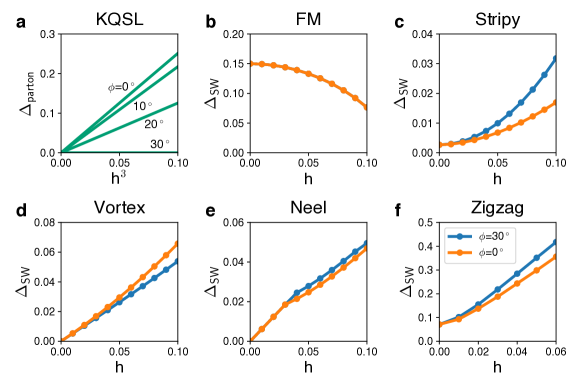
Figure 4: Comparison of the KQSL with magnetically ordered phases. a KQSL: Majorana energy gap $\Delta_{\rm parton}$ as a function of $h^{3}$ for the in-plane fields, $(\theta=90^{\circ},\phi=0^{\circ},10^{\circ},20^{\circ},30^{\circ})$, obtained by a parton theory. b-f Ferromagnetic (FM), stripy, vortex, Neel, and zigzag phases: Magnon gap $\Delta_{\rm SW}$ as a function of $h$ for the in-plane fields, $(\theta=90^{\circ},\phi=0^{\circ},30^{\circ})$, obtained with a spin wave theory for the parameter sets $\#5\sim 9$ in Table 1.

The cubic dependence for in-plane fields also originates from the $D_{3}$ symmetry and topology in the KQSL. The characteristic nonlinear response is not expected in magnetically ordered phases, which we check by performing spin wave calculations. Figure 4 contrasts the KQSL with magnetically ordered phases in terms of excitation energy gap (Majorana gap vs. magnon gap). The magnetic phases show completely different behaviors from the $h$-cubic dependence. Hence, the characteristic cubic dependence under in-plane magnetic fields may serve as an experimentally measurable signature of the KQSL.

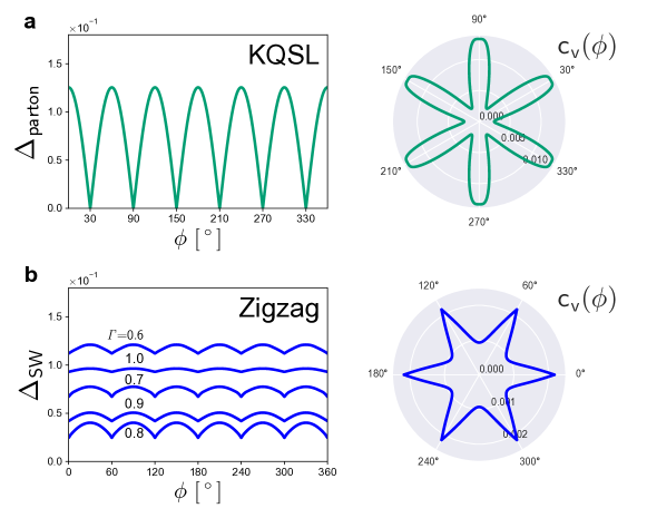
Figure 5: Magnetic field angle dependence of specific heat in the KQSL and zigzag states. a KQSL state: Majorana gap $\Delta_{\rm parton}$ and specific heat $c_{v}$ as functions of in-plane field angle $\phi$, obtained by a parton theory. b Zigzag state: magnon gap $\Delta_{\rm SW}$ and specific heat $c_{v}$ as functions of in-plane field angle $\phi$, obtained by a spin wave theory with $(K,\varGamma,\varGamma^{\prime},h)=(-1,0.8,-0.05,0.03)~{}\&~{}k_{B}T=0.01$. Magnon gaps for other values of $\varGamma$ are shown together to highlight the generality of the field angle dependence.

The universal properties of the KQSL can be observed by heat capacity experiments. Figure 5a illustrates the calculated specific heat $c_{v}(\phi)$ for the KQSL as a function of in-plane field angle $\phi$ (where magnetic field is rotated within the honeycomb plane). The specific heat is maximized by gapless continuum of excitations when the magnetic field is aligned to the bond directions. For comparison, the zigzag state, observed in $\alpha$-RuCl₃ at zero field, is investigated by using a spin wave theory. The magnon spectrum is gapped due to completely broken spin rotation symmetry, so there is no critical line on the $(\theta,\phi)$ plane (Fig. 5b). Compared to the KQSL, the zigzag state exhibits reverted patterns of $\phi$ dependence in the excitation energy gap and specific heat. The energy gap is maximized and the specific heat is minimized at the bond directions. This behavior is closely related with the structure of spin configuration: all spin moments are aligned perpendicular to a certain bond direction selected by magnetic field direction (Supplementary Note 9). The distinct patterns of $\phi$ dependence in Fig. 5 characterize differences between the non-abelian KQSL and zigzag states. Remarkably, such behaviors were observed in the recent heat capacity experiments with in-plane magnetic fields Shibauchi2020specificheat . Covering the polar angle ($\theta$) in the heat capacity measurements will provide more detailed information on the critical lines and spin interactions in $\alpha$-RuCl₃ (see Fig. 1d).

Lastly, we have examined the chirality and critical behaviors of excitation energy gap for magnetically ordered phases of $H(\theta,\phi)$. It is found that the associated magnon gap does not have any critical lines, and there is no resemblance/correlation between the magnon gap and the chirality (Supplementary Note 9).

To summarize, we have uncovered characteristics of the non-abelian Kitaev quantum spin liquid, including the topologically protected critical lines, the symmetric zeroes, and the $h$-cubic dependence for in-plane fields, by using ED calculations with the chirality operator. Furthermore, we characterize the topological fingerprints of the KQSL in heat capacity. We expect our findings to be useful guides for identifying the KQSL in candidate materials such as $\alpha$-RuCl₃. Investigation of the universal properties in field angle dependence of thermodynamic quantities such as spin susceptibility is highly desired, and it would be also useful to apply our results to the recently studied field angle dependence of thermodynamic quantitiesVojta2018 ; Shibauchi2020specificheat ; Modic2018 ; Riedl2019 ; Kee2021 ; Bachus2021 .

Methods

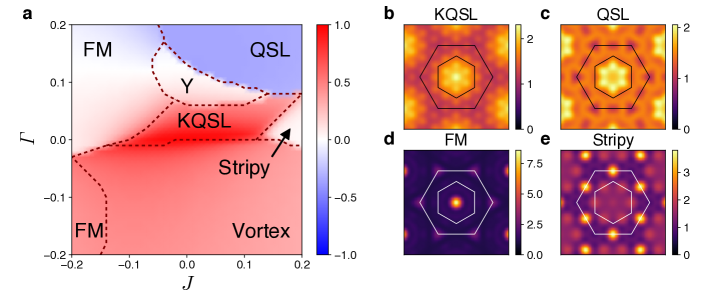
Figure 6: Ferromagnetic KQSL and nearby magnetic states. a Phase diagram of $H_{KJ\varGamma\varGamma^{\prime}}$ at $K=-1$ and $\varGamma^{\prime}=0.05$. The color encodes the flux operator expectation value $\langle\hat{W}_{p}\rangle$, and the dashed lines denote phase boundaries determined by the ground state energy second derivatives $-\partial^{2}E_{\rm gs}/\partial\xi^{2}~{}(\xi=J,\varGamma)$. b-e Color maps of the spin structure factor $S({\bf q})$ for the KQSL, QSL, ferromagnetic (FM), and stripy states. The inner and outer hexagons denote the first and second Brillouin zones of the honeycomb lattice.

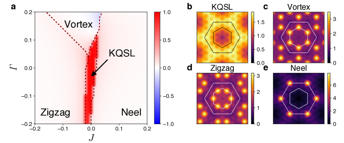
Figure 7: Antiferromagnetic KQSL and adjacent magnetic states. a Phase diagram of $H_{KJ\varGamma\varGamma^{\prime}}$ at $K=1$ and $\varGamma^{\prime}=-0.05$. The color encodes the flux operator expectation value $\langle\hat{W}_{p}\rangle$, and the dashed lines denote phase boundaries determined by the ground state energy second derivatives $-\partial^{2}E_{\rm gs}/\partial\xi^{2}~{}(\xi=J,\varGamma)$. b-e Color maps of the spin structure factor $S({\bf q})$ for the KQSL, vortex, zigzag, and Neel states. The inner and outer hexagons denote the first and second Brillouin zones of the honeycomb lattice.

Exact diagonalization. The KQSL and other magnetic phases of $H(\theta,\phi)$ are mapped out by using the flux operator $\hat{W}_{p}=2^{6}S_{1}^{z}S_{2}^{y}S_{3}^{x}S_{4}^{z}S_{5}^{y}S_{6}^{x}$, the second derivative of the ground state energy $\partial^{2}E_{\rm gs}/\partial\xi^{2}~{}(\xi=J,\varGamma,\varGamma^{\prime})$, and the spin structure factor $S({\bf q})=\frac{1}{N}\sum_{i,j}\langle{\bf S}_{i}\cdot{\bf S}_{j}\rangle e^{i{\bf q}\cdot({\bf r}_{i}-{\bf r}_{j})}$. We find that the KQSL differently responds to non-Kitaev interactions depending on the sign of the Kitaev interaction. Furthermore, the non-abelian phase of the KQSL is ensured by checking topological degeneracy and modular $\mathcal{S}$ matrix Kitaev ; Hickey2019 ; MES_Zhang2012 .

Figures 6 and 7 display the phase diagrams of $H_{KJ\varGamma\varGamma^{\prime}}$. A different structure of phase diagram is found depending on the sign of the Kitaev interaction. With the ferromagnetic Kitaev coupling ($K<0$ as in Fig. 6), the KQSL takes an elongated region along the $J$ axis but substantially narrowed along the $\varGamma$ axis, showing the sensitivity to the $\varGamma$ coupling of the ferromagnetic KQSL. Crossover-type continuous transitions are mostly observed among the KQSL and nearby magnetically ordered states such as ferromagnetic, stripy and vortex states Rau2014 ; Chaloupka2015 ; Chaloupka2019 . Nature of the phase Y is unclarified within the finite size calculation. Unlike the aforementioned magnetically ordered states (Fig. 6d-e), the phase Y does not exhibit sharp peaks and periodicity in the spin structure factor, from which the phase is speculated to have an incommensurate spiral order or no magnetic order. It is remarkable that another quantum spin liquid phase, characterized by negative $\langle\hat{W}_{p}\rangle$, exists in a broad region of the phase diagram (blue region of Fig. 6a) Kee2019 . The QSL and KQSL show similarity in the spin structure factor (Fig. 6b-c). Nonetheless, the QSL as well as the phase Y get suppressed when the sign of $\varGamma^{\prime}$ is changed to negative. A zigzag antiferromagnetic order instead sets in under negative sign of $\varGamma^{\prime}$ (Supplementary Fig. 6).

In case of the antiferromagnetic Kitaev coupling ($K>0$ as in Fig. 7), the KQSL is found to be more sensitive to the Heisenberg coupling rather than the $\varGamma$ coupling, and surrounded by magnetically ordered states such as the vortex, zigzag, and Neel states Rau2014 ; Chaloupka2015 ; Chaloupka2019 . In contrast to the ferromagnetic KQSL case, phase transitions between the antiferromagnetic KQSL and adjacent ordered states are all discontinuous as shown by $\langle\hat{W}_{p}\rangle$ in Fig. 7a. We also find that the antiferromagnetic KQSL and ferromagnetic KQSL are distinguished by different patterns of spin structure factor (Figs. 6b and 7b). Further phase diagrams for other values of $\varGamma^{\prime}$ are provided in Supplementary Fig. 6.

We also examine the phase diagrams at weak magnetic fields, and confirm that the overall structures remain the same as the zero-field results. We find that the chirality is useful for the identification of distinct phase boundaries. In some cases, the chirality performs better than the conventionally used flux (Supplementary Note 12).

We ensure the non-abelian KQSL phase by checking the Ising anyon topological order via threefold topological degeneracy Kitaev ; topo_deg_Kells2009 and modular $\mathcal{S}$ matrix MES_Zhang2012 ; Sheng2014 ; Hickey2019 . As an example, the $\mathcal{S}$ matrix

$$\mathcal{S}_{\rm ED} = \langle\Psi^{\rm MES-I}|\Psi^{\rm MES-II}\rangle$$ (10)

$$= \left[\begin{array}[]{ccc}0.45e^{-i0.08}&0.53e^{-i0.03}&0.70e^{i0.04}\\ 0.53e^{-i0.03}&0.50&-0.71e^{-i0.01}\\ 0.70e^{i0.04}&-0.71e^{-i0.01}&0.02e^{-i2.09}\end{array}\right]$$

$$\approx \left[\begin{array}[]{ccc}1/2&1/2&1/\sqrt{2}\\ 1/2&1/2&-1/\sqrt{2}\\ 1/\sqrt{2}&-1/\sqrt{2}&0\end{array}\right]$$ (14)

is obtained for the parameter set $\#4$ in Table 1 with the magnetic field fixed along the [111] direction ($\theta=0^{\circ}$). See Supplementary Note 10 for the topological degeneracy and modular matrix computation.

Data availability

The data that support the findings of this study are available from the corresponding author on reasonable request.

Code availability

The code used to generate the data in this study is available from the corresponding author upon reasonable request.

Author contributions

E.-G.M. conceived and supervised the project. K.H., J.H.S., and A.G. performed theoretical calculations. K.H. and T.S. contributed to analysis and comparison of theoretical results and experimental data. K.H., A.G., and E.-G.M. prepared the manuscript with the inputs from T.S.

Competing interests

The authors declare no competing interests.

Supplementary Information on “Identification of a Kitaev Quantum Spin Liquid by Magnetic Field Angle Dependence”

Supplementay Note 1 Magnetic field in various coordinate systems

We use two different coordinate systems defined by $\{\hat{x},\hat{y},\hat{z}\}$ and $\{\hat{a},\hat{b},\hat{c}\}$ for magnetic field:

$${\bf h}=h_{x}\hat{x}+h_{y}\hat{y}+h_{z}\hat{z}=h_{a}\hat{a}+h_{b}\hat{b}+h_{c}\hat{c}.$$ (1)

The axes $\{\hat{x},\hat{y},\hat{z}\}$ are the cubic axes of the octahedra enclosing the honeycomb lattice. The other axes $\{\hat{a}\equiv\frac{1}{\sqrt{6}}(\hat{x}+\hat{y}-2\hat{z}),\hat{b}\equiv\frac{1}{\sqrt{2}}(-\hat{x}+\hat{y}),\hat{c}\equiv\frac{1}{\sqrt{3}}(\hat{x}+\hat{y}+\hat{z})\}$ correspond to the bond-perpendicular, bond-parallel, and out-of-plane axes of the honeycomb lattice (Fig. 1a). In the spherical coordinate system ($h,\theta,\phi$), the magnetic field is written as

$$h_{a}=h\sin\theta\cos\phi,~{}h_{b}=h\sin\theta\sin\phi,~{}h_{c}=h\cos\theta,$$ (2)

and

$$h_{x} = h\left(-\frac{1}{\sqrt{2}}\sin\theta\sin\phi+\frac{1}{\sqrt{6}}\sin\theta\cos\phi+\frac{1}{\sqrt{3}}\cos\theta\right),~{}~{}~{}$$ (3)

$$h_{y} = h\left(\frac{1}{\sqrt{2}}\sin\theta\sin\phi+\frac{1}{\sqrt{6}}\sin\theta\cos\phi+\frac{1}{\sqrt{3}}\cos\theta\right),~{}~{}~{}$$ (4)

$$h_{z} = h\left(-\sqrt{\frac{2}{3}}\sin\theta\cos\phi+\frac{1}{\sqrt{3}}\cos\theta\right).~{}~{}~{}$$ (5)

The polar and azimuthal angles ($\theta,\phi$) are measured from the out-of-plane axis $\hat{c}$ and the bond-perpendicular axis $\hat{a}$, respectively (Fig. 1b).

Operation	Field-angle transformation
Time reversal	$H(\theta,\phi)\rightarrow H(180^{\circ}-\theta,180^{\circ}+\phi)$
Spatial Inversion	$H(\theta,\phi)\rightarrow H(\theta,\phi)$
$C_{3}$ rotation	$H(\theta,\phi)\rightarrow H(\theta,120^{\circ}+\phi)$
$C_{2}$ rotation (about $z$-bond)	$H(\theta,\phi)\rightarrow H(180^{\circ}-\theta,180^{\circ}-\phi)$

Supplementary Table 1: Symmetry operations of $H_{JK\varGamma\varGamma^{\prime}}$ and the associated field-angle transformation rules on $H(\theta,\phi)$.

Supplementay Note 2 Symmetry

The symmetries of $H_{JK\varGamma\varGamma^{\prime}}$ are as follows.

• Time reversal : ${\bf S}_{i}\rightarrow-{\bf S}_{i}$.

• Spatial inversion about each bond center of the honeycomb lattice : ${\bf S}_{i}\rightarrow{\bf S}_{i^{\prime}}$.

• $C_{3}$ rotation about the normal axis to each hexagon plaquette : $(S_{i}^{x},S_{i}^{y},S_{i}^{z})\rightarrow(S_{i^{\prime}}^{z},S_{i^{\prime}}^{x},S_{i^{\prime}}^{y})$.

• $C_{2}$ rotation about each bond axis : $(S_{i}^{x},S_{i}^{y},S_{i}^{z})\rightarrow(-S_{i^{\prime}}^{y},-S_{i^{\prime}}^{x},-S_{i^{\prime}}^{z})$ for $z$-bond rotations.

See Fig. 1a for visualizations of the $C_{3}$ and $C_{2}$ rotation axes. Transformation rules of $H(\theta,\phi)$ under the symmetry operations are provided in Supplementary Table 1.

Supplementay Note 3 Coupling between the chirality operator and magnetic field

The full expression of the chirality operator $\chi_{p}$ is given by

$$\hat{\chi}_{p}=S_{2}^{x}S_{1}^{z}S_{6}^{y}+S_{5}^{x}S_{4}^{z}S_{3}^{y}+S_{6}^{z}S_{5}^{y}S_{4}^{x}+S_{3}^{z}S_{2}^{y}S_{1}^{x}+S_{4}^{y}S_{3}^{x}S_{2}^{z}+S_{1}^{y}S_{6}^{x}S_{5}^{z}$$ (6)

with the site convention shown in Fig. 1a.

We determine the most generic coupling form between the chirality operator and magnetic field using symmetry. Suppose we have $f({\bf h})S_{2}^{x}S_{1}^{z}S_{6}^{y}$ at neighboring three sites 2-1-6 in Fig. 1a. Then $f({\bf h})$ should be a polynomial consisting of only odd powers of $h_{x,y,z}$ by time reversal. $C_{2}$ rotation (about the $z$-bond axis passing through the site 1) further constrains $f({\bf h})$ into the form

$$f_{xy,z}({\bf h})$$

$$=\lambda_{1}(h_{x}+h_{y})+\lambda_{2}h_{z}+\lambda_{3}h_{x}h_{y}h_{z}$$

$$+\lambda_{4}(h_{x}^{3}+h_{y}^{3})+\lambda_{5}h_{z}^{3}+\lambda_{6}(h_{x}^{2}h_{y}+h_{x}h_{y}^{2})$$

$$+\lambda_{7}(h_{x}^{2}h_{z}+h_{y}^{2}h_{z})+\lambda_{8}(h_{x}h_{z}^{2}+h_{y}h_{z}^{2})+\mathcal{O}(h^{5}).$$ (7)

Lastly, we apply $C_{3}$ rotation and spatial inversion to $f_{xy,z}({\bf h})S_{2}^{x}S_{1}^{z}S_{6}^{y}$, which generates symmetry-related other five terms at a hexagon plaquette:

$$f_{xy,z}({\bf h})(S_{2}^{x}S_{1}^{z}S_{6}^{y}+S_{5}^{x}S_{4}^{z}S_{3}^{y})+f_{zx,y}({\bf h})(S_{6}^{z}S_{5}^{y}S_{4}^{x}+S_{3}^{z}S_{2}^{y}S_{1}^{x})+f_{yz,x}({\bf h})(S_{4}^{y}S_{3}^{x}S_{2}^{z}+S_{1}^{y}S_{6}^{x}S_{5}^{z}),$$ (8)

where $f_{yz,x}$ and $f_{zx,y}$ are obtained by cyclic permutations of $h_{x,y,z}$ in $f_{xy,z}$. Summing the contributions from all hexagon plaquettes, we arrive at the final expression

$$\sum_{\langle ij\rangle_{\alpha}\langle jk\rangle_{\beta}}f_{\alpha\beta,\gamma}({\bf h})S_{i}^{\alpha}S_{j}^{\gamma}S_{k}^{\beta}.$$ (9)

These effective interactions are generated by applied magnetic fields, and the coupling functions $f_{\alpha\beta,\gamma}({\bf h})$ can be evaluated by the perturbation theory shown below.

Our major finding is summarized before the construction of the perturbation theory. The coupling functions $f_{\alpha\beta,\gamma}({\bf h})$ determine topological properties of the non-abelian Kitaev quantum spin liquid (KQSL). In particular, the chirality is given by

$$\chi=\frac{1}{N}\sum_{p}\langle\hat{\chi}_{p}\rangle\approx-[f_{xy,z}({\bf h})+f_{yz,x}({\bf h})+f_{zx,y}({\bf h})],$$ (10)

and its sign and magnitude are closely related with the Chern number and the energy gap of Majorana fermion excitations. The chirality can be arranged in terms of $A_{2}$ representations of ${\bf h}$:

$$\chi\approx\Lambda_{1}F_{1}+\Lambda_{3}F_{3}+\Lambda^{\prime}_{3}F^{\prime}_{3}+\Lambda^{\prime\prime}_{3}F^{\prime\prime}_{3}+\mathcal{O}(h^{5}),$$ (11)

where the coefficients ($\Lambda$) and the $A_{2}$ representations ($F$) are listed in Supplementary Table 2. The $\Lambda$ coefficients are obtained by the perturbation theory below.

Coefficient	$A_{2}$ representation
$\Lambda_{1}=-(2\lambda_{1}+\lambda_{2})$	$F_{1}({\bf h})=h_{x}+h_{y}+h_{z}$
$\Lambda_{3}=-3\lambda_{3}$	$F_{3}({\bf h})=h_{x}h_{y}h_{z}$
$\Lambda^{\prime}_{3}=-(2\lambda_{4}+\lambda_{5})$	$F^{\prime}_{3}({\bf h})=h_{x}^{3}+h_{y}^{3}+h_{z}^{3}$
$\Lambda^{\prime\prime}_{3}=-(\lambda_{6}+\lambda_{7}+\lambda_{8})$	$F^{\prime\prime}_{3}({\bf h})=h_{x}^{2}h_{y}+h_{x}h_{y}^{2}+h_{y}^{2}h_{z}+h_{y}h_{z}^{2}+h_{z}^{2}h_{x}+h_{z}h_{x}^{2}$

Supplementary Table 2: Expansion of the chirality $\chi$ in terms of $A_{2}$ representations of ${\bf h}$.

Supplementay Note 4 Perturbative expansion

The perturbation theory is developed by decomposing the full Hamiltonian $H$ into the unperturbed part ($H_{0}=\sum_{\langle jk\rangle_{\gamma}}KS_{j}^{\gamma}S_{k}^{\gamma}$) and perturbation part ($H^{\prime}=H-H_{0}$). In this setup, we focus on the zero-flux sector of the pure Kitaev model $H_{0}$ (i.e., $\langle\hat{W}_{p}\rangle=1$).

For a systematic derivation, we employ a quasi-degenerate perturbation theory sref_Winkler2003 and construct an effective Hamiltonian $\mathcal{H}$ in the zero-flux sector. Up to the third order of $H^{\prime}$, the effective Hamiltonian $\mathcal{H}$ is formally given by

$$\mathcal{H}=PH_{0}P-\frac{1}{\Delta_{\textup{flux}}}PH^{\prime}QH^{\prime}P+\frac{1}{\Delta_{\textup{flux}}^{2}}PH^{\prime}QH^{\prime}QH^{\prime}P-\frac{1}{2\Delta_{\textup{flux}}^{2}}(PH^{\prime}PH^{\prime}QH^{\prime}P+{\rm H.c.}),$$ (12)

where $P$ is the projection operator into the zero-flux sector, and $Q=1-P$. Here we have assumed that energy differences between the zero-flux sector and nonzero-flux sectors are simply given by the flux gap $\Delta_{\textup{flux}}(=0.26S^{2}|K|)=0.065|K|$ sref_Kitaev . In order for the perturbation theory to be valid, non-Kitaev couplings should be much smaller than the flux gap ($J,\varGamma,\varGamma^{\prime},h\ll\Delta_{\textup{flux}}$).

The $\lambda$ coefficients in Supplementary Eq. (7) are obtained by the perturbative calculations of Supplementary Eq. (12), which is demonstrated by using the second order term $-\frac{1}{\Delta_{\textup{flux}}}PH^{\prime}QH^{\prime}P$ as an example. Among various interactions generated by the perturbation, we collect components of the chirality operator, $S_{i}^{\alpha}S_{j}^{\gamma}S_{k}^{\beta}$, which are defined over three neighboring sites $ijk$ connected by two bonds $\langle ij\rangle_{\alpha}$ and $\langle jk\rangle_{\beta}$ with all different $\alpha,\beta,\gamma$. This type of terms are produced by $PH^{\prime}QH^{\prime}P$ via two processes: (i) $S_{i}^{\alpha}S_{j}^{\gamma}$ from the $\varGamma^{\prime}$ coupling and $S_{k}^{\beta}$ from the Zeeman coupling, or (ii) $S_{i}^{\alpha}$ from the Zeeman coupling and $S_{j}^{\gamma}S_{k}^{\beta}$ from the $\varGamma^{\prime}$ coupling. These second order processes result in the effective interaction

$$-\frac{1}{\Delta_{\textup{flux}}}PH^{\prime}QH^{\prime}P=P\left[\sum_{\langle ij\rangle_{\alpha}\langle jk\rangle_{\beta}}\frac{2\varGamma^{\prime}(h_{\alpha}+h_{\beta})}{\Delta_{\textup{flux}}}S_{i}^{\alpha}S_{j}^{\gamma}S_{k}^{\beta}\right]P+\cdots$$ (13)

that corresponds to the $\lambda_{1}$ term of Supplementary Eq. (7). Note that the components of the chirality operator appear in the second order because of the presence of $\varGamma^{\prime}$ in drastic contrast to the pure Kitaev model where the chirality operator is generated in the third order sref_Takikawa2019 .

Repeating the perturbative expansion up to the third order, we obtain the effective Hamiltonian

$$\mathcal{H}=P\left[H_{0}+\sum_{\langle ij\rangle_{\alpha}\langle jk\rangle_{\beta}}f_{\alpha\beta,\gamma}({\bf h})S_{i}^{\alpha}S_{j}^{\gamma}S_{k}^{\beta}\right]P+\cdots,$$ (14)

where the $f$ function is given by Supplementary Eq. (7) with the $\lambda$ coefficients:

$$\lambda_{1}=\frac{2\varGamma^{\prime}}{\Delta_{\textup{flux}}}-\frac{5J\varGamma^{\prime}}{2\Delta_{\textup{flux}}^{2}}+\frac{2\varGamma\varGamma^{\prime}}{\Delta_{\textup{flux}}^{2}}-\frac{\varGamma^{\prime 2}}{2\Delta_{\textup{flux}}^{2}},$$ (15)

$$\lambda_{2}=-\frac{J\varGamma^{\prime}}{\Delta_{\textup{flux}}^{2}}-\frac{3\varGamma^{\prime 2}}{2\Delta_{\textup{flux}}^{2}},$$ (16)

$$\lambda_{3}=-\frac{6}{\Delta_{\textup{flux}}^{2}}.$$ (17)

The other coefficients $\lambda_{4,5,6,7,8}$ remain zero ($\lambda_{4,5,6,7,8}=0$) up to third order.

Supplementay Note 5 Parton theory

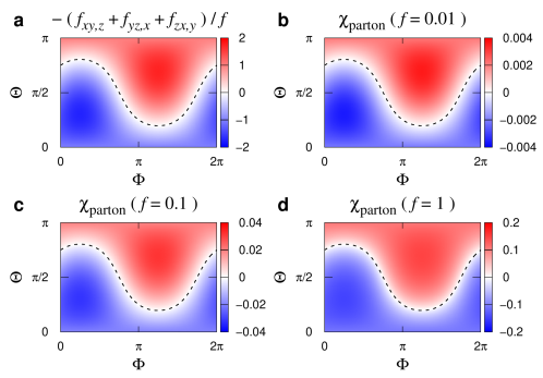
Supplementary Figure 1: Chirality $\bm{\chi_{\rm parton}}$ of the parton theory. a-d Color maps of $-(f_{xy,z}+f_{yz,x}+f_{zx,y})/f$ and $\chi_{\rm parton}$ ($f=0.01,~{}0.1,~{}1$) as functions of $\Theta$ and $\Phi$. In each plot, the dashed line indicates the points of $f_{xy,z}+f_{yz,x}+f_{zx,y}=0$.

Energy gap. The component of the chirality operator $S_{i}^{\alpha}S_{j}^{\gamma}S_{k}^{\beta}$ gives rise to a next-nearest-neighbor hopping term of $c$-Majorana fermions without changing the flux sector sref_Kitaev ; sref_Baskaran2007 . This can be seen from the identity

$$S_{i}^{\alpha}S_{j}^{\gamma}S_{k}^{\beta}=-\frac{i}{8}D_{j}\hat{u}_{ij}\hat{u}_{kj}c_{i}c_{k},$$ (18)

where $\hat{u}_{ij}=ib_{i}^{\alpha}b_{j}^{\alpha}$, $\hat{u}_{kj}=ib_{k}^{\beta}b_{j}^{\beta}$, and $D_{j}=b_{j}^{x}b_{j}^{y}b_{j}^{z}c_{j}$. Applying this to $\mathcal{H}$ in Supplementary Eq. (14), we obtain the effective Majorana Hamiltonian

$$\mathcal{H}=P\left[\sum_{\langle jk\rangle_{\gamma}}\frac{-iK}{4}\hat{u}_{jk}c_{j}c_{k}+\sum_{\langle ij\rangle_{\alpha}\langle jk\rangle_{\beta}}\frac{-if_{\alpha\beta,\gamma}}{8}D_{j}\hat{u}_{ij}\hat{u}_{kj}c_{i}c_{k}\right]P.$$ (19)

For the calculations of fermion excitation spectrum, we choose the uniform configuration of $\mathbb{Z}_{2}$ gauge fields: $\hat{u}_{jk}=1$ for $j\in A$, $k\in B$ (or $\hat{u}_{jk}=-1$ for $j\in B$, $k\in A$), where $A,B$ imply two sublattices of the honeycomb lattice. After the gauge-fixing and Fourier transformation to momentum space, the Hamiltonian is written as

$$\mathcal{H}=\frac{1}{4}\sum_{\bf q}\left[\begin{array}[]{cc}c_{-{\bf q}}^{A}&c_{-{\bf q}}^{B}\end{array}\right]\left[\begin{array}[]{cc}M_{\bf q}&iU_{\bf q}\\ -iU_{\bf q}^{*}&-M_{\bf q}\end{array}\right]\left[\begin{array}[]{c}c_{{\bf q}}^{A}\\ c_{{\bf q}}^{B}\end{array}\right],$$ (20)

where the subscript ${\bf q}$ denotes momentum, and the superscripts $A,B$ imply two sublattices of the honeycomb lattice. The matrix elements are given by $M_{\bf q}=-\frac{1}{2}[f_{xy,z}\sin{\bf q}\cdot({\bf n}_{2}-{\bf n}_{1})+f_{yz,x}\sin{\bf q}\cdot(-{\bf n}_{2})+f_{zx,y}\sin{\bf q}\cdot{\bf n}_{1}],$ and $U_{\bf q}=-\frac{K}{2}(1+e^{i{\bf q}\cdot{\bf n}_{1}}+e^{i{\bf q}\cdot{\bf n}_{2}}),$ where ${\bf n}_{1},~{}{\bf n}_{2}$ imply lattice vectors of the honeycomb lattice. In terms of the complex fermion operators $\Psi_{\bf q}=\left[\psi_{\bf q},\psi_{-{\bf q}}^{\dagger}\right]^{T}\equiv\frac{1}{2}\left[c_{\bf q}^{A}+ic_{\bf q}^{B},c_{\bf q}^{A}-ic_{\bf q}^{B}\right]^{T}$, the Hamiltonian takes the form

$$\mathcal{H}=\frac{1}{2}\sum_{\bf q}\Psi_{\bf q}^{\dagger}~{}{\bf R}({\bf q})\cdot\bm{\sigma}~{}\Psi_{\bf q},$$ (21)

where ${\bf R}({\bf q})=[M_{\bf q},{\rm Im}U_{\bf q},{\rm Re}U_{\bf q}]$ and $\bm{\sigma}=[\sigma_{x},\sigma_{y},\sigma_{z}]$ are the Pauli matrices. Taking a canonical transformation to the quasiparticle basis $\gamma_{\bf q}=u_{\bf q}\psi_{\bf q}+v_{\bf q}\psi_{-{\bf q}}^{\dagger}$, we obtain the diagonalized Hamiltonian $\mathcal{H}=E_{\rm gs}+\sum_{\bf q}\omega_{\bf q}\gamma_{\bf q}^{\dagger}\gamma_{\bf q}$ with the excitation spectrum $\omega_{\bf q}=\sqrt{|M_{\bf q}|^{2}+|U_{\bf q}|^{2}}$ and the ground state energy $E_{\rm gs}=-\frac{1}{2}\sum_{\bf q}\omega_{\bf q}$. The gapless points $\pm{\bf q}_{*}=\pm(\frac{1}{3}{\bf q}_{1}+\frac{2}{3}{\bf q}_{2})$ of the pure Kitaev model are gapped out by the energy gap

$$\Delta_{\rm parton}=\omega_{{\bf q}_{*}} = \frac{\sqrt{3}}{4}|-(f_{xy,z}+f_{yz,x}+f_{zx,y})|,~{}~{}~{}$$ (22)

where ${\bf q}_{1,2}$ are the reciprocal lattice vectors dual to ${\bf n}_{1,2}$.

Chern number. The gapped spin liquid state is topologically characterized by the Chern number sref_Kitaev

$$\nu_{\rm parton}=\int\frac{d^{2}{\bf q}}{4\pi}[\hat{\bf R}\cdot{\partial_{q_{x}}\hat{\bf R}}\times{\partial_{q_{y}}\hat{\bf R}}]={\rm sgn}[-(f_{xy,z}+f_{yz,x}+f_{zx,y})]$$ (23)

which takes either $+1$ or $-1$ depending on the field direction.

Chirality. Finally, we compute the expectation value of the chirality operator $\hat{\chi}$:

$${\chi}_{\rm parton}=\frac{1}{N}\sum_{p}\langle\hat{\chi}_{p}\rangle=\frac{1}{N}\left(\frac{\partial}{\partial f_{xy,z}}+\frac{\partial}{\partial f_{yz,x}}+\frac{\partial}{\partial f_{zx,y}}\right)E_{\rm gs}=-\frac{1}{2N}\sum_{\bf q}\frac{M_{\bf q}L_{\bf q}}{\omega_{\bf q}},$$ (24)

where $N$ is the total number of unit cells, and $L_{\bf q}=-\frac{1}{2}[\sin{\bf q}\cdot({\bf n}_{2}-{\bf n}_{1})+\sin{\bf q}\cdot(-{\bf n}_{2})+\sin{\bf q}\cdot{\bf n}_{1}].$ By conducting numerical computations for ${\chi}_{\rm parton}$, we find the following property:

$$\chi_{\rm parton}=-(f_{xy,z}+f_{yz,x}+f_{zx,y})~{}g,$$ (25)

where $g$ is a positive function of $(f_{xy,z},f_{yz,x},f_{zx,y})$. In the limit of $f=\sqrt{f_{xy,z}^{2}+f_{yz,x}^{2}+f_{zx,y}}\rightarrow 0$, we find that $g\rightarrow 0.21$. Supplementary Fig. 1 illustrates the chirality $\chi_{\rm parton}$ with the parametrization

$$f_{yz,x} = f\sin\Theta\cos\Phi,$$ (26)

$$f_{zx,y} = f\sin\Theta\sin\Phi,$$ (27)

$$f_{xy,z} = f\cos\Theta,$$ (28)

where $f>0$, $\Theta\in[0,\pi]$, and $\Phi\in[0,2\pi]$. On the plane of $\Theta$ and $\Phi$, $\chi_{\rm parton}$ exhibits exactly the same pattern of sign structure as that of $-(f_{xy,z}+f_{yz,x}+f_{zx,y})$; compare Supplementary Fig. 1b-d with a. Therefore, we obtain the relationship

$$\chi_{\rm parton} \propto -(f_{xy,z}+f_{yz,x}+f_{zx,y}).$$ (29)

Notice that the chirality itself is intimately related with the Chern number and the Majorana energy gap: $\nu=\textup{sgn}(\chi)$ and $\Delta\sim|\chi|$.

Combining with the results of Supplementary Eqs. (15)-(17), we obtain the chirality,

$$\chi_{\rm parton}(\mathbf{h})\propto\Lambda_{1}(h_{x}+h_{y}+h_{z})+\Lambda_{3}h_{x}h_{y}h_{z},$$ (30)

the Chern number,

$$\nu_{\rm parton}({\bf h})={\rm sgn}[\Lambda_{1}(h_{x}+h_{y}+h_{z})+\Lambda_{3}h_{x}h_{y}h_{z}],$$ (31)

and the Majorana energy gap,

$$\Delta_{\rm parton}(\mathbf{h})\propto\left|\Lambda_{1}(h_{x}+h_{y}+h_{z})+\Lambda_{3}h_{x}h_{y}h_{z}\right|,$$ (32)

where $\Lambda_{1}=-(2\lambda_{1}+\lambda_{2})$ and $\Lambda_{3}=-3\lambda_{3}$. These results are pictorialized in Supplementary Fig. 2.

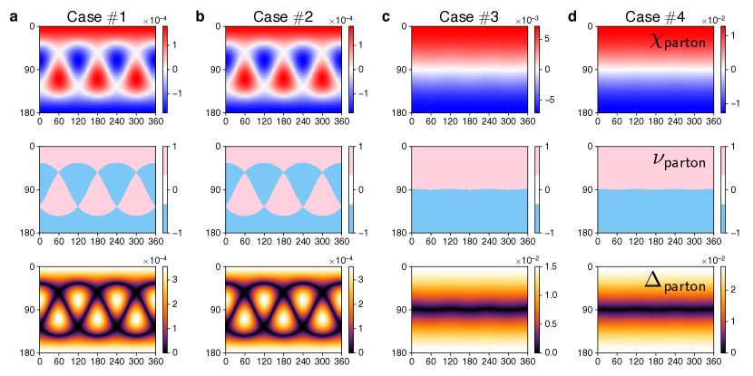
Supplementary Figure 2: Results of the perturbative parton theory. Top, middle, bottom: color maps of the chirality $\chi_{\rm parton}({\bf h})$, the Chern number $\nu_{\rm parton}({\bf h})$, and the Majorana energy gap $\Delta_{\rm parton}({\bf h})$ on the plane of the field angles $(\theta,\phi)$, where the magnetic field strength is fixed by $h=0.01$ (horizontal axis: $\phi~{}[^{\circ}]$, vertical axis: $\theta~{}[^{\circ}]$). The parameter sets used in the four cases ($\#1\sim 4$) are listed in Table 1.

Supplementay Note 6 Relation between the chirality and Majorana gap

The relation, $|\chi|\propto\Delta$, between the chirality and the Majorana energy gap has been established by using the perturbative parton analysis near the pure Kitaev model [Supplementary Eqs. (30,32)]. Here, we provide our reasoning why the relation is expected to hold more generally in our KQSL phase diagrams.

First, we find that the relation $|\chi|\propto\Delta$ holds near the universal zeroes for a generic KQSL with $D_{3}$ symmetry. To show this, let us recall that magnetic fields along the bond directions do not break the bond direction $C_{2}$ symmetry, which makes both $\chi$ and $\Delta$ to be zero. Suppose we slightly tilt the magnetic field from a bond direction by a small angle $\delta\phi~{}(\ll 1)$. The tilting effects appear in the parton Hamiltonian as

$$\left[\begin{array}[]{cc}0&iU_{\bf q}\\ -iU_{\bf q}^{*}&0\end{array}\right]\xrightarrow[]{\text{Tilting the field by}~{}\delta\phi}\left[\begin{array}[]{cc}m\delta\phi&iU_{\bf q}\\ -iU_{\bf q}^{*}&-m\delta\phi\end{array}\right].$$ (33)

It is obvious that Majorana fermions acquire a mass term ($m\delta\phi$), which is an $A_{2}$ representation of the $D_{3}$ symmetry. Then, both of $\chi$ and $\Delta$ are proportional to $\delta\phi$ because they are the same $A_{2}$ representation, and the linear relationship, $|\chi|\propto\Delta$, is thus established near the universal zeroes. We stress that the $D_{3}$ symmetry plays a significant role in our results. In other words, the universal zeroes always appear in a generic KQSL with the $D_{3}$ symmetry, and the relationship must hold in any points of KQSL in our phase diagrams.

Furthermore, we consider another exactly solvable model,

$$H_{\rm\chi}=K\sum_{\langle jk\rangle_{\gamma}}S_{j}^{\gamma}S_{k}^{\gamma}-M\sum_{p}\hat{\chi}_{p},$$ (34)

which consists of the Kitaev interactions ($K$) and the chirality operator three-spin interactions ($M$). The parton analysis shows that the Chern number is $\nu={\rm sgn}(M)$ and the Majorana gap is $\Delta=\frac{3\sqrt{3}}{4}|M|$. Supplementary Fig. 3 presents the calculated chirality $\chi$ as a function of $M$; overall, $\chi$ is proportional to $M$. The positive correlation between $\chi$ and $M$ is demonstrated, establishing the connection between the chirality and the Marjorana gap in a fairly large window ($|M/K|\lesssim 0.5$).

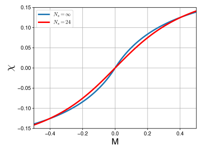
Supplementary Figure 3: Chirality of the model $H_{\rm\chi}$. The chirality $\chi$ as a function of the coupling constant $M$. Red: ED calculation results for the 24-site cluster. Blue: parton analysis results for the infinite system. In all these results, the Kitaev coupling is fixed by $K=-1$.

Supplementay Note 7 Energy current operator

To derive the energy current operator ${\bf J}^{\rm E}$, we arrange the Hamiltonian [Eq. (1)] as

$$H=\sum_{\langle jk\rangle}H_{jk}^{\rm EX}+\sum_{i}H_{i}^{\rm Z},$$ (35)

where $H_{jk}^{\rm EX}$ is the exchange interaction at bond ${\langle jk\rangle}$, and $H_{i}^{\rm Z}$ is the Zeeman coupling at site $i$. Then the energy polarization operator can be written as

$${\bf P}^{\rm E}=\sum_{\langle jk\rangle}\frac{{\bf r}_{j}+{\bf r}_{k}}{2}H_{jk}^{\rm EX}+\sum_{i}{\bf r}_{i}H_{i}^{\rm Z},$$ (36)

where ${\bf r}_{i}$ means the position vector of site $i$. The energy current is nothing but the time derivative of the polarization sref_Han2017 ; sref_Motome2017 :

$${\bf J}^{\rm E}=\frac{d{\bf P}^{\rm E}}{dt}=i[H,{\bf P}^{\rm E}]$$

$$= i\sum_{\langle jk\rangle}\sum_{\langle j^{\prime}k^{\prime}\rangle}\frac{{\bf r}_{j^{\prime}}+{\bf r}_{k^{\prime}}}{2}[H_{jk}^{\rm EX},H_{j^{\prime}k^{\prime}}^{\rm EX}]+i\sum_{i}\sum_{i^{\prime}}{\bf r}_{i^{\prime}}[H_{i}^{\rm Z},H_{i^{\prime}}^{\rm Z}]$$

$$+ i\sum_{\langle jk\rangle}\sum_{i^{\prime}}{\bf r}_{i^{\prime}}[H_{jk}^{\rm EX},H_{i^{\prime}}^{\rm Z}]+i\sum_{i}\sum_{\langle j^{\prime}k^{\prime}\rangle}\frac{{\bf r}_{j^{\prime}}+{\bf r}_{k^{\prime}}}{2}[H_{i}^{\rm Z},H_{j^{\prime}k^{\prime}}^{\rm EX}].$$

In the last equality, the first (second) line shows time reversal odd (even) terms. Interestingly, time reversal odd terms only arise from the commutator $[H_{jk}^{\rm EX},H_{j^{\prime}k^{\prime}}^{\rm EX}]$ because the other commutator is alway zero ($[H_{i}^{\rm Z},H_{i^{\prime}}^{\rm Z}]=0$). As an example, explicit calculations for the Kitaev limit lead to the current operator

$${\bf J}^{\rm E}=\sum_{p}{\bf j}_{p}^{\rm E}$$ (38)

where the local current operator ${\bf j}_{p}^{\rm E}$ at plaquette $p$ is given by

$${\bf j}_{p}^{\rm E} = \frac{K^{2}}{2}({\bf r}_{2}-{\bf r}_{6})S_{2}^{x}S_{1}^{z}S_{6}^{y}+\frac{K^{2}}{2}({\bf r}_{5}-{\bf r}_{3})S_{5}^{x}S_{4}^{z}S_{3}^{y}$$ (39)

$$+ \frac{K^{2}}{2}({\bf r}_{6}-{\bf r}_{4})S_{6}^{z}S_{5}^{y}S_{4}^{x}+\frac{K^{2}}{2}({\bf r}_{3}-{\bf r}_{1})S_{3}^{z}S_{2}^{y}S_{1}^{x}$$

$$+ \frac{K^{2}}{2}({\bf r}_{4}-{\bf r}_{2})S_{4}^{y}S_{3}^{x}S_{2}^{z}+\frac{K^{2}}{2}({\bf r}_{1}-{\bf r}_{5})S_{1}^{y}S_{6}^{x}S_{5}^{z}$$

$$+ (\textup{time reversal even terms}).$$

Notice the appearance of the components of the chirality operator $\hat{\chi}_{p}$ sref_Motome2017 .

Supplementay Note 8 Validity conditions of the perturbative parton theory and chirality operator method

The perturbative parton theory and chirality operator method become exact in the limit of the pure Kitaev model under weak magnetic field. Yet, it is important to note that the two methods have their own validity conditions. It is exceedingly difficult to prove which one is a better approach in general, and additional careful analysis is necessary if the two methods show discrepancy. Below, we discuss the validity conditions of each method as well as how to improve the discrepancy.

Recall that the topological invariant ($\nu$) is determined by the zero temperature limit of thermal hall conductivity over temperature, $\kappa_{xy}/T$. The perturbative parton theory introduces parameters made of non-Kitaev interactions and flux gap such as $\varGamma^{\prime}/\Delta_{{\rm flux}}$, and the topological invariant can be written as the expansion,

$$\nu={\rm sgn}\left[m_{0}+m_{1}\left(\frac{\varGamma^{\prime}}{\Delta_{{\rm flux}}}\right)+m_{2}\left(\frac{\varGamma^{\prime}}{\Delta_{{\rm flux}}}\right)^{2}+\cdots\right].$$

The coefficients $m_{0,1,\cdots}$ are functions of the coupling constants of a given Hamiltonian ($K,J,\varGamma,\varGamma^{\prime},\cdots$). The perturbative parton theory is valid if the parameters such as $\varGamma^{\prime}/\Delta_{{\rm flux}}$ are small enough. The case #2 is expected to be similar to the case #1 as manifested in Fig. 2. For the cases (#3,4), the perturbation parameters are larger, for example $\varGamma^{\prime}/\Delta_{{\rm flux}}=0.77$. Though the perturbative parton theory is powerful, we also note that the convergence of the expansion is neither guaranteed nor proven, especially with multiple coupling constants.

The chirality operator method, on the other hand, is based on a different type of expansions by exploiting symmetry properties. Since $\nu$ is in the time reversal odd $A_{2}$ representation of $D_{3}$ symmetry, we consider the operator associated with $\kappa_{xy}$, commutator/correlator of energy currents as used in Ref. sref_Motome2017 , which can be formally written as

$$\hat{A}_{2}=M_{3}\sum\hat{\chi}_{3}+M_{5}\sum\hat{\chi}_{5}+M_{7}\sum\hat{\chi}_{7}+\cdots.$$

The string operators with an odd number of spin operators connecting two sites on a same sublattice ($\hat{\chi}_{3,5,7}$) are introduced, whose graphical representations are given in Supplementary Fig. 4. Their expectation values ($\langle\hat{\chi}_{3,5,7}\rangle$) determine $\nu$. Note that there is no linear term in the expansion as shown in Supplementary Note 7, and the first term $\sum\hat{\chi}_{3}$ is identical to the chirality operator $\sum_{p}\hat{\chi}_{p}$. The coefficients $M_{3,5,7}$ are functions of the coupling constants of a given Hamiltonian ($K,J,\varGamma,\varGamma^{\prime},\cdots$) while the string operators are independent. The chirality operator method is to truncate the expansion at the leading chirality operator term to determine $\nu$.

The ED calculations with the chirality operator are valid under the conditions,

$$\Big{|}M_{3}\sum\langle\hat{\chi}_{3}\rangle\Big{|}\gg\Big{|}M_{5}\sum\langle\hat{\chi}_{5}\rangle\Big{|},\Big{|}M_{7}\sum\langle\hat{\chi}_{7}\rangle\Big{|},\cdots.~{}~{}~{}$$ (40)

The conditions hold near the pure Kitaev model as manifested in the perfect matches between the ED calculations and the perturbative parton theory for the cases (#1,2). The structure of the chirality operator method can be further analyzed by evaluating the expectation values of $\hat{\chi}_{3,5,7}$ for the cases (#1-4) with a magnetic field along the $[111]$ direction, shown in Supplementary Fig. 4. We find that the cases (#3,4) have hundred times larger values of $|\langle\hat{\chi}_{n}\rangle|$ compared to the cases (#1,2), which are consistent with the larger perturbation parameters of the perturbative parton theory. Moreover, we find that the two ratios,

$$r_{1}\equiv\frac{|\langle\hat{\chi}_{5}\rangle|}{|\langle\hat{\chi}_{3}\rangle|}\sim\frac{1}{10},\quad\quad r_{2}\equiv\frac{|\langle\hat{\chi}_{7}\rangle|}{|\langle\hat{\chi}_{3}\rangle|}\sim\frac{1}{100}$$

for the four cases. Since the chirality operator method works well for the cases (#1,2), the validity conditions [Supplementary Eq. (40)] can be fulfilled if the coefficients $M_{3,5,7}$ of the cases (#3,4) are not much different from the ones of the cases (#1,2).

To check the validity conditions, Supplementary Eq. (40), one needs to calculate the coefficients $M_{3,5,7}$ explicitly. Leaving them for future works, we instead notice that the coefficients $M_{3,5,7}$ are in the trivial representation of the $D_{3}$ symmetry, being functions of energy eigenvalues. We calculate the energy spectrum variances of the lowest hundred energy eigenvalues for the four cases and find that the variances are all less than $5\%$. Thus, it is tempting to assume that $M_{3,5,7,\cdots}$ do not vary much, and then, the ED calculations with the chirality operator would work.

Our proposal with the chirality operator is not only alternative but also complementary to the perturbative parton analysis. Namely, the perfect matches between the two methods’ results for the cases (#1,2) become a sanity check as shown in Fig. 2. If the two methods show discrepancy as in the cases (#3,4), further analysis of the systems are necessary. For the perturbative parton analysis, one obvious way is to perform higher order perturbations. For the chirality operator method, one can try other numerical methods such as density-matrix-renormalization-group (DMRG) calculations since ED calculations with a larger system size are numerically difficult. The topological invariant is believed to be less susceptible to slight symmetry breaking from a cylinder-like lattice shape, and the chirality operator method is expected to be useful even with DMRG calculations.

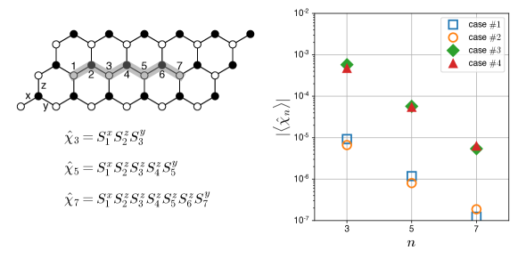
Supplementary Figure 4: Expectation values of the $A_{2}$ operators. Left: pictorial illustration of the operators $\hat{\chi}_{3,5,7}$. Right: the expectation values $\langle\hat{\chi}_{3,5,7}\rangle$ for the four cases #1,2,3,4. The y-axis is in a log scale, and all the results are obtained by 24-site ED calculations with the field $h=0.01\parallel[111]$.

Supplementay Note 9 Spin wave theory

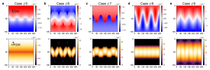
Supplementary Figure 5: Results of the spin wave theory. Upper and bottom: color maps of the chirality $\chi_{\rm SW}({\bf h})$, and the magnon energy gap $\Delta_{\rm SW}({\bf h})$ on the plane of the field angles $(\theta,\phi)$ (horizontal axis: $\phi~{}[^{\circ}]$, vertical axis: $\theta~{}[^{\circ}]$). The parameter sets used in the five cases ($\#5\sim 9$) are listed in Table 1. The magnetic field strength is fixed by $h=0.1$ in the cases $\#5\sim 8$ and $h=0.06$ in the case $\#9$. The black regions in the magnon gap indicate the regions where each magnetic order becomes unstable by magnon condensation.

Magnon gap and chirality. Field angle dependence of magnetically ordered phases are investigated using spin wave theories based on the linearized Holstein-Primakoff spin representation:

$$\begin{array}[]{ccl}{S}^{X}&=&\sqrt{\frac{S}{2}}(a+a^{\dagger}),\\ {S}^{Y}&=&-i\sqrt{\frac{S}{2}}(a-a^{\dagger}),\\ {S}^{Z}&=&S-a^{\dagger}a,\end{array}$$ (41)

where the local axis $Z$ is defined by the classical spin configuration $\{{\bf S}_{i}^{\rm cl}\}$ of the Hamiltonian $H(\theta,\phi)$, and the other two local axes $X,Y$ are perpendicular to the axis $Z$ ($S=1/2$). The boson operator $a$ describes a local spin-flip, essentially the magnon excitation. Applying the linearized representation to the Hamiltonian $H(\theta,\phi)$ leads to the quadratic magnon Hamiltonian

$$\mathcal{H}_{\textup{SW}}=E_{\textup{cl}} + \sum_{\bf k}\sum_{m,n=1}^{N_{\rm s}}A_{mn}({\bf k})~{}a_{m,{\bf k}}^{\dagger}a_{n,{\bf k}}$$ (42)

$$+ \sum_{\bf k}\sum_{m,n=1}^{N_{\rm s}}B_{mn}({\bf k})~{}a_{m,-{\bf k}}a_{n,{\bf k}}+\textup{H.c.}$$

$$+ \sum_{\bf k}\sum_{m=1}^{N_{\rm s}}({\bf h}\cdot{\bf S}_{m}^{\rm cl})a_{m,{\bf k}}^{\dagger}a_{m,{\bf k}},$$

where $E_{\textup{cl}}$ is the energy of the classical spin configuration $\{{\bf S}_{i}^{\rm cl}\}$, ${N_{\rm s}}$ is the number of sites in the magnetic unit cell, the subscripts $m,n$ denote magnetic sublattices, and ${\bf k}$ represents momentum. The hopping amplitude $A_{mn}({\bf k})$ and pairing amplitude $B_{mn}({\bf k})$ are determined by the classical spin configuration. Diagonalizing the magnon Hamiltonian via Bogoliubov transformation, we obtain the magnon energy gap $\Delta_{\rm SW}$ shown in Fig. 4.

For the chirality computation, we simply use the classical spin configuration $\{{\bf S}_{i}^{\rm cl}\}$ since the chirality should be mainly determined by the local spin moments (for magnetically ordered phases). We provide the calculated chirality $\chi_{\rm SW}$ together with the magnon gap $\Delta_{\rm SW}$ in Supplementary Fig. 5.

It is important to note that there is no critical line in the magnon gap. Anisotropic spin interactions of the Kitaev and Gamma terms and the Zeeman coupling break all continuous spin rotational symmetries, so there is no gapless spin excitation. Unlike the KQSL, magnetically ordered phases do not show any resemblance/correlation between the excitation energy gap $\Delta_{\rm SW}$ and the chirality $\chi_{\rm SW}$.

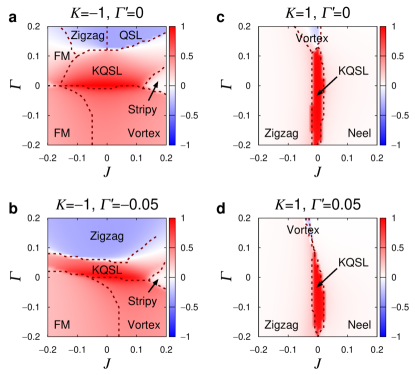
Supplementary Figure 6: $\bm{\varGamma^{\prime}}$ effects on the phases of the $\bm{K}$-$\bm{J}$-$\bm{\varGamma}$-$\bm{\varGamma^{\prime}}$ model.

Zigzag state. Based on the ED results, the zigzag antiferromagnetic state occurs in two distinct parameter regimes. One region is $(K<0,~{}\varGamma>0,~{}\varGamma^{\prime}\leq 0)$ in Supplementary Fig. 6a-b, and the other is $(K>0,~{}J<0)$ as shown in Fig. 7a and Supplementary Fig. 6c-d. We focus on the former case because it is believed to be more relevant to $\alpha$-RuCl₃.

At zero field, the classical ground state manifold of $H_{KJ\varGamma\varGamma^{\prime}}$ is triply degenerate consisting of $x$, $y$, $z$-zigzag states. These three states are related by $C_{3}$ rotation, and the name of each state implies the correlation pattern of spin moments. For instance, in the $z$-zigzag state spin moments are all perpendicular to the $z$-bond axis with being anti-aligned at each $z$-bond.

The degeneracy is lifted when a magnetic field is applied. The degeneracy lift pattern could be understood most intuitively at in-plane fields ($\theta=90^{\circ}$). If the magnetic field is bond-parallel, e.g., aligned to the $z$-bond axis ($\phi=90^{\circ}$), the $z$-zigzag state becomes most stable compared to the other two states. In this case, the field is perpendicular to the spin moments of the $z$-zigzag state, which renders the $z$-zigzag state to develop the largest magnetization amongst the three zigzag states. By a similar mechanism, the $x$-zigzag state is selected near the $x$-bond ($\phi=30^{\circ}$) direction and the $y$-zigzag state is selected near the $y$-bond ($\phi=150^{\circ}$) direction. From this analysis, we gain the insight that the zigzag phase becomes most stable at the bond-parallel field directions $\phi=30^{\circ}+n\cdot 60^{\circ}~{}(n=0,1,2,3,4,5)$. It is corroborated with the largest size of magnon gap $\Delta_{\rm magnon}$ found at the bond-parallel directions (Fig. 5b).

We have checked the same pattern of field angle dependence in the $J$-$K$-$\varGamma$-$J_{3}$ model proposed for $\alpha$-RuCl₃ sref_Winter2017magnon_breakdown ; sref_Winter2018 as well.

Supplementay Note 10 Topological degeneracy and modular matrix

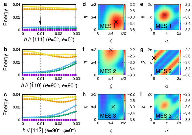
Supplementary Figure 7: Topological degeneracy and entanglement entropy. a-c Evolution of the energy spectrum for three different field directions. d-i Color maps of the entanglement entropy $S_{A}(\zeta,\eta,\alpha,\beta)$ near the states $\{|\Psi_{m}^{\rm MES-I}\rangle\}_{m=1}^{3}$ in Supplementary Table 3. In each map, the entropy is plotted with a reversed sign, $-S_{A}$, which reveals the MES through local maxima. The cross marks denote the location of $|\Psi_{1}^{\rm MES-I}\rangle$ in d-e, $|\Psi_{2}^{\rm MES-I}\rangle$ in f-g, and $|\Psi_{3}^{\rm MES-I}\rangle$ in h-i. All the results are obtained for the case $\#4$ of Table 1, $(K,J,\varGamma,\varGamma^{\prime})=(-1,0.08,0.01,0.05)$, and the computations of entanglement entropy and MES are conducted for the magnetic field $h=0.01\parallel[111]$ (marked by an arrow in a).

MES	$\frac{\zeta}{\pi/2}$	$\frac{\eta}{\pi/2}$	$\frac{\alpha}{2\pi}$	$\frac{\beta}{2\pi}$	$S_{A}$
$|\Psi_{1}^{\rm MES-I}\rangle$	$7/10$	$3/10$	$5/12$	$7/12$	2.22
$|\Psi_{2}^{\rm MES-I}\rangle$	$5/10$	$10/10$	$0/12$	$8/12$	2.36
$|\Psi_{3}^{\rm MES-I}\rangle$	$6/10$	$5/10$	$11/12$	$1/12$	3.15
$|\Psi_{1}^{\rm MES-II}\rangle$	$7/10$	$3/10$	$1/12$	$11/12$	2.22
$|\Psi_{2}^{\rm MES-II}\rangle$	$5/10$	$10/10$	$0/12$	$4/12$	2.36
$|\Psi_{3}^{\rm MES-II}\rangle$	$6/10$	$5/10$	$7/12$	$5/12$	3.15

Supplementary Table 3: Minimally entangled states. The MES are obtained by searching on a $10\times 10\times 12\times 12$ uniform grid of $(\zeta,\eta,\alpha,\beta)$ for the case $\#4$ of Table 1, $(K,J,\varGamma,\varGamma^{\prime})=(-1,0.08,0.01,0.05)~{}~{}\&~{}~{}h=0.01\parallel[111]$.

The non-abelian KQSL state has threefold ground state degeneracy on a torus geometry due to the Ising anyon topological order sref_Kitaev ; sref_topo_deg_Kells2009 . In Supplementary Fig. 7, we demonstrate the degeneracy for a few selected field directions. It is clearly shown that the lowest three states (degeneracy slightly lifted due to the finite size effect) are well separated from the other excited states for small $h$. Furthermore, it is verified that those quasi-degenerate states share qualitatively same bulk properties such as the expectation value of flux operator $\langle\hat{W}_{p}\rangle$, spin structure factor $S({\bf q})$, and also chirality $\chi({\bf h})$.

By using the topological degenerate states, we may extract the modular $\mathcal{S}$ matrix containing the information of quasiparticles’ statistics and fusion rules. It is achieved by finding the so called minimally entangled states (MES) in the subspace of the quasi-degenerate states sref_MES_Zhang2012 ; sref_Sheng2014 :

$$|\Psi\rangle=\sum_{n=1}^{3}z_{n}|\Psi_{n}\rangle,$$ (43)

where $|\Psi_{1,2,3}\rangle$ are the three quasi-degenerate states, and the complex coefficients $z_{1,2,3}$ are parametrized by

$$z_{1} = \sin\zeta\cos\eta,$$ (44)

$$z_{2} = \sin\zeta\sin\eta e^{i\alpha},$$ (45)

$$z_{3} = \cos\zeta e^{i\beta},$$ (46)

with the four angles, $\zeta,\eta\in[0,\pi/2]$ and $\alpha,\beta\in[0,2\pi]$.

To construct the minimally entangled states, we consider two noncontractable bipartitions on the torus geometry (cut I and cut II)  sref_MES_Zhang2012 ; sref_Sheng2014 . Then for each bipartition we compute the entanglement entropy

$$S_{A}=-\log{\rm Tr}\rho_{A}^{2}$$ (47)

where $\rho_{A}$ is the reduced density matrix $\rho_{A}\equiv{\rm Tr}_{B}|\Psi\rangle\langle\Psi|$ traced over the partition $B$ of the torus. The minimally entangled states $\{|\Psi_{n}^{\rm MES}\rangle\}_{n=1}^{3}$ correspond to the local minima of $S_{A}$ in the parameter space of $(\zeta,\eta,\alpha,\beta)$. We list the resulting MES in Supplementary Table 3, and illustrate the entanglement entropy $S_{A}(\zeta,\eta,\alpha,\beta)$ near the MES points in Supplementary Fig. 7d-i. After an appropriate U(1) transformation in each of the MES, the inner products between the two sets of the MES

$$\mathcal{S}_{mn}=\langle\Psi_{m}^{\rm MES-I}|\Psi_{n}^{\rm MES-II}\rangle$$ (48)

yield the modular $\mathcal{S}$ matrix of the Ising topological field theory in Eq. (7).

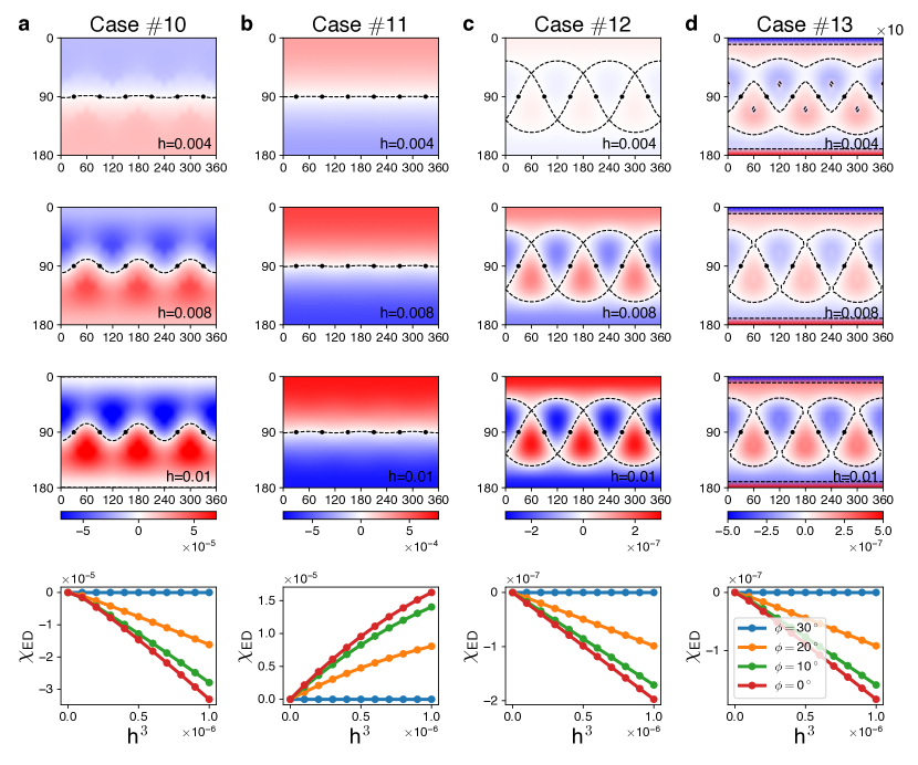
Supplementary Figure 8: Additional results of the chirality for the non-abelian KQSL. Top three: color maps of the chirality $\chi_{\rm ED}({\bf h})$ on the plane of the field angles $(\theta,\phi)$ for the magnetic field strength $h=0.004,~{}0.008,~{}0.01$ (horizontal axis: $\phi~{}[^{\circ}]$, vertical axis: $\theta~{}[^{\circ}]$). The dashed lines highlight the zero lines $\chi_{\rm ED}({\bf h})=0$, and the black dots mark the bond directions. Bottom: $\chi_{\rm ED}({\bf h})$ as a function of $h^{3}$ for the in-plane fields $(\theta=90^{\circ},\phi=0^{\circ},10^{\circ},20^{\circ},30^{\circ})$, illustrating the universality of the $h^{3}$ behavior in the KQSL. The parameter sets used in the four cases ($\#10\sim 13$) are listed in Supplementary Table 4.

Supplementay Note 11 Additional results of the chirality $\chi_{\rm ED}$

Supplementary Fig. 8 presents additional results of the chirality $\chi_{\rm ED}$, obtained for the parameter sets in Supplementary Table 4. The first three cases $\#10\sim 12$ are well understood by the competition between the $h$-linear term $(h_{x}+h_{y}+h_{z})$ and the $h$-cubic term $(h_{x}h_{y}h_{z})$. By contrast, the case $\#13$ shows distinguished field evolution behaviors from the other cases. For instance, high intensity peaks of $\chi_{\rm ED}$ are observed near the two poles $\theta=0^{\circ},~{}180^{\circ}$, enclosed by additional critical lines. These features are attributed to effects of other $h$-cubic terms such as $F^{\prime}_{3}({\bf h})$ and $F^{\prime\prime}_{3}({\bf h})$ in Supplementary Table 2.

The cubic dependence for in-plane fields is confirmed in most of the cases. We find a slight deviation from the cubic dependence in the case $\#10$ near the zero field. To confirm the cubic dependence in ED calculations, it is important to make sure that topological degeneracy is lifted by a small but finite energy gap, eliminating the degeneracy in the ground state (as in Supplementary Fig. 7a-c).

Case	$K$	$J$	$\varGamma$	$\varGamma^{\prime}$	Phase	Supplementary
						figure
#10	-1	0	0	0.0005	KQSL	8a
#11	-1	0	0.01	-0.01	KQSL	8b
#12	1	0	0	0	KQSL	8c
#13	1	0	0.05	0	KQSL	8d

Supplementary Table 4: Additional parameter sets for exact diagonalization.

Supplementay Note 12 Identification of phase boundaries by the chirality

Distinct phase boundaries under magnetic field can be identified clearly by the chirality operator. We demonstrate this by conducting additional ED calculations as shown in Supplementary Fig. 9. We find that the phase boundaries revealed by the plaquette operator ($\hat{W}_{p}$) are equally well captured by the chirality operator ($\hat{\chi}_{p}$). In some cases, the chirality operator works better than the plaquette operator as shown in Supplementary Fig. 9b,e (marked by arrows). This shows that the chirality is also useful for the identification of distinct phase boundaries of the Kitaev system.

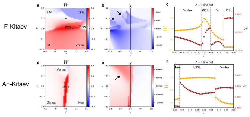
Supplementary Figure 9: Distinct phase boundaries in the chirality. a-c ED results for $K=-1$, $\varGamma^{\prime}=0.05$, $h=0.01\parallel[111]$ with the flux $W~{}(=\langle\hat{W}_{p}\rangle)$, the chirality $\chi~{}(=\langle\hat{\chi}_{p}\rangle)$, and a comparison of $W$ and $\chi$ along the $J=0$ line cut. d-f ED results for $K=1$, $\varGamma^{\prime}=-0.05$, $h=0.01\parallel[111]$ with the flux $W$, the chirality $\chi$, and a comparison of $W$ and $\chi$ along the $J=0$ line cut.

References

- (1) Zhou, Y., Kanoda, K. & Ng, T.-K. Quantum spin liquid states. Rev. Mod. Phys. 89, 025003 (2017).
- (2) Savary, L. & Balents, L. Quantum spin liquids: a review. Rep. Prog. Phys. 80, 016502 (2017).
- (3) Knolle, J. & Moessner, R. A field guide to spin liquids. Annu. Rev. Condens. Matter Phys. 10, 451–472 (2019).
- (4) Sachdev, S. Quantum Phase Transitions (Cambridge University Press, Cambridge, 2011), 2nd edn.
- (5) Wen, X. G. Quantum Field Theory of Many-Body Systems (Oxford University Press, Oxford, 2004).
- (6) Kitaev, A. Anyons in an exactly solved model and beyond. Ann. Phys. (Amsterdam) 321, 2 (2006).
- (7) Jackeli, G. & Khaliullin, G. Mott Insulators in the Strong Spin-Orbit Coupling Limit: From Heisenberg to a Quantum Compass and Kitaev Models. Phys. Rev. Lett. 102, 017205 (2009).
- (8) Chaloupka, J., Jackeli, G. & Khaliullin, G. Kitaev-Heisenberg Model on a Honeycomb Lattice: Possible Exotic Phases in Iridium Oxides . Phys. Rev. Lett. 105, 027204 (2010).
- (9) Chaloupka, J., Jackeli, G. & Khaliullin, G. Zigzag Magnetic Order in the Iridium Oxide . Phys. Rev. Lett. 110, 097204 (2013).
- (10) Rau, J. G., Lee, E. K.-H. & Kee, H.-Y. Generic spin model for the honeycomb iridates beyond the Kitaev limit. Phys. Rev. Lett. 112, 077204 (2014).
- (11) Kim, H.-S., Shankar V., V., Catuneanu, A. & Kee, H.-Y. Kitaev magnetism in honeycomb with intermediate spin-orbit coupling. Phys. Rev. B 91, 241110(R) (2015).
- (12) Kim, H.-S. & Kee, H.-Y. Crystal structure and magnetism in -RuCl3: An ab initio study. Phys. Rev. B 93, 155143 (2016).
- (13) Winter, S. M., Li, Y., Jeschke, H. O. & Valentí, R. Challenges in design of Kitaev materials: Magnetic interactions from competing energy scales. Phys. Rev. B 93, 214431 (2016).
- (14) Rau, J. G., Lee, E. K.-H. & Kee, H.-Y. Spin-orbit physics giving rise to novel phases in correlated systems: Iridates and related materials. Annu. Rev. Condens. Matter Phys. 7, 195–221 (2016).
- (15) Trebst, S. Kitaev materials. Preprint at https://arxiv.org/abs/1701.07056 (2017).
- (16) Winter, S. M. et al. Models and materials for generalized Kitaev magnetism. J. Phys.: Condens. Matter 29, 493002 (2017).
- (17) Baskaran, G., Mandal, S. & Shankar, R. Exact results for spin dynamics and fractionalization in the Kitaev model. Phys. Rev. Lett. 98, 247201 (2007).
- (18) Knolle, J., Kovrizhin, D. L., Chalker, J. T. & Moessner, R. Dynamics of a two-dimensional quantum spin liquid: Signatures of emergent Majorana fermions and fluxes. Phys. Rev. Lett. 112, 207203 (2014).
- (19) Rousochatzakis, I., Reuther, J., Thomale, R., Rachel, S. & Perkins, N. B. Phase diagram and quantum order by disorder in the Kitaev honeycomb magnet. Phys. Rev. X 5, 041035 (2015).
- (20) Chaloupka, J. & Khaliullin, G. Hidden symmetries of the extended Kitaev-Heisenberg model: Implications for the honeycomb-lattice iridates A2IrO3. Phys. Rev. B 92, 024413 (2015).
- (21) Nasu, J., Udagawa, M. & Motome, Y. Thermal fractionalization of quantum spins in a Kitaev model: Temperature-linear specific heat and coherent transport of Majorana fermions. Phys. Rev. B 92, 115122 (2015).
- (22) Song, X.-Y., You, Y.-Z. & Balents, L. Low-energy spin dynamics of the honeycomb spin liquid beyond the Kitaev limit. Phys. Rev. Lett. 117, 037209 (2016).
- (23) Nasu, J., Knolle, J., Kovrizhin, D. L., Motome, Y. & Moessner, R. Fermionic response from fractionalization in an insulating two-dimensional magnet. Nat. Phys. 12, 912 (2016).
- (24) Halász, G. B., Perkins, N. B. & van den Brink, J. Resonant inelastic X-ray scattering response of the Kitaev honeycomb model. Phys. Rev. Lett. 117, 127203 (2016).
- (25) Nasu, J., Yoshitake, J. & Motome, Y. Thermal transport in the Kitaev model. Phys. Rev. Lett. 119, 127204 (2017).
- (26) Winter, S. M. et al. Breakdown of magnons in a strongly spin-orbital coupled magnet. Nat. Commun. 8, 1152 (2017).
- (27) Catuneanu, A., Yamaji, Y., Wachtel, G., Kim, Y. B. & Kee, H.-Y. Path to stable quantum spin liquids in spin-orbit coupled correlated materials. npj Quantum Mater. 3, 23 (2018).
- (28) Gohlke, M., Wachtel, G., Yamaji, Y., Pollmann, F. & Kim, Y. B. Quantum spin liquid signatures in Kitaev-like frustrated magnets. Phys. Rev. B 97, 075126 (2018).
- (29) Lee, H.-Y., Kaneko, R., Okubo, T. & Kawashima, N. Gapless Kitaev spin liquid to classical string gas through tensor networks. Phys. Rev. Lett. 123, 087203 (2019).
- (30) Zhang, S.-S., Wang, Z., Halász, G. B. & Batista, C. D. Vison crystals in an extended Kitaev model on the honeycomb lattice. Phys. Rev. Lett. 123, 057201 (2019).
- (31) Yadav, R. et al. Kitaev exchange and field-induced quantum spin-liquid states in honeycomb -RuCl3. Sci. Rep. 6, 37925 (2016).
- (32) Janssen, L., Andrade, E. C. & Vojta, M. Honeycomb-lattice Heisenberg-Kitaev model in a magnetic field: Spin canting, metamagnetism, and vortex crystals. Phys. Rev. Lett. 117, 277202 (2016).
- (33) Gohlke, M., Verresen, R., Moessner, R. & Pollmann, F. Dynamics of the Kitaev-Heisenberg model. Phys. Rev. Lett. 119, 157203 (2017).
- (34) Gohlke, M., Moessner, R. & Pollmann, F. Dynamical and topological properties of the Kitaev model in a [111] magnetic field. Phys. Rev. B 98, 014418 (2018).
- (35) Zhu, Z., Kimchi, I., Sheng, D. N. & Fu, L. Robust non-abelian spin liquid and a possible intermediate phase in the antiferromagnetic Kitaev model with magnetic field. Phys. Rev. B 97, 241110(R) (2018).
- (36) Winter, S. M., Riedl, K., Kaib, D., Coldea, R. & Valentí, R. Probing -RuCl3 beyond magnetic order: Effects of temperature and magnetic field. Phys. Rev. Lett. 120, 077203 (2018).
- (37) Ye, M., Halász, G. B., Savary, L. & Balents, L. Quantization of the thermal Hall conductivity at small Hall angles. Phys. Rev. Lett. 121, 147201 (2018).
- (38) Hickey, C. & Trebst, S. Emergence of a field-driven U(1) spin liquid in the Kitaev honeycomb model. Nat. Commun. 10, 530 (2019).
- (39) Gordon, J. S., Catuneanu, A., Sørensen, E. S. & Kee, H.-Y. Theory of the field-revealed Kitaev spin liquid. Nat. Commun. 10, 2470 (2019).
- (40) Ronquillo, D. C., Vengal, A. & Trivedi, N. Signatures of magnetic-field-driven quantum phase transitions in the entanglement entropy and spin dynamics of the Kitaev honeycomb model. Phys. Rev. B 99, 140413 (2019).
- (41) Patel, N. D. & Trivedi, N. Magnetic field-induced intermediate quantum spin liquid with a spinon fermi surface. Proc. Natl. Acad. Sci. U.S.A. 116, 12199 (2019).
- (42) Janssen, L. & Vojta, M. Heisenberg-Kitaev physics in magnetic fields. J. Phys.: Condens. Matter 31, 423002 (2019).
- (43) Rusnačko, J., Gotfryd, D. & Chaloupka, J. Kitaev-like honeycomb magnets: Global phase behavior and emergent effective models. Phys. Rev. B 99, 064425 (2019).
- (44) Takagi, H., Takayama, T., Jackeli, G., Khaliullin, G. & Nagler, S. E. Concept and realization of Kitaev quantum spin liquids. Nat. Rev. Phys. 1, 264–280 (2019).
- (45) Motome, Y. & Nasu, J. Hunting Majorana fermions in Kitaev magnets. J. Phys. Soc. Jpn. 89, 012002 (2020).
- (46) Chern, L. E., Kaneko, R., Lee, H.-Y. & Kim, Y. B. Magnetic field induced competing phases in spin-orbital entangled Kitaev magnets. Phys. Rev. Research 2, 013014 (2020).
- (47) Wang, J., Normand, B. & Liu, Z.-X. One proximate Kitaev spin liquid in the -- model on the honeycomb lattice. Phys. Rev. Lett. 123, 197201 (2019).
- (48) Wang, J., Zhao, Q., Wang, X. & Liu, Z.-X. Multinode quantum spin liquids on the honeycomb lattice. Phys. Rev. B 102, 144427 (2020).
- (49) Plumb, K. W. et al. -RuCl3: A spin-orbit assisted Mott insulator on a honeycomb lattice. Phys. Rev. B 90, 041112(R) (2014).
- (50) Sears, J. A. et al. Magnetic order in -RuCl3: A honeycomb-lattice quantum magnet with strong spin-orbit coupling. Phys. Rev. B 91, 144420 (2015).
- (51) Sandilands, L. J., Tian, Y., Plumb, K. W., Kim, Y.-J. & Burch, K. S. Scattering continuum and possible fractionalized excitations in -RuCl3. Phys. Rev. Lett. 114, 147201 (2015).
- (52) Banerjee, A. et al. Proximate Kitaev quantum spin liquid behaviour in a honeycomb magnet. Nat. Mater. 15, 733 (2016).
- (53) Banerjee, A. et al. Neutron scattering in the proximate quantum spin liquid -RuCl3. Science 356, 1055 (2017).
- (54) Do, S.-H. et al. Majorana fermions in the Kitaev quantum spin system -RuCl3. Nat. Phys. 13, 1079 (2017).
- (55) Baek, S.-H. et al. Evidence for a field-induced quantum spin liquid in -RuCl3. Phys. Rev. Lett. 119, 037201 (2017).
- (56) Wolter, A. U. B. et al. Field-induced quantum criticality in the Kitaev system -RuCl3. Phys. Rev. B 96, 041405(R) (2017).
- (57) Leahy, I. A. et al. Anomalous thermal conductivity and magnetic torque response in the honeycomb magnet -RuCl3. Phys. Rev. Lett. 118, 187203 (2017).
- (58) Kasahara, Y. et al. Unusual thermal Hall effect in a Kitaev spin liquid candidate -RuCl3. Phys. Rev. Lett. 120, 217205 (2018).
- (59) Janša, N. et al. Observation of two types of fractional excitation in the Kitaev honeycomb magnet. Nat. Phys. 14, 786 (2018).
- (60) Kasahara, Y. et al. Majorana quantization and half-integer thermal quantum Hall effect in a Kitaev spin liquid. Nature (London) 559, 227 (2018).
- (61) Balz, C. et al. Field-induced intermediate ordered phase and anisotropic interlayer interactions in -RuCl3. Phys. Rev. B 103, 174417 (2021).
- (62) Wulferding, D., Choi, Y., Do, S.H. et al. Magnon bound states versus anyonic Majorana excitations in the Kitaev honeycomb magnet -RuCl3. Nat. Commun. 11, 1603 (2020).
- (63) Yokoi, T. et al. Half-integer quantized anomalous thermal Hall effect in the Kitaev material -RuCl3. Science 373, 568 (2021).
- (64) Yamashita, M., Gouchi, J., Uwatoko, Y., Kurita, N. & Tanaka, H. Sample dependence of half-integer quantized thermal Hall effect in the Kitaev spin-liquid candidate -RuCl3. Phys. Rev. B 102, 220404 (2020).
- (65) Tanaka, O. et al. Thermodynamic evidence for field-angle dependent Majorana gap in a Kitaev spin liquid. Nat. Phys. https://doi.org/10.1038/s41567-021-01488-6 (2022).
- (66) Go, A., Jung, J. & Moon, E.-G. Vestiges of topological phase transitions in Kitaev quantum spin liquids. Phys. Rev. Lett. 122, 147203 (2019).
- (67) Takikawa, D. & Fujimoto, S. Impact of off-diagonal exchange interactions on the Kitaev spin-liquid state of -RuCl3. Phys. Rev. B 99, 224409 (2019).
- (68) Zhang, Y., Grover, T., Turner, A., Oshikawa, M. & Vishwanath, A. Quasiparticle statistics and braiding from ground-state entanglement. Phys. Rev. B 85, 235151 (2012).
- (69) Kells, G., Slingerland, J. K. & Vala, J. Description of Kitaev’s honeycomb model with toric-code stabilizers. Phys. Rev. B 80, 125415 (2009).
- (70) Zhu, W., Gong, S. S., Haldane, F. D. M. & Sheng, D. N. Identifying non-abelian topological order through minimal entangled states. Phys. Rev. Lett. 112, 096803 (2014).
- (71) Modic, K. A. et al. Resonant torsion magnetometry in anisotropic quantum materials. Nat. Commun. 9, 3975 (2018).
- (72) Riedl, K., Li, Y., Winter, S. M. & Valentí, R. Sawtooth Torque in Anisotropic Magnets: Application to -RuCl3. Phys. Rev. Lett. 122, 197202 (2019).
- (73) Gordon, J. S. & Kee, H.-Y., Testing topological phase transitions in Kitaev materials under in-plane magnetic fields: Application to -RuCl3. Phys. Rev. Research 3, 013179 (2021).
- (74) Bachus, S. et al. Angle-dependent thermodynamics of -RuCl3. Phys. Rev. B 103, 054440 (2021).
Acknowledgements
We thank L. Balents, J. H. Han, Y. B. Kim, and Y. Matsuda for invaluable discussions. We also thank B. H. Kim and H.-Y. Lee for useful discussions at the early stage of the project. This work was supported by Institute for Basic Science under Grants No. IBS-R024-D1 (AG), Korea Institute for Advanced Study under Grant No. PG071401 & PG071402 (KH), and NRF of Korea under Grant NRF-2021R1C1C1010429 (AG), NRF-2019M3E4A1080411, NRF-2020R1A4A3079707, and NRF-2021R1A2C4001847 (EGM). Work in Japan was supported by a Grant-in-Aid for Scientific Research on innovative areas “Quantum Liquid Crystals” (JP19H05824) from Japan Society for the Promotion of Science (JSPS), and by JST CREST (JPMJCR19T5). We thank Center for Advanced Computation (CAC) at Korea Institute for Advanced Study (KIAS) for providing computing resources for this work.

References

- (1) Winkler, R., Papadakis, S., De Poortere, E. & Shayegan, M. Spin-Orbit Coupling in Two-Dimensional Electron and Hole Systems, vol. 41 (Springer, 2003).
- (2) Kitaev, A. Anyons in an exactly solved model and beyond. Ann. Phys. (Amsterdam) 321, 2 (2006).
- (3) Takikawa, D. & Fujimoto, S. Impact of off-diagonal exchange interactions on the Kitaev spin-liquid state of -RuCl3. Phys. Rev. B 99, 224409 (2019).
- (4) Baskaran, G., Mandal, S. & Shankar, R. Exact results for spin dynamics and fractionalization in the Kitaev model. Phys. Rev. Lett. 98, 247201 (2007).
- (5) Han, J. H. & Lee, H. Spin chirality and Hall-like transport phenomena of spin excitations. J. Phys. Soc. Jpn. 86, 011007 (2017).
- (6) Nasu, J., Yoshitake, J. & Motome, Y. Thermal transport in the Kitaev model. Phys. Rev. Lett. 119, 127204 (2017).
- (7) Winter, S. M. et al. Breakdown of magnons in a strongly spin-orbital coupled magnet. Nat. Commun. 8, 1152 (2017).
- (8) Winter, S. M., Riedl, K., Kaib, D., Coldea, R. & Valentí, R. Probing -RuCl3 beyond magnetic order: Effects of temperature and magnetic field. Phys. Rev. Lett. 120, 077203 (2018).
- (9) Kells, G., Slingerland, J. K. & Vala, J. Description of kitaev’s honeycomb model with toric-code stabilizers. Phys. Rev. B 80, 125415 (2009).
- (10) Zhang, Y., Grover, T., Turner, A., Oshikawa, M. & Vishwanath, A. Quasiparticle statistics and braiding from ground-state entanglement. Phys. Rev. B 85, 235151 (2012).
- (11) Zhu, W., Gong, S. S., Haldane, F. D. M. & Sheng, D. N. Identifying non-abelian topological order through minimal entangled states. Phys. Rev. Lett. 112, 096803 (2014).