School of Natural Sciences, Institute for Advanced Study,
Princeton, NJ 08540, USA
Following our earlier analyses of nonstandard continuum quantum field theories, we study here gapped systems in dimensions, which exhibit fractonic behavior. In particular, we present three dual field theory descriptions of the low-energy physics of the X-cube model. A key aspect of our constructions is the use of discontinuous fields in the continuum field theory. Spacetime is continuous, but the fields are not.
1 Introduction
The many diverse applications of quantum field theory make its general study interesting in its own right. Our investigation here was motivated by certain lattice systems. In this context continuum quantum field theory gives a universal description of the long-distance physics. As such, it is insensitive to most of the specific details of the microscopic model and therefore it captures its more generic aspects.
This paper is the third in a series of three papers (the earlier ones are [1] and [2]) exploring subtle continuum quantum field theories. (A followup paper [3] explores additional models.) This exploration was motivated by the recent exciting discovery of fractons (for reviews, see e.g. [4, 5] and references therein), which exhibit phenomena that appear to be outside the scope of standard continuum quantum field theory.
Our continuum quantum field theories go beyond the standard framework in three ways:
-
•
Not only are these quantum fields theories not Lorentz invariant, they are also not rotational invariant. The continuum limit is translation invariant, but it preserves only the finite rotation group of the underlying lattice. In [2] and in this paper only the subgroup of the rotations is preserved. This is the group generated by degree rotations. The representations of this group are reviewed in Appendix A.
-
•
As started in the analysis of such systems in [6] and continued in [1, 2], the organizing principle of the discussion is the global symmetries of these systems. We refer to these symmetries, which are quite different than ordinary global symmetries, as exotic global symmetries. The discussion in [2] analyzed many such exotic symmetries and focused on four special ones. We review them in Appendix B and summarize them in Table 1.111As in [1, 2], we limit ourselves to flat spacetime. Space will be mostly a rectangular three-torus . The signature will be either Lorentzian or Euclidean. And when it is Euclidean we will also consider the case of a rectangular four-torus . We will use with or to denote the three spatial coordinates, or for Lorentzian time, and for Euclidean time. When space is a three-torus, the lengths of its three sides will be denoted by . When we take an underlying lattice into account the number of sites in the three directions are , where is the lattice spacing.
-
•
The most significant departure from standard continuum quantum field theory is the use of discontinuous fields. The underlying spacetime is continuous, but we allow certain discontinuous field configurations. A crucial part of the analysis is the precise characterization of the allowed discontinuities. Since we discuss also gauge theories, we should pay attention to the allowed discontinuities in the gauge parameters, which determine the transition functions and the allowed twisted bundles.
All the systems in [1, 2] and here are natural in the sense that they include all low derivative terms that respect their specified global symmetries. However, an important point, which was stressed in [1, 2], is that in these exotic systems, the notions of naturalness and universality are subtle.222We thank P. Gorantla and H.T. Lam for useful discussions about these points. Since we allow some discontinuous field configurations, the expansion in powers of derivatives might not be valid, and certain higher-derivative terms can be as significant as low-derivative terms. As a result, computations using the minimal Lagrangian might not lead to universal results.
A related issue is that of robustness. Most of the systems in [1, 2] are not robust. By that we mean that the low-energy theory includes relevant operators violating the global symmetry. Therefore, small changes in the short-distance physics deform the long-distance theory by these relevant operators. This ruins the elaborate long-distance physics of the system. (See [1] for a review of the role of naturalness and robustness in quantum field theory.)
However, it is important that all the models in this paper are both natural and robust. The low-energy theory does not have any local operators at all. This means that it does not have higher derivative operators that can ruin the universality and it does not have symmetry violating operators that can ruin its robustness. Therefore, small changes of the short-distance physics, including changes that break explicitly the global symmetry, cannot change the long-distance physics.
In [2] we studied four theories. Two of them are non-gauge theories, the -theory and the -theory. The dynamical field is invariant under rotations, while is in the two dimensional representation of the cubic group. Each of these theories has its own momentum and winding symmetries. The -theory has a dipole momentum symmetry and a dipole winding symmetry (see Table 2). The -theory has a momentum tensor symmetry and a winding tensor symmetry (see Table 3).
Then we studied two gauge theories. The gauge symmetry of the -theory is the momentum global symmetry of the -theory, i.e. it is a dipole symmetry. And the gauge symmetry of the -theory is the momentum global symmetry of the -theory, i.e. it is a tensor symmetry. Some aspects of the -theory had been discussed in [7, 8, 9, 10, 11, 12] (see [13, 14, 15, 16, 17, 18, 19, 20, 21, 22, 23, 24, 25, 26, 27, 28] for related tensor gauge theories). And some aspects of the -gauge theory had been discussed in [8]. In the absence of charged matter fields, these gauge theories have their own electric and magnetic global symmetries, which are similar to the electric and magnetic one-form global symmetries of ordinary -dimensional gauge theories [29]. See Table 2 and Table 3.
Surprisingly, the -theory turns out to be dual to the -theory and the -theory turns out to be dual to the -theory. In every one of these dual pairs the global symmetries and the spectra match across the duality. See Table 2 and Table 3. This is particularly surprising given the subtle nature of the states that are charged under the momentum and winding symmetries of the non-gauge systems and states that are charged under the magnetic and electric symmetries of the gauge systems.
Outline
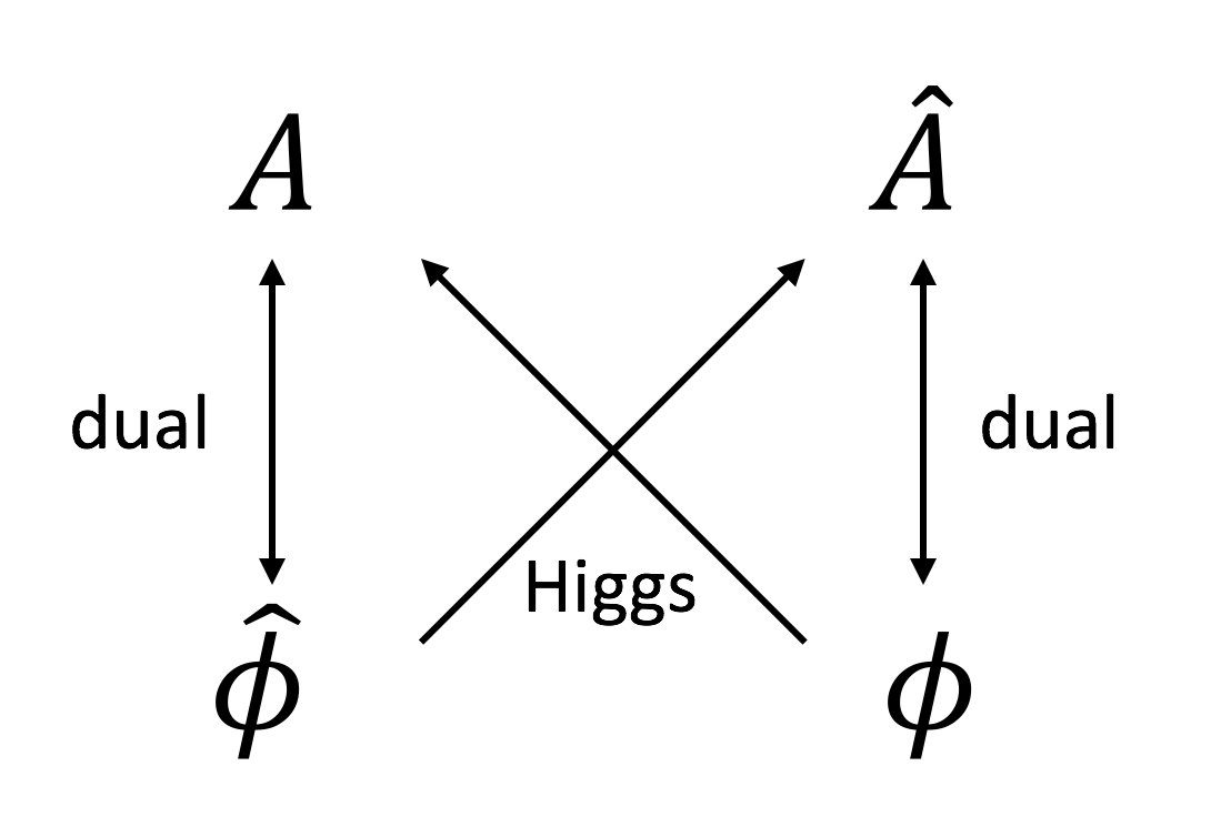
In this paper we study the versions of these two gauge theories. We construct them by adding matter fields with charge to the gauge theories and then Higgsing them to . In Section 2 we use the fact that the gauge symmetry of the -theory is the momentum symmetry of the -theory to add charge- fields that Higgs it to . Similarly, in Section 3 we add charge- fields to Higgs the -theory to . This is summarized in Figure 1.
Another convenient description of a continuum gauge theory is in terms of a -theory [30, 31, 32, 29]. We use this description in Section 4, which only involves the and the gauge fields but not the or fields. Certain aspects of this -type theory have been discussed in [8].
In Section 5, we show that the three different continuum theories in Sections 2, 3, and 4 are dual to each other. We will call these continuum field theories the tensor gauge theory.
The continuum tensor gauge theory describes the low-energy dynamics and the defects of the celebrated X-cube model [33] (see also [34]). In particular, it captures the restricted mobility of probe particles and the large ground state degeneracy of the X-cube model.
Crucial aspects of the analysis here rely on the understanding of the space of functions and the space of gauge fields in the four theories in [2]. This information determines which bundles are allowed, quantizes the coefficients in the Lagrangians, in the defects, and in the operators, and fixes the number of ground states.
As we said above, Appendix A reviews the representations of the cubic group and our notation and Appendix B reviews some aspects of the exotic global symmetries of [2].
Appendix C reviews the lattice description of gauge theories and their toric code presentation [35] and compares them with the continuum description of these theories. Even though this material is well known, we thought it would be helpful to present it here in order to clarify our perspective and to compare our various constructions to the known constructions of this well-studied case.
More specifically, our lattice gauge theories of and are similar to ordinary lattice gauge theories, while the X-cube model is analogous to the toric code. The ordinary gauge theory and the toric code are dual in the low energy, which is described by the continuum gauge theory. Analogously, our lattice theories of , and the X-cube model are dual to each other at long distances, which is captured by the continuum tensor gauge theory.
2 Tensor Gauge Theory
2.1 The Lattice Model
The first lattice tensor gauge theory is the version of the lattice gauge theory of in [1]. The X-cube model [33] on the dual lattice can be viewed as a limit of this lattice gauge theory with Gauss law dynamically imposed.
We start with a Euclidean lattice and label the sites by integers . Let be the number of sites along the direction. As in standard lattice gauge theory, the gauge transformations are phases on the sites. The gauge fields are phases placed on the (Euclidean) temporal links and on the spatial plaquettes , , . Note that there are no diagonal components of the gauge fields associated with the sites. The authors of [10] referred to a theory without these variables as a “hollow gauge theory.”
The gauge transformations act on them as
| (2.1) | ||||
and similarly for and . The Euclidean time-like links have standard gauge transformation rules (see (C.1)) and the plaquette elements are multiplied by the 4 phases around the plaquette.
The lattice action can include many gauge invariant terms. The simplest ones are associated with cubes in the time-space-space directions and in the space-space-space directions
| (2.2) | ||||
and similarly for the other directions.
In addition to the local gauge-invariant operators (LABEL:gaugeter), there are other non-local, extended ones. One example is a “strip” on the -plane:
| (2.3) |
and similarly for the other components in other directions. Here denotes the constant line on the -plane. More generally, the strip can be made out of plaquettes extending between and and zigzagging along a path on the -plane.
In the Hamiltonian formulation, we choose the temporal gauge to set all the ’s to 1. Let be the conjugate momenta of . They obey the Heisenberg algebra333By Heisenberg algebra, we mean the algebra generated by the clock and shift operators , satisfying and . This algebra arises in many different contexts and has many names. if they belong to the same plaquette, and commute otherwise.
Gauss law is imposed as an operator equation
| (2.4) |
where the product is an oriented product over the 12 plaquettes that share a common site .
The Hamiltonian is
| (2.5) |
The lattice model has a electric tensor symmetry whose conserved symmetry operator444When we discussed continuous symmetries, we used the phrase “charge” for the generator of infinitesimal transformations. Here, where the symmetry is discrete, we use “symmetry operator” for the generator of the symmetry. is proportional to
| (2.6) |
for each point on the -plane. There are similar symmetry operators along the other directions. This symmetry operator commutes with the Hamiltonian, in particular the terms. The electric tensor symmetry rotates the plaquette variables at for all by a phase. Using Gauss law (2.4), the dependence of the conserved operator on is a function of times a function of .
As in the standard gauge theory, instead of imposing the Gauss law as an operator equation, we can alternatively impose it energetically by adding a term to the Hamiltonian. One example of such Hamiltonian is
| (2.7) |
The limit gives the Hamiltonian of the X-cube model [33].
2.2 Continuum Lagrangian
We now present the continuum description for the lattice gauge theory of in Section 2.1. It is obtained by coupling the tensor gauge theory of to a charge- Higgs field . (See [2] for discussions on the - and -theories.) The Euclidean Lagrangian is:
| (2.8) |
The fields in the and in the are Lagrangian multipliers. The gauge transformation acts as
| (2.9) | ||||
with a -periodic gauge parameter.
The equations of motion are
| (2.10) | ||||
In particular, the equations of motion imply that the gauge-invariant field strengths of vanish:
| (2.11) | ||||
2.3 Global Symmetries
Let us track the global symmetries of the system from the and the tensor gauge theory of in [2].
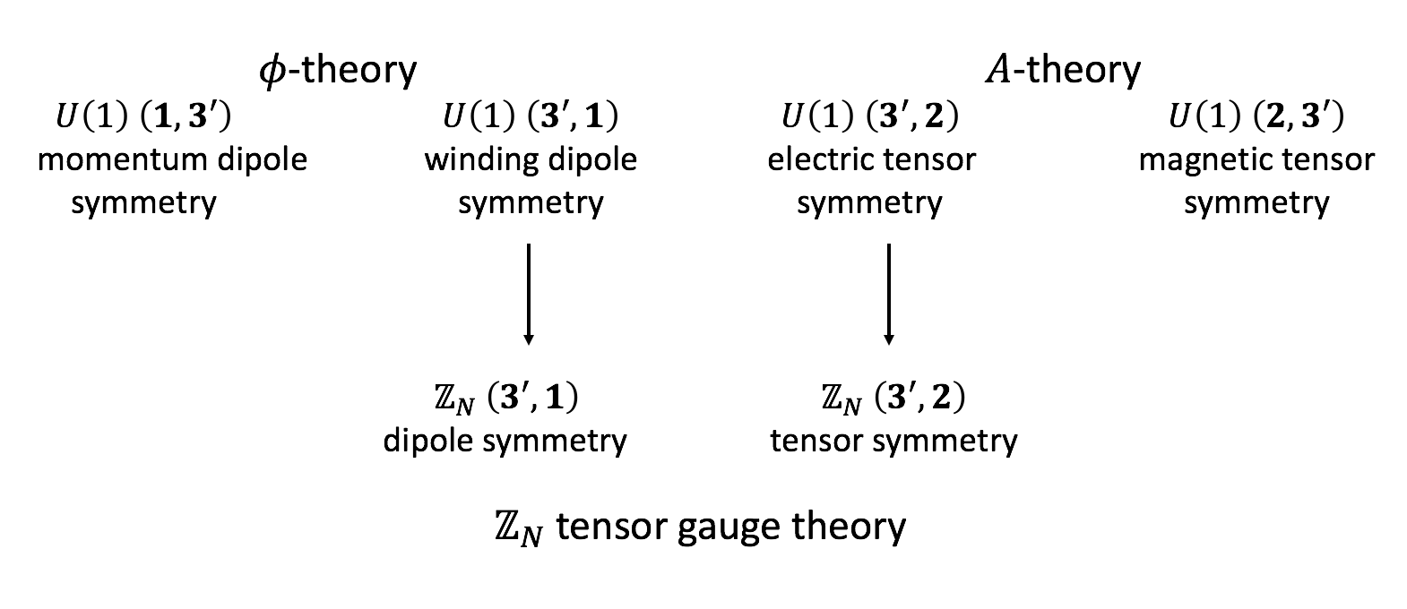
The scalar field theory of has a global momentum dipole symmetry and a global winding dipole symmetry. The momentum symmetry is gauged and the gauging turns the winding dipole symmetry into . In addition, the pure gauge theory of has a electric tensor symmetry and the coupling to the matter field breaks it to . Altogether, we have a dipole global symmetry and a tensor global symmetry. See Figure 3.
The tensor symmetry is the electric symmetry on the lattice (2.6). Its symmetry operator cannot be written in terms of the fields in the Lagrangian (2.8) in a local way.
The dipole symmetry is not present on the lattice (2.7). In the continuum, its symmetry operator is a strip in space
| (2.12) | ||||
where we have used the equation of motion (LABEL:eom1). Here is a closed curve on the -plane.
Only integer powers of the strip operator are invariant under the large gauge transformation
| (2.13) |
Furthermore, since the integral
| (2.14) |
is the quantized winding dipole charge of the -theory [2], we have . Therefore is a operator.
Similarly, there are strip operators along the other directions. They obey
| (2.15) | ||||
where is a closed curve on the -plane that wraps around the direction once but not the direction. See Appendix B.2 for a more abstract discussion of the dipole symmetry.
In Section 4.2, we will discuss these symmetry operators and their associated defects in more details.
2.4 Ground State Degeneracy
From the equation of motion (LABEL:eom1), we can solve all the other fields in terms of , and the solution space reduces to
| (2.16) |
In particular, there is no local excitation in the tensor gauge theory.
Let us enumerate the number of states in this system. Almost all configurations of can be gauged away completely, except for the winding modes (see [1, 2] for details on these winding modes in the -theory):
| (2.17) | ||||
where and . On a lattice, these winding modes are labeled by integers. Similarly, the gauge parameter can also have the above winding modes. Therefore, there are winding modes that cannot be gauged away with their valued in .
3 Tensor Gauge Theory
3.1 The Lattice Model
The X-cube model [33], with variables living on the links, can be viewed as a limit of another lattice gauge theory with Gauss law dynamically imposed. We now discuss this lattice gauge theory. Certain aspects of this lattice model have been discussed in [12].
We start with the Lagrangian formulation of this lattice model on a Euclidean lattice. The gauge parameters are phases placed on the sites. For each site , there are three gauge parameters in the satisfying at every site. (Recall that .) The gauge fields are phases placed on the links. Associated with each temporal link, there are three gauge fields in the satisfying . Associated with each spatial link along the direction, there is a gauge field in the .
The gauge transformations act on them as
| (3.1) | ||||
and similarly for and .
Let us discuss the gauge invariant local terms in the action. The first kind is a plaquette on the -plane:
| (3.2) |
and similarly for and . The second kind is a product of 12 spatial links around a cube in space at a fixed time:
| (3.3) | ||||
The Lagrangian for this lattice model is a sum over the above terms.
In addition to the local, gauge-invariant operators (3.3), there are other non-local, extended ones. For example, we have a line operator along the direction.
| (3.4) |
In the Hamiltonian formulation, we choose the temporal gauge to set all the ’s to 1. Let be the conjugate momenta for . They obey the Heisenberg algebra if they belong to the same link and commute otherwise. Gauss law is imposed as an operator equation
| (3.5) |
and similarly and . Note that identically, so the Gauss law operator is in the .


The Hamiltonian is
| (3.6) |
The lattice model has an electric dipole symmetry whose charge operators are
| (3.7) |
There are 4 other operators associated with the other directions. They commute with the Hamiltonian, in particular the terms. These two electric dipole symmetries rotate the phases of along a strip on the and planes, respectively.
Alternatively, we can impose Gauss law energetically by adding the following term to the Hamiltonian:
| (3.8) |
The limit gives the Hamiltonian of the X-cube model [33].
3.2 Continuum Lagrangian
We now present the continuum Lagrangian for the lattice gauge theory of in Section 3.1. The Euclidean Lagrangian is:555Recall that there are two presentations for a field in the of , and (see Appendix A). In the basis, the Lagrangian becomes (3.9)
| (3.10) |
where are gauge fields in the of and is a Higgs field in the with charge . and are Lagrangian multipliers in the and of , respectively.
The gauge symmetry is
| (3.11) | ||||
The equations of motion are
| (3.12) | ||||
In particular, the equations of motion imply that the gauge-invariant field strengths of vanish:
| (3.13) | ||||
In the above we have used .
Since there is no local operator in this theory, the low energy field theory is robust (see [1] for a discussion of robustness). Similarly, as above, since there are no local operators, the possible universality violation due to higher-derivative terms, which was discussed in [1, 2], is not present.
3.3 Global Symmetries
Let us track the global symmetries of the system from the and the tensor gauge theory of in [2].
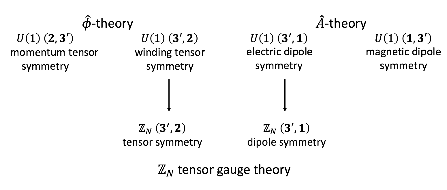
The field theory of has a global momentum tensor symmetry and a global winding tensor symmetry. The momentum symmetry is gauged and the gauging turns the winding tensor symmetry into . In addition, the pure gauge theory of has a electric dipole symmetry and the coupling to the matter field breaks it to . Altogether, we have a dipole global symmetry and a tensor global symmetry. See Figure 5. This is the same global symmetry in Section 2.3 for the tensor gauge theory of . Indeed, we will show that the two continuum tensor gauge theories of and are dual to each other in Section 5.1.
The dipole symmetry is the electric symmetry on the lattice (3.7). Its symmetry operator cannot be written in terms of the fields in the Lagrangian (3.10) in a local way.
The tensor symmetry is not present on the lattice (3.8). In the continuum, its symmetry operator is a line in space
| (3.14) |
where we have used the equation of motion (LABEL:eom2).
Only integer powers of are invariant under the large gauge transformation
| (3.15) |
Furthermore, since the integral
| (3.16) |
is the quantized winding tensor charge of the -theory [1], we have . Therefore is a operator.
Let us comment on the spatial dependence of . Since , we have
| (3.17) |
Hence the dependence of the symmetry operator on factorizes
| (3.18) |
Similarly, there are line operators along the other directions. See Appendix B.1 for a more abstract discussion of the tensor symmetry.
In Section 4.2, we will discuss these symmetry operators and their associated defects in more details.
3.4 Ground State Degeneracy
From (LABEL:eom2), we can solve all the other fields in terms of , and the solution space reduces to
| (3.19) |
Almost all configurations of can be gauged away, except for the winding modes (see [2] for details on these winding modes):
| (3.20) | ||||
where . There is an identification
| (3.21) | ||||
and similarly for the other ’s. If we regularize the space by a lattice, these winding modes are labeled by integers. Similarly, the gauge parameter can also have the above winding modes. Therefore, there are winding modes that cannot be gauged away with their valued in .
3.5 An Important Comment
When we studied the pure -theory (without gauge fields) in [2], we discussed configurations of the form
| (3.22) | ||||
The low-energy limit of the pure -theory has a global winding tensor symmetry. The winding charge of the configuration (3.22) is
| (3.23) |
Since it is not periodic in , is not a well-defined operator and therefore (3.22) violates the winding tensor symmetry. However, since these configurations lead to states with energy of order , while the states charged under that symmetry are at energy of order , it is meaningful to ignore such configurations in the continuum limit. As a result, the continuum -theory exhibits the accidental winding symmetry [2].
Let us turn now to the gauge theory. If instead of (3.10), we would have written the Lagrangian
| (3.24) |
then the situation would have been as in the pure -theory. The configurations (3.22) would have been suppressed by their large action.
The Lagrangian (3.10) is the low energy limit of (3.24). Then, the equation of motion (LABEL:eom2) relates (3.22) to
| (3.25) | ||||
The lack of periodicity in means that we need a transition function at ,666Viewed as real fields, the configuration (3.22) is not periodic in . However, since it is periodic in as a circle-valued function and since the gauge field (LABEL:strangehatA) is periodic in , there is no need for a transition function at .
| (3.26) |
This transition function is inconsistent because is not periodic in . Therefore, configurations like (3.22) are not allowed in the gauge theory.
The key point is the following. Considering only the space of fields, we can have configurations like (3.22) with trivial transition functions for the gauge field. (We do need transition functions for when we view them as real fields with transition functions, rather than as circle-valued fields.) Then, the equation of motion (LABEL:eom2), which is imposed as a constraint in the continuum field theory, ties to the gauge field and leads to the inconsistency.
We conclude that unlike the pure -theory in [2] or the gauge theory (3.24), where such configurations like (3.22) are allowed, but they are suppressed because of their action, here in (3.10) they are inconsistent with the gauge symmetry and must be excluded.
Even though configurations like (3.22) do not contribute, configurations of the form
| (3.27) | ||||
are consistent with the gauge symmetry. Furthermore, unlike the case in [2], they are not suppressed by their action and they must be included.
Let us explore some properties of (3.27). First, although of these configurations is ill-defined, of (3.27) is well-defined. This means that these configurations respect the subgroup of the winding tensor symmetry, which is the global symmetry of our gauge theory. In fact, for these configurations , i.e. they are not charged under this global symmetry. Second, these configurations can be gauged away by choosing a large gauge transformation parameter of the form (3.22). Therefore, they do not contribute new states in addition to the ground states we found above.
4 -type Tensor Gauge Theory
4.1 Continuum Lagrangian
We now discuss the third presentation of the tensor gauge theory [8].
This presentation involves the two gauge fields in Section 2 and 3:
| (4.1) | ||||
where we have written their representations on the right. They are subject to two gauge transformations. The first one is
| (4.2) | ||||
where is a periodic scalar. The second gauge transformation is
| (4.3) | ||||
where is periodic and transforms in the of . Their electric and magnetic fields are given in (LABEL:EB0) and (LABEL:hatEB0). See [2] for details on the and gauge fields.
The Euclidean Lagrangian is of the -type, i.e. it is a product of the gauge fields with the electric and magnetic fields for :
| (4.4) |
Integrating by parts, we can also write it as777We have used . Also note that .
| (4.5) |
The equations of motion set all the gauge-invariant local operators to zero:
| (4.6) |
While there are no local operators, there are gauge invariant extended operators, which generate exotic global symmetries. We will discuss this in detail in Section 4.2.
Since there are no local operators, the tensor gauge theory is robust (see [1] for a discussion of robustness). Small changes of the underlying microscopic model do not affect the long-distance field theory phase. In particular, the ground state degeneracy in Section 4.3 is also robust and cannot be lifted by small perturbations.
Similarly, as in the other two descriptions of the model, since there are no local operators, the possible universality violation due to higher-derivative terms, which was discussed in [1, 2], is not present. Therefore the results computed from this continuum Lagrangian are universal.
Quantization of the Level
Let us now discuss the quantization of the coefficient in (4.4) and (4.5). Similar to the ordinary -theories, the coefficient here will be quantized by large gauge transformation in the presence of nontrivial fluxes.
Consider the following large gauge transformation on a Euclidean 4-torus:
| (4.7) |
Under this gauge transformation, the action from (4.4) changes by
| (4.8) |
From [2], we have the following quantized fluxes
| (4.9) |
and similar fluxes for the other directions. Therefore for the path integral to be invariant under this large gauge transformation, we need
| (4.10) |
4.2 Defects and Operators
While there are no gauge-invariant local operators in the tensor gauge theory, there are gauge-invariant non-local, extended observables analogous to the Wilson lines in the (2+1)d Chern-Simons theory.
Fractons and Planons as Defects of
The simplest defect is a single particle of gauge charge at a fixed point in space . It is captured by the gauge-invariant defect
| (4.14) |
This immobile particle is identified as the probe limit of a fracton. The gauge charge is quantized by the large gauge transformation (4.7).
A pair of fractons of gauge charges separated, say, in the -direction, can move collectively. This is captured by the defect:
| (4.15) |
where is a spacetime curve in (but no ) representing the motion of a dipole of fractons on the -plane. It is a planon on the -plane.
Lineons and Planons as Defects of
The second kind of particle has three variants each associated with a spatial direction. A static particle of species and gauge charge is captured by the following defect
| (4.16) |
The gauge charge is quantized by a large gauge transformation . The particle of species, say, moving in the -direction is captured by the following line defect in spacetime
| (4.17) |
where is a spacetime curve on the -plane representing the motion of a particle along the -direction. The particle by itself cannot turn in space; it is confined to move along the -direction. This particle is the probe limit of the lineon.
While a single lineon of species is confined to move along the direction, a pair of them can move in more general directions. For example, a pair of lineons of species separated in the direction can move on the -plane. This motion is captured by the defect
| (4.18) |
where is a spacetime curve in representing a dipole of lineons, i.e. a planon, on the -plane.
Quasi-Topological Defects
If we deform infinitesimally the spacetime curve to a nearby one and similarly, the spacetime curve to a nearby one , the changes in these defects can be computed using the Stokes theorem:
| (4.19) | ||||
where is a surface bounded by and and is a surface bounded by and . In the tensor gauge theory, the equations of motion set , so these defects are invariant under small deformations of and in the appropriate manifold. Similar properties are true for defects along the other directions.
To conclude, these defects are topological under deformations along certain directions, but not all.
Symmetry Operators
In the special case when is a space-like curve on the -plane, reduces to the dipole symmetry operator (2.12). Similarly, in the special case when is a line along the direction at a fixed time, reduces to the tensor symmetry operator (3.14).
When the two symmetry operators and act at the same time with a curve in the -plane, they obey the commutation relation
| (4.20) |
Here is the intersection number between the curve and the line on the -plane.888At the risk of confusing the reader, we would like to point out that this lack of commutativity can be interpreted as a mixed anomaly between these two symmetries. See [29] for a related discussion on the relativistic one-form symmetries in the -dimensional gauge theory. There are similar commutation relations for operators in the other directions.
Next, consider a planon , say, separated in the direction with a spacetime curve in . In the special case when is a closed line along the direction at a fixed time and , reduces to a pair of tensor symmetry operators . The invariance (LABEL:quasitop) under small deformation of implies that is independent of . Indeed, this follows from (3.18) which we have discussed before.
4.3 Ground State Degeneracy
We now study the ground states of the tensor gauge theory on a spatial 3-torus using the presentation (4.4). The discussion will be similar to that in [8] and will extend it by paying attention to the global issues and the precise space of fields. The analysis proceeds similarly as the -dimensional tensor gauge theory in Section 7.5 of [1].
Let us choose the temporal gauge setting and . Then the phase space is
| (4.21) |
where we mod out the time-independent gauge transformations. The solution modulo gauge transformations is
| (4.22) | ||||
We have put in factors of for later convenience. The functions have mass dimension 1 while are dimensionless.
Only the sum of the zero modes for is physical, and similarly for . This implies a gauge symmetry for :
| (4.23) | ||||
There is a similar gauge symmetry for . As in [1], we define the gauge-invariant modes
| (4.24) |
They are subject to the constraint
| (4.25) |
Let us discuss the global periodicities of and . The large gauge transformation , with a piecewise continuous integer-valued function, implies that has a point-wise periodicity:
| (4.26) | ||||
and similarly for the direction and for the other components of .
On the other hand, the large gauge transformation
| (4.27) |
implies that has a point-wise delta function periodicity:
| (4.28) | ||||
for each , and
| (4.29) | ||||
for each . The other components of have similar periodicity.
The effective Lagrangian written in terms of and is
| (4.30) |
The Lagrangian for these modes is effectively -dimensional. In the strict continuum limit, the ground state degeneracy is infinite.
Let us regularize the degeneracy by placing the theory on a lattice. We will focus on the modes and , while the other modes can be done in parallel. On a lattice, we can solve in terms of and the other using (4.25). The remaining, unconstrained ’s have periodicities for each . On the other hand, we can use the gauge symmetry (LABEL:fhatgauge) to gauge fix . The remaining ’s have periodicities for each . The effective Lagrangian is now written in terms of pairs of variables .
Each pair leads to an -dimensional Hilbert space. Combining the modes from the other directions, we end up with the expected ground state degeneracy .
Ground State Degeneracy from Global Symmetries
The ground state degeneracy can be understood from the global symmetries. Let us focus on a subset of the symmetry operators: the tensor symmetry operator extended along the direction (3.14)
| (4.31) |
and the dipole symmetry strip operators on the -plane (2.12)
| (4.32) |
Here is a curve on the -plane that wraps around direction once but not the direction and similarly with . Due to the topological property (LABEL:quasitop), these strip operators on the -plane do not depend on their coordinates. These operators obey commutation relations similar to (4.20):
| (4.33) | ||||
and they commute otherwise.
On a lattice, due to (3.18), we have tensor symmetry operators (4.31) along the direction. Similarly, due to (LABEL:Wrelation), we have dipole symmetry operators (4.32) on the plane. The commutation relations between these operators are isomorphic to copies of the Heisenberg algebra, and . The isomorphism is given by
| (4.34) | ||||
where is a strip operator along the direction with width , and similarly for .
Combining the symmetry operators from the other directions, the commutation relations force the ground state degeneracy to be .999For ordinary -dimensional gauge theory on a 2-torus, the electric and magnetic one-form global symmetries give rise to 2 pairs of Heisenberg algebra. Hence the ground state degeneracy is .
5 Dualities
In this section we discuss the dualities of our continuum and lattice theories.
In Section 5.1, we show that the continuum theory of (Section 2.2), that of (Section 3.2), and the -type theory (Section 4.1) are dual to each other. These are exact dualities of continuum field theories.
In Section 5.2, we show that the lattice theory of (Section 2.1), that of (Section 3.1), and the X-cube model are dual to each other at long distances. These are infrared dualities. The low energy limit is the continuum tensor gauge theory. We further discuss the global symmetries of these lattice models.
5.1 The Three Continuum Descriptions
We now show the equivalence between the three different presentations, (2.8), (3.10), and (4.4), of the tensor gauge theory by duality transformations.
We first show that (2.8) and (4.4) are dual to each other. We start with (2.8)
| (5.1) |
where are the tensor gauge fields and is a -periodic real scalar field that Higgses the gauge symmetry to . The fields in the and in the are the Lagrangian multipliers.
We rewrite the Lagrangian as
| (5.2) |
Now we interpret the Higgs field as a Lagrangian multiplier implementing the constraint
| (5.3) |
Locally, the constraint is solved by gauge fields in the :
| (5.4) | ||||
(5.2) then reduces to (4.4). Hence we have shown the equivalence between (2.8) and (4.4).
Next we show that (3.10) is dual to (4.4). We start with (3.10):
| (5.5) |
where are gauge fields in the of and is a Higgs field in the with charge . and are Lagrangian multipliers in the and of , respectively. We can rewrite the Lagrangian as
| (5.6) |
where we have used . We now interpret the Higgs field as a Lagrangian multiplier implementing the constraint
| (5.7) |
This constraint can be locally solved by gauge fields in the :
| (5.8) | ||||
(5.6) then reduces to (4.5). Finally, we integrate (4.5) by parts to arrive at (4.4).
5.2 X-Cube Model and the Lattice Tensor Gauge Theories
In this subsection we realize the X-cube model as limits of the lattice gauge theories of (Section 2.1) and (Section 3.1). We further discuss the global symmetries of these three lattice theories.
Lattice Gauge Theory of
As discussed in Section 2.1, the lattice theory has an electric tensor global symmetry. Its conserved symmetry operator is a line in the, say, direction and at a fixed point (2.6):
| (5.9) |
Gauss law (2.4), which is strictly imposed, implies that the dependence of factorizes:
| (5.10) |
Similarly, there are conserved operators along the other directions. These are recognized as the symmetry operators tensor global symmetry in Appendix B.1.
Note that the dipole global symmetry in the continuum (2.2) is not present on the lattice.
Lattice Gauge Theory of
As discussed in Section 3.1, the lattice theory has an electric dipole global symmetry. Its conserved symmetry operator is proportional to
| (5.11) |
where the product is over a zigzagging closed curve on the plane (see Figure 6). Special cases of such strip operators are in (3.7).
Gauss law (LABEL:hatlatticegauss), which is strictly imposed, implies that is invariant under small changes of . In other words, the dependence of on is topological. Similarly, there are conserved operators along the other directions. These are recognized as the symmetry operators for the tensor global symmetry in Appendix B.2.101010In the continuum limit, is identified with in Appendix B.2 where is the lattice spacing.
Note that the tensor global symmetry in the continuum (3.2) is not present on the lattice.
X-Cube Model
The X-cube model [33] can be realized as the limit of the lattice gauge theory of (3.8)
| (5.12) |
where the individual terms are defined in Section 3.1 and Figure 4. Note that there are no gauge symmetry or Gauss law in the X-cube model.
The X-cube model has two kinds of global symmetries. The conserved symmetry operator of the first kind is the Wilson line operator (3.4)
| (5.13) |
Similarly there are other line operators along the other directions. These are the string-like logical operators of the X-cube model.
Unlike the symmetry operator (5.9) in the lattice gauge theory of , the dependence of (5.13) does not factorize as in (5.10). It is the unconstrained tensor global symmetry in Appendix B.1.
The conserved symmetry operator of the second kind is (5.11). However, in the X-cube model, the operator depends not only on the topology of the curve , but also the detailed shape of it. Similarly there are other line operators along the other directions. These are the membrane-like logical operators of the X-cube model. It is the unconstrained dipole global symmetry in Appendix B.2.
Dually, the X-cube model can also be realized as the limit of the lattice gauge theory of (2.7) on the dual lattice. In this presentation, the unconstrained tensor symmetry is the electric symmetry (2.6). On the other hand, the symmetry operator of the unconstrained dipole symmetry is the Wilson strip (2.3).
These unconstrained tensor and dipole symmetries are analogous to the non-relativistic electric and magnetic one-form symmetries of the toric code [6]. At long distances, they become the tensor and dipole symmetries of the continuum tensor gauge theory (see Section 2.3, 3.3, and 4.2).
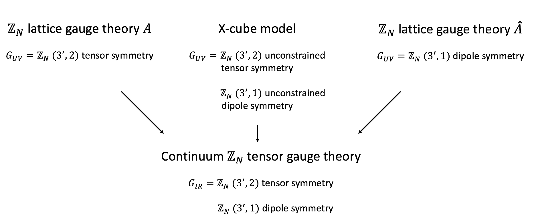
We conclude that the lattice gauge theory of , that of , and the X-cube model are dual to each other at long distances. We summarize their global symmetries on the lattice and in the continuum in Figure 7.
Acknowledgements
We thank X. Chen, M. Cheng, M. Fisher, A. Gromov, M. Hermele, P.-S. Hsin, A. Kitaev, D. Radicevic, L. Radzihovsky, S. Sachdev, D. Simmons-Duffin, S. Shenker, K. Slagle, D. Stanford for helpful discussions. We also thank P. Gorantla, H.T. Lam, D. Radicevic, and T. Rudelius for comments on the manuscript. The work of N.S. was supported in part by DOE grant DESC0009988. NS and SHS were also supported by the Simons Collaboration on Ultra-Quantum Matter, which is a grant from the Simons Foundation (651440, NS). Opinions and conclusions expressed here are those of the authors and do not necessarily reflect the views of funding agencies.
Appendix A Cubic Group and Our Notations
The symmetry group of the cubic lattice (up to translations) is the cubic group, which consists of 48 elements. We will focus on the group of orientation-preserving symmetries of the cube, which is isomorphic to the permutation group of four objects .
The irreducible representations of are the trivial representation , the sign representation , a two-dimensional irreducible representation , the standard representation , and another three-dimensional irreducible representation . is the tensor product of the sign representation and the standard representation, .
It is convenient to embed and decompose the known irreducible representations in terms of representations. The first few are
| (A.1) | ||||||
We will label the components of representations using vector indices as follows. The three-dimensional standard representation of carries an vector index , or equivalently, an antisymmetric pair of indices .111111We will adopt the convention that indices in the square brackets are antisymmetrized, whereas indices in the parentheses are symmetrized. For example, and . Similarly, the irreducible representations of can be expressed in terms of the following tensors:
| (A.2) | ||||||||
In the above we have two different expressions, and , for the irreducible representation of . In the first expression, is the component of in the tensor product . In the second expression, is the component of in the tensor product . The two bases of tensors are related as121212There is a third expression for the : with . Repeated indices are not summed over here. This expression is most natural if we embed the of into the of (i.e. symmetric, traceless rank-two tensor). It is related to the first expression as .
| (A.3) | ||||
Appendix B Exotic Global Symmetries
In this appendix we review the tensor and dipole global symmetries of [2]. We will first discuss the versions of these symmetries and their currents, and then generalize to . The space is assumed to be a 3-torus with lengths .
B.1 Tensor Global Symmetry
The versions of the following two tensor global symmetries are realized in the and the theories in [2].
Tensor Symmetry
Consider the tensor symmetry with currents in the representations. The current conservation equation is
| (B.1) |
The symmetry operator is the exponentiation of the conserved charge :
| (B.2) | ||||
which is a “slab” of width in the direction and extends along the directions. Since ,
| (B.3) |
On a lattice, we have such symmetry operators.
If the symmetry group is as opposed to , then there are no currents but only the symmetry operators with and .
Tensor Symmetry
Next, consider a different tensor global symmetry with currents in the representations. The currents obey the conservation equation
| (B.4) |
and the differential constraint
| (B.5) |
The symmetry operator is a line extended in the direction at a fixed point on the -plane:
| (B.6) |
The differential condition (LABEL:gauss1) implies that the position dependence of factorizes
| (B.7) |
and only the product of their zero modes is physical. On a lattice, we have such symmetry operators.
If the symmetry group is as opposed to , then there are no currents but only the symmetry operators with and .
Unconstrained Tensor Symmetry
We can also consider a variant of the tensor symmetry where the differential constraint (LABEL:gauss1) is relaxed. Consequently, the symmetry operator does not obey (B.7). We will call this variant the unconstrained tensor symmetry. Such a unconstrained tensor symmetry is present in the X-cube model (see Section 5.2). The relation between the unconstrained tensor and the tensor symmetries is analogous to that between the non-relativistic [6] and the relativistic one-form symmetries [29].
B.2 Dipole Global Symmetry
The versions of the following two dipole global symmetries are realized in the and the theories in [2].
Dipole Symmetry
Consider the dipole symmetry generated by currents in the of . They obey
| (B.8) | ||||
The symmetry operator is a slab with finite width in the direction and extend in the direction
| (B.9) |
They obey
| (B.10) |
On a lattice, we have such symmetry operators.
If the symmetry group is as opposed to , then there are no currents but only the symmetry operators with and .
Dipole Symmetry
The second dipole symmetry is generated by currents with of . They obey the conservation equation:
| (B.11) |
and a differential condition
| (B.12) |
The symmetry operator is a strip operator:
| (B.13) |
Here the strip is the direct product of the segment and a closed curve on the -plane. The differential condition (B.12) implies that the symmetry operator is independent of small deformation of the curve . In other words, the dependence on is topological.
Similarly, we have symmetry operators along the other directions. They obey
| (B.14) | ||||
where is any closed curve on the -plane that wraps around the direction once but not the direction. On a lattice, we have such symmetry operators.
If the symmetry group is as opposed to , then there are no currents but only the symmetry operators with and .
Unconstrained Dipole Symmetry
We can also consider a variant of the dipole symmetry where the differential constraint (B.12) is relaxed. Consequently, the symmetry operator depends on the detailed shape of the curve . We will call this variant the unconstrained dipole symmetry. Such a unconstrained dipole symmetry is present in the X-cube model (see Section 5.2). Again, the relation between the unconstrained dipole and the dipole symmetries is analogous to that between the non-relativistic [6] and the relativistic one-form symmetries [29].
Appendix C Gauge Theory and Toric Code
This appendix reviews various presentations of ordinary gauge theories. The purpose of this review is to demonstrate, in a well-known setting, the various approaches that we use in the body of the paper when we study more sophisticated gauge theories.
C.1 The Lattice Model
Lattice Gauge Theory
We start with a Euclidean -dimensional cubic lattice, whose sites are labeled by integers . The degrees of freedom are group elements on the links. The gauge transformation parameters are elements on the sites and they act on as
| (C.1) |
and similarly for , etc. The simplest gauge invariant interaction involves an oriented product of around a plaquettes
| (C.2) |
More complicated interactions are also possible.
The lattice gauge theory includes magnetic excitations, but it has no electric excitations. Correspondingly, it does not have a magnetic global symmetry, but it does have an electric one-form global symmetry [29]. The one-form symmetry multiplies all the link variables by arbitrary phases such that their oriented product around every plaquette, as in (C.2), is one. Most of these transformations are gauge transformations, but those that are not gauge transformations act as a global symmetry. The objects charged under this one-form global symmetry are Wilson lines – products of s along closed curves.
In the Hamiltonian formulation, we use the analog of temporal gauge setting all the links in the time direction to one, i.e. . We also introduce “momenta” conjugate to on the links. ( was a Euclidean spacetime direction and is a spatial direction.) They are conjugate variables in the sense that and on the same link satisfy a Heisenberg algebra
| (C.3) |
and elements on different links commute. In addition, we need to impose Gauss law. It is an operator constraint at every site given by
| (C.4) |
where the product of s includes all the link variables connected to the site .
Toric Code
It is common, following [35, 36], not to impose Gauss law (C.4) as an operator constraint, but instead, to add a term to the Hamiltonian to raise the energy of states violating it. The simplest such Hamiltonian is the toric code:
| (C.5) |
The first term imposes the Gauss law energetically. The low-lying states satisfy , but excited states do not satisfy it. Once such a term is added to the Hamiltonian there is no need to preserve the underlying gauge symmetry and more interactions can be added, e.g. .
The toric code includes both electrically-charged and magnetically-charged dynamical excitations. Therefore, it does not have global electric or magnetic generalized symmetries of the kind studied in [29]. Instead, it has the non-relativistic electric and magnetic one-form global symmetries studied in [6]. If additional terms, e.g. , are added to the Hamiltonian, even the non-relativistic electric symmetry is violated [6]. Similarly, additional terms like break the non-relativistic magnetic symmetry.
These two lattice systems, the ordinary lattice gauge theory and the toric code, have the same low-energy limit. In other words, they are dual to each other in the infrared. We will now discuss this continuum gauge theory.
C.2 Continuum Lagrangians
The Three Dual Descriptions of the Continuum Theory
There are several presentations of the continuum gauge theory. One presentation is in terms of an ordinary gauge theory with a gauge field (which is locally a one-form) coupled to a charge- scalar Higgs field . The gauge group is then Higgsed from to . The Lagrangian is131313Since unlike in the body of the paper this system is relativistic, we use form notation.
| (C.6) |
Here is an independent -form field. It acts as a Lagrange multiplier setting . This Higgses to . This presentation of the gauge theory is similar to the one used in Section 2.
Instead of using (C.6), we can follow [30, 31, 32, 29] and dualize the scalar to a -form gauge field. The resulting Lagrangian is
| (C.7) |
where is a -form gauge field.141414Often, this Lagrangian is written as and hence the name -theory. Since we use the letter for a magnetic field, we write it in terms of . It is related to in (C.6) through . This presentation of the theory is similar to the one in Section 4.
We can also further dualize to a -form gauge field to convert (C.7) to
| (C.8) |
Here is a two-form field. It is a Lagrangian multiplier enforcing . In this presentation, the gauge symmetry of is Higgsed to .
This presentation of the theory is similar to the one in Section 3.
It should be noted that the presentation (C.8) motivates another lattice construction of the same system. Here the continuum gauge field is replaced by a gauge field on -dimensional cubes, whose gauge parameters take values on -dimensional cubes. This is similar to the discussion in Section 3.1.
Defects and Operators
The continuum gauge theory has neither electric nor magnetic excitations. Such excitations, if present, have high energy of the order to the lattice scale. Therefore, they are effectively classical. This means that the low-energy effective theory has both an electric and a magnetic generalized global symmetry [29].
The physics of massive probes charged under the above generalized global symmetries is captured by operators/defects. This is most clear in the presentation (C.7), where the natural observables are
| (C.9) |
Here, the integrals are over a 1-dimensional curve and a -dimensional manifold in spacetime, respectively. These represent electric and the magnetic objects .
If such operators act at the same time and they pierce each other, they do not commute. Therefore, is the operator generating the magnetic symmetry and is the operator generating the electric symmetry. See [29] for more details. Also, since these operators act in the space of ground states, we can interpret these global symmetries as being spontaneously broken.151515In quantum information theory such operators are referred to as logical operators. We thank M. Hermele for a helpful discussion about it. We emphasize that even when the lattice system does not have these global symmetries, these symmetries arise as accidental symmetries acting in the low-energy theory.
Finally, when the low-energy theory does not have any local, gauge-invariant operators. Therefore, it is robust. (See [1].) Its accidental higher-form global symmetries cannot be ruined and the structure of the ground states cannot be changed by any short-distance perturbation, provided it is small enough. This is similar to the -dimensional continuum tensor gauge theory of this paper.
References
- [1] N. Seiberg and S.-H. Shao, Exotic Symmetries, Duality, and Fractons in 2+1-Dimensional Quantum Field Theory, arXiv:2003.10466.
- [2] N. Seiberg and S.-H. Shao, Exotic Symmetries, Duality, and Fractons in 3+1-Dimensional Quantum Field Theory, arXiv:2004.00015.
- [3] P. Gorantla, H. T. Lam, N. Seiberg, and S.-H. Shao, More Exotic Field Theories in 3+1 Dimensions, arXiv:2007.04904.
- [4] R. M. Nandkishore and M. Hermele, Fractons, Ann. Rev. Condensed Matter Phys. 10 (2019) 295–313, [arXiv:1803.11196].
- [5] M. Pretko, X. Chen, and Y. You, Fracton Phases of Matter, arXiv:2001.01722.
- [6] N. Seiberg, Field Theories With a Vector Global Symmetry, SciPost Phys. 8 (2020) 050, [arXiv:1909.10544].
- [7] C. Xu and C. Wu, Resonating plaquette phases in su(4) heisenberg antiferromagnet, Physical Review B 77 (Apr, 2008).
- [8] K. Slagle and Y. B. Kim, Quantum Field Theory of X-Cube Fracton Topological Order and Robust Degeneracy from Geometry, Phys. Rev. B96 (2017), no. 19 195139, [arXiv:1708.04619].
- [9] D. Bulmash and M. Barkeshli, The Higgs Mechanism in Higher-Rank Symmetric Gauge Theories, Phys. Rev. B97 (2018), no. 23 235112, [arXiv:1802.10099].
- [10] H. Ma, M. Hermele, and X. Chen, Fracton topological order from the Higgs and partial-confinement mechanisms of rank-two gauge theory, Phys. Rev. B98 (2018), no. 3 035111, [arXiv:1802.10108].
- [11] Y. You, T. Devakul, F. J. Burnell, and S. L. Sondhi, Symmetric Fracton Matter: Twisted and Enriched, arXiv:1805.09800.
- [12] D. Radicevic, Systematic Constructions of Fracton Theories, arXiv:1910.06336.
- [13] A. Rasmussen, Y.-Z. You, and C. Xu, Stable Gapless Bose Liquid Phases without any Symmetry, arXiv e-prints (Jan., 2016) arXiv:1601.08235, [arXiv:1601.08235].
- [14] M. Pretko, Subdimensional Particle Structure of Higher Rank U(1) Spin Liquids, Phys. Rev. B95 (2017), no. 11 115139, [arXiv:1604.05329].
- [15] M. Pretko, Generalized Electromagnetism of Subdimensional Particles: A Spin Liquid Story, Phys. Rev. B96 (2017), no. 3 035119, [arXiv:1606.08857].
- [16] M. Pretko, Higher-Spin Witten Effect and Two-Dimensional Fracton Phases, Phys. Rev. B96 (2017), no. 12 125151, [arXiv:1707.03838].
- [17] A. Gromov, Chiral Topological Elasticity and Fracton Order, Phys. Rev. Lett. 122 (2019), no. 7 076403, [arXiv:1712.06600].
- [18] M. Pretko and L. Radzihovsky, Fracton-Elasticity Duality, Phys. Rev. Lett. 120 (2018), no. 19 195301, [arXiv:1711.11044].
- [19] K. Slagle, A. Prem, and M. Pretko, Symmetric Tensor Gauge Theories on Curved Spaces, Annals Phys. 410 (2019) 167910, [arXiv:1807.00827].
- [20] M. Pretko, The Fracton Gauge Principle, Phys. Rev. B98 (2018), no. 11 115134, [arXiv:1807.11479].
- [21] D. J. Williamson, Z. Bi, and M. Cheng, Fractonic Matter in Symmetry-Enriched U(1) Gauge Theory, Phys. Rev. B100 (2019), no. 12 125150, [arXiv:1809.10275].
- [22] A. Gromov, Towards classification of Fracton phases: the multipole algebra, Phys. Rev. X9 (2019), no. 3 031035, [arXiv:1812.05104].
- [23] M. Pretko, Z. Zhai, and L. Radzihovsky, Crystal-to-Fracton Tensor Gauge Theory Dualities, Phys. Rev. B100 (2019), no. 13 134113, [arXiv:1907.12577].
- [24] Y. You, Z. Bi, and M. Pretko, Emergent fractons and algebraic quantum liquid from plaquette melting transitions, Phys. Rev. Res. 2 (2020), no. 1 013162, [arXiv:1908.08540].
- [25] Y. You, F. J. Burnell, and T. L. Hughes, Multipolar Topological Field Theories: Bridging Higher Order Topological Insulators and Fractons, arXiv:1909.05868.
- [26] V. B. Shenoy and R. Moessner, -fractonic Maxwell theory, Phys. Rev. B 101 (2020), no. 8 085106, [arXiv:1910.02820].
- [27] A. Gromov, A. Lucas, and R. M. Nandkishore, Fracton hydrodynamics, arXiv:2003.09429.
- [28] O. Dubinkin, A. Rasmussen, and T. L. Hughes, Higher-form Gauge Symmetries in Multipole Topological Phases, arXiv:2007.05539.
- [29] D. Gaiotto, A. Kapustin, N. Seiberg, and B. Willett, Generalized Global Symmetries, JHEP 02 (2015) 172, [arXiv:1412.5148].
- [30] J. M. Maldacena, G. W. Moore, and N. Seiberg, D-brane charges in five-brane backgrounds, JHEP 10 (2001) 005, [hep-th/0108152].
- [31] T. Banks and N. Seiberg, Symmetries and Strings in Field Theory and Gravity, Phys. Rev. D83 (2011) 084019, [arXiv:1011.5120].
- [32] A. Kapustin and N. Seiberg, Coupling a QFT to a TQFT and Duality, JHEP 04 (2014) 001, [arXiv:1401.0740].
- [33] S. Vijay, J. Haah, and L. Fu, Fracton Topological Order, Generalized Lattice Gauge Theory and Duality, Phys. Rev. B94 (2016), no. 23 235157, [arXiv:1603.04442].
- [34] C. Castelnovo, C. Chamon, and D. Sherrington, Quantum mechanical and information theoretic view on classical glass transitions, Phys. Rev. B 81 (May, 2010) 184303.
- [35] A. Yu. Kitaev, Fault tolerant quantum computation by anyons, Annals Phys. 303 (2003) 2–30, [quant-ph/9707021].
- [36] L. Balents, M. P. A. Fisher, and S. M. Girvin, Fractionalization in an easy-axis Kagome antiferromagnet, Phys. Rev. B65 (2002) 224412, [cond-mat/0110005].