Witnessing latent time correlations with a single quantum particle

Abstract

When a noisy communication channel is used multiple times, the errors occurring at different times generally exhibit correlations. Classically, these correlations do not affect the evolution of individual particles: a single classical particle can only traverse the channel at a definite moment of time, and its evolution is insensitive to the correlations between subsequent uses of the channel. In stark contrast, here we show that a single quantum particle can sense the correlations between multiple uses of a channel at different moments of time. Taking advantage of this phenomenon, it is possible to enhance the amount of information that the particle can reliably carry through the channel. In an extreme example, we show that a channel that outputs white noise whenever the particle is sent at a definite time can exhibit correlations that enable a perfect transmission of classical bits when the particle is sent at a superposition of two distinct times. In contrast, we show that, in the lack of correlations, a single particle sent at a superposition of two times undergoes an effective channel with classical capacity of at most 0.16 bits. When multiple transmission lines are available, time correlations can be used to simulate the application of quantum channels in a coherent superposition of alternative causal orders, and even to provide communication advantages that are not accessible through the superposition of causal orders.

I Introduction

Quantum communication enables new possibilities that were unthinkable in the classical world, notably including secure key distribution Bennett and Brassard (1984); Ekert (1991). The main hurdle to the implementation of quantum communication, however, is the fragility of quantum states to noise. To tackle this problem, quantum error correction schemes encode information into multiple quantum particles, using redundancy to mitigate the effects of noise Shor (1995); Gottesman (2010); Lidar and Brun (2013).

When the same communication channel is used multiple times, the noisy processes experienced by particles sent at different times are generally correlated Macchiavello and Palma (2002); Kretschmann and Werner (2005); Caruso et al. (2014); Pollock et al. (2018). For example, photons transmitted through an optical fibre are subject to random changes in their polarisation Ball and Banaszek (2005), and since such changes happen on a finite timescale, photons sent at nearby times experience approximately the same noisy processes. A similar situation arises in satellite quantum communication, where the satellite’s motion induces dynamical mismatches of reference frame with respect to the ground station Bonato et al. (2006).

The presence of correlations is both a threat and an opportunity for communication. On the one hand, it can undermine the effectiveness of standard error correcting schemes, which assume independent errors on the transmitted particles. On the other hand, tailored codes that exploit the correlations among different particles can enhance the transmission of information Macchiavello and Palma (2002); Chiribella et al. (2011); Giovannetti and Fazio (2005); Macchiavello et al. (2004); Ruggeri et al. (2005); Cerf et al. (2005); Giovannetti and Mancini (2005); Ball et al. (2004); Banaszek et al. (2004); Caruso et al. (2014); Bowen and Mancini (2004); Plenio and Virmani (2007); Bayat et al. (2008); Karpov et al. (2006); Memarzadeh et al. (2011); Xiao et al. (2016); D’Arrigo et al. (2012).

Like most error correcting schemes, the existing codes for correlated noise use multiple physical particles to encode a single logical message. Classically, the use of multiple particles is essential: since a single classical particle can only traverse a communication channel at a definite moment of time, correlations between different uses of the channel do not affect the particle’s evolution. The same conclusion holds even if the moment of transmission is chosen at random: in this case, the resulting evolution is simply the average of the evolutions associated to each individual moment of time, and the overall evolution is independent of the time correlations.

In stark contrast, here we show that a single quantum particle can sense the correlations between multiple uses of the same quantum communication channel. At the fundamental level, this effect is made possible by the ability of quantum particles to experience a coherent superposition of multiple time-evolutions Aharonov et al. (1990); Oi (2003); Åberg (2004a); Gisin et al. (2005); Abbott et al. (2020); Chiribella and Kristjánsson (2019); Dong et al. (2019); Vanrietvelde and Chiribella (2021). In particular, we will consider the situation in which the particle is in a superposition of travelling at different moments of time, as illustrated in Figure 1. Taking advantage of the time correlations in the noise, we show that it is possible to enhance the amount of information that a single particle can carry from a sender to a receiver, beating the ultimate limit achievable in the lack of correlations.

We demonstrate this effect with an extreme example, in which a single quantum particle carries one bit of classical information through a transmission line that completely erases information at every definite time step. This phenomenon witnesses the presence of correlations between different uses of the transmission line: in the lack of correlations, we show that the number of bits that can be reliably transmitted by sending a single particle at a superposition of two different times does not exceed 0.16.

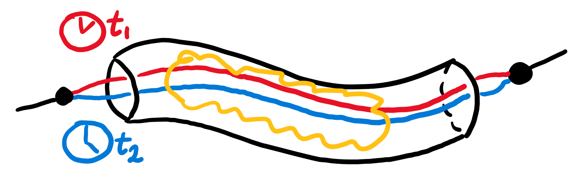
Figure 1: A single quantum particle can travel through a transmission line at a superposition of two different moment of time $t_{1}$ (red) and $t_{2}$ (blue). Along the way, the particle experiences errors (yellow region), and the errors occurring at time $t_{1}$ are generally correlated with the errors occurring at time $t_{2}$. By taking advantage of these correlations, the errors can be mitigated or even completely removed.

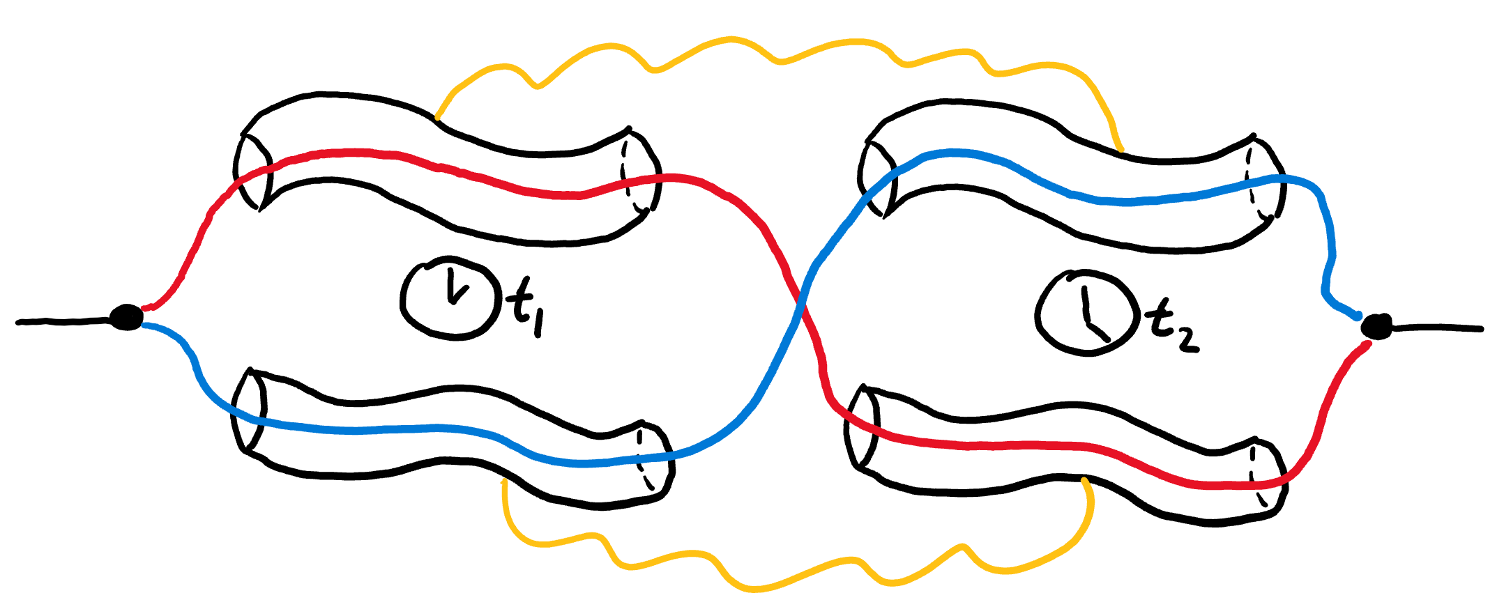
Figure 2: A single particle can travel on a superposition of two different paths (red and blue), which traverse two transmission lines (top and bottom) at two moments of time $t_{1}$ and $t_{2}$. The errors occurring on successive uses of the same transmission line are correlated (yellow lines), so the particle experiences correlated errors across the two branches (red and blue) of the superposition. These time correlations are a resource that can be used to mimic the use of quantum channels in a superposition of orders, and even to achieve larger communication advantages.

It is worth stressing that the above advantage is not specific to time correlations, but applies more generally to spatial correlations, or to other types of correlations: as long as two different uses of a channel are correlated, one may take advantage of the correlations by sending a quantum particle in a superposition of going through one use or the other.

Time-correlated channels are also interesting for foundational reasons. Recently, they have been proposed as a way to reproduce the use of quantum channels in a superposition of different causal orders Oreshkov (2019); Chiribella and Kristjánsson (2019). In particular, they have been used to reproduce the action of the quantum SWITCH Chiribella et al. (2009a, 2013), a higher-order operation that combines two variable quantum channels in a superposition of two alternative orders. In practice, time-correlated channels underlie all the existing experimental setups inspired by the quantum SWITCH Procopio et al. (2015); Rubino et al. (2017); Goswami et al. (2018); Guo et al. (2020); Goswami et al. (2020); Goswami and Romero (2020); Rubino et al. (2021).

The quantum SWITCH is known to offer a number of advantages in quantum communication Ebler et al. (2018); Salek et al. (2018); Chiribella et al. (2021); Goswami et al. (2020); Procopio et al. (2019, 2020); Chiribella et al. (2020). Here we show that (1) time correlations are essential in order to reproduce the advantages of the quantum SWITCH, and (2) the access to time-correlated channels is an even more powerful resource than the ability to combine ordinary quantum channels in a superposition of alternative orders.

To make the above points, we consider the scenario illustrated in Figure 2, where a single particle is sent on a superposition of two paths, traversing two independent channels, each with the property that different uses of the same channel at different moments of time are correlated, while the action of the channel at any given time is completely depolarising. When the noise is perfectly correlated, the network in Figure 2 reproduces the quantum SWITCH of two completely depolarising channels, which is known to achieve a communication capacity of 0.049 Ebler et al. (2018); Chiribella et al. (2020). In contrast, we show that in the lack of time correlations the maximum capacity achieved by sending a particle on a superposition of paths is at most 0.024 bits. This result proves that, in this scenario, the physical origin of the communication advantage of the quantum SWITCH is not merely the superposition of paths, but rather the interplay between the superposition of paths and the time correlations in the noise.

Remarkably, we also find that the time correlations that reproduce the action of the quantum SWITCH are not the most favourable for the transmission of classical information: while the quantum SWITCH of two completely depolarising channels can at most yield 0.049 bits of classical communication Ebler et al. (2018); Chiribella et al. (2020), a more sophisticated pattern of time correlations yields the communication of at least 0.31 bits. The gap between these two values further highlights the power of time correlations, which are not only capable of reproducing the benefits of the superposition of causal orders, but also of surpassing them.

The remainder of the paper is structured as follows. In Section II we describe the formalism of time-correlated channels and derive the effective evolution experienced by a single particle upon entering a time-correlated channel at a superposition of times. In Section III, we consider the transmission of a single particle at a superposition of times, as in Figure 1, and we demonstrate that the correlations between different uses of the channels offer a communication advantage over all communication scenarios where the channels are uncorrelated. In Section IV, we consider the network scenario of Figure 2, and we show that time correlations are necessary to reproduce the advantages of the quantum SWITCH, and that certain time correlations can even offer higher advantages. Finally, we discuss the effects of noise on the control degree of freedom in Section V and conclude in Section VI.

II Transmission of a single particle at a superposition of different times

II.1 Time-correlated channels

A transmission line that can be accessed at $k$ different times is described by a correlated quantum channel Macchiavello and Palma (2002); Kretschmann and Werner (2005); Caruso et al. (2014). Mathematically, the correlated channel is a linear map transforming density matrices of the composite system $S_{1}\otimes\dots\otimes S_{k}$, where $S_{j}$ denotes the system sent at the $j$-th time. Note that, in general, the $k$ systems sent at $k$ different times can be initially prepared in an arbitrary entangled state.

Correlated quantum channels are also known as quantum memory channels Bowen and Mancini (2004); Kretschmann and Werner (2005); Caruso et al. (2014), quantum combs Chiribella et al. (2008a, 2009b), or non-Markovian quantum processes Breuer et al. (2016); Pollock et al. (2018). In the following we will focus on the $k=2$ case, corresponding to a transmission line that can be accessed at two different time steps, hereafter denoted by $t_{1}$ and $t_{2}$. We consider random unitary channels of the form

$$\mathcal{R}(\rho_{12})=\sum_{m,n}p(m,n)\,(U_{m}\otimes U_{n})\,\rho_{12}\,(U_{m}\otimes U_{n})^{\dagger}\,,$$ (1)

where $U_{m}$ and $U_{n}$ are unitary gates in a given set, and $p(m,n)$ is a joint probability distribution. Here, the system sent at time $t_{1}$ experiences the unitary gate $U_{m}$, while the system sent at time $t_{2}$ experiences the gate $U_{n}$. The density matrix $\rho_{12}$ represents the joint state of the two systems sent at the two times $t_{1}$ and $t_{2}$, that is, $\rho_{12}$ is a density matrix on the Hilbert space of the composite system $S_{1}\otimes S_{2}$. The probability distribution $p(m,n)$ specifies the correlations between the random unitary evolutions experienced by system $S_{1}$ and system $S_{2}$.

Note that, while in this paper we will focus on time correlations, the correlations in Eq. (1) are not specific to time. The same expression can be used also to describe correlated channels acting on two spatially separated systems, or on any other type of independently addressable systems.

Physically, a time-correlated random unitary channel of the form (1) can arise in a photonic setup where the systems $S_{1}$ and $S_{2}$ are modes of the electromagnetic field associated to two different time bins Humphreys et al. (2013); Donohue et al. (2013); Li and Ghose (2015); Donohue et al. (2014). The noisy channel can correspond e.g. to the action of an optical fibre, where the random unitary changes of the photon polarisation arise from random fluctuations in the birefringence. Correlations between the unitaries at different times can arise when the time difference $t_{2}-t_{1}$ between successive uses of the channels is smaller than the timescale on which the birefringence fluctuates.

II.2 Sending a single particle through a time-correlated channel

Consider now the situation where the input of the correlated channel (1) is a single particle, carrying information in its internal degrees of freedom. Classically, the particle must be sent either at time $t_{1}$, or at time $t_{2}$, or at some random mixture of $t_{1}$ and $t_{2}$. When the particle is sent at time $t_{1}$, its evolution is given by the reduced channel $\mathcal{R}_{1}(\rho)\mathrel{\mathop{\mathchar 58\relax}}=\sum_{m}\,p_{1}(m)\,U_{m}\rho U_{m}^{\dagger}$, where $p_{1}(m)\mathrel{\mathop{\mathchar 58\relax}}=\sum_{n}\,p(m,n)$ is the marginal probability distribution of the unitaries at time $t_{1}$. Similarly, if the particle is sent at time $t_{2}$, its evolution is given by the channel $\mathcal{R}_{2}(\rho)\mathrel{\mathop{\mathchar 58\relax}}=\sum_{m}\,p_{2}(n)\,U_{n}\rho U_{n}^{\dagger}$, with $p_{2}(n)\mathrel{\mathop{\mathchar 58\relax}}=\sum_{m}\,p(m,n)$. A random choice of transmission times then results into a random mixture of the evolutions corresponding to channels $\mathcal{R}_{1}$ and $\mathcal{R}_{2}$. Crucially, the evolution of the particle is independent of any correlation that may be present in the probability distributions $p(m,n)$, that is, of any correlation between the first and the second use of the transmission line.

Figure 3: A single particle is sent at a superposition of two times (red and blue dashed lines), through the same transmission line (green ovals). The green dotted line represents the correlations between random unitary processes $\mathcal{U}_{m}$ and $\mathcal{U}_{n}$ taking place with probability $p(m,n)$ at the two subsequent uses of the transmission line, respectively.

In contrast, quantum mechanics allows one to transmit a single particle in a way that is sensitive to the correlations between noisy processes at different times. The key idea is that the time when the particle is transmitted can be indefinite, as the particle could be sent through the transmission line at a coherent superposition of times $t_{1}$ and $t_{2}$ (see illustration in Figure 3). The superposition of transmission times could be achieved by adding an interferometric setup before the transmission line, letting the particle travel on a coherent superposition of two paths, one of which includes a delay Ghafari et al. (2019). This results in a time-bin qubit, described by a superposition of amplitudes corresponding to localisation at two different points in time, separated by a time difference much greater than a photon’s coherence time Marcikic et al. (2002).

Before developing the general theory of single particle transmission through time-correlated channels, it is instructive to look at a concrete example. Consider the case of a single photon, and denote by $H_{1}$ and $V_{1}$ ($H_{2}$ and $V_{2}$) the horizontal and vertical polarisation modes in the first (second) time bin. Here we take the polarisation state to be the same on both paths, so that the only role of the interferometric setup is to coherently control the moment of transmission. The result is a linear combination of states of the form $(\alpha|1\rangle_{H1}|0\rangle_{V1}+\beta|0\rangle_{H1}|1\rangle_{V1})\otimes|0\rangle_{H2}|0\rangle_{V2}$ and states of the form $|0\rangle_{H1}|0\rangle_{V1}\otimes(\alpha|1\rangle_{H2}|0\rangle_{V2}+\beta|0\rangle_{H2}|1\rangle_{V2})$. The composite system of the two modes in the first (second) time bin can be regarded as system $S_{1}$ ($S_{2}$) in Eq. (1). The states produced by the interferometric setup can then be written as a linear combination of states of the form $|\psi\rangle_{1}\otimes|{\rm vac}\rangle_{2}$ and states of the form $|{\rm vac}\rangle_{1}\otimes|\psi\rangle_{2}$, where, for $i\in\{1,2\}$, $|{\rm vac}\rangle_{i}\mathrel{\mathop{\mathchar 58\relax}}=|0\rangle_{Hi}|0\rangle_{Vi}$ is the vacuum state of the modes in system $S_{i}$, and $|\psi\rangle_{i}\mathrel{\mathop{\mathchar 58\relax}}=\alpha\,|1\rangle_{Hi}|0\rangle_{Vi}+\beta\,|0\rangle_{H_{i}}|1\rangle_{Vi}$ is a single-photon polarisation state. The change in the particle’s state upon the transmission is then computed by applying the channel (1) to the appropriate state.

Generalising the above example, we model the transmission of a single particle through channel (1) by interpreting systems $S_{1}$ and $S_{2}$ as abstract modes, each of which can contain a variable number of particles equipped with an internal degree of freedom, such as the photon’s polarisation. For $i\in\{1,2\}$, the Hilbert space of system $S_{i}$ has two orthogonal subspaces: a one-particle subspace, denoted by $A^{(i)}$, and a vacuum subspace, denoted by ${\rm Vac}^{(i)}$. We assume that the dimension of the one-particle subspace is the same for both $S_{1}$ and $S_{2}$, as in the example of the single-photon polarisation. Under this assumption, we have $A^{(1)}\simeq A^{(2)}\simeq M$, where $M$ is the internal degree of freedom of the particle. Also, we assume that each vacuum subspace is one-dimensional, and is spanned by a vacuum state $|{\rm vac}\rangle_{i}$, $i\in\{1,2\}$, as in our motivating example.

A single particle sent at a superposition of two moments of times will then be described by states of the form $\alpha\,|\psi\rangle_{1}\otimes|{\rm vac}\rangle_{2}+\beta\,|{\rm vac}\rangle_{1}\otimes|\psi\rangle_{2}$, where $|\psi\rangle\in M$ is the state of the particle’s internal degree of freedom. For the transmission of the particle, we will consider channels that conserve the number of particles, i.e. that map states of a given sector into states of the same sector. This is the case, for example, for linear optical elements, which preserve the photon number. For the channel (1), preservation of the particle number means that the operators $U_{m}$ have the form

$$U_{m}=V_{m}+e^{i\phi_{m}}\,|{\rm vac}\rangle\langle{\rm vac}|\,,$$ (2)

where $V_{m}$ is a unitary acting in the one-particle sector $M$, and $\phi_{m}\in[0,2\pi)$ is a phase. Physically, $\phi_{m}$ corresponds to the phase difference between states in the one-particle sector and the vacuum state.

In the quantum optical example, each unitary ${U}_{m}$ can be realised by a Hamiltonian acting on the two polarisation modes associated to system $S_{i}$, $i\in\{1,2\}$. For example, the unitary $Z\oplus e^{i\phi}\ket{\rm vac}\!\bra{\rm vac}$ can be generated by the Hamiltonian $H=\hbar[(\xi+\theta/2)a_{H}^{\dagger}a_{H}+(\xi-\theta/2)a_{V}^{\dagger}a_{V}]$, where $a_{H}$ ($a_{V}$) are the annihilation operators for the appropriate modes with horizontal (vertical) polarisation, in suitable units.

II.3 Effective evolution with a control system

The representation of a single particle in terms of abstract modes is equivalent to a representation in terms of a composite system $MC$, consisting of a message-carrying system $M$ and a control system $C$, which determines the particle’s time of transmission. The change of representation is described by the mapping

$$|\psi\rangle_{1}\otimes|{\rm vac}\rangle_{2} \longmapsto|\psi\rangle_{M}\otimes|0\rangle_{C}$$

$$|{\rm vac}\rangle_{1}\otimes|\psi\rangle_{2} \longmapsto|\psi\rangle_{M}\otimes|1\rangle_{C}\,,$$ (3)

where $|\psi\rangle$ is an arbitrary state in the one-particle subspace. If the control is in state $\ket{0}$, then the message is sent through the first application of the channel, with the vacuum in the second application; vice versa if the control is in state $\ket{1}$. If the control is in a generic state $\omega$, the overall evolution is described by an effective channel $\mathcal{C}_{\omega}$, which transforms a generic state $\rho$ of the message into the state

$$\mathcal{C}_{\omega}(\rho)\mathrel{\mathop{\mathchar 58\relax}}=\sum_{m,n}p(m,n)\,W_{mn}\,(\rho\otimes\omega)\,W_{mn}^{\dagger}\,,$$ (4)

where $W_{mn}$ is the unitary $W_{mn}\mathrel{\mathop{\mathchar 58\relax}}=V_{m}\,e^{i\phi_{n}}\otimes|0\rangle\langle 0|+e^{i\phi_{m}}\,V_{n}\otimes|1\rangle\langle 1|$. The derivation of Eq. (4) is provided in Appendix A.

When the probability distribution $p(m,n)$ is symmetric (that is, when $p(m,n)=p(n,m)$ for every $m$ and $n$), the effective channel has the simple expression

$$\mathcal{C}_{\omega}(\rho)=\frac{\mathcal{C}(\rho)+\mathcal{G}(\rho)}{2}\otimes\omega+\frac{\mathcal{C}(\rho)-\mathcal{G}(\rho)}{2}\otimes Z\omega Z\,,$$ (5)

with

$$\mathcal{C}(\rho)\mathrel{\mathop{\mathchar 58\relax}}=\sum_{m,n}\,p(m,n)\,V_{m}\rho V_{m}^{\dagger}$$ (6)

and

$$\mathcal{G}(\rho)\mathrel{\mathop{\mathchar 58\relax}}=\sum_{m,n}\!p(m,n)\,e^{i\,(\phi_{n}-\phi_{m})}V_{m}\rho V_{n}^{\dagger}\,.$$ (7)

(See Appendix A for the derivation.) Here, the map $\mathcal{C}$ is the quantum channel representing the evolution of the message when it is sent at a definite time (either $t_{1}$ or $t_{2}$). The channel $\mathcal{C}$ depends only on the marginal probability distribution $p_{1}(m)\mathrel{\mathop{\mathchar 58\relax}}=\sum_{n}\,p(m,n)$, and it is independent of the correlations. Instead, the map $\mathcal{G}$ can generally depend on the correlations between the evolution of the particle at two mutually exclusive moments of time. We call $\mathcal{G}$ the interference term.

III Classical communication through correlated white noise

III.1 Correlated white noise

Consider the case where the evolution at any definite time step is completely depolarising on the message-carrying sector $M$, that is,

$$\mathcal{C}_{|j\rangle\langle j|}(\rho)=\frac{I}{d}\otimes|j\rangle\langle j|\qquad\forall\rho\,,\forall j\in\{0,1\}\,,$$ (8)

where $\mathcal{C}_{|j\rangle\langle j|}$ is the quantum channel obtained by plugging $\omega=|j\rangle\langle j|$ into Eq. (4). Eq. (8) implies that, whenever the particle is sent at a definite moment of time, the message is replaced by white noise. Accordingly, the channel $\mathcal{C}$ in Eq. (6) is depolarising.

When the probability distribution $p(m,n)$ is symmetric, Eq.  (5) becomes

$$\mathcal{C}_{\omega}(\rho)=\frac{I/d+\mathcal{G}(\rho)}{2}\otimes\omega+\frac{I/d-\mathcal{G}(\rho)}{2}\otimes Z\omega Z\,.$$ (9)

In the realisation of the random unitary channel, we will take the unitaries $\{V_{m}\}$ to be an orthogonal basis for the space of $d\times d$ matrices. Accordingly, the set $\{V_{m}\}$ will contain $d^{2}$ unitaries, labelled by integers from $0$ to $d^{2}-1$. For qubits, we will take $\{V_{m}\}$ to be the four Pauli matrices $\{I,X,Y,Z\}$, labelled as $V_{0}=I$, $V_{1}=X$, $V_{2}=Y$, and $V_{3}=Z$.

In terms of the probability distribution $p(m,n)$, the condition (8) amounts to requiring that the marginal probability distributions $p_{1}(m)$ and $p_{2}(n)$ be uniform, that is

$$p_{1}(m)=p_{2}(n)=\frac{1}{d^{2}}\qquad\forall m,n\in\{0,...,d^{2}-1\}\,.$$ (10)

The probability distributions $p(m,n)$ satisfying Eq. (10) form a convex polytope whose extreme points are probability distributions of the form $p(m,n)=\delta_{m,\sigma(n)}/d^{2}$, where $\sigma$ is a permutation of the set $\{0,\dots,d^{2}-1\}$ Birkhoff (1946).

For the identity permutation, satisfying $\sigma(m)=m$ for all values of $m$, the probability distribution $p(m,n)$ is symmetric, and the interference term (7) is the completely depolarising channel $\mathcal{G}(\rho)=I/d~{}\forall\rho$. Hence, the channel $\mathcal{C}_{\omega}$ in Eq. (9) is completely depolarising, and no information can be transmitted through it, no matter what state $\omega$ is used. In the following, we will show that, instead, other types of permutations enable a perfect transmission of classical information.

III.2 Perfect communication through correlated completely depolarising channels

Here we focus on the case where the message is a qubit ($d=2$). Let $\sigma$ be a permutation that swaps two pairs of indices, for example mapping $(0,1,2,3)$ into $(1,0,3,2)$. In this case, the probability distribution $p(m,n)=\delta_{m,\sigma(n)}/4$ is symmetric, and the interference term is

$$\mathcal{G}(\rho)=\frac{\rho Xe^{i\left(\phi_{1}-\phi_{0}\right)}+Y\rho Ze^{i\left(\phi_{3}-\phi_{2}\right)}+{\rm h.c.}}{4}\,,$$ (11)

where ${\rm h.c.}$ denotes the Hermitian conjugate of the preceding matrices.

Note that $\mathcal{G}(\rho)$ depends only on the differences $\phi_{1}-\phi_{0}$ and $\phi_{3}-\phi_{2}$. We now show that, by suitably choosing the differences $\phi_{1}-\phi_{0}$ and $\phi_{3}-\phi_{2}$, and the state $\omega$, it is possible to achieve a perfect transmission of classical information. When $\phi_{1}\!-\!\phi_{0}=0$ and $\phi_{3}\!-\!\phi_{2}=\pi/2$, the interference term becomes

$$\mathcal{G}(\rho)=\frac{\{\rho,X\}-\{Z\rho Z,X\}}{4}\,,$$ (12)

where $\{A,B\}=AB+BA$ denotes the anticommutator of two generic operators $A$ and $B$. In particular, choosing $\rho=|\pm\rangle\langle\pm|$, with $|\pm\rangle\mathrel{\mathop{\mathchar 58\relax}}=(|0\rangle\pm|1\rangle)/\sqrt{2}$, we obtain

$$\mathcal{G}(|\pm\rangle\langle\pm|)=\pm\,\frac{I}{2}\,.$$ (13)

Combining this relation with the depolarising condition $\mathcal{C}(|\pm\rangle\langle\pm|)=I/2$, and inserting these two relations into into Eq. (5), we obtain

$$\mathcal{C}_{\omega}(\ket{\pm}\!\bra{\pm})=\frac{I}{2}\otimes\omega_{\pm}\,,$$ (14)

with $\omega_{+}\mathrel{\mathop{\mathchar 58\relax}}=\omega$ and $\omega_{-}\mathrel{\mathop{\mathchar 58\relax}}=Z\omega Z$. In other words, the net effect of the superposition of correlated depolarising channels is to transfer information from the message to the output state of the control.

Putting the control in the state $\omega=|+\rangle\langle+|$, one obtains the orthogonal output states $\omega_{\pm}=|\pm\rangle\langle\pm|$. Hence, a sender can encode a bit into the states $|\pm\rangle$, and a receiver will be able to decode the bit in principle without error, by measuring the control system in the basis $\{|+\rangle,|-\rangle\}$.

In summary, there exist time-correlated channels that look completely depolarising when the message is sent at any definite moment of time, and yet allow for a perfect transmission of classical information by sending messages at a coherent superposition of different times.

III.3 Maximum capacity in the lack of correlations

We now show that correlations in the probability distribution $p(m,n)$ are essential in order to achieve the perfect communication task discussed in the previous subsection. Specifically, we prove that no perfect communication is possible in the lack of correlations, that is, when the probability distribution factorises as $p(m,n)=p_{1}(m)\,p_{2}(n)=1/d^{4}$ (cf. Eq. (10)). For qubit messages ($d=2$), we show that, in the lack of correlations,

1. the classical capacity of the channel $\mathcal{C}_{{\omega}}$ is upper bounded by $0.5$ bits, meaning that it is impossible to transmit more than $0.5$ bits per use of the channel,

2. the maximum classical capacity of the channel $\mathcal{C}_{{\omega}}$ over arbitrary states $\omega$ of the control system and over arbitrary (not necessarily random-unitary) realisations of the completely depolarising channel is equal to 0.16 bits.

The first result follows from an analytical upper bound on the classical capacity, while the second result follows from numerical optimisation.

III.3.1 Analytical bound on the classical capacity

The derivation of the bound consists of three steps, whose details are provided in Appendix B.

The first step is to prove that, in the lack of correlations and for message dimension $d=2$, the channel $\mathcal{C}_{\omega}$ is entanglement-breaking Horodecki et al. (2003), i.e. it transforms all entangled states into separable states. For entanglement-breaking channels, it is known that the classical capacity coincides with the Holevo capacity Shor (2002). For a generic quantum channel $\mathcal{E}$, the Holevo capacity is $\chi(\mathcal{E})=\max_{\{p_{x},\rho_{x}\}}\,H\left[\sum_{x}p_{x}\,\mathcal{E}(\rho_{x})\right]-\sum_{x}\,p_{x}\,\mathcal{E}(\rho_{x})$, where the maximum is over all possible ensembles $\{p_{x}\,,\rho_{x}\}$ consisting of a probability distribution $\{p_{x}\}$ and a set of density matrices $\{\rho_{x}\}$, and $H(\rho)\mathrel{\mathop{\mathchar 58\relax}}=-\operatorname{Tr}[\rho\log\rho]$ is the von Neumann entropy of a generic state $\rho$, $\log$ denoting the logarithm in base 2.

The second step is to observe that state of the control that maximises the Holevo capacity of the channel $\mathcal{C}_{\omega}$ is $\omega={|+\rangle\langle+|}$. This result holds for arbitrary message dimension $d\geq 2$, and, in fact, it holds even in the presence of correlations, as long as the probability distribution $p(m,n)$ is symmetric.

Finally, the third step is to show that, in the lack of correlations and for arbitrary message dimension $d\geq 2$, the Holevo capacity of the channel $\mathcal{C}_{|+\rangle\langle+|}$ is upper bounded by $1/d$.

Putting the three steps together, we obtain that, in the lack of correlations and for qubit messages, the classical capacity of the channel $\mathcal{C}_{\omega}$ is upper bounded by $1/2$ for every possible state $\omega$. Hence, the perfect transmission of 1 bit achieved in Subsection III.2 is impossible in the lack of correlations.

III.3.2 Numerical evaluation of the capacity

The evaluation of the Holevo capacity involves an optimisation over all possible input ensembles. For quantum channels with $d$-dimensional input, the optimisation can be restricted to ensembles with up to $d^{2}$ linearly independent pure states Davies (1978). In practice, however, the optimisation is often hard to carry out even in dimension $d=2$. To make the optimisation feasible, we first show that in our case the optimisation can be reduced to an optimisation over ensembles that depend only on three real parameters $q,p_{0},p_{1}\in[0,1]$. The proof of this result is provided in Appendix C.

Building on the above results, we can numerically evaluate the largest value of the Holevo capacity, and therefore the classical capacity, for all possible qubit channels (i.e. $d=2$) of the form (4) with $p(m,n)=1/16$. We set the state of the control to $\omega=|+\rangle\langle+|$, which we know to guarantee the maximum Holevo information (cf. Lemma 3 in Appendix B).

The resulting value of the Holevo capacity is a function of the phases $\{\phi_{m}\}_{m\in\{0,1,2,3\}}$ in Eq.  (7). One phase, say $\phi_{0}$, can be set to $0$ without loss of generality, as it represents a global phase. In Figure 4b, we provide a 3-dimensional plot showing the exact values of the Holevo information, and therefore by the arguments above, the classical capacity, for all possible values of the phases $\phi_{1},\phi_{2},$ and $\phi_{3}$. The maximum over all possible choices of phases is $0.16$ bits.

In Appendix C we also show that $0.16$ bits is the maximum capacity achievable with arbitrary (not necessarily random unitary) channels that reduce to the depolarising channel in the one-particle subspace sector. The value $0.16$ was previously found to be a lower bound to the classical capacity   Abbott et al. (2020), and our result shows that the lower bound is actually tight: 0.16 is the best classical capacity one can obtain by sending a single particle through a superposition of paths traversing two identical, independent channels that are completely depolarising in the one-particle subspace.

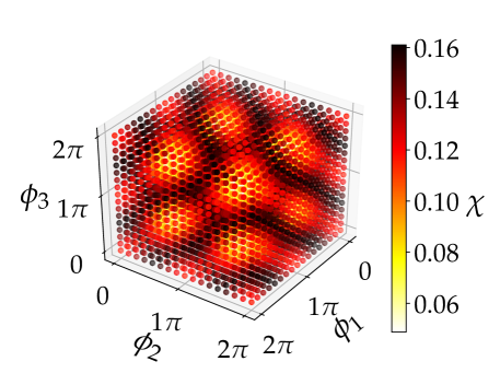
(a)

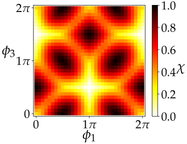
(b)

Figure 4: Performance in the transmission of a single particle through a correlated depolarising channel. (a) Classical capacity in the lack of correlations. Without loss of generality, $\phi_{0}=0$. The maximum capacity is $0.016$ bits. (b) Lower bound to the classical capacity achieved with the correlated probability distribution $p(m,n)=\delta_{n,\sigma(m)}/4$, where $\sigma$ is the permutation that exchanges $0$ with $1$, and $2$ with $3$. Without loss of generality, we set $\phi_{0}=\phi_{2}=0$. The maximum lower bound is 1 bit.

III.4 Lower bound to the classical capacity in the presence of correlations

In the correlated case, we do not have a proof that the classical capacity coincides with the Holevo capacity. On top of that, the evaluation of the Holevo capacity generally requires an optimisation over all possible ensembles of $d^{2}$ linearly independent pure states, which is computationally challenging. Here, we circumvent this problem by computing a lower bound to the Holevo capacity, obtained by restricting the optimisation to the set of all orthogonal ensembles, that is, input ensembles consisting of two orthogonal qubit states. In general, this lower bound may not be tight Fuchs (1997); King et al. (2002); Hayashi et al. (2004), but it is nevertheless interesting as it quantifies the maximum performance of a natural set of encoding strategies. Since the Holevo capacity is always a lower bound to the classical capacity, the above lower bound is also a lower bound to the classical capacity.

Here, we evaluate the lower bound for the correlated channel with $p(m,n)=\delta_{n,\sigma(m)}/4$, where $\sigma$ is the permutation that exchanges $0$ with $1$, and $2$ with $3$. This particular choice is interesting because as we have seen in Subsection III.2, it can reach the maximum capacity of 1 bit. We now inspect how the lower bound depends on the phases.

Since the interference term (11) depends only on the differences $\phi_{1}-\phi_{0}$ and $\phi_{3}-\phi_{2}$, we set $\phi_{0}=\phi_{2}=0$ and scan the possible values of $\phi_{1}$ and $\phi_{3}$. For the state of the control system, we choose again $\omega=|+\rangle\langle+|$, as it maximises the Holevo capacity (cf. Lemma 3 in Appendix B). The lower bound to the Holevo capacity is shown in Figure 4b for all values of $\phi_{1}$ and $\phi_{3}$.

Figure 5: A single particle is sent through a superposition of two paths (orange and blue dashed lines), each traversing two independent channels (green and red ovals), each of which exhibits time correlations between successive uses. The green and red dotted lines represent the correlations between the two subsequent uses of the same channel.

IV Communication through multiple time-correlated channels

Time-correlated channels can be used to mimic the use of ordinary quantum channels in a superposition of different causal orders Oreshkov (2019); Chiribella and Kristjánsson (2019). In this section we show that time correlations are a necessary resource for reproducing the benefits of the superposition of orders in quantum communication, and that, in fact, time correlations are an even more powerful resource than the ability to combine channels in a superposition of orders.

IV.1 A network of time-correlated channels

Suppose that two time-correlated channels $\mathcal{R}_{A}$ and $\mathcal{R}_{B}$, each of the form (1), are arranged as in Figure 5, and that a single particle is sent through a superposition of two alternative paths visiting each of the two channels exactly once. When the control system is initialised in the state $\omega$, the overall evolution of the message and the control is described by the effective channel $\mathcal{E}_{\omega}$ defined as

$$\mathcal{E}_{\omega}(\rho)\mathrel{\mathop{\mathchar 58\relax}}=\sum_{m,n,k,l}p_{A}(m,n)p_{B}(k,l)\,W_{mnkl}(\rho\otimes\omega)W_{mnkl}^{\dagger}\,,$$ (15)

with

$$W_{mnkl}\mathrel{\mathop{\mathchar 58\relax}}= V^{(B)}_{l}V^{(A)}_{m}\,e^{i(\phi^{(B)}_{k}+\phi^{(A)}_{n})}\otimes|0\rangle\langle 0|$$

$$+V^{(A)}_{n}V^{(B)}_{k}\,e^{i(\phi^{(A)}_{m}+\phi^{(B)}_{l})}\otimes|1\rangle\langle 1|\,.$$ (16)

Here, $p_{A}(m,n),p_{B}(k,l),\{V^{(A)}_{m}\},\{V^{(B)}_{l}\},\{\phi^{(A)}_{m}\}$, and $\{\phi^{(B)}_{m}\}$ are defined as in Equations (1) and (2). The derivation of Eq.  (15) is provided in Appendix D.

An interesting special case occurs when the probability distributions $p_{A}(m,n)$ and $p_{B}(k,l)$ are perfectly correlated, that is

$$\begin{split}p_{A}(m,n)&=p_{1A}(m)\delta_{mn}\quad\forall m,n\\ p_{B}(k,l)&=p_{1B}(k)\,\delta_{kl}\quad~{}~{}\forall k,l\,,\end{split}$$ (17)

where $p_{1A}(m)$ and $p_{1B}(k)$ are the marginal probability distributions of $p_{A}(m,n)$ and $p_{B}(k,l)$, respectively. Under this condition, the network in Figure 5 reproduces the action of two random unitary channels in a superposition of two alternative orders Chiribella and Kristjánsson (2019).

Mathematically, the operation of putting two quantum channels in a superposition of orders is described by the quantum SWITCH Chiribella et al. (2009a, 2013), a higher-order transformation that takes as inputs two generic channels $\mathcal{A}$ and $\mathcal{B}$ (with $d$-dimensional input and ouput systems) and produces as output a new quantum channel $\mathcal{S}(\mathcal{A},\mathcal{B})$ with Kraus operators

$$S_{mk}\mathrel{\mathop{\mathchar 58\relax}}=A_{m}B_{k}\otimes|0\rangle\langle 0|+B_{k}A_{m}\otimes|1\rangle\langle 1|\,,$$ (18)

where $\{A_{m}\}$ ($\{B_{k}\}$) are Kraus operators of $\mathcal{A}$ ($\mathcal{B}$), and $\{|0\rangle,|1\rangle\}$ is a basis for a control qubit that determines the relative order between $\mathcal{A}$ and $\mathcal{B}$. Notably, the overall channel $\mathcal{S}(\mathcal{A},\mathcal{B})$ is independent of the choice of Kraus representations for the input channels $\mathcal{A}$ and $\mathcal{B}$.

When the control qubit is put in a fixed state $\omega$, the quantum SWITCH of channels $\mathcal{A}$ and $\mathcal{B}$ yields the effective channel

$$\mathcal{S}_{\omega}(\rho) \mathrel{\mathop{\mathchar 58\relax}}=\sum_{m,k}S_{mk}(\rho\otimes\omega)S_{mk}^{\dagger}\,,$$ (19)

with $S_{mk}$ as in Eq. (18). In particular, here we are interested in the case where the channels $\mathcal{A}$ and $\mathcal{B}$ are random unitary, with Kraus operators $A_{m}\mathrel{\mathop{\mathchar 58\relax}}=\sqrt{p_{1A}(m)}\,V^{(A)}_{m}$ and $B_{k}\mathrel{\mathop{\mathchar 58\relax}}=\sqrt{p_{1B}}\,V^{(B)}_{k}$. With this choice, the channel $\mathcal{S}_{\omega}$ in Eq. (19) coincides with the channel $\mathcal{E}_{\omega}$ in Eq.  (15) under the condition that the probability distributions $p_{A}(m,n)$ and $p_{B}(k,l)$ are perfectly correlated (cf. Eq.  (17)).

When the channels $\mathcal{A}$ and $\mathcal{B}$ are completely depolarising, Ref. Ebler et al. (2018) showed that the channel $\mathcal{S}_{\omega}$ resulting from the quantum SWITCH can transmit $0.049$ bits of classical information, provided that the control is initialised in the state $\omega=|+\rangle\langle+|$. Later, the value $0.049$ was proven to be exactly equal to the classical capacity Chiribella et al. (2020). Since the channels $\mathcal{E}_{\omega}$ and $\mathcal{S}_{\omega}$ coincide, we conclude that the time-correlated network in Figure 5 can achieve a capacity of $0.049$ bits.

In the following, we provide two new results:

1. We show that time correlations are strictly necessary in order to achieve the quantum SWITCH capacity of 0.049 bits. Specifically, we show numerically that the maximum classical capacity in the uncorrelated case is 0.018 bits for random-unitary realisations of the completely depolarising channel, and 0.024 bits for arbitrary realisations. This result shows that, when the quantum SWITCH is reproduced by the network in Figure 5, the origin of the communication enhancement is not just the interference of paths, but rather the combined effect of the interference of paths and of the time correlations.

2. We show that there exist time correlations that achieve a classical capacity of at least $0.31$ bits. This result shows that the access to time correlations is generally a stronger resource than the ability to combine ordinary channels in a superposition of orders.

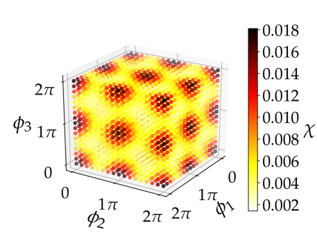
(a)

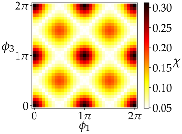
(b)

Figure 6: Performance in the transmission of a single particle through a network of correlated depolarising channels, arranged as in Figure 5. (a) Classical capacity in the lack of correlations. Without loss of generality, $\phi_{0}=0$. The maximum capacity is $0.018$ bits. (b) Lower bound to the classical capacity achieved with maximal correlations corresponding to the probability distributions $p_{A}(m,n)=p_{B}(m,n)=\delta_{n,\sigma(m)}/4$, where $\sigma$ is the permutation that exchanges 0 with 1, and 2 with 3. Without loss of generality, $\phi_{0}=\phi_{2}=0$. The maximum lower bound is $0.31$ bits.

IV.2 Maximum capacity in the lack of correlations

Here we evaluate the maximum amount of classical information that can be transmitted through the network in Figure 5 when the channels are completely depolarising and no correlation is present, that is, when $p_{A}(m,n)=p_{B}(k,l)=1/16~{}\forall m,n,k,l\in\{0,1,2,3\}$.

The evaluation of the maximum capacity follows the same steps as in Subsection III.3. The main observations are:

1. in the lack of correlations, the channel $\mathcal{E}_{\omega}$ in Eq. (15) is entanglement-breaking, and therefore its classical capacity coincides with the Holevo capacity

2. the control state $\omega$ that maximises the Holevo capacity of the channel $\mathcal{E}_{\omega}$ is $\omega=|+\rangle\langle+|$

3. without loss of generality, the maximisation of the Holevo information can be reduced to ensembles that depend only on three real paramters $q,p_{0}$, and $p_{1}$ in $[0,1]$.

The derivation of these results is provided in Appendix E.

Building on the above observations, we evaluate the capacity of the channel $\mathcal{E}_{\omega}$ in Eq. (15) by scanning all possible values of the phases $\{\phi_{m}\}_{m=0}^{3}$. The result is the plot shown in Figure 6a. The largest classical capacity over all random unitary realisations is 0.018 bits, which is strictly smaller than the value $0.049$ bits achieved by the superposition of orders.

Furthermore, we also extend the optimisation from random unitary realisations to arbitrary realisations of the completely depolarising channel. For this broader class of realisations, we numerically obtain that the maximum capacity is $0.024$ bits.

Summarising, the best classical capacity one can obtain by sending a single particle through the network in Figure 5, in the lack of correlations between the two paths, is $0.018$ bits, and the capacity can be increased to $0.024$ bits by replacing the random unitary channels with more general realisations of the completely depolarising channel.

Note that both values $0.018$ and $0.024$ are below the 0.049 bits of classical capacity achieved by the quantum SWITCH. This result shows that, when the quantum SWITCH is reproduced by the correlated network in Figure 5, it offers a communication advantage over all communication protocols where a single particle travels in a superposition of two paths on which it experiences uncorrelated noisy processes. Hence, we conclude that, in this scenario, the origin of the communication advantages of the quantum SWITCH is not merely the superposition of paths, but rather the non-trivial interplay between the superposition of paths and the time correlations in the noise.

Our results also imply a caveat about terminology. The quantum SWITCH of two channels $\mathcal{A}$ and $\mathcal{B}$ is sometimes described informally as a “superposition of channels $\mathcal{A}\mathcal{B}$ and $\mathcal{B}\mathcal{A}$.” While this expression may be formally correct (at least according to a broad notion of superposition Chiribella and Kristjánsson (2019)), it can be misleading if taken at face value, because it does not mention explicitly the requirement of correlations between the channels $\mathcal{A}$ and $\mathcal{B}$ in the two branches of the superposition.

IV.3 Time correlations surpassing the quantum SWITCH capacity

We now show that the classical capacity of $0.049$ bits, achieved by the quantum SWITCH, can be surpassed using more general time correlations. We prove this result explicitly, by exhibiting a pair of time-correlated channels that achieve a capacity at least $0.31$ bits.

Our choice of channels corresponds to $p_{A}(m,n)=p_{B}(m,n)=\delta_{n,\sigma(m)}/4$, where $\sigma$ is the permutation that exchanges $0$ with 1, and 2 with 3. This choice is motivated by the fact that the permutation $\sigma$ guarantees the maximum communication capacity in the case where a single time-correlated channel is used (cf. Subsection III.2).

With the above choice, the effective channel describing the transmission of the message is

$$\mathcal{E}_{\omega}(\rho)=\frac{\frac{I}{2}+\mathcal{K}(\rho)}{2}\otimes\omega+\frac{\frac{I}{2}-\mathcal{K}(\rho)}{2}\otimes Z\omega Z\,,$$ (20)

with

$$\mathcal{K}(\rho)\mathrel{\mathop{\mathchar 58\relax}}=\frac{1}{8}\!\left\{\!\left[\cos 2(\phi_{1}-\phi_{0})+\cos 2(\phi_{3}-\phi_{2})\right]\rho+\!2X\rho X\!\right\}.$$ (21)

The derivation of this formula is provided in Appendix D. Note that the channel $\mathcal{E}_{\omega}$ depends only on the phase differences $\phi_{1}\!-\!\phi_{0}$ and $\phi_{3}\!-\!\phi_{2}$, via Eq. (21).

We now provide a lower bound to the classical capacity of the channel $\mathcal{E}_{\omega}$. As we did earlier in the paper, we lower bound the classical capacity by the Holevo capacity, and, in turn, we lower bound the Holevo capacity by restricting the maximisation to orthogonal input ensembles. For the state of the control qubit, we pick $\omega=|+\rangle\langle+|$, which is the choice that maximises the Holevo capacity (cf. Lemma 3 in Appendix B).

The lower bound to the classical capacity is shown in Figure 6b for all possible values of the phase differences $\phi_{1}\!-\!\phi_{0}$ and $\phi_{3}\!-\!\phi_{2}$. The highest lower bound over all combinations of phases $\{\phi_{m}\}_{m=0}^{3}$ is given by $0.31$ bits. This value is larger than the classical capacity of 0.049 bits achieved by the quantum SWITCH, corresponding to perfect correlations $p_{A}(m,n)=p_{B}(m,n)=\delta_{m,n}/4$. This result implies that not only can time correlations reproduce the superposition of causal orders, but they can also surpass its advantages.

V Noise on the control degree of freedom

So far we have assumed that the message-carrying degree of freedom of the particle undergoes noise during transmission, while the control degree of freedom is noiseless. However, in practical scenarios, this will only be an approximation to the actual physics. We now briefly discuss the effect of noise on the control system, focussing in particular on dephasing noise, of the form

$$\mathcal{P}(\omega)=sZ\omega Z+(1-s)\omega\,,$$ (22)

where $s\in~{}[0,1/2]$ is a probability and $\omega$ is the initial state of the control. For a more detailed investigation into the effects of noise on the control system, we refer the reader to a recent related work Kristjánsson et al. .

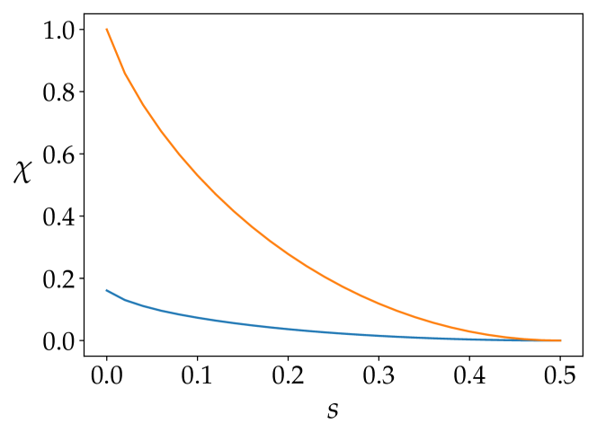
Figure 7: Blue: Maximum classical capacity in the absence of correlations, as a function of the dephasing parameter $s$. The maximum is computed over all realisations of the completely depolarising channel, and is achieved by the random unitary realisation with the choice of phases $\{\phi_{m}\}$ that give the maximum capacity of 0.16 bits when $s=0$. Orange: Lower bound to the maximal classical capacity in the presence of correlations, as a function of the dephasing parameter $s$. The lower bound is computed by considering the correlated probability distribution $p(m,n)=\delta_{n,\sigma(m)}/4$, where $\sigma$ is the permutation that exchanges $0$ with $1$, and $2$ with $3$, and $\phi_{0}=\phi_{1}=\phi_{2}=0,\phi_{3}=\pi/2$.

For simplicity, here we focus on the communication scenario involving a single transmission line, as in Figure 1. In this setting, the evolution experienced by a single particle is described by the channel

$$\mathcal{C}_{\omega}^{\prime}\mathrel{\mathop{\mathchar 58\relax}}=(\mathcal{I}_{M}\otimes\mathcal{P})\mathcal{C}_{\omega}\,,$$ (23)

obtained by dephasing the control system at the output of the channel $\mathcal{C}_{\omega}$ in Eq.  (5). By inserting the expression (5) into the above equation, it is immediate to see that the effect of dephasing is to dampen the interference term $\mathcal{G}$ in the effective channel (5): specifically, the interference term changes from $\mathcal{G}$ to $(1-2s)\,\mathcal{G}$.

In the case of completely depolarising channels on the message degree of freedom, the presence of a non-zero interference term means that, as long as the dephasing of the control is not complete ($s\not=1/2$), the superposition of evolutions can still allow for a non-zero amount of classical information to be transmitted, thereby offering an advantage over the transmission at a definite moment of time.

Figure 7 shows the behaviour of the classical capacity as a function of the dephasing parameter $s$. The figure shows that correlations between two uses of the channel offer an enhancement of the classical capacity. To make this point, we first evaluate numerically the maximum capacity achievable in the lack of correlations, with arbitrary realisations of the completely depolarising channel (blue curve). Notably, the capacity for every fixed value of $s$ is achieved by the same realisation of the completely depolarising channel that achieves the maximum capacity in the ideal $s=0$ case. We then show that a higher capacity can be achieved with the correlated channel described in Subsection III.2. To this purpose, we numerically evaluate a lower bound to the Holevo capacity (and therefore to classical capacity), obtained by restricting the maximisation to orthogonal input ensembles (orange curve). Note that both the blue and orange curves are above 0 for every non-maximal amount of dephasing ($s\not=1/2$), meaning that the single particle transmission at a coherent superposition of times offers an advantage over the transmission at a definite time.

VI Conclusions

We have shown that a single quantum particle can sense the correlations between noisy processes at different moments of time. By sending the particle at a superposition of different times, one can take advantage of these correlations and boost the communication rate to values that would be impossible if the moment of transmission were a classical, well-defined variable.

An important avenue for future research is the experimental realisation of our protocols, as well as the experimental exploration of their noise robustness to timing errors and decoherence between the two different modes used to create the superposition. On the theoretical side, it is interesting to apply our framework for single-particle communication to more complex scenarios, e.g. involving the transmission of a single particle at more than two times, or even in continuous time. It is also interesting to analyse other communication tasks, such as the two-way communication proposed in Ref. Del Santo and Dakić (2018). Moreover, the extension from single particle communication to other communication protocols with a finite number of particles is a natural next step of this research.

At the foundational level, time-correlated channels provide an insight into the resources used by the existing experiments on the superposition of causal order. We analysed a basic setup that reproduces the overall result of the quantum SWITCH by sending a single particle in a superposition of paths through time-correlated channels. In this setup, we showed that time-correlations are a necessary resource to reproduce the communication advantages of the quantum SWITCH. Moreover, we observed that, with more elaborate patterns of correlations, one can achieve an even greater enhancement than the one found for the superposition of orders. This result establishes time-correlated channels as an appealing resource, which can be used as a testbed for foundational results on causal order, and, at the same time, as a building block for new communication protocols.

Appendix A Transmission of a single particle through a superposition of multiple ports

Here we provide a mathematical framework for describing the transmission of a single particle at a superposition of different times, and, more generally, for describing the transmission of the particle on a superposition of different trajectories, each passing through one of the ports of a multiport quantum device.

A.1 Multiport quantum devices and their vacuum extensions

A transmission line with a single input port is described by a quantum channel, that is, a completely positive trace-preserving map transforming density matrices on the particle’s Hilbert space. In the following we will denote by ${\mathsf{Chan}}(S\to S^{\prime})$ the set of quantum channels with input system $S$ and (possibly different) output system $S^{\prime}$. When $S=S^{\prime}$ we will use the shorthand ${\mathsf{Chan}}(S)$. The action of a quantum channel $\mathcal{A}$ on a density matrix $\rho$ can be conveniently written in the Kraus representation $\mathcal{A}\left(\rho\right)=\sum_{i}A_{i}\rho A_{i}^{\dagger}$, where $\left\{A_{i}\right\}$ is a (non-unique) set of operators, satisfying $\sum_{i}A_{i}^{\dagger}A_{i}=I$.

A transmission line with $k$ input/output ports is described by a $k$-partite quantum channel $\mathcal{B}\in{\mathsf{Chan}}\left(S^{(1)}\otimes\cdots\otimes S^{(k)}\to S^{\prime(1)}\otimes\cdots\otimes S^{\prime(k)}\right)$ with $k$ input-output pairs $(S^{(i)},S^{\prime(i)})_{i=1}^{k}$.

Figure 8: The left-hand side depicts a 2-step correlated quantum channel $\mathcal{B}$ taking two input states on systems $S^{(1)}$ and $S^{(2)}$, in succession. The right-hand side shows the physical implementation of the 2-step channel via two unitary channels $\mathcal{W}_{1}$ and $\mathcal{W}_{2}$ Chiribella et al. (2008a, 2009b) where the memory between the two uses of the channel is realised by an environment $E$, which is inaccessible to the communicating parties.

A transmission line that can be used $k$ times in succession is described by $k$-step quantum channel Macchiavello and Palma (2002) (also known as a quantum $k$-comb Chiribella et al. (2008a, 2009b)). A $k$-step quantum channel is a special type of $k$-partite channel $\mathcal{B}$ with the additional property that no signal propagates from an input $S^{(i)}$ to any group of outputs $S^{\prime(j)}$ with $j<i$ Chiribella et al. (2008a). We will denote the set of $k$-step quantum channels as ${\mathsf{Chan}}(S^{(1)}\to S^{\prime(1)},\dots,S^{(k)}\to S^{\prime(k)})$, or simply ${\mathsf{Chan}}(S^{(1)},\dots,S^{(k)})$ when the input and output of each pair coincide. For $k=2$, an example of 2-step quantum channel is illustrated in Figure 8.

The possibility that no particle is sent through a port of a device can be described using the notion of vacuum extension Chiribella and Kristjánsson (2019). Consider first a single-port device, described by an ordinary quantum channel $\mathcal{A}\in{\mathsf{Chan}}(S)$. When no particle is sent through the device, we describe the input as the vacuum state $\ket{\textrm{vac}}$, that is, a state in a vacuum sector Vac Åberg (2004b); Zhou et al. (2011); Chiribella and Kristjánsson (2019); Dong et al. (2019), which is orthogonal to the one-particle sector $S$. Overall, the device acts on an extended system $\widetilde{S}\mathrel{\mathop{\mathchar 58\relax}}=S\oplus\textrm{Vac}$, which is associated with the Hilbert space given by $\mathcal{H}_{S}\oplus\mathcal{H}_{\rm Vac}$, where $\mathcal{H}_{\rm Vac}$ is the vacuum Hilbert space, here assumed to be one-dimensional.

Given a quantum channel $\mathcal{A}$, a vacuum extension $\widetilde{\mathcal{A}}$ of $\mathcal{A}$ is any channel which acts as $\mathcal{A}$ (respectively, $\mathcal{I}_{\textrm{Vac}}$) when the input is a state in sector $S$ (respectively, Vac). The Kraus operators of $\widetilde{\mathcal{A}}$ are $\widetilde{A}_{i}=A_{i}\oplus\alpha_{i}\,|\rm vac\rangle\langle\rm vac|$, where $\{A_{i}\}_{i=0}^{r-1}$ is a Kraus representation of $\mathcal{A}$, and $\{\alpha_{i}\}_{i=0}^{r-1}$ are vacuum amplitudes satisfying $\sum_{i=0}^{r-1}\,|\alpha_{i}|^{2}=1$.

A given channel has infinitely many possible vacuum extensions. In an actual communication scenario, the vacuum extension can be determined by probing the action of the channel on superpositions of the vacuum and one-particle states. Physically, the choice of vacuum extension is determined by the Hamiltonian of the field describing the vacuum and the one-particle sector.

The notion of vacuum extension can be easily extended to the case of $k$-partite channels, which include $k$-step channels as a special case. For simplicity, we focus on the $k=2$ case, but the extension to $k\geq 2$ is straightforward.

Consider a transmission line described by a bipartite channel $\mathcal{B}\in{\mathsf{Chan}}(S^{(1)}\otimes S^{(2)})$. A vacuum extension of the channel $\mathcal{B}$ is another bipartite channel $\widetilde{\mathcal{B}}\in{\mathsf{Chan}}(\widetilde{S}^{(1)}\otimes\widetilde{S}^{(2)})$, acting on the extended systems $\widetilde{S}^{(1)}\mathrel{\mathop{\mathchar 58\relax}}=S^{(1)}\oplus{\rm Vac}^{(1)}$ and $\widetilde{S}^{(2)}\mathrel{\mathop{\mathchar 58\relax}}=S^{(2)}\oplus{\rm Vac}^{(2)}$. In general, the systems $S^{(1)},S^{(2)}$ can represent the systems accessible at the same location at two consecutive moment of time, or it can represent the systems accessible at different locations at the same time (as considered in Refs. Abbott et al. (2020); Chiribella and Kristjánsson (2019)), or more generally, they can represent any pair of independently aderressable systems, representing the input/output ports of our multiport device.

A.2 A single particle travelling through multiple ports

In order to be able to send the same quantum particle to either of the ports of the device, we require the isomorphism $S^{(1)}\cong S^{(2)}\cong M$, where $M$ is the message-carrying degree of freedom of the particle. In this case, the tensor product $\widetilde{S}^{(1)}\otimes\widetilde{S}^{(2)}$ contains a no-particle sector ${\rm Vac}^{(1)}\otimes{\rm Vac}^{(2)}$, a one-particle sector $(S^{(1)}\otimes{\rm Vac}^{(2)})\oplus({\rm Vac}^{(1)}\otimes S^{(2)})$, and a two-particle sector $S^{(1)}\otimes S^{(2)}$. The one-particle sector is isomorphic to $M\otimes C$, where $C$ is a qubit system, representing the degree of freedom of the particle that controls its time of transmission. When the control is in state $\ket{0}$, the message is sent through the first application of the channel and the vacuum is sent in the second application; vice versa for the control in state $\ket{1}$.

We now define the situation in which a single particle is sent at a superposition of two different ports. We call the process experienced by the particle the superposition channel $\mathcal{S}(\widetilde{\mathcal{B}})$, and define it as the restriction of $\widetilde{\mathcal{B}}$ to the one-particle sector, regarded as isomorphic to the composite system “message + control.” Explicitly, the action of the superposition channel is defined as

$$\mathcal{S}(\widetilde{\mathcal{B}})\mathrel{\mathop{\mathchar 58\relax}}=\mathcal{U}^{\dagger}\circ\widetilde{\mathcal{B}}\circ\mathcal{U}\,,$$ (24)

where $\mathcal{U}(\cdot)\mathrel{\mathop{\mathchar 58\relax}}=U(\cdot)U^{\dagger}$ is the isomorphism between $M\otimes C$ and the one-particle sector $(S^{(1)}\otimes{\rm Vac})\oplus({\rm Vac}\otimes S^{(2)})$, with

$$U(|\psi\rangle_{M}\otimes|0\rangle_{C}) \mathrel{\mathop{\mathchar 58\relax}}=|\psi\rangle_{\widetilde{S}^{(1)}}\otimes|{\rm vac}\rangle_{\widetilde{S}^{(2)}}$$

$$U(|\psi\rangle_{M}\otimes|1\rangle_{C}) \mathrel{\mathop{\mathchar 58\relax}}=|{\rm vac}\rangle_{\widetilde{S}^{(1)}}\otimes|\psi\rangle_{\widetilde{S}^{(2)}}\,.$$ (25)

Mathematically, the transformation $\mathcal{S}\mathrel{\mathop{\mathchar 58\relax}}{\mathsf{Chan}}(\widetilde{S}^{(1)}\otimes\widetilde{S}^{(2)})\rightarrow{\mathsf{Chan}}(M\otimes C)$ is a quantum supermap, that is, a transformation from quantum channels to quantum channels satisfying appropriate consistency requirements Chiribella et al. (2008b, 2009b, 2013). An illustration of the supermap $\mathcal{S}$ is provided in subfigure 9a.

Note that definition (24) can be applied in particular to $k$-step quantum channels, which are a special case of $k$-partite channels. The illustration of the supermap $\mathcal{S}$ in this special case is provided in subfigure 9b.

The same definition can be adopted for the transmission of a single particle through a $k$-partite multiport device. In this case, the device is represented by a $k$-partite quantum channel $\mathcal{B}\in{\mathsf{Chan}}(S^{(1)}\otimes\dots\otimes S^{(k)})$, with $S^{(1)}\cong S^{(2)}\cong\cdots\cong S^{(k)}$, and with vacuum extension $\widetilde{\mathcal{B}}\in{\mathsf{Chan}}(\widetilde{S}^{(1)}\otimes\dots\otimes\widetilde{S}^{(k)})$. The superposition channel is then defined as the restriction of $\widetilde{\mathcal{B}}$ to the one-particle sector

$$\bigoplus_{j=1}^{k}{\rm Vac}^{(1)}\!\otimes\!\cdots\!\otimes\!{\rm Vac}^{(j-1)}\otimes S^{(j)}\otimes\!{\rm Vac}^{(j+1)}\!\otimes\!\cdots\!\otimes\!{\rm Vac}^{(k)}$$

$$\qquad\qquad\qquad\cong M\otimes C\,,$$ (26)

where $C$ is now a $k$-dimensional control system.

(a)

(b)

Figure 9: (a) Transmission of a single particle through a bipartite quantum channel $\widetilde{\mathcal{B}}$ (green). (b) Transmission of a single particle through a 2-step quantum channel $\widetilde{\mathcal{B}}$ (green). In both caes, the particle is represented by a composite system $M\otimes C$, where $M$ represents the degrees of freedom used as the message, and $C$ represents the degrees of freedom used as the control. The isomorphism $\mathcal{U}$ converts the composite system $M\otimes C$ into the one-particle sector $(S^{(1)}\otimes{\rm Vac})\oplus({\rm Vac}\otimes S^{(2)})$ of $\widetilde{S}^{(1)}\otimes\widetilde{S}^{(2)}$. The inverse map $\mathcal{U}^{\dagger}$ converts the output state back into $M\otimes C$. For the applications in this paper, we take the input of the control system $C$ to be fixed in the state $\omega$ whilst the message system $M$ is accessible to the sender.

A.3 Derivation of Eq. (4) in the main text

We now specialise to the case of correlated channels of the random unitary form

$$\mathcal{R}=\sum_{m,n}p(m,n)\,\mathcal{V}_{m}\otimes\mathcal{V}_{n}\in{\mathsf{Chan}}(S^{(1)},S^{(2)})\,,$$ (27)

where $\mathcal{V}_{m}(\cdot)\mathrel{\mathop{\mathchar 58\relax}}=V_{m}(\cdot)V_{m}^{\dagger}$ is a unitary channel, $\{V_{m}\}$ is a set of unitary gates, and $p(m,n)$ is a joint probability distribution. The vacuum extension of each unitary $V_{m}$ is taken to be another unitary $U_{m}$, which we write as

$$\widetilde{V}_{m}\mathrel{\mathop{\mathchar 58\relax}}=U_{m}=V_{m}\oplus e^{i\phi_{m}}\ket{\rm vac}\!\bra{\rm vac}\,,$$ (28)

where the vacuum amplitude is given by a complex phase, representing the coherent action of each possible noisy process on the one-particle and vacuum sectors. This leads to the vacuum extension

$$\widetilde{\mathcal{R}}=\sum_{m,n}p(m,n)\,\widetilde{\mathcal{V}}_{m},\widetilde{\mathcal{V}}_{n}\in{\mathsf{Chan}}(\widetilde{S}^{(1)},\widetilde{S}^{(2)})\,,$$ (29)

with $\widetilde{\mathcal{V}}_{m}(\cdot)\mathrel{\mathop{\mathchar 58\relax}}=\widetilde{V}_{m}(\cdot)\widetilde{V}_{m}^{\dagger}$, which is equivalent to Equation (1) in the main text, with $U_{m}=\widetilde{V}_{m}$.

The use of the channel $\mathcal{R}$, specified by the vacuum extension $\widetilde{\mathcal{R}}$, at a superposition of times is given by:

$$\mathcal{S}(\widetilde{\mathcal{R}})=\!\!\sum_{m,n=0}^{r-1}p(m,n)\,\mathcal{U}^{\dagger}\!\circ\!\left(\widetilde{\mathcal{V}}_{m}\otimes\widetilde{\mathcal{V}}_{n}\right)\!\circ\mathcal{U}\,.$$ (30)

Explicitly, we have the expression

$$\mathcal{S}(\widetilde{\mathcal{R}})(\rho\otimes\omega)=\sum_{m,n}C_{mn}\,(\rho\otimes\omega)\,C_{mn}^{\dagger}\,,$$ (31)

where $\rho$ (respectively, $\omega$) is an arbitrary state of the message (respectively, control), and

$$C_{mn} \mathrel{\mathop{\mathchar 58\relax}}=\sqrt{p(m,n)}e^{i\phi_{n}}V_{m}\,\otimes|0\rangle\langle 0|$$

$$~{}~{}+\sqrt{p(m,n)}V_{n}e^{i\phi_{m}}\,\otimes|1\rangle\langle 1|\,,$$ (32)

$e^{i\phi_{m}}$ being the vacuum amplitude in Eq. (28). Eq. (31) coincides with Equation (4) in the main text, with $\mathcal{C}\mathrel{\mathop{\mathchar 58\relax}}=\mathcal{S}(\widetilde{\mathcal{R}})$ and $W_{mn}\mathrel{\mathop{\mathchar 58\relax}}=C_{mn}/\sqrt{p(m,n)}$.

A.4 Derivation of Eq. (5)–(7) in the main text

It is useful to consider the case where the probability distribution $p(m,n)$ is symmetric, that is, $p(m,n)=p(n,m)$ for every $m$ and $n$. In this case, the superposition channel has the simple expression

$$\mathcal{S}(\widetilde{\mathcal{R}})=\frac{\mathcal{R}_{1}+\mathcal{G}}{2}\otimes\mathcal{I}+\frac{\mathcal{R}_{1}-\mathcal{G}}{2}\otimes\mathcal{Z}\,,$$ (33)

where $\mathcal{Z}$ is the unitary channel associated to the Pauli matrix $Z$, $\mathcal{R}_{1}$ is the reduced channel defined by

$$\mathcal{R}_{1}(\rho)\mathrel{\mathop{\mathchar 58\relax}}=\sum_{m}\,p_{1}(m)\,V_{m}\rho V_{m}^{\dagger}\qquad p_{1}(m)\mathrel{\mathop{\mathchar 58\relax}}=\sum_{n}\,p(m,n)\,,$$ (34)

and $\mathcal{G}$ is the linear map defined by

$$\mathcal{G}(\rho)\mathrel{\mathop{\mathchar 58\relax}}=\sum_{m,n}\,p(m,n)~{}e^{i(\phi_{n}-\phi_{m})}\,V_{m}\rho V_{n}^{\dagger}\,.$$ (35)

Appendix B Analytical bound on the classical capacity in the lack of correlations

This section refers to the scenario where the message is transmitted at a superposition of two possible times, experiencing independent noisy processes that are completely depolarising in the one-particle subspace. This section makes use of the notation introduced in Appendix A.

B.1 Proof that the superposition of uncorrelated completely depolarising channels is entanglement-breaking

Let $\mathcal{A}(\cdot)=\sum_{m=0}^{r-1}A_{m}(\cdot)A_{m}^{\dagger}\in{\mathsf{Chan}}(S)$ be a generic quantum channel, and let $\widetilde{\mathcal{A}}\in{\mathsf{Chan}}(\widetilde{S})$ be a vacuum extension of $\mathcal{A}$. Using Eq. (24), we obtain

$$\mathcal{S} (\widetilde{\mathcal{A}}\otimes\widetilde{\mathcal{A}})$$

$$=\frac{\mathcal{A}\left(\rho\right)+F\rho F^{\dagger}}{2}\otimes\mathcal{I}+\frac{\mathcal{A}\left(\rho\right)-F\rho F^{\dagger}}{2}\otimes\mathcal{Z}\,,$$ (36)

where $\mathcal{I}$ (respectively, $\mathcal{Z}$) is the identity channel (respectively, Pauli channel corresponding to the Pauli matrix $Z$), and

$$F\mathrel{\mathop{\mathchar 58\relax}}=\sum_{m}\,\overline{\alpha}_{m}\,A_{m}$$ (37)

is the vacuum interference operator defined in Ref. Chiribella and Kristjánsson (2019).

Now, let $\mathcal{A}$ be the completely depolarising channel $\mathcal{D}\mathrel{\mathop{\mathchar 58\relax}}\rho\mapsto I/d$, with vacuum extension $\widetilde{\mathcal{D}}$. For a fixed state $\omega$ of the control system, consider the effective channel defined by

$$\mathcal{S}(\widetilde{\mathcal{D}}\!\otimes\!\widetilde{\mathcal{D}})(\rho\otimes\omega) =\frac{I/d+F\rho F^{\dagger}}{2}\otimes\mathcal{I}+\frac{I/d-F\rho F^{\dagger}}{2}\otimes\mathcal{Z}$$

$$=\mathrel{\mathop{\mathchar 58\relax}}\mathcal{C}_{\omega,F}(\rho)\,.$$ (38)

For $d=2$, we have the following result:

Proposition 1.

The channel $\mathcal{C}_{\omega,F}$ in Eq. (38) is entanglement-breaking for $d=2$.

The proof uses the following lemma:

Lemma 2.

Let $\mathcal{D}$ be a completely depolarising channel with vacuum extension $\widetilde{\mathcal{D}}$ and vacuum interference operator $F$. Then, the operator norm of $F$ satisfies the inequality $||F||_{\infty}\leq\frac{1}{\sqrt{d}}$.

Proof.  Let the Kraus operators and vacuum amplitudes of $\mathcal{D}$ be given by $\{A_{i}\},\{\alpha_{i}\}$, respectively. By definition,

$$||F||_{\infty}=\max_{\{|v\rangle\mathrel{\mathop{\mathchar 58\relax}}|||v\rangle||=1\}}~{}\max_{\{|w\rangle\mathrel{\mathop{\mathchar 58\relax}}|||w\rangle||=1\}}\langle v|F|w\rangle$$ (39)

and

$$\begin{split}\left|\langle v|F|w\rangle\right|&=\left|\sum_{i}\overline{\alpha_{i}}\langle v|A_{i}|w\rangle\right|\\ &\leq\sqrt{\left(\sum_{i}|\alpha_{i}|^{2}\right)\left(\sum_{j}\langle v|A_{j}|w\rangle\langle w|A_{j}^{\dagger}|v\rangle\right)}\\ &=\sqrt{\langle v|\mathcal{D}\left(|w\rangle\langle w|\right)|v\rangle}\end{split}$$ (40)

If $\mathcal{D}$ is the completely depolarising channel, then $\mathcal{D}(|w\rangle\langle w|)=I/d$ and therefore the bound becomes $|\langle v|F|w\rangle|\leq\sqrt{1/d}$ which implies $||F||_{\infty}\leq\sqrt{1/d}$. ∎

We are now ready to provide the proof of Proposition 1.

Proof of Proposition 1. To prove that a channel is entanglement-breaking, it is sufficient show that it transforms a maximally entangled state into a separable state Horodecki et al. (2003). Let $|\Phi^{+}\rangle=\sum_{k=0}^{d-1}\,|k\rangle\otimes|k\rangle/\sqrt{d}$ be the canonical maximally entangled state. When the channel $\mathcal{C}_{\omega,F}$ is applied, the output state is

$$(\mathcal{C}_{\omega,F}\otimes\mathcal{I})(|\Phi^{+}\rangle\langle\Phi^{+}|)= \left(\frac{I\otimes I}{d^{2}}+G_{F}\right)\otimes\frac{\omega}{2}$$

$$+\left(\frac{I\otimes I}{d^{2}}-G_{F}\right)\otimes\frac{Z\omega Z}{2}\,,$$ (41)

with $G_{F}\mathrel{\mathop{\mathchar 58\relax}}=(F\otimes I)(|\Phi^{+}\rangle\langle\Phi^{+}|)(F\otimes I)^{\dagger}$.

We now show that the operators $\frac{I\otimes I}{d^{2}}\pm G_{F}$ are proportional to states with positive partial transpose. To this purpose, note that the partial transpose of $G_{F}$ on the second space is

$$G_{F}^{\tau_{2}}=(F\otimes I)\frac{{\tt SWAP}}{d}(F\otimes I)^{\dagger}\,.$$ (42)

Hence, for every unit vector $|\Psi\rangle$ we have the bound,

$$\langle\Psi|G_{F}^{\tau_{2}}|\Psi\rangle \leq\frac{\langle\Psi|(FF^{\dagger}\otimes I)|\Psi\rangle}{d}$$

$$\leq\frac{\|FF^{\dagger}\|_{\infty}}{d}$$

$$=\frac{\|F\|_{\infty}^{2}}{d}$$

$$\leq\frac{1}{d^{2}}\,.$$ (43)

where the first inequality follows from Schwarz’ inequality, and the last inequality follows from Lemma 2.

Using Eq. (43), we obtain the relation

$$\langle\Psi|\left(\frac{I\otimes I}{d^{2}}\pm G_{F}\right)^{\tau_{2}}\,|\Psi\rangle\geq\frac{1}{d^{2}}-\langle\Psi|G_{F}^{\tau_{2}}|\Psi\rangle\geq 0\,.$$ (44)

Since $|\Psi\rangle$ is an arbitrary vector, we conclude that the operator $\left(\frac{I\otimes I}{d^{2}}\pm G_{F}\right)^{\tau_{2}}$ has positive partial transpose. For $d=2$, the Peres-Horodecki criterion Peres (1996); Horodecki et al. (2001), guarantees that $\frac{I\otimes I}{4}\pm G_{F}$ is proportional to a separable state. Hence, the whole output state (41) is separable. ∎

B.2 Optimal control state for maximizing the Holevo capacity

Proposition 1 implies that the classical capacity of the channel $\mathcal{C}_{\omega,F}$ is equal to its Holevo capacity (see Shor (2002)). Here we show that the Holevo capacity is maximised by the state $\omega=|+\rangle\langle+|$. In fact, we prove a more general result:

Lemma 3.

Let $\mathcal{C}_{\omega}$ be an arbitrary channel of the form

$$\mathcal{C}_{\omega}(\rho)\mathrel{\mathop{\mathchar 58\relax}}=\mathcal{L}_{+}(\rho)\otimes\omega+\mathcal{L}_{-}(\rho)\otimes Z\omega Z\,,$$ (45)

where $\mathcal{L}_{\pm}$ are arbitrary linear maps. Then, for every density matrix $\omega$, the Holevo capacity satisfies the bound $\chi\left(\mathcal{C}_{\omega}\right)\leq\chi\left(\mathcal{C}_{|+\rangle\langle+|}\right)$.

Proof.  The Holevo capacity is known to be monotonically decreasing under the adtion of quantum channels, namely $\chi(\mathcal{E})\geq\chi(\mathcal{F}\circ\mathcal{E})$ for every pair of channels $\mathcal{E}$ and $\mathcal{F}$. For every channel $\mathcal{C}_{\omega}$ of the form (45), we have the relation

$$\mathcal{C}_{\omega}=(\mathcal{I}_{M}\otimes\mathcal{P}_{\omega})\circ\mathcal{C}_{|+\rangle\langle+|}\,,$$ (46)

where $\mathcal{P}_{\omega}$ is the quantum channel defined by

$$\mathcal{P}_{\omega}(\gamma)\mathrel{\mathop{\mathchar 58\relax}}=\langle+|\gamma|+\rangle\,\omega+\langle-|\gamma|-\rangle\,Z\omega Z$$ (47)

for an arbitrary state $\gamma$. Hence, we have $\chi(\mathcal{C}_{\omega})=\chi\left[(\mathcal{I}_{M}\otimes\mathcal{P}_{\omega})\circ\mathcal{C}_{|+\rangle\langle+|}\right]\leq\chi(\mathcal{C}_{|+\rangle\langle+|})$. ∎

Lemma 3 holds in particular for

1. the channel $\mathcal{C}_{\omega,F}$ defined in Eq. (38)

2. the channel $\mathcal{C}_{\omega}$ defined in Eq. (9) of the main text

3. the channel $\mathcal{E}_{\omega,F}$ defined in Eq. (20) of the main text.

B.3 Bound on the Holevo capacity

Proposition 4.

The Holevo capacity of the channel $\mathcal{C}_{\omega,F}$ defined in Eq. (38) is upper bounded as

$$\begin{split}\chi(\mathcal{C}_{\omega,F})\leq\frac{\log(2d)}{d}&+\frac{\frac{1}{d}+||F||_{\infty}^{~{}2}}{2}\log\frac{\frac{1}{d}+||F||_{\infty}^{~{}2}}{2}\\ &+\frac{\frac{1}{d}-||F||_{\infty}^{~{}2}}{2}\log\frac{\frac{1}{d}-||F||_{\infty}^{~{}2}}{2}\,,\end{split}$$ (48)

where $F$ is the vacuum interference operator defined in Eq. (37).

Proof.  For a fixed vacuum extension, and therefore for a fixed vacuum interference operator $F$, the Holevo capacity of the channel $\mathcal{C}_{\omega}$ is upper bounded by the Holevo capacity of the channel $\mathcal{C}_{|+\rangle\langle+|,F}$ (Lemma 3). Hence, it is enough to prove the bound for the channel $\mathcal{C}_{|+\rangle\langle+|}$.

Note that the output of channel $\mathcal{C}_{|+\rangle\langle+|,F}$ has dimension $2d$. For a generic channel $\mathcal{E}$ with $(2d)$-dimensional output, the Holevo capacity is upper bounded as Holevo (2002)

$$\chi(\mathcal{E})\leq\log(2d)-\min_{\rho}H\left[\mathcal{E}(\rho)\right]\,,$$ (49)

where $H(\rho)\mathrel{\mathop{\mathchar 58\relax}}=-\operatorname{Tr}[\rho\log\rho]$ is the von Neumann entropy, and the minimisation can be restricted without loss of generality to pure states.

We now upper bound the right-hand-side of Eq. (49) for $\mathcal{E}=\mathcal{C}_{|+\rangle\langle+|,F}$. The action of the channel $\mathcal{C}_{|+\rangle\langle+|,F}$ on a generic input state $\rho$ is

$$\mathcal{C}_{|+\rangle\langle+|,F}(\rho)=\frac{\frac{I}{d}\!+\!F\rho F^{\dagger}}{2}\otimes|\!+\!\rangle\langle\!+\!|+\frac{\frac{I}{d}\!-\!F\rho F^{\dagger}}{2}\otimes|\!-\!\rangle\langle\!-\!|\,,$$ (50)

as one can deduce from Eqs. (38) and (B.1).

In the case of a pure state $\rho=|\psi\rangle\langle\psi|$, we write $F|\psi\rangle=k\,|\varphi\rangle$, where $|\varphi\rangle$ is a unit vector and $k$ is a normalisation constant. With this notation, we obtain

$$\begin{split}\mathcal{C}_{|+\rangle\langle+|,F}(|\psi\rangle\langle\psi|)&=\frac{(\frac{1}{d}+k^{2})\ket{\varphi}\!\bra{\varphi}+\frac{1}{d}P_{\perp}}{2}\otimes|+\rangle\langle+|\\ &~{}+\frac{(\frac{1}{d}-k^{2})\ket{\varphi}\!\bra{\varphi}+\frac{1}{d}P_{\perp}}{2}\otimes|-\rangle\langle-|\,,\end{split}$$ (51)

with $P_{\perp}\mathrel{\mathop{\mathchar 58\relax}}=I-|\varphi\rangle\langle\varphi|$. The von Neumann entropy of this state is

$$\begin{split}H&\left[\mathcal{C}_{|+\rangle\langle+|,F}(|\psi\rangle\langle\psi|)\right]\\ &=-\frac{\frac{1}{d}+k^{2}}{2}\log\frac{\frac{1}{d}+k^{2}}{2}-\frac{d-1}{2d}\log\frac{1}{2d}\\ &\quad-\frac{\frac{1}{d}-k^{2}}{2}\log\frac{\frac{1}{d}-k^{2}}{2}-\frac{d-1}{2d}\log\frac{1}{2d}\\ &=\frac{d-1}{d}\log(2d)\\ &\quad-\frac{\frac{1}{d}+k^{2}}{2}\log\frac{\frac{1}{d}+k^{2}}{2}-\frac{\frac{1}{d}-k^{2}}{2}\log\frac{\frac{1}{d}-k^{2}}{2}\end{split}$$ (52)

Now, note that one has

$$k=\|F\,|\psi\rangle\|\leq\|F\|_{\infty}\leq\frac{1}{\sqrt{d}}\,,$$ (53)

where the last inequality follows from Lemma 2. The expression (52) is monotonically decreasing for $k$ in the interval $[0,1/\sqrt{d}]$. Hence, one has the lower bound

$$\begin{split}H\left[\mathcal{C}_{|+\rangle\langle+|,F}(|\psi\rangle\langle\psi|)\right]&\geq\frac{d-1}{d}\log(2d)\\ &\quad-\frac{\frac{1}{d}+\|F\|_{\infty}^{2}}{2}\log\frac{\frac{1}{d}+\|F\|_{\infty}^{2}}{2}\\ &\quad-\frac{\frac{1}{d}-\|F\|_{\infty}^{2}}{2}\log\frac{\frac{1}{d}-\|F\|_{\infty}^{2}}{2}\end{split}\,.$$ (54)

Inserting this expression into Eq.  (49) with $\mathcal{E}=\mathcal{C}_{|+\rangle\langle+|,F}$, we then obtain Eq. (48). ∎

Corollary 5.

The Holevo capacity of the channel $\mathcal{C}_{\omega,F}$ defined in Eq. (38) is upper bounded as $\chi(\mathcal{C}_{\omega,F})\leq 1/d$. In particular, for $d=2$, one has the bound $\chi(\mathcal{C}_{\omega,F})\leq 0.5$.

Proof.  Immediate from the fact that the right-hand-side of Eq. (48) is monotonically decreasing with $\|F\|_{\infty}$, and that $\|F\|_{\infty}$ is upper bounded by $1/\sqrt{d}$ (Lemma 2). ∎

Appendix C Maximisation of the Holevo information for the superposition of independent depolarising channels

Here we prove a series of results that enable a complete numerical maximisation of the Holevo information of the channel (38)

$$\mathcal{C}_{\omega,F}\mathrel{\mathop{\mathchar 58\relax}}\rho\mapsto\frac{I/d+F\rho F^{\dagger}}{2}\otimes\omega+\frac{I/d-F\rho F^{\dagger}}{2}\otimes Z\omega Z$$ (55)

over all input ensembles, over all states of the control system, and over all vacuum extensions of the completely depolarising channel. This Appendix makes use of notation introduced in the previous appendices.

Let us start from the maximisation over the vacuum extensions, which are in one-to-one correspondence with the possible operators $F$.

Lemma 6.

Without loss of generality, the operator $F$ that maximises the Holevo information of the channel $\mathcal{C}_{\omega,F}$ can be taken to be of the form $F=a\,|0\rangle\langle 0|+b|1\rangle\langle 1|$, with $a^{2}+b^{2}\leq 1/d$,  $a,b\geq 0$.

Proof.  Using the singular value decomposition, $F$ can be written as $F=UF^{\prime}V$, where $U$ and $V$ are suitable unitary matrices, and $F^{\prime}$ is diagonal in the basis $\{|0\rangle,|1\rangle\}$. Now the capacity of the channel $\mathcal{C}_{\omega,F}$ is equal to the capacity of the channel $\mathcal{C}_{\omega,F^{\prime}}=(\mathcal{U}\otimes\mathcal{I}_{C})^{\dagger}\circ\mathcal{C}_{\omega,F}\circ\mathcal{V}^{{\dagger}}$, where $\mathcal{U}^{\dagger}$ and $\mathcal{V}^{\dagger}$ are the inverses of the unitary channels associated to the unitary matrices $U$ and $V$, respectively, and $\mathcal{I}_{C}$ is the identity channel on the control system. Notice that $F^{\prime}$ is also a vacuum interference operator associated to the completely depolarising channel. Hence, the maximisation of the Holevo capacity can be restricted to channels with diagonal vacuum interference operator.

Next, we note that, for a vacuum extension of the completely depolarising channel, the vacuum interference operator $F$ must satisfy the condition $\operatorname{Tr}F^{\dagger}F\leq 1/d$ Abbott et al. (2020). For an operator of the form $F=a\,|0\rangle\langle 0|+b\,|1\rangle\langle 1|$, this implies the inequality $|a|^{2}+|b|^{2}\leq 1/d$. Finally, we show that $a,b$ can restricted to positive numbers. Let $W=a^{\prime}\ket{0}\!\bra{0}+b^{\prime}\ket{1}\!\bra{1}$, where $a^{\prime}=\bar{a}/|a|,b^{\prime}=\bar{b}/|b|$. Then $F^{\prime\prime}\mathrel{\mathop{\mathchar 58\relax}}=WF=FW=|a|\ket{0}\!\bra{0}+|b|\ket{1}\!\bra{1}$. The capacity of the channel $\mathcal{C}_{\omega,F^{\prime\prime}}=(\mathcal{W}\otimes\mathcal{I}_{C})\circ\mathcal{C}_{\omega,F}$ (where $\mathcal{W}$ is the unitary channel associated with the unitary $W$) is equal to the capacity of the channel $\mathcal{C}_{\omega,F}$. Therefore, a maximisation of the Holevo capacity can be restricted to vacuum interference operators with positive coefficients in the computational basis. ∎

Let us consider now the maximisation over all possible ensembles. The key result here is that the maximisation can be reduced to the optimisation of $d$ vectors with positive coefficients in the computational basis.

Lemma 7.

When the operator $F$ is diagonal in the computational basis, the input ensemble that maximises the Holevo information after application of the channel $\mathcal{C}_{\omega,F}$ can be chosen without loss of generality to be of the form

$$\left\{\frac{p_{x}}{d},\,M^{j}|\psi_{x}\rangle\langle\psi_{x}|M^{j{\dagger}}\right\}_{x\in\{0,\dots,d-1\},\,j\in\{0,\dots,d-1\}}\,,$$ (56)

where $(p_{x})_{x\in\{0,\dots,d-1\}}$ is a probability distribution, $M$ is the unitary operator $M\mathrel{\mathop{\mathchar 58\relax}}=\sum_{m=0}^{d-1}\,\omega^{m}\,|m\rangle\langle m|$, $\omega\mathrel{\mathop{\mathchar 58\relax}}=e^{2\pi i/d}$, and $|\psi_{x}\rangle$ is a unit vector with positive coefficients in the computational basis $\{|m\rangle\}_{m=0}^{d-1}$.

Proof.  When $F$ is diagonal, the channel $\mathcal{C}_{\omega,F}$ has the covariance property

$$\mathcal{C}_{\omega,F}\circ\mathcal{U}_{\boldsymbol{\theta}}=(\mathcal{U}_{\boldsymbol{\theta}}\otimes\mathcal{I}_{C})\circ\mathcal{C}_{\omega,F}\qquad\,\forall{\boldsymbol{\theta}}\,,$$ (57)

where ${\boldsymbol{\theta}}=(\theta_{0},\theta_{1},\dots,\theta_{d-1})$ is a vector of $d$ phases, and $\mathcal{U}_{\theta}$ is the unitary channel associated to the unitary matrix $U_{\boldsymbol{\theta}}=\sum_{m=0}^{d-1}\,e^{i\theta_{m}}\,|m\rangle\langle m|$. Note that, in particular, we have

$$\mathcal{C}_{\omega,F}\circ\mathcal{M}^{j}=(\mathcal{M}^{j}\otimes\mathcal{I}_{C})\circ\mathcal{C}_{\omega,F}\qquad\,j\in\{0,\dots,d-1\}\,,$$ (58)

where $\mathcal{M}$ is the unitary channel associated to the unitary operator $M$ defined in the statement of the lemma.

For covariant channels, Davies Davies (1978) showed that the optimal input ensembles can be chosen without loss of generality to be covariant. In our case, this means that the optimal ensemble can be chosen to be of the form

$${\sf E}\mathrel{\mathop{\mathchar 58\relax}}=\left\{\frac{p_{x}}{d},\,\mathcal{M}^{j}(\rho_{x})\right\}_{x\in X,\,j\in\{0,\dots,d-1\}}\,,$$ (59)

for some finite set $X$, some probability distribution $(p_{x})_{x\in X}$ and some set of density matrices $(\rho_{x})_{x\in X}$. In the same paper, Davies also showed that the ensemble can be chosen without loss of generality to consist of pure states, possibly at the price of increasing the size of the set $X$.

We now show that one can choose $|X|\leq d$ without loss of generality. Let $\sf E$ be an optimal covariant ensemble, and let

$$\langle\rho\rangle=\frac{1}{d}\,\sum_{j=0}^{d-1}\sum_{x\in X}\,p_{x}\,\mathcal{M}^{j}(\rho_{x})$$ (60)

be its average state. Fixing $X$, the set of covariant ensembles with average state $\langle\rho\rangle$ is a convex set. Since the Holevo information is a convex function of the ensemble Davies (1978), the maximisation can be restricted without loss of generality to the extreme points.

Now, note that the covariant ensembles $\sf E$ are in one-to-one correspondence with covariant positive-operator-valued-measures (POVMs) $(P_{x,j})_{x\in\set{X},j\in\{0,\dots,d-1\}}$, via the correspondence

$$P_{x,j}\mathrel{\mathop{\mathchar 58\relax}}=\frac{\mathcal{M}^{j}(\xi_{x})}{d}\qquad\xi_{x}\mathrel{\mathop{\mathchar 58\relax}}=\langle\rho\rangle^{-\frac{1}{2}}\,p_{x}\,\rho_{x}\,\langle\rho\rangle^{-\frac{1}{2}}\,.$$ (61)

Since the correspondence is linear, the extreme ensembles are in one-to-one correspondence with the extreme POVMs. The latter have been characterised by one of us in Ref. Chiribella and Mauro D’Ariano (2006), where it was shown that a necessary condition for extremality is that the ranks of the operators $\xi_{x}$, denoted by $r_{x}$, satisfy the condition

$$\sum_{x\in X}r_{x}^{2}\leq\sum_{\mu}\,m_{\mu}^{2}\,,$$ (62)

where the sum on the right-hand-side runs over the irreducible representations (irreps) contained in the decomposition of the representation $\{M^{j}\}_{j=0}^{d-1}$, and $m_{\mu}$ is the multiplicity of the irrep $\mu$. Now, the representation $\{M^{j}\}_{j=0}^{d-1}$ has $d$ irreps, each with unit multiplicity. Hence, the bound becomes

$$\sum_{x\in X}r_{x}^{2}\leq d\,.$$ (63)

In particular, this means that the number of non-zero operators $\xi_{x}$ is at most $d$.

In terms of the ensemble $\sf E$, this means that the number of values of $x$ with $p_{x}\not=0$ is at most $d$. Hence, the maximisation of the Holevo information can be restricted without loss of generality to covariant ensembles with $|X|\leq d$.

Recall that the optimal ensemble can be chosen without loss of generality to consist of pure states. The final step is to guarantee that these pure states have non-negative coefficients in the computational basis. For a covariant ensemble ${\sf E}=\{p_{x}/d\,,\,M^{j}|\psi_{x}\rangle\langle\psi_{x}|M^{j{\dagger}}\}$, let us expand each state as $|\psi_{x}\rangle=\sum_{m}\,|c_{m}|\,e^{i\theta_{x,m}}|m\rangle$, where $\{\theta_{x,m}\}$ are suitable phases. Then, we can define the new states $|\psi_{x}^{\prime}\rangle\mathrel{\mathop{\mathchar 58\relax}}=U_{-{\boldsymbol{\theta}}_{x}}|\psi_{x}\rangle$, with ${\boldsymbol{\theta}}_{x}\mathrel{\mathop{\mathchar 58\relax}}=(\theta_{x,0},\dots,\theta_{x,d-1})$. By construction, these states have positive coefficients in the computational basis, and the corresponding ensemble ${\sf E^{\prime}}\mathrel{\mathop{\mathchar 58\relax}}=\{p_{x}/d\,,\,M^{j}|\psi_{x}^{\prime}\rangle\langle\psi_{x}^{\prime}|M^{j{\dagger}}\}$ gives rise to the same Holevo information as $\sf E$, when fed into the channel $\mathcal{C}_{\omega,F}$. ∎

Corollary 8.

When the operator $F$ is diagonal in the computational basis, the Holevo capacity of the channel $\mathcal{C}_{\omega,F}$ is given by

$$\chi(\mathcal{C}_{\omega,F}) =\!\max_{\{p_{x}\,,|\psi_{x}\rangle\}}\!\left\{\!H\!\left[\!\mathcal{C}_{\omega,F}\!\left(\!\sum_{x,m}p_{x}\,|\langle m|\psi_{x}\rangle|^{2}\,|m\rangle\langle m|\right)\right]\right.$$

$$\qquad\qquad\qquad-\left.\sum_{x}p_{x}\,H\left[\mathcal{C}_{\omega,F}(|\psi_{x}\rangle\langle\psi_{x}|)\right]\right\}\,,$$ (64)

where the maximum is over the ensembles of $d$ pure states with positive coefficients in the computational basis.

Proof.  Immediate from the definition of the Holevo information for the ensemble obtained by applying channel $\mathcal{C}_{\omega,F}$ to the pure state ensemble in Lemma 7, using the relations,

$$H[\mathcal{C}_{\omega,F}(M^{j}|\psi\rangle\langle\psi|M^{j\,{\dagger}})]=H[\mathcal{C}_{\omega,F}(|\psi\rangle\langle\psi|)]\,,$$ (65)

$$\frac{1}{d}\,\sum_{j=0}^{d-1}\,M^{j}|\psi\rangle\langle\psi|M^{j{\dagger}}=\sum_{m=0}^{d-1}\,|\langle m|\psi\rangle|^{2}\,|m\rangle\langle m|\,,$$ (66)

valid for every vector $|\psi\rangle$. ∎

For qubit messages ($d=2$), we finally obtain an upper bound on the classical capacity:

Theorem 9.

For every vacuum extension of the completely depolarising channel and for every state of the control qubit, the classical capacity of the channel resulting from the superposition of two independent depolarising qubit channels is upper bounded as

$$C(\mathcal{C}_{\omega,F})\leq\max_{\begin{subarray}{c}a\geq 0,b\geq 0\\ a^{2}+b^{2}\leq 1/2\end{subarray}}\,\max_{0\leq q,p_{0},p_{1}\leq 1}H\!\left[\mathcal{C}_{\omega,F}\!\left(\rho_{q}\right)\right]$$

$$-qH\left[\mathcal{C}_{\omega,F}(|\psi_{0}\rangle\langle\psi_{0}|)\right]-(1\!-\!q)H\left[\mathcal{C}_{\omega,F}(|\psi_{1}\rangle\langle\psi_{1}|)\right]\,,$$ (67)

$$\begin{cases}|\psi_{0}\rangle&=\sqrt{p_{0}}\,|0\rangle+\sqrt{1-p_{0}}\,|1\rangle\,,\\ |\psi_{1}\rangle&=\sqrt{p_{1}}\,|1\rangle+\sqrt{1-p_{1}}\,|1\rangle\,,\\ \rho_{q}&=[qp_{0}+(1-q)p_{1}]\ket{0}\!\bra{0}\\ &\quad+[q(1-p_{0})+(1-q)(1-p_{1})]\ket{1}\!\bra{1}\end{cases}$$ (68)

Proof.  For $d=2$, Proposition 1 guarantees that the channel $\mathcal{C}_{\omega,F}$ is entanglement breaking, and therefore its classical capacity is equal to the Holevo capacity. Lemma 3 guarantees that the maximum of the Holevo capacity is attained by the state $\omega=|+\rangle\langle+|$. Then, Lemma 7 guarantees the maximum of the Holevo capacity of the channel $\mathcal{C}_{|+\rangle\langle+|,F}$ can be obtained with a diagonal operator $F=a\,|0\rangle\langle 0|+b\,|1\rangle\langle 1|$, $a,b\geq 0$. The Holevo capacity of $\mathcal{C}_{|+\rangle\langle+|,F}$ can be computed explicitly using Corollary 8, with

$$|\psi_{0}\rangle \mathrel{\mathop{\mathchar 58\relax}}=\sqrt{p_{0}}\,|0\rangle+\sqrt{1-p_{0}}\,|1\rangle$$

$$|\psi_{1}\rangle \mathrel{\mathop{\mathchar 58\relax}}=\sqrt{p_{1}}\,|1\rangle+\sqrt{1-p_{1}}\,|1\rangle\,.$$ (69)

Finally, an upper bound is obtained by relaxing the constraint on $a$ and $b$ to $a^{2}+b^{2}\leq 1/d$ (Lemma 7). ∎

Appendix D Transmission of a single particle through a network of two-step channels

In the following we will use the notation introduced in Appendix A.

D.1 Derivation of Eq. (15) in the main text

Let $\mathcal{A}$ and $\mathcal{B}$ be two-step channels, with vacuum extensions $\widetilde{\mathcal{A}}\in{\mathsf{Chan}}(\widetilde{A}^{(1)},\widetilde{A}^{(2)})$ and $\widetilde{\mathcal{B}}\in{\mathsf{Chan}}(\widetilde{B}^{(1)},\widetilde{B}^{(2)})$. For simplicity, here we take all the systems $\widetilde{A}^{(1)},\widetilde{A}^{(2)},\widetilde{B}^{(1)},\widetilde{B}^{(2)}$ to be isomorphic.

We now connect the 2-step channels $\widetilde{\mathcal{A}}$ and $\widetilde{\mathcal{B}}$ in such a way that the output of the first use of each channel is fed into the input of the second use of the other channel, as in Figure 10. This particular composition of two 2-step channels is described by a supermap $\mathcal{Z}$ that maps pairs of channels in ${\mathsf{Chan}}(\widetilde{A}^{(1)},\widetilde{A}^{(2)})\times{\mathsf{Chan}}(\widetilde{B}^{(1)},\widetilde{B}^{(2)})$ into bipartite channels in ${\mathsf{Chan}}(\widetilde{A}^{(1)}\otimes\widetilde{B}^{(1)}\to\widetilde{B}^{(2)}\otimes,\widetilde{A}^{(2)})$.

Figure 10: The channel $\mathcal{Z}(\widetilde{\mathcal{A}},\widetilde{\mathcal{B}})$, obtained by connecting two vacuum-extended 2-step channels $\widetilde{\mathcal{A}}$ (green) and $\widetilde{\mathcal{B}}$ (red) such that output of the first use of each channel is connected to the input of the second use of the other channel.

Figure 11: The superposition channel $\mathcal{S}[\mathcal{Z}(\widetilde{\mathcal{A}},\widetilde{\mathcal{B}})]$ of two 2-step channels ${\mathcal{A}}$ and $\mathcal{B}$, specified by the vacuum extensions $\widetilde{\mathcal{A}}$ (green) and $\widetilde{\mathcal{B}}$ (red), where the alternative paths traverse the two correlated channels in the opposite order. For the applications in this paper, the input of the control system $C$ is fixed in the state $\omega$, whilst the message system $M$ is accessible to the sender.

We can now consider the scenario in which a single particle is sent in a superposition of going through the $A$-port and the $B$-port of the channel $\mathcal{Z}(\widetilde{\mathcal{R}}_{A},\widetilde{\mathcal{R}}_{B})$. Following Eq. (24), the evolution of the particle is described by the superposition channel

$$\mathcal{S}\left[\mathcal{Z}(\widetilde{\mathcal{A}},\widetilde{\mathcal{B}})\right]\mathrel{\mathop{\mathchar 58\relax}}=\mathcal{U}^{\dagger}\circ\mathcal{Z}(\widetilde{\mathcal{A}},\widetilde{\mathcal{B}})\circ\mathcal{U}\,,$$ (70)

with $\mathcal{U}$ defined as in Eqs. (24) and (A.2). The superposition channel $\mathcal{S}\left[\mathcal{Z}(\widetilde{\mathcal{A}},\widetilde{\mathcal{B}})\right]$ is illustrated in Figure 11.

Let us apply the above construction to the special case where the channels $\widetilde{\mathcal{A}}$ and $\widetilde{\mathcal{B}}$ are of the random unitary form

$$\widetilde{\mathcal{A}}=\widetilde{\mathcal{R}}_{A} \mathrel{\mathop{\mathchar 58\relax}}=\sum_{m,n}p_{A}(m,n)\,\widetilde{\mathcal{V}}^{(A)}_{m}\otimes\widetilde{\mathcal{V}}^{(A)}_{n}$$

$$\widetilde{\mathcal{B}}=\widetilde{\mathcal{R}}_{B} \mathrel{\mathop{\mathchar 58\relax}}=\sum_{k,l}p_{B}(k,l)\,\widetilde{\mathcal{V}}^{(B)}_{k}\otimes\widetilde{\mathcal{V}}^{(B)}_{l}\,,$$ (71)

where $\widetilde{\mathcal{V}}_{m}^{(A)}$ and $\widetilde{\mathcal{V}}_{k}^{(B)}$ are the unitary channels corresponding to the unitary operators

$$\widetilde{V}^{(A)}_{m} \mathrel{\mathop{\mathchar 58\relax}}=V^{(A)}_{m}\oplus e^{i\phi_{m}^{(A)}}\,|{\rm vac}\rangle\langle{\rm vac}|$$

$$\widetilde{V}^{(B)}_{k} \mathrel{\mathop{\mathchar 58\relax}}=V^{(B)}_{k}\oplus e^{i\phi_{k}^{(B)}}\,|{\rm vac}\rangle\langle{\rm vac}|\,,$$ (72)

respectively. With this choice, we have

$$\mathcal{Z}(\widetilde{\mathcal{R}}_{A},\widetilde{\mathcal{R}}_{B})$$

$$=\!\!\!\sum_{m,n,k,l}\!\!\!p_{A}(m,n)p_{B}(k,l)\,(\widetilde{\mathcal{V}}^{(B)}_{l}\circ\widetilde{\mathcal{V}}^{(A)}_{m})\otimes(\widetilde{\mathcal{V}}^{(A)}_{n}\circ\widetilde{\mathcal{V}}^{(B)}_{k})\,.$$ (73)

and

$$\mathcal{S}\left[\!\mathcal{Z}\!\left(\widetilde{\!\mathcal{R}}_{A},\widetilde{\mathcal{R}\!}_{B}\right)\right]\,(\cdot)$$

$$=\sum_{m,n,k,l}\,p_{A}(m,n)\,p_{B}(k,l)\,W_{mnkl}\,(\cdot)\,W_{mnkl}^{\dagger}\,,$$ (74)

with

$$W_{mnkl} \mathrel{\mathop{\mathchar 58\relax}}=V^{(B)}_{l}V^{(A)}_{m}\,e^{i(\phi_{k}^{(B)}+\phi_{n}^{(A)})}\otimes|0\rangle\langle 0|$$

$$\quad+V^{(A)}_{n}V^{(B)}_{k}\,e^{i(\phi_{m}^{(A)}+\phi_{l}^{(B)})}\otimes|1\rangle\langle 1|\,.$$ (75)

This proves Equation (15) in the main text.

D.2 Derivation of Eqs. (20)–(21) in the main text

For the control (in this case the path of the particle) initialised in the state $\omega$, the superposition channel specified by the vacuum extension $\mathcal{Z}(\widetilde{\mathcal{R}}_{A},\widetilde{\mathcal{R}}_{B})$ is given by

$$\mathcal{S}\!\left[\!\mathcal{Z}\!\left(\widetilde{\!\mathcal{R}}_{A},\widetilde{\mathcal{R}\!}_{B}\right)\right]\!(\rho\!\otimes\!\omega)\! =\sum_{m,n,k,l}p_{A}(m,n)\,p_{B}(k,l)\,W_{mnkl}(\rho\otimes\omega)W_{mnkl}^{\dagger}$$

$$=\sum_{m,n,k,l}\Big{\{}\,p_{A}(m,n)\,p_{B}(k,l)~{}V_{l}^{(B)}V_{m}^{(A)}\rho V_{m}^{(A){\dagger}}V_{l}^{(B){\dagger}}\otimes\omega_{00}\,|0\rangle\langle 0|$$

$$\qquad\qquad+p_{A}(m,n)\,p_{B}(k,l)~{}V_{n}^{(A)}V_{k}^{(B)}\rho V_{k}^{(B){\dagger}}V_{n}^{(A)\,{\dagger}}\otimes\omega_{11}\,|1\rangle\langle 1|$$

$$\qquad\qquad+p_{A}(m,n)\,p_{B}(k,l)~{}V_{l}^{(B)}V_{m}^{(A)}\rho V_{k}^{(B)\,{\dagger}}V_{n}^{(A){\dagger}}\,e^{i\left[\phi_{n}^{(A)}+\phi_{k}^{(B)}-\phi_{m}^{(A)}-\phi_{l}^{(B)}\right]}\otimes\omega_{01}\,|0\rangle\langle 1|+{\rm h.c.}\Big{\}}$$

$$=\mathcal{R}_{B}\mathcal{R}_{A}(\rho)\otimes\omega_{00}\,|0\rangle\langle 0|+\mathcal{R}_{A}\mathcal{R}_{B}(\rho)\otimes\omega_{11}\,|1\rangle\langle 1|+\mathcal{K}(\rho)\otimes\omega_{01}\,|0\rangle\langle 1|+\left[\mathcal{K}(\rho)\right]^{\dagger}\otimes\omega_{10}\,|1\rangle\langle 0|\,,$$

where $\mathcal{K}$ is the linear map defined by

$$\mathcal{K}(\rho)\mathrel{\mathop{\mathchar 58\relax}}=\sum_{m,n,k,l}\,p_{A}(m,n)\,p_{B}(k,l)~{}V_{l}^{(B)}V_{m}^{(A)}\rho V_{k}^{(B)\,{\dagger}}V_{n}^{(A){\dagger}}\,e^{i\left[\phi_{n}^{(A)}+\phi_{k}^{(B)}-\phi_{m}^{(A)}-\phi_{l}^{(B)}\right]}\,.$$ (76)

We now restrict our attention to the case where

1. the two channels $\widetilde{\!\mathcal{R}}_{A}$ and $\widetilde{\mathcal{R}\!}_{B}$ are identical (this implies that one can choose without loss of generality $p_{A}(m,n)=p_{B}(m,n)\mathrel{\mathop{\mathchar 58\relax}}=p(m,n)$ for every $m$ and $n$, $V_{m}^{(A)}=V_{m}^{(B)}\mathrel{\mathop{\mathchar 58\relax}}=V_{m}$, and $\phi_{m}^{(A)}=\phi_{m}^{(B)}=\mathrel{\mathop{\mathchar 58\relax}}\phi_{m}$ for every $m$),

2. the probability distribution $p(m,n)$ is symmetric, namely $p(m,n)=p(n,m)$ for every $m,n$.

Under these conditions, the operator $\mathcal{K}(\rho)$ is self-adjoint for every density matrix $\rho$, and the effective channel can be rewritten as

$$\mathcal{S}\!\left[\!\mathcal{Z}\!\left(\widetilde{\!\mathcal{R}}_{A},\widetilde{\mathcal{R}}_{B}\right)\right]\!(\rho\!\otimes\!\omega)\!= \frac{\mathcal{R}^{2}(\rho)+\mathcal{K}(\rho)}{2}\otimes\omega$$

$$+\frac{\mathcal{R}^{2}(\rho)-\mathcal{K}(\rho)}{2}\otimes Z\omega Z\,,$$ (77)

with

$$\mathcal{R}(\rho)\mathrel{\mathop{\mathchar 58\relax}}=\sum_{m,n}\,p(m,n)\,V_{m}\rho V_{m}^{\dagger}\,.$$ (78)

In particular, suppose that the unitaries $\{V_{m}\}_{m=0}^{d^{2}-1}$ form an orthogonal basis, and that the probability $p(m,n)$ has the form $p(m,n)=\delta_{n,\sigma(m)}/d^{2}$, for a permutation $\sigma$ that makes $p(m,n)$ symmetric. In this case, Eq. (D.2) becomes

$$\mathcal{S}\!\left[\!\mathcal{Z}\!\left(\widetilde{\!\mathcal{R}}_{A},\widetilde{\mathcal{R}}_{B}\right)\right]\!(\rho\!\otimes\!\omega)\!= \frac{I/d+\mathcal{K}(\rho)}{2}\otimes\omega$$

$$+\frac{I/d-\mathcal{K}(\rho)}{2}\otimes Z\omega Z\,,$$ (79)

with

$$\mathcal{K}(\rho)\!=\!\frac{1}{d^{4}}\!\!\sum_{m,k}\!V_{\sigma(k)}^{(\!B\!)}V_{m}^{(\!A\!)}\rho V_{k}^{(\!B\!){\dagger}}V_{\sigma(m)}^{(\!A\!){\dagger}}\,e^{i\left[\phi_{\sigma(\!m\!)}^{(\!A\!)}\!+\phi_{k}^{(\!B\!)}\!-\phi_{m}^{(\!A\!)}\!-\phi_{\sigma(\!k\!)}^{(\!B\!)}\right]}.$$ (80)

Setting $d=2$ and choosing $\sigma$ to be the permutation that exchanges 0 with 1, and 2 with 3, we obtain Eqs. (20)–(21) of the main text.

Appendix E Proofs of the statements in Subsection IV.2

Here we consider the scenario of Figure 11, in the special case where the 2-step channels $\widetilde{\mathcal{A}}$ and $\widetilde{\mathcal{B}}$ are of the product form $\widetilde{\mathcal{A}}=\widetilde{\mathcal{A}}_{1}\otimes\widetilde{\mathcal{A}}_{2}$ and $\widetilde{\mathcal{B}}=\widetilde{\mathcal{B}}_{1}\otimes\widetilde{\mathcal{B}}_{2}$, respectively. In this case, the combination of the channels in the network of Figure 10 gives the bipartite channel

$$\mathcal{Z}(\widetilde{\mathcal{A}}\otimes\widetilde{\mathcal{B}})=\widetilde{\mathcal{B}}_{2}\widetilde{\mathcal{A}}_{1}\otimes\widetilde{\mathcal{A}}_{2}\widetilde{\mathcal{B}}_{1}\,.$$ (81)

When a single particle is sent into one of the two ports of this channel, the resulting evolution is described by the superposition channel

$$\mathcal{S}\left[\mathcal{Z}(\widetilde{\mathcal{A}}\otimes\widetilde{\mathcal{B}})\right] =\mathcal{S}(\widetilde{\mathcal{B}}_{2}\widetilde{\mathcal{A}}_{1}\otimes\widetilde{\mathcal{A}}_{2}\widetilde{\mathcal{B}}_{1})\,,$$ (82)

where $\mathcal{S}$ is the supermap defined in Eq. (24).

Figure 12: Green: A plot of the classical capacity against $||F||_{\infty}$ for the channel $\mathcal{C}_{\omega,F}$ . Red: A plot of the classical capacity against $||F||^{2}_{\infty}$ for the channel $\mathcal{C}_{\omega,{F^{2}}}$. In both cases $F=\sum_{m=0}^{3}\frac{1}{4}e^{-i\phi_{m}}V_{m}$ and is sampled over the phase parameters $\{\phi_{1},\phi_{2},\phi_{3}\}$ with a numerical precision of $\pi/8$ for each parameter. We set $\phi_{0}=0$ without loss of generality, as $F\rho F^{\dagger}$ is invariant under the phase group $U(1)$. The classical capacity is here equal to the Holevo capacity (see Appendix B) and the Holevo capacity was calculated using the methods outlined in Appendix C.

We now restrict our attention to the case where the channels $\widetilde{\mathcal{A}}_{1},\widetilde{\mathcal{A}}_{2},\widetilde{\mathcal{B}}_{1}$, and $\widetilde{\mathcal{B}}_{2}$ are all equal to each other, and are all equal to $\mathcal{\widetilde{D}}$, a vacuum extension of the completely depolarising channel. In this case, the action of the superposition channel on a generic product state $\rho\otimes\omega$ is

$$\mathcal{S} (\mathcal{\widetilde{D}}^{2}\otimes\mathcal{\widetilde{D}}^{2})(\rho\otimes\omega)$$ (83)

$$=\frac{I/d+F^{2}\rho F^{2\,{\dagger}}}{2}\otimes\omega+\frac{I/d-F^{2}\rho F^{2{\dagger}}}{2}\otimes Z\omega Z\,,$$ (84)

where $F$ is the vacuum interference operator associated to channel $\mathcal{\widetilde{D}}$. The above equation follows from Eq. (38) and from the observation that the vacuum interference operator of $\mathcal{\widetilde{D}}^{2}$ is $F^{2}$.

Note that one has the equality

$$\mathcal{S}(\mathcal{\widetilde{D}}^{2}\otimes\mathcal{\widetilde{D}}^{2})(\rho\otimes\omega)\equiv\mathcal{C}_{\omega,F^{2}}(\rho)\,,$$ (85)

using the notation of Eq.  (38). That is, in the lack of correlations the configuration of channels depicted in Figure 11 gives rise to the effective channel in Equation (B.1), with $F$ replaced by $F^{2}$. This means that all of the results in Appendices B–C apply to this scenario as well, with $F$ replaced by $F^{2}$. In particular, the classical capacity can be determined numerically using Theorem 9, with the maximisation constraint now being that for the vacuum interference operator $F^{2}=g\ket{0}\!\bra{0}+h\ket{1}\!\bra{1}$, $g+h\leq 1/d$, where $g,h\geq 0$.

The classical capacity of the channels $\mathcal{C}_{\omega,F}$ and $\mathcal{C}_{\omega,F^{2}}$ can be evaluated numerically. For the cases where each completely depolarising channel is implemented by a random unitary channel (cf. Eqs. (4) and (15), respectively, in the main text), Figure 12 show a scatter plot with the capacities of both channels in the same graph against the norm of the corresponding vacuum interference operator, $F$ or $F^{2}$, for same combination of phases $\phi_{1},\phi_{2},\phi_{3}$ as shown in Figs. 4 and 6.

References

- Bennett and Brassard (1984) C. H. Bennett and G. Brassard, in Int. Conf. on Computers, Systems and Signal Processing (Bangalore, India, Dec. 1984) (1984) pp. 175–9.
- Ekert (1991) A. K. Ekert, Physical Review Letters 67, 661 (1991).
- Shor (1995) P. W. Shor, Physical Review A 52, R2493 (1995).
- Gottesman (2010) D. Gottesman, in Quantum information science and its contributions to mathematics, Proceedings of Symposia in Applied Mathematics, Vol. 68 (2010) pp. 13–58.
- Lidar and Brun (2013) D. A. Lidar and T. A. Brun, Quantum Error Correction (Cambridge University Press, 2013).
- Macchiavello and Palma (2002) C. Macchiavello and G. M. Palma, Physical Review A 65, 050301(R) (2002).
- Kretschmann and Werner (2005) D. Kretschmann and R. F. Werner, Physical Review A 72, 062323 (2005).
- Caruso et al. (2014) F. Caruso, V. Giovannetti, C. Lupo, and S. Mancini, Reviews of Modern Physics 86, 1203 (2014).
- Pollock et al. (2018) F. A. Pollock, C. Rodríguez-Rosario, T. Frauenheim, M. Paternostro, and K. Modi, Physical Review A 97, 012127 (2018).
- Ball and Banaszek (2005) J. L. Ball and K. Banaszek, Journal of Physics A: Mathematical and General 39, L1 (2005).
- Bonato et al. (2006) C. Bonato, M. Aspelmeyer, T. Jennewein, C. Pernechele, P. Villoresi, and A. Zeilinger, Optics Express 14, 10050 (2006).
- Chiribella et al. (2011) G. Chiribella, M. Dall’Arno, G. M. D’Ariano, C. Macchiavello, and P. Perinotti, Physical Review A 83, 052305 (2011).
- Giovannetti and Fazio (2005) V. Giovannetti and R. Fazio, Physical Review A 71, 032314 (2005).
- Macchiavello et al. (2004) C. Macchiavello, G. M. Palma, and S. Virmani, Physical Review A 69, 010303(R) (2004).
- Ruggeri et al. (2005) G. Ruggeri, G. Soliani, V. Giovannetti, and S. Mancini, EPL (Europhysics Letters) 70, 719 (2005).
- Cerf et al. (2005) N. J. Cerf, J. Clavareau, C. Macchiavello, and J. Roland, Physical Review A 72, 042330 (2005).
- Giovannetti and Mancini (2005) V. Giovannetti and S. Mancini, Physical Review A 71, 062304 (2005).
- Ball et al. (2004) J. Ball, A. Dragan, and K. Banaszek, Physical Review A 69, 042324 (2004).
- Banaszek et al. (2004) K. Banaszek, A. Dragan, W. Wasilewski, and C. Radzewicz, Physical Review Letters 92, 257901 (2004).
- Bowen and Mancini (2004) G. Bowen and S. Mancini, Physical Review A 69, 012306 (2004).
- Plenio and Virmani (2007) M. Plenio and S. Virmani, Physical Review Letters 99, 120504 (2007).
- Bayat et al. (2008) A. Bayat, D. Burgarth, S. Mancini, and S. Bose, Physical Review A 77, 050306 (2008).
- Karpov et al. (2006) E. Karpov, D. Daems, and N. Cerf, Physical Review A 74, 032320 (2006).
- Memarzadeh et al. (2011) L. Memarzadeh, C. Macchiavello, and S. Mancini, New Journal of Physics 13, 103031 (2011).
- Xiao et al. (2016) X. Xiao, Y. Yao, Y.-M. Xie, X.-H. Wang, and Y.-L. Li, Quantum Information Processing 15, 3881 (2016).
- D’Arrigo et al. (2012) A. D’Arrigo, G. Benenti, and G. Falci, The European Physical Journal D 66, 147 (2012).
- Aharonov et al. (1990) Y. Aharonov, J. Anandan, S. Popescu, and L. Vaidman, Physical Review Letters 64, 2965 (1990).
- Oi (2003) D. K. Oi, Physical Review Letters 91, 067902 (2003).
- Åberg (2004a) J. Åberg, Annals of Physics 313, 326 (2004a).
- Gisin et al. (2005) N. Gisin, N. Linden, S. Massar, and S. Popescu, Physical Review A 72, 012338 (2005).
- Abbott et al. (2020) A. A. Abbott, J. Wechs, D. Horsman, M. Mhalla, and C. Branciard, Quantum 4, 333 (2020).
- Chiribella and Kristjánsson (2019) G. Chiribella and H. Kristjánsson, Proc. R. Soc. A 475, 20180903 (2019).
- Dong et al. (2019) Q. Dong, S. Nakayama, A. Soeda, and M. Murao, arXiv preprint arXiv:1911.01645 (2019).
- Vanrietvelde and Chiribella (2021) A. Vanrietvelde and G. Chiribella, arXiv preprint arXiv:2106.12463 (2021).
- Oreshkov (2019) O. Oreshkov, Quantum 3, 206 (2019).
- Chiribella et al. (2009a) G. Chiribella, G. D’Ariano, P. Perinotti, and B. Valiron, arXiv preprint arXiv:0912.0195 (2009a).
- Chiribella et al. (2013) G. Chiribella, G. M. D’Ariano, P. Perinotti, and B. Valiron, Physical Review A 88, 022318 (2013).
- Procopio et al. (2015) L. M. Procopio, A. Moqanaki, M. Araújo, F. Costa, I. A. Calafell, E. G. Dowd, D. R. Hamel, L. A. Rozema, Č. Brukner, and P. Walther, Nature Communications 6, 7913 (2015).
- Rubino et al. (2017) G. Rubino, L. A. Rozema, A. Feix, M. Araújo, J. M. Zeuner, L. M. Procopio, Č. Brukner, and P. Walther, Science Advances 3, e1602589 (2017).
- Goswami et al. (2018) K. Goswami, C. Giarmatzi, M. Kewming, F. Costa, C. Branciard, J. Romero, and A. White, Physical Review Letters 121, 090503 (2018).
- Guo et al. (2020) Y. Guo, X.-M. Hu, Z.-B. Hou, H. Cao, J.-M. Cui, B.-H. Liu, Y.-F. Huang, C.-F. Li, G.-C. Guo, and G. Chiribella, Physical Review Letters 124, 030502 (2020).
- Goswami et al. (2020) K. Goswami, Y. Cao, G. A. Paz-Silva, J. Romero, and A. G. White, Physical Review Research 2, 033292 (2020).
- Goswami and Romero (2020) K. Goswami and J. Romero, AVS Quantum Science 2, 037101 (2020).
- Rubino et al. (2021) G. Rubino, L. A. Rozema, D. Ebler, H. Kristjánsson, S. Salek, P. A. Guérin, A. A. Abbott, C. Branciard, Č. Brukner, G. Chiribella, et al., Physical Review Research 3, 013093 (2021).
- Ebler et al. (2018) D. Ebler, S. Salek, and G. Chiribella, Physical Review Letters 120, 120502 (2018).
- Salek et al. (2018) S. Salek, D. Ebler, and G. Chiribella, arXiv preprint arXiv:1809.06655 (2018).
- Chiribella et al. (2021) G. Chiribella, M. Banik, S. S. Bhattacharya, T. Guha, M. Alimuddin, A. Roy, S. Saha, S. Agrawal, and G. Kar, New Journal of Physics 23, 033039 (2021).
- Procopio et al. (2019) L. M. Procopio, F. Delgado, M. Enríquez, N. Belabas, and J. A. Levenson, Entropy 21, 1012 (2019).
- Procopio et al. (2020) L. M. Procopio, F. Delgado, M. Enríquez, N. Belabas, and J. A. Levenson, Physical Review A 101, 012346 (2020).
- Chiribella et al. (2020) G. Chiribella, M. Wilson, and H.-F. Chau, arXiv:2005.00618 (2020).
- Chiribella et al. (2008a) G. Chiribella, G. M. D’Ariano, and P. Perinotti, Physical Review Letters 101, 060401 (2008a).
- Chiribella et al. (2009b) G. Chiribella, G. M. D’Ariano, and P. Perinotti, Physical Review A 80, 022339 (2009b).
- Breuer et al. (2016) H.-P. Breuer, E.-M. Laine, J. Piilo, and B. Vacchini, Reviews of Modern Physics 88, 021002 (2016).
- Humphreys et al. (2013) P. C. Humphreys, B. J. Metcalf, J. B. Spring, M. Moore, X.-M. Jin, M. Barbieri, W. S. Kolthammer, and I. A. Walmsley, Physical Review Letters 111, 150501 (2013).
- Donohue et al. (2013) J. M. Donohue, M. Agnew, J. Lavoie, and K. J. Resch, Physical Review Letters 111, 153602 (2013).
- Li and Ghose (2015) X.-H. Li and S. Ghose, Physical Review A 91, 062302 (2015).
- Donohue et al. (2014) J. M. Donohue, J. Lavoie, and K. J. Resch, Physical Review Letters 113, 163602 (2014).
- Ghafari et al. (2019) F. Ghafari, N. Tischler, C. Di Franco, J. Thompson, M. Gu, and G. J. Pryde, Nature Communications 10, 1 (2019).
- Marcikic et al. (2002) I. Marcikic, H. de Riedmatten, W. Tittel, V. Scarani, H. Zbinden, and N. Gisin, Physical Review A 66, 062308 (2002).
- Birkhoff (1946) G. Birkhoff, Univ. Nac. Tacuman, Rev. Ser. A 5, 147 (1946).
- Horodecki et al. (2003) M. Horodecki, P. W. Shor, and M. B. Ruskai, Reviews in Mathematical Physics 15, 629 (2003).
- Shor (2002) P. W. Shor, Journal of Mathematical Physics 43, 4334 (2002).
- Davies (1978) E. Davies, IEEE Transactions on Information Theory 24, 596 (1978).
- Fuchs (1997) C. A. Fuchs, Physical Review Letters 79, 1162 (1997).
- King et al. (2002) C. King, M. Nathanson, and M. B. Ruskai, Physical Review Letters 88, 057901 (2002).
- Hayashi et al. (2004) M. Hayashi, H. Imai, K. Matsumoto, M. B. Ruskai, and T. Shimono, arXiv preprint quant-ph/0403176 (2004).
- (67) H. Kristjánsson, Y. Zhong, A. Munson, and G. Chiribella, In preparation .
- Del Santo and Dakić (2018) F. Del Santo and B. Dakić, Physical Review Letters 120, 060503 (2018).
- Åberg (2004b) J. Åberg, Physical Review A 70, 012103 (2004b).
- Zhou et al. (2011) X.-Q. Zhou, T. C. Ralph, P. Kalasuwan, M. Zhang, A. Peruzzo, B. P. Lanyon, and J. L. O’Brien, Nature Communications 2, 1 (2011).
- Chiribella et al. (2008b) G. Chiribella, G. M. D’Ariano, and P. Perinotti, EPL (Europhys. Lett.) 83, 30004 (2008b).
- Peres (1996) A. Peres, Physical Review Letters 77, 1413 (1996).
- Horodecki et al. (2001) M. Horodecki, P. Horodecki, and R. Horodecki, Physics Letters A 283, 1 (2001).
- Holevo (2002) A. S. Holevo, arXiv preprint quant-ph/0212025 (2002).
- Chiribella and Mauro D’Ariano (2006) G. Chiribella and G. Mauro D’Ariano, Journal of Mathematical Physics 47, 092107 (2006).