Classical spin order near antiferromagnetic Kitaev point in the spin-1/2 Kitaev-Gamma chain

Abstract

A minimal Kitaev-Gamma model has been recently investigated to understand various Kitaev systems. In the one-dimensional Kitaev-Gamma chain, an emergent SU(2)₁ phase and a rank-1 spin ordered phase with $O_{h}\rightarrow D_{4}$ symmetry breaking were identified using non-Abelian bosonization and numerical techniques. However, puzzles near the antiferromagnetic Kitaev region with finite Gamma interaction remained unresolved. Here we focus on this parameter region and find that there are two new phases, namely, a rank-1 ordered phase with an $O_{h}\rightarrow D_{3}$ symmetry breaking, and a peculiar Kitaev phase. Remarkably, the $O_{h}\rightarrow D_{3}$ symmetry breaking corresponds to the classical magnetic order, but appears in a region very close to the antiferromagnetic Kitaev point where the quantum fluctuations are presumably very strong. In addition, a two-step symmetry breaking $O_{h}\rightarrow D_{3d}\rightarrow D_{3}$ is numerically observed as the length scale is increased: At short and intermediate length scales, the system behaves as having a rank-2 spin nematic order with $O_{h}\rightarrow D_{3d}$ symmetry breaking; and at long distances, time reversal symmetry is further broken leading to the $O_{h}\rightarrow D_{3}$ symmetry breaking. Finally, there is no numerical signature of spin orderings nor Luttinger liquid behaviors in the Kitaev phase whose nature is worth further studies.

I Introduction

Low dimensional quantum magnetism is among the most active research areas in modern condensed matter physics Fazekas1999 ; Lauchli2006 . The interplays between quantum fluctuations, low dimensionality and frustrations lead to exotic magnetic properties including various magnetic orderings, topological orders and spin liquid behaviors Balents2010 ; Witczak-Krempa2014 ; Rau2016 ; Savary2017 ; Winter2017 ; Zhou2017 . The strong spin-orbit coupling effects in $4d$- and $5d$-electron compounds have added to the richness of the strongly correlated magnetic behaviors. Examples of this kind include the Kitaev materials on the two-dimensional (2D) honeycomb lattice, which are proposed to host exotic fractionalized excitations including Majorana fermions and nonabelian anyons Kitaev2006 ; Nayak2008 ; Jackeli2009 ; Chaloupka2010 ; Singh2010 ; Price2012 ; Singh2012 ; Plumb2014 ; Kim2015 ; Baek2017 ; Leahy2017 ; Sears2017 ; Wolter2017 ; Zheng2017 ; Kasahara2018 . A generalized Kitaev model containing symmetry allowed terms in addition to the Kitaev interaction have been proposed and analyzed to described the real Kitaev materials Rau2014 ; Catuneanu2018 ; Gohlke2018 ; Ran2017 ; Wang2017 .

Recently, the generalized Kitaev spin-1/2 model has also been actively studied in one-dimensional (1D) systems Agrapidis2018 ; Yang2019 ; Yang2020a ; Luo2020 ; You2020 , which may be realized in Ruthenium stripes in the RuCl₃ materials Gruenewald2017 . The spin ladder cases have also been investigated Agrapidis2019 ; Catuneanu2019 ; Sorensen2021 . In Ref. Yang2019, , the phase diagram of the 1D Kitaev-Gamma spin-1/2 chain has been studied. It is shown that about $67\%$ of the phase diagram of the Kitaev-Gamma chain is described by an emergent SU(2)₁ Wess-Zumino-Witten (WZW) model, and besides this, an ordered phase of rank-1 spin orders with an $O_{h}\rightarrow D_{4}$ symmetry breaking is identified, where $O_{h}$ is the full octahedral group and $D_{n}$ represents the dihedral group of order $2n$.

In this work, we focus on the unresolved phases near the antiferromagnetic (AFM) Kitaev region. To elaborate our current study, we begin with a quick review of the phase diagram of the Kitaev-Gamma chain shown in Fig. 1. Since changing the sign of the Gamma coupling leads to an equivalent Hamiltonian Yang2019 , it is enough to consider the upper half circle in Fig. 1 where all the phases are numbered by “I” except the “Kitaev” phase. By a combination of symmetry analysis, density matrix renormalization group (DMRG), infinite DMRG (iDMRG), and exact diagonalization (ED) numerical methods, two new phases are identified, namely the “$O_{h}\rightarrow D_{3}$ I” and “Kitaev” phases, in addition to the already established “emergent SU(2)₁ I” and “$O_{h}\rightarrow D_{4}$ I” phases Yang2019 .

The $O_{h}\rightarrow D_{3}$ symmetry breaking corresponds to the classical spin order as discussed in Ref. Yang2020, where the spin-$S$ Kitaev-Gamma ($K$-$\Gamma$) chain is considered for $S\geq 1$, occupying the region around the point $K=\Gamma$. Counterintuitively, in the spin-1/2 case, this classical order appears in a very narrow region around the infinitely degenerate AFM Kitaev point Brzezicki2007 where quantum fluctuations are presumably strong. In addition, a two-step symmetry breaking $O_{h}\rightarrow D_{3d}\rightarrow D_{3}$ is numerically observed as the length scale is increased: At short and intermediate length scales, the system behaves as having a rank-2 spin nematic order with $O_{h}\rightarrow D_{3d}$ symmetry breaking, where $D_{3d}\cong D_{3}\times\mathbb{Z}_{2}^{T}$ in which $\mathbb{Z}_{2}^{T}$ is the $\mathbb{Z}_{2}$ group generated by the time reversal operation; and at long distances, time reversal symmetry is further broken leading to the $O_{h}\rightarrow D_{3}$ symmetry breaking. Finally, the nature of the “Kitaev” phase in Fig. 1 remains unclear with no numerical evidence of magnetic orderings nor Luttinger liquid behaviors. Whether more exotic orderings like the topological string order Catuneanu2019 exist in the “Kitaev” phase is worth further studies.

The rest of the paper is organized as follows. In Section II, the model Hamiltonian is presented and the symmetries of the model are analyzed. Section III summarizes the magnetic orders discussed in this paper. In Section IV, the spin-nematic order at short and intermediate length scales is discussed. Section V is devoted to a thorough discussion of the classical $O_{h}\rightarrow D_{3}$ order emerging at long distances with plenty of numerical evidence. Section VII proposes an argument for the possible origin of the classical order in the region with presumably strong quantum fluctuations. In Section VIII, the peculiar Kitaev phase is discussed. Finally in Sec. IX, the main results and open questions of the paper are briefly summarized.

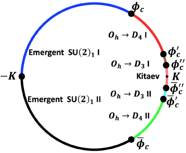
Figure 1: Phase diagram of the spin-1/2 Kitaev-Gamma chain, in which $K=\cos(\phi)$ and $\Gamma=\sin(\phi)$. The phases marked with “I” and “II” are related by the equivalence $(K,\Gamma)\cong(K,-\Gamma)$.

II Model Hamiltonian and symmetries

In this section, we first present the model Hamiltonian, and then briefly review the six-sublattice rotation and the symmetries of the system.

II.1 Model Hamiltonian

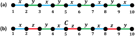
Figure 2: Bond structures in (a) the unrotated and (b) the six-sublattice rotated frames.

The Hamiltonian of the spin-1/2 Kitaev-Gamma chain is defined as Yang2019

$$H=\sum_{<ij>\in\gamma\,\text{bond}}\big{[}KS_{i}^{\gamma}S_{j}^{\gamma}+\Gamma(S_{i}^{\alpha}S_{j}^{\beta}+S_{i}^{\beta}S_{j}^{\alpha})\big{]},$$ (1)

in which $i,j$ are two sites of nearest neighbors; $\gamma=x,y$ is the spin direction associated with the $\gamma$ bond shown in Fig. 2 (a); $\alpha\neq\beta$ are the two remaining spin directions other than $\gamma$; $K$ and $\Gamma$ are the Kitaev and Gamma couplings, respectively. In what follows, the two couplings will be parametrized as

$$K=\cos(\phi),\leavevmode\nobreak\ \Gamma=\sin(\phi),$$ (2)

where $\phi\in[0,2\pi]$. Under a global spin rotation around the $z$-axis by $\pi$, i.e., $R(\hat{z},\pi):(S_{i}^{x},S_{i}^{y},S_{i}^{z})\rightarrow(S_{i}^{y},-S_{i}^{x},S_{i}^{z})$, the Kitaev term remains the same whereas $\Gamma$ changes to $-\Gamma$. Therefore, there is the equivalence

$$(K,-\Gamma)\cong(K,\Gamma),$$ (3)

or $\phi\cong 2\pi-\phi$. Due to this equivalence, the phase diagram can be restricted to the parameter range $\phi\in(0,\pi)$, and in subsequent discussions, we will drop the numbering “I” in the names of the phases for simplicity.

II.2 The six-sublattice rotation

A useful transformation $U_{6}$ with a periodicity of six sites is defined as Stavropoulos2018 ; Yang2019

$$\text{Sublattice $1$}: (x,y,z) \rightarrow(x^{\prime},y^{\prime},z^{\prime}),$$

$$\text{Sublattice $2$}: (x,y,z) \rightarrow(-x^{\prime},-z^{\prime},-y^{\prime}),$$

$$\text{Sublattice $3$}: (x,y,z) \rightarrow(y^{\prime},z^{\prime},x^{\prime}),$$

$$\text{Sublattice $4$}: (x,y,z) \rightarrow(-y^{\prime},-x^{\prime},-z^{\prime}),$$

$$\text{Sublattice $5$}: (x,y,z) \rightarrow(z^{\prime},x^{\prime},y^{\prime}),$$

$$\text{Sublattice $6$}: (x,y,z) \rightarrow(-z^{\prime},-y^{\prime},-x^{\prime}),$$ (4)

in which ”Sublattice $i$” ($1\leq i\leq 6$) denotes the sites $i+6n$ ($n\in\mathbb{Z}$), and $S^{\alpha}$ ($S^{\prime\alpha}$) is abbreviated as $\alpha$ ($\alpha^{\prime}$) for short ($\alpha=x,y,z$). After the six-sublattice rotation, the Hamiltonian $H^{\prime}=U_{6}HU_{6}^{-1}$ acquires the form

$$H^{\prime} =\sum_{<ij>\in\gamma\,\text{bond}}\big{[}-KS_{i}^{\gamma}S_{j}^{\gamma}-\Gamma(S_{i}^{\alpha}S_{j}^{\alpha}+S_{i}^{\beta}S_{j}^{\beta})\big{]},$$ (5)

in which the bond $\gamma=x,z,y$ is periodic in three sites as shown in Fig. 2 (b), and the prime has been dropped in $\vec{S}_{i}^{\prime}$ for simplicity. The explicit expression of $H^{\prime}$ in Eq. (5) is given in Appendix A.

We will stick to the six-sublattice rotated frame from here on in the remaining parts of this work unless otherwise stated. The Hamiltonian is simplified in the six-sublattice rotated frame in the sense that there is no cross term $S_{i}^{\alpha}S_{i+1}^{\beta}$ where $\alpha\neq\beta$. In particular, $H^{\prime}$ becomes SU(2) symmetric when $K=\Gamma$. Due to the equivalence established in Eq. (3), the system also has hidden SU(2) symmetry at $K=-\Gamma$. In the range $\phi\in[0,\pi]$, the points $\phi=\pi/4$ and $3\pi/4$ corresponds to an ferromagnetic (FM) and AFM Heisenberg model, respectively.

II.3 The symmetry group

In this section, the symmetry group of $H^{\prime}$ will be briefly reviewed which has been discussed in detail in Ref. Yang2019, ; Yang2020, .

The Hamiltonian $H^{\prime}$ in Eq. (5) is invariant under the time reversal operation $\mathcal{T}$, the screw operation $R_{a}T_{a}$, the coupled operation $R_{I}I$, and the global spin rotations $R(\hat{\alpha},\pi)$ ($\alpha=x,y,z$), in which: $T_{a}$ and $I$ represent the spatial translation by one site and the inversion around the point $C$ in Fig. 2 (b), respectively; $R_{a}$ and $R_{I}$ are given by $R_{a}=R(\hat{n}_{a},-2\pi/3)$ and $R_{I}=R(\hat{n}_{I},\pi)$, where $R(\hat{n},\theta)$ represents a global spin rotation around the $\hat{n}$-axis by an angle $\theta$, and the rotation axes $\hat{n}_{a}$, $\hat{n}_{I}$ are given by $\hat{n}_{a}=\frac{1}{\sqrt{3}}(1,1,1)^{T}$, $\hat{n}_{I}=\frac{1}{\sqrt{2}}(1,0,-1)^{T}$. These symmetry operations generate the symmetry group $G$ of the system:

$$G=\mathopen{<}\mathcal{T},R_{a}T_{a},R_{I}I,R(\hat{x},\pi),R(\hat{y},\pi),R(\hat{z},\pi)\mathclose{>}.$$ (6)

Notice that the spatial translation by three sites $T_{3a}=(R_{a}T_{a})^{3}$ is a group element of $G$, which generates an abelian normal subgroup. It has been shown in Ref. Yang2019, that the quotient group $G/\mathopen{<}T_{3a}\mathclose{>}$ is isomorphic to $O_{h}$, where $O_{h}$ is the full octahedral group. Therefore, the group structure of $G$ can be represented as

$$G\cong O_{h}\ltimes 3\mathbb{Z},$$ (7)

where $3\mathbb{Z}$ is $\mathopen{<}T_{3a}\mathclose{>}$ for short, and $\ltimes$ is the semi-direct product.

III Phase diagram and magnetic orders

III.1 Phase diagram

Here we give a brief summary about the phase diagram. In Ref. Yang2019, , the region $\phi\in[\phi_{c},\pi]$ is shown to be a gapless phase described by an emergent SU(2)₁ WZW model, where $\phi_{c}\simeq 0.33\pi$. Also, a conventional rank-1 spin ordered phase with an $O_{h}\rightarrow D_{4}$ symmetry breaking has been identified within $\phi\in[\phi_{c}^{\prime},\phi_{c}]$ where $\phi_{c}^{\prime}\simeq 0.10\pi$. However, the phase below $\phi_{c}^{\prime}$ was not studied in Ref. Yang2019, .

In this work, we identify the region $\phi\in[\phi_{c}^{\prime\prime},\phi_{c}^{\prime}]$ to have a classical spin order, where $\phi_{c}^{\prime\prime}\simeq 0.034\pi$ as determined from iDMRG calculations discussed in Sec. VIII. The symmetry breaking pattern is $O_{h}\rightarrow D_{3}$, and the ground state degeneracy is $|O_{h}/D_{3}|=8$. The classical $O_{h}\rightarrow D_{3}$ order has been discussed in detail in Ref. Yang2020, for the spin-$S$ Kitaev-Gamma chain in the large-$S$ limit. However, in Ref. Yang2020, where $S\geq 1$, the classical order is found to locate around $\phi=\pi/4$ which is occupied by the $O_{h}\rightarrow D_{4}$ phase in the spin-$1/2$ caseYang2019 . For the spin-1/2 Kitaev-Gamma chain, the classical order appears in the vicinity of the infinitely degenerate Brzezicki2007 Kitaev point $K=0$ where quantum fluctuations are presumably strong. In addition, we will demonstrate that the system behaves like a spin-nematic order at short and intermediate length scales, and transits into the classical order only at sufficiently long distances. Finally, the region $\phi\in[0,\phi_{c}^{\prime\prime}]$ is a different phase denoted as the “Kitaev” phase in Fig. 1 whose nature remains unclear.

Here we make some comments about the DMRG and iDMRG numerics that we have performed in the calculations. In our work, the DMRG methodWhite1992 ; White1993 was used on chains with length up to $L=96$ sites and periodic boundary conditions. Even though it is known that DMRG convergence is hard for periodic boundary conditions, we checked that our results are converged using up to $m=1200$ states with a truncation error below $10^{-6}$ as in previous investigations in Ref. Yang2019, . For iDMRG, the unit cell size is chosen as $24$, and the bond dimension is $1000$. The typical truncation error is $10^{-10}$.

III.2 The classical $O_{h}\rightarrow D_{3}$ order

In the six-sublattice rotated frame, the spin orientations in the eight-fold degenerate ground states with an $O_{h}\rightarrow D_{3}$ symmetry breaking are Yang2020

$$\vec{S}_{1+3n} = (\eta_{1}a,\eta_{2}a,\eta_{3}b)^{T},$$

$$\vec{S}_{2+3n} = (\eta_{1}a,\eta_{2}b,\eta_{3}a)^{T},$$

$$\vec{S}_{3+3n} = (\eta_{1}b,\eta_{2}a,\eta_{3}a)^{T},$$ (8)

in which $\eta_{j}=\pm 1$ ($j=1,2,3$), and $a,b$ are real numbers (in principle not necessarily positive). The “center of mass” directions of the three spins within a unit cell are plotted as the eight blue circles in Fig. 3. Here we want to emphasize that although the spin orientations within the eight degenerate ground states are all translationally invariant by three sites, they exhibit different patterns in the original frame. For the two light blue circles in Fig. 3, the two corresponding ground states exhibit a Néel order in the original frame; on the other hand, the other six dark blue circles exhibit a six-site periodicity in the original frame. More explicitly, in Fig. 4, the spin orientations in the ground states corresponding to $(1,1,1)$ and $(1,-1,1)$ vertices are plotted in the original frame which have Néel and six-site periodic patterns, respectively.

For later convenience, here we discuss the invariant correlation functions for the $O_{h}\rightarrow D_{3}$ order in the six-sublattice rotated frame. In general, the ground state of a finite size system calculated in DMRG numerics may be an arbitrary linear combination of the several nearly degenerate states (becoming exactly degenerate only in the thermodynamic limit) with the coefficients depending on numerical details. Thus the numerical results may not represent the true values of the correlation functions in the thermodynamic limit. In addition, when performing the finite size scaling, such arbitrariness may lead to a random oscillation of the correlation functions by varying the system size which does not exhibit the correct finite size scaling behavior. Therefore, one needs to construct invariant correlation functions which take the same values in the ground state subspace. As an example, consider an off-diagonal correlation function $\langle S_{1}^{x}S_{1+3n}^{y}\rangle$. It equals $a^{2}$ for the ground state corresponding to the $(1,1,1)$ vertex in Fig. 3. On the other hand, for the state corresponding to the $(1,-1,1)$ vertex, the value is $-a^{2}$. In a finite size system, it is very plausible that the finite size ground state has components on both states at $(1,\pm 1,1)$-vertices. Then there will be a cancellation so that $\langle S_{1}^{x}S_{1+3n}^{y}\rangle$ acquires some arbitrary value. This example illustrates the importance of constructing invariant correlation functions.

In fact, for the $O_{h}\rightarrow D_{3}$ symmetry breaking, it is straightforward to see that all the diagonal correlation functions

$$\left<S_{i}^{\alpha}S_{j+3n}^{\alpha}\right>$$ (9)

are invariant correlation functions, where $\alpha=x,y,z$, and $i,j=1,2,3$.

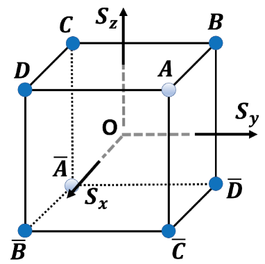
Figure 3: “Center of mass” directions of the three spins within a unit cell in the six-sublattice rotated frame as represented by the eight solid blue circles for the eight degenerate ground states in the “$O_{h}\rightarrow D_{3}$” phase. The ground states of the two solid light blue circles (along the $\pm(1,1,1)$-directions) correspond to Néel ordering in the original frame. On the other hand, the states of the six solid dark blue circles exhibit six-site periodicities in the original frame. The convention of the coordinates is taken such that the eight vertices of the cube are located at $(\pm 1,\pm 1,\pm 1)$.

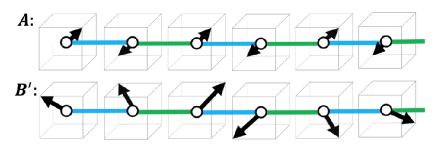
Figure 4: Spin orientations in the original frame for two representative states in Fig. 3 corresponding to the $(1,1,1)$ and $(1,-1,1)$ vertices, respectively. Pattern $A$ is Néel, and pattern $B^{\prime}$ has a six-site periodicity.

III.3 The spin-nematic order

We emphasize that the true magnetic order in the region $\phi\in[\phi_{c}^{\prime},\phi_{c}]$ is the classical $O_{h}\rightarrow D_{3}$ order. However, at short and intermediate distances, the system behaves as having a spin-nematic order with the symmetry breaking pattern $O_{h}\rightarrow D_{3d}$. Since $|O_{h}/D_{3d}|=4$, the degeneracy is four.

The spin-nematic order parameters can be determined from the $O_{h}\rightarrow D_{3d}$ symmetry breaking pattern. It turns out that there are four independent spin-nematic order parameters. In one of the four degenerate ground states, they are

$$c = \langle\Omega_{e}|S_{1}^{x}S_{2}^{z}|\Omega_{e}\rangle=\langle\Omega_{e}|S_{1}^{y}S_{2}^{x}|\Omega_{e}\rangle=\langle\Omega_{e}|S_{2}^{x}S_{3}^{z}|\Omega_{e}\rangle$$

$$= \langle\Omega_{e}|S_{2}^{z}S_{3}^{y}|\Omega_{e}\rangle=\langle\Omega_{e}|S_{3}^{y}S_{4}^{x}|\Omega_{e}\rangle=\langle\Omega_{e}|S_{3}^{z}S_{4}^{y}|\Omega_{e}\rangle,$$

$$d = \langle\Omega_{e}|S_{1}^{x}S_{2}^{y}|\Omega_{e}\rangle=\langle\Omega_{e}|S_{1}^{z}S_{2}^{x}|\Omega_{e}\rangle=\langle\Omega_{e}|S_{2}^{y}S_{3}^{z}|\Omega_{e}\rangle$$

$$= \langle\Omega_{e}|S_{2}^{z}S_{3}^{x}|\Omega_{e}\rangle=\langle\Omega_{e}|S_{3}^{x}S_{4}^{y}|\Omega_{e}\rangle=\langle\Omega_{e}|S_{3}^{y}S_{4}^{z}|\Omega_{e}\rangle,$$

$$e = \langle\Omega_{e}|S_{1}^{y}S_{2}^{z}|\Omega_{e}\rangle=\langle\Omega_{e}|S_{2}^{x}S_{3}^{y}|\Omega_{e}\rangle=\langle\Omega_{e}|S_{3}^{z}S_{4}^{x}|\Omega_{e}\rangle,$$

$$f = \langle\Omega_{e}|S_{1}^{z}S_{2}^{y}|\Omega_{e}\rangle=\langle\Omega_{e}|S_{2}^{y}S_{3}^{x}|\Omega_{e}\rangle=\langle\Omega_{e}|S_{3}^{x}S_{4}^{z}|\Omega_{e}\rangle.$$

Detailed derivations of Eq. (LABEL:eq:quadrupole_order_f) are included in Appendix B.

The other three ground states can be obtained from $|\Omega_{\alpha}\rangle=R(\hat{\alpha},\pi)|\Omega_{e}\rangle$ ($\alpha=x,y,z$), since $R(\hat{\alpha},\pi)$ are representative operations in the equivalent classes in $O_{h}/D_{3d}$. As an example, the expectation values of $e$ in the states $|\Omega_{\alpha}\rangle$ ($\alpha=x,y,z$) are given by

$$e = \langle\Omega_{x}|S_{1}^{y}S_{2}^{z}|\Omega_{x}\rangle=-\langle\Omega_{x}|S_{3}^{z}S_{4}^{x}|\Omega_{x}\rangle=-\langle\Omega_{x}|S_{2}^{x}S_{3}^{y}|\Omega_{x}\rangle,$$

$$= -\langle\Omega_{y}|S_{1}^{y}S_{2}^{z}|\Omega_{y}\rangle=\langle\Omega_{y}|S_{3}^{z}S_{4}^{x}|\Omega_{y}\rangle=-\langle\Omega_{y}|S_{2}^{x}S_{3}^{y}|\Omega_{y}\rangle,$$

$$= -\langle\Omega_{z}|S_{1}^{y}S_{2}^{z}|\Omega_{z}\rangle=-\langle\Omega_{z}|S_{3}^{z}S_{4}^{x}|\Omega_{z}\rangle=\langle\Omega_{z}|S_{2}^{x}S_{3}^{y}|\Omega_{z}\rangle.$$

III.4 The $O_{h}\rightarrow D_{4}$ order

In this subsection, we briefly summarize the $O_{h}\rightarrow D_{4}$ phase in Fig. 1 which has been analyzed in Ref. Yang2019, .

In the six-sublattice rotated frame, the spin orientations in the six-fold degenerate ground states are Yang2019

$$\vec{S}_{1+3n}=\eta b^{\prime}\hat{\alpha},\leavevmode\nobreak\ \vec{S}_{2+3n}=\eta a^{\prime}\hat{\alpha},\leavevmode\nobreak\ \vec{S}_{3+3n}=\eta a^{\prime}\hat{\alpha},$$ (12)

in which $\eta=\pm 1$, and $\alpha=x,y,z$. In the original frame, they exhibit six-site periodicities. For example, the spin orientations for the state of $\alpha=z$ in the original frame are

$$\vec{S}_{1+6n}=\hat{z},\leavevmode\nobreak\ \vec{S}_{2+6n}=-\hat{y},\leavevmode\nobreak\ \vec{S}_{3+6n}=\hat{y},$$

$$\vec{S}_{4+6n}=-\hat{z},\leavevmode\nobreak\ \vec{S}_{5+6n}=\hat{x},\leavevmode\nobreak\ \vec{S}_{6+6n}=-\hat{x}.$$ (13)

A plot of Eq. (13) is shown in Fig. 5.

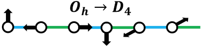
Figure 5: Spin orientations in the original frame for the $O_{h}\rightarrow D_{4}$ order.

We also discuss the invariant correlation functions for the $O_{h}\rightarrow D_{4}$ order in the six-sublattice rotated frame, which are needed in DMRG calculations. There are in total ten invariant correlation functions (for detailed discussions, see Appendix C). For our purposes, we only need the following two:

$$a^{\prime 2} = \langle S^{x}_{1}S^{x}_{2+3n}+S^{y}_{1}S^{y}_{3+3n}+S^{z}_{2}S^{z}_{3+3n}\rangle,$$

$$0 = \langle S_{1}^{y}S_{1+3n}^{z}+S_{1}^{x}S_{3+3n}^{z}+S_{2}^{x}S_{3+3n}^{y}\rangle,$$ (14)

in which $\langle...\rangle$ denotes the expectation value. In particular, since the average takes the same value within the ground state subspace, we do not need to specify which ground state the expectation value is taken in Eq. (14).

IV Misleading spin-nematic order at short and intermediate length scales

In this section, we show that at short and intermediate length scales, the system behaves as having a spin-nematic order. In particular, the time reversal symmetry remains preserved. In later sections, we will demonstrate that the time reversal symmetry is further broken at long distances, and the system transits into the classical $O_{h}\rightarrow D_{3}$ order. Therefore, there is a two-step symmetry breaking $O_{h}\rightarrow D_{3d}\rightarrow D_{3}$ as the length scale is increased.

IV.1 Ground state degeneracy

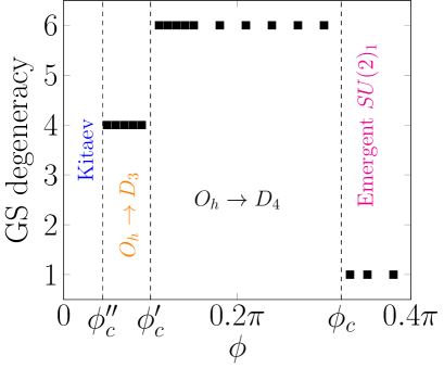
Figure 6: Ground state degeneracy as a function of $\phi$. The three phase transition points are $\phi_{c}\simeq 0.33\pi$, $\phi_{c}^{\prime}\simeq 0.10\pi$, $\phi_{c}^{\prime\prime}\simeq 0.05\pi$. ED numerics are performed on a system of $L=24$ sites with periodic boundary conditions.

	$\phi=0.06\pi$	$\phi=0.07\pi$	$\phi=0.08\pi$
$E_{1}$	-3.822078	-3.821406	-3.822237
$E_{2}-E_{1}$	$7.2\cdot 10^{-5}$	$1.0\cdot 10^{-4}$	$1.7\cdot 10^{-4}$
$E_{3}-E_{1}$	$7.2\cdot 10^{-5}$	$1.0\cdot 10^{-4}$	$1.7\cdot 10^{-4}$
$E_{4}-E_{1}$	$7.2\cdot 10^{-5}$	$1.0\cdot 10^{-4}$	$1.7\cdot 10^{-4}$
$E_{5}-E_{1}$	$7.7\cdot 10^{-4}$	$1.27\cdot 10^{-3}$	$1.84\cdot 10^{-3}$
$E_{6}-E_{1}$	$7.7\cdot 10^{-4}$	$1.27\cdot 10^{-3}$	$1.84\cdot 10^{-3}$
$E_{7}-E_{1}$	$8.6\cdot 10^{-4}$	$1.51\cdot 10^{-3}$	$2.09\cdot 10^{-3}$

	$\phi=0.09\pi$	$\phi=0.10\pi$
$E_{1}$	-3.825134	-3.830593
$E_{2}-E_{1}$	$3.35\cdot 10^{-4}$	$6.32\cdot 10^{-4}$
$E_{3}-E_{1}$	$3.35\cdot 10^{-4}$	$6.32\cdot 10^{-4}$
$E_{4}-E_{1}$	$3.35\cdot 10^{-4}$	$6.32\cdot 10^{-4}$
$E_{5}-E_{1}$	$2.28\cdot 10^{-3}$	$2.044\cdot 10^{-3}$
$E_{6}-E_{1}$	$2.28\cdot 10^{-3}$	$2.044\cdot 10^{-3}$
$E_{7}-E_{1}$	$2.33\cdot 10^{-3}$	$2.044\cdot 10^{-3}$

Table 1: Energies of several lowest lying states computed with Lanczos Exact Diagonalization. The data refer to $L=24$ sites. The four energies enclosed by the red squares are approximately degenerate at the corresponding $\phi$’s.

In Fig. 6, the ground state degeneracy is shown as a function of $\phi$. ED calculations are performed on a system of $L=24$ sites with periodic boundary conditions. Three phase transitions $\phi_{c},\phi_{c}^{\prime},\phi_{c}^{\prime\prime}$ can be identified based on the ground state degeneracy, where $\phi_{c}\simeq 0.33\pi$, $\phi_{c}^{\prime}\simeq 0.10\pi$, and $\phi_{c}^{\prime\prime}\simeq 0.05\pi$. Here we note that iDMRG gives a shifted value of $\phi_{c}^{\prime\prime}$ as will be discussed in Section VIII. When $\phi>\phi_{c}$, the ground state was nondegenerate which corresponds to the “Emergent SU(2)₁ I” phase as shown in Fig. 1. For $\phi\in[\phi_{c}^{\prime},\phi_{c}]$, the ground states are six-fold degenerate, corresponding to the $O_{h}\rightarrow D_{4}$ phase which has been identified in Ref. Yang2019, . In the range $\phi_{c}^{\prime\prime}<\phi<\phi_{c}^{\prime}$, numerics provide evidence for a four-fold ground state degeneracy, implying a spin ordering different from $O_{h}\rightarrow D_{4}$. The energies of the first seven states are displayed in Table 1, from which the four-fold ground state degeneracy can be observed. Indeed, the four energies enclosed by the red square at each angle $\phi$ are approximately degenerate, and they are separated from the other states with an energy gap much larger than the splitting among themselves. Finally, for $\phi<\phi_{c}^{\prime\prime}$, we were unable to find a definite value of the ground state degeneracy. The degeneracy has strong finite size dependences, and there is no clear energy separation between some low lying (presumably ground state) multiplet and the excited states. Therefore, no value of degeneracy is assigned to the region of $\phi<\phi_{c}^{\prime\prime}$, which is denoted as the “Kitaev” phase in Fig. 6.

Clearly, the four-fold ground state degeneracy in the region $[\phi_{c}^{\prime\prime},\phi_{c}^{\prime}]$ is not consistent with the classical $O_{h}\rightarrow D_{3}$ order which is eight-fold degenerate. In fact, in Appendix D, we are able to prove that this four-fold degeneracy is not consistent with any rank-1 magnetic order, provided that the translational symmetry $T_{3a}$ is not broken. Then the simplest possibility is the rank-2 spin-nematic order.

IV.2 Numerical evidence for spin-nematic order for $L=24$ sites

In this subsection, we provide numerical evidence for the spin-nematic order on a system of $L=24$ sites.

Define a spin-nematic-$\lambda$ field $h_{\lambda}$ as $-h_{\lambda}L\hat{Q}_{\lambda}$, where the spin-nematic operator $\hat{Q}_{\lambda}$ is the sum of the order parameters in Eq. (LABEL:eq:quadrupole_order_f), where $\lambda=c,d,e,f$. For example, $\hat{Q}_{e}$ is given by

$$\hat{Q}_{e}=\frac{1}{L}\sum_{n}(S_{1+3n}^{y}S_{2+3n}^{z}+S_{2+3n}^{x}S_{3+3n}^{y}+S_{3+3n}^{z}S_{4+3n}^{x}),$$ (15)

and the other three spin-nematic orders can be obtained similarly. Consider a small $h_{\lambda}$ field which satisfies $\Delta E\ll|e||h_{\lambda}|L\ll E_{g}$, in which $L$ is the system size, $E_{g}$ is the excitation gap, and $\Delta E$ is the finite size splitting of the ground state quartet at zero field. Suppose the system has spin-nematic orders defined in Sec. III.3, then such choice of $h_{\lambda}$ gives rise to a degenerate perturbation within the four-dimensional ground state subspace, and at the same time, no mixing between the ground states and the excited states is induced. According to Eqs. (III.3,LABEL:eq:e_xyz), the energies of the four ground states under $h_{\lambda}$ are

$$\delta E(|\Omega_{e}\rangle) = -\lambda h_{\lambda}L,$$

$$\delta E(|\Omega_{\alpha}\rangle) = \frac{1}{3}\lambda h_{\lambda}L,$$ (16)

in which $\alpha=x,y,z$, and the energy $\delta E$ is measured with respect to the zero field case. Therefore, if $\text{sgn}(h_{\lambda})=\text{sgn}(\lambda)$, $|\Omega_{e}\rangle$ is the ground state which is nondegenerate with an energy lowered by an amount $|\lambda h_{\lambda}|L$. On the other hand, if $\text{sgn}(h_{\lambda})=-\text{sgn}(\lambda)$, the ground states are three-fold degenerate, and in fact, $|\Omega_{x}\rangle,|\Omega_{y}\rangle,|\Omega_{z}\rangle$ have the same energy which is lower than the energy at zero field by an amount $\frac{1}{3}|\lambda h_{\lambda}|L$. In this way, the sign of the spin-nematic order parameter can be obtained from that of the corresponding spin-nematic field by inspecting the change of the ground state degeneracy. In addition, let $\delta E_{g}(h_{\lambda})$ be the ground state energy change with a field $h_{\lambda}$. Then according to Eq. (16), we obtain

$$\frac{\delta E_{g}(|h_{\lambda}|\text{sgn}(\lambda))}{\delta E_{g}(-|h_{\lambda}|\text{sgn}(\lambda))}=3.$$ (17)

in which $\lambda=c,d,e,f$.

(a)	$h_{c}=10^{-3}$	No field	$h_{c}=-10^{-3}$
$E_{1}$	-3.8226887	-3.8220786	-3.8222885
$E_{2}-E_{1}$	$7.99\cdot 10^{-4}$	$6.90\cdot 10^{-5}$	$3.51\cdot 10^{-5}$
$E_{3}-E_{1}$	$8.58\cdot 10^{-4}$	$6.90\cdot 10^{-5}$	$3.52\cdot 10^{-5}$
$E_{4}-E_{1}$	$8.58\cdot 10^{-4}$	$6.90\cdot 10^{-5}$	$7.68\cdot 10^{-4}$
$E_{5}-E_{1}$	$1.14\cdot 10^{-3}$	$7.68\cdot 10^{-4}$	$7.68\cdot 10^{-4}$
$E_{6}-E_{1}$	$1.14\cdot 10^{-3}$	$7.68\cdot 10^{-4}$	$8.31\cdot 10^{-4}$

(b)	$h_{d}=10^{-3}$	No field	$h_{d}=-10^{-3}$
$E_{1}$	-3.8225967	-3.8220786	-3.8222538
$E_{2}-E_{1}$	$6.945\cdot 10^{-4}$	$6.90\cdot 10^{-5}$	$3.60\cdot 10^{-5}$
$E_{3}-E_{1}$	$7.545\cdot 10^{-4}$	$6.90\cdot 10^{-5}$	$3.60\cdot 10^{-5}$
$E_{4}-E_{1}$	$7.545\cdot 10^{-4}$	$6.90\cdot 10^{-5}$	$7.75\cdot 10^{-4}$
$E_{5}-E_{1}$	$1.105\cdot 10^{-3}$	$7.68\cdot 10^{-4}$	$7.75\cdot 10^{-4}$
$E_{6}-E_{1}$	$1.105\cdot 10^{-3}$	$7.68\cdot 10^{-4}$	$8.40\cdot 10^{-4}$

(c)	$h_{e}=10^{-3}$	No field	$h_{e}=-10^{-3}$
$E_{1}$	-3.8255339	-3.8220786	-3.8234555
$E_{2}-E_{1}$	$2.339\cdot 10^{-3}$	$6.90\cdot 10^{-5}$	$7.20\cdot 10^{-6}$
$E_{3}-E_{1}$	$2.339\cdot 10^{-3}$	$6.90\cdot 10^{-5}$	$7.30\cdot 10^{-6}$
$E_{4}-E_{1}$	$2.495\cdot 10^{-3}$	$6.90\cdot 10^{-5}$	$5.60\cdot 10^{-4}$
$E_{5}-E_{1}$	$2.493\cdot 10^{-3}$	$7.68\cdot 10^{-4}$	$5.60\cdot 10^{-4}$
$E_{6}-E_{1}$	$2.537\cdot 10^{-3}$	$7.68\cdot 10^{-4}$	$7.78\cdot 10^{-4}$

(d)	$h_{f}=10^{-3}$	No field	$h_{f}=-10^{-3}$
$E_{1}$	-3.8242832	-3.8220786	-3.8228937
$E_{2}-E_{1}$	$1.847\cdot 10^{-3}$	$6.90\cdot 10^{-5}$	$2.00\cdot 10^{-6}$
$E_{3}-E_{1}$	$1.847\cdot 10^{-3}$	$6.90\cdot 10^{-5}$	$2.00\cdot 10^{-6}$
$E_{4}-E_{1}$	$1.194\cdot 10^{-3}$	$6.90\cdot 10^{-5}$	$6.21\cdot 10^{-4}$
$E_{5}-E_{1}$	$1.194\cdot 10^{-3}$	$7.68\cdot 10^{-4}$	$6.21\cdot 10^{-4}$
$E_{6}-E_{1}$	$2.070\cdot 10^{-3}$	$7.68\cdot 10^{-4}$	$8.03\cdot 10^{-4}$

Table 2: Energies of several lowest lying states computed with Lanczos Exact Diagonalization. The data refer to $L=24$ sites, and $\phi=0.06\pi$.

In Table 2, the energies of the six lowest states are displayed under different spin-nematic fields $h_{\alpha}$ ($\alpha=c,d,e,f$) at $\phi=0.06\pi$. The results are obtained from ED calculations on a system of $L=24$ sites with periodic boundary conditions. As can be seen from Table 2, the four states circled by the blue lines are separated from the other two states by an energy $\simeq 6.9\times 10^{-4}$, which is one order of magnitude larger than the energy splitting among the four states which is $\simeq 0.77\times 10^{-4}$. This provides numerical evidence for the four-fold ground state degeneracy at zero field as discussed in Fig. 6. On the other hand, as shown in Table 2, the system is nondegenerate under positive spin-nematic fields for all the four $h_{\alpha}$’s where $\alpha=c,d,e,f$, but approximately three-fold degenerate when the fields are negative. According to the previous discussions, this provides numerical evidence for the spin-nematic order parameters $c,d,e,f$ to be all positive. In addition, we check if the relations in Eq. (17) for the energy changes are satisfied. According to Table 2, the ratios $r=\delta E_{g}(|h_{\lambda}|\text{sgn}(\lambda))/\delta E_{g}(-|h_{\lambda}|\text{sgn}(\lambda))$ are

$$\begin{array}[]{ccccc}\lambda&c&d&e&f\\ r&2.91&2.96&2.51&2.70.\end{array}$$ (20)

As can be seen from Eq. (20), while the ratios for $\lambda=c,d$ agree well with $3$, there are slight deviations of $r$ from $3$ for $e,f$. In fact, the values of $e,f$ are much larger than $c,d$ (see Appendix E). Hence, a $10^{-3}$ field is too large for $e$ and $f$ in the sense that the conditions $\Delta E\ll|\lambda||h_{\lambda}|L\ll E_{g}$ are spoiled when $\lambda=e,f$. In these cases, $\delta E_{g}$ also involves the contributions from many excited states, not just the ground state quartet. Because of this reason, the relation in Eq. (17) is not satisfied to an excellent level for $h_{e},h_{f}\sim 10^{-3}$. A better agreement of $r$ with $3$ can be obtained for $e,f$ by choosing a much smaller value of the field $h_{\lambda}$.

The agreements with the predictions in Eq. (17) provide strong evidence for the spin-nematic order for a system of $L=24$ sites. Notice in particular that the non-degenerate ground state under positive $h_{\lambda}$ ($\lambda=c,d,e,f$) fields imply the absence of rank-1 magnetic orders. Otherwise the ground states has to be at least two-fold degenerate, since the applied $h_{\lambda}$ fields preserves time reversal symmetry and a sign change of the rank-1 orders by applying the time reversal operation will lead to a degenerate state with the same energy.

V Emergence of a rank-1 magnetic order at long distances

In this section, we provide numerical evidence for the emergence of a rank-1 magnetic order at long distances ($L\sim 100$). The method in Sec. IV cannot be applied, since the determination of ground state degeneracy is no longer available for large system sizes, which requires the knowledge of the energies of many finite size excited states. We will turn to an alternative method named as “energy-field relation”, which only involves the calculation of the (finite size) ground state energy, thereby can be easily pushed to much larger system sizes.

Suppose $\mathcal{O}$ is an order parameter. By adding an $\mathcal{O}$-field, the Hamiltonian becomes

$$H=H_{0}-h\mathcal{O}.$$ (21)

Let $|G_{0}\rangle$ be the particular one of the ground states of $H_{0}$ which can be polarized by $\mathcal{O}$. If the system has the $\mathcal{O}$-order, then $\langle G_{0}|\mathcal{O}|G_{0}\rangle\neq 0$. For small $h$, the energy change can be obtained from first order perturbation theory, i.e.,

$$\Delta E=E(h)-E(h=0)=-h\langle G_{0}|\mathcal{O}|G_{0}\rangle,$$ (22)

which is linear in $h$. On the other hand, If the system does not have $\mathcal{O}$-order, the energy can only change by second order perturbation theory, therefore $\Delta E\propto h^{2}$. Hence, by looking at the energy-field relation to check if it is linear or quadratic, we are able to test possible order parameters.

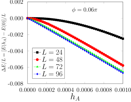
Figure 7: Energy-field relations for $h_{A}$ defined in Eq. (23) for $L=24$ (black curve), $L=48$ (red curve), $L=72$ (green curve) and $L=96$ (blue curve). Periodic boundary conditions are taken in the DMRG calculations.

Let’s consider a magnetic field $h_{A}$ along the $(1,1,1)$-direction. The Hamiltonian becomes

$$H=H^{\prime}-h_{A}\sum_{n}\frac{1}{\sqrt{3}}(S_{n}^{x}+S_{n}^{y}+S_{n}^{z}),$$ (23)

in which $H^{\prime}$ is defined in Eq. (5). The numerically calculated energy-field relation are displayed in Fig. 7 for systems of $L=24,48,72,96$ sites with periodic boundary conditions. As can be observed from Fig. 7, the energy-field relation is quadratic for $L=24$, indicating an absence of rank-1 orders consistent with the numerical results in Sec. IV. However, the energy-field relation gets increasingly more linear as the system size is increased. At $L=96$, the relation has already become very linear, implying the emergence of a rank-1 magnetic order. This shows that the spin-nematic order observed in Sec. IV is only an artifact at short and intermediate length scales.

VI Numerical evidence for the classical $O_{h}\rightarrow D_{3}$ order

In this section, we provide enough numerical evidence to show that the emerged rank-1 magnetic order at $L\sim 100$ sites in Sec. V is a classical $O_{h}\rightarrow D_{3}$ order. Throughout this section, we work in the six-sublattice rotated frame unless otherwise stated.

VI.1 Correlation functions

We first study the correlation functions both at zero fields and small magnetic fields. We fix the angle $\phi$ at $0.06\pi$, which lies within the $O_{h}\rightarrow D_{3}$ phase according to Fig. 1.

VI.1.1 Zero field

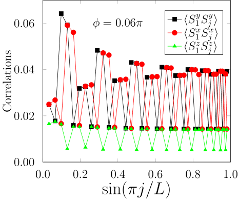
Figure 8: Correlation functions $\langle S_{1}^{x}S_{j}^{x}\rangle$ (red curve), $\langle S_{1}^{y}S_{j}^{y}\rangle$ (black) and $\langle S_{1}^{z}S_{j}^{z}\rangle$ (green) as a function of $j$. The calculations are carried out at zero field, and the system size is taken as $L=96$.

Fig. 8 plots the diagonal correlation functions $\langle S_{1}^{\alpha}S_{j}^{\alpha}\rangle$ ($\alpha=x,y,z$) as a function of $j$ calculated without magnetic field on a system of $L=96$ sites with periodic boundary conditions, where $\phi=0.06\pi$. Recall from Sec. III.2 that the diagonal correlation functions are invariant correlation functions for the $O_{h}\rightarrow D_{3}$ order. Therefore, it is legitimate to calculate $\langle S_{1}^{\alpha}S_{j}^{\alpha}\rangle$.

According to Eq. (8), at long distances, $\langle S_{1}^{\alpha}S_{j}^{\alpha}\rangle$ should be equal to

$$\langle S_{1}^{x}S_{1+3n}^{x}\rangle=a^{2},\leavevmode\nobreak\ \langle S_{1}^{x}S_{2+3n}^{x}\rangle=a^{2},\leavevmode\nobreak\ \langle S_{1}^{x}S_{3+3n}^{x}\rangle=ab,$$

$$\langle S_{1}^{y}S_{1+3n}^{y}\rangle=a^{2},\leavevmode\nobreak\ \langle S_{1}^{y}S_{2+3n}^{y}\rangle=ab,\leavevmode\nobreak\ \langle S_{1}^{y}S_{3+3n}^{y}\rangle=a^{2},$$

$$\langle S_{1}^{z}S_{1+3n}^{z}\rangle=b^{2},\leavevmode\nobreak\ \langle S_{1}^{z}S_{2+3n}^{z}\rangle=ab,\leavevmode\nobreak\ \langle S_{1}^{z}S_{3+3n}^{z}\rangle=ab.$$

As can be seen from Fig. 8, these patterns are indeed satisfied. In particular, the values of $a^{2},ab,b^{2}$ can be read as

$$a^{2}\sim 0.04,\leavevmode\nobreak\ ab\sim 0.014,\leavevmode\nobreak\ b^{2}\sim 0.005.$$ (25)

Notice that there is the relation $a^{2}\cdot b^{2}=(ab)^{2}$. Indeed, $0.04\times 0.005=2\times 10^{-4}$ is pretty close to $0.014^{2}=1.96\times 10^{-4}$. This provides evidence for the $O_{h}\rightarrow D_{3}$ order.

However, we note that the evidence is not sufficient. Denote $|\eta\hat{\alpha}\rangle$ ($\eta=\pm 1$, $\alpha=x,y,z$) as the six degenerate ground states with $O_{h}\rightarrow D_{4}$ order in which the “center of mass” direction of the three spins within a unit cell is pointing along the $\eta\hat{\alpha}$-direction as shown in Eq. (12). Then it can be easily checked that the state $\frac{1}{\sqrt{3}}(|\hat{x}\rangle+|\hat{y}\rangle+|\hat{z}\rangle)$ would produce the same patterns of correlation functions as those in Fig. 8. In the next two subsections, we test the correlation functions with small applied magnetic fields, which are able to resolve such potential concerns.

VI.1.2 Field along $(0,0,1)$-direction

Suppose we apply a small field along the $(0,0,1)$-direction, and compute the diagonal correlation functions $\left<S_{i}^{\alpha}S_{j+3n}^{\alpha}\right>$ ($\alpha=x,y,z$). If the symmetry breaking is $O_{h}\rightarrow D_{4}$, then $\left<S_{i}^{x}S_{j+3n}^{x}\right>=\left<S_{i}^{y}S_{j+3n}^{y}\right>=0$ but $\left<S_{i}^{z}S_{j+3n}^{z}\right>$ is nonzero, since the state $|\hat{z}\rangle$ is now picked out as the ground state which has an energy lower than the other five ground states at zero field. On the other hand, if the symmetry breaking is $O_{h}\rightarrow D_{3}$ order, then all of the three diagonal correlation functions are nonzero.

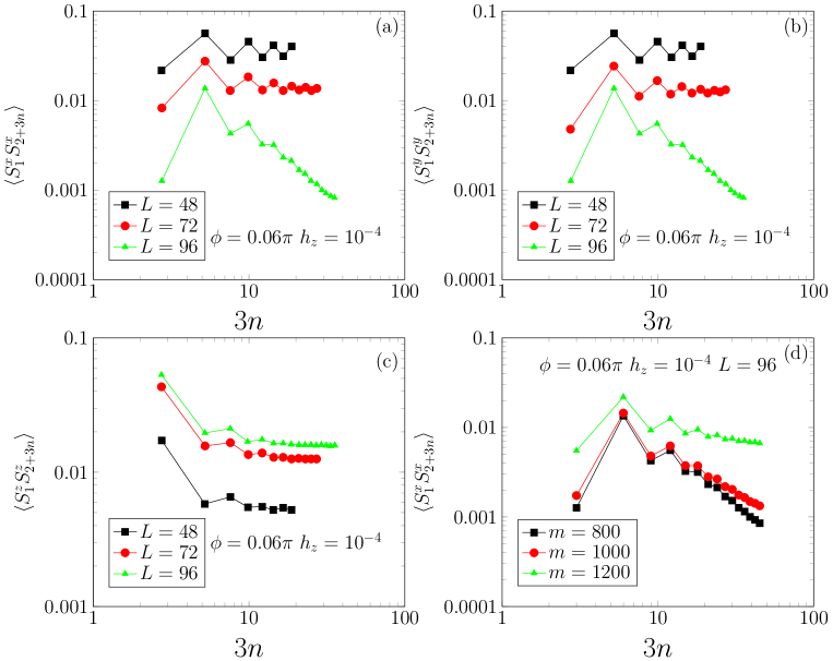
Figure 9: Diagonal correlation functions (a) $\left<S_{i}^{x}S_{j+3n}^{x}\right>$, (b) $\left<S_{i}^{y}S_{j+3n}^{y}\right>$, (c) $\left<S_{i}^{z}S_{j+3n}^{z}\right>$, and (d) $\left<S_{i}^{x}S_{j+3n}^{x}\right>$ by increasing DMRG accuracy, where a $h_{z}=10^{-4}$ field along the $(0,0,1)$-direction is applied at $\phi=0.06\pi$. DMRG numerical calculations are performed on $L=48,72,96$ sites. In (d), the number of states $m$ kept in DMRG calculations is changed from $m=800$ to $m=1200$.

Fig. 9 (a,b,c) show the DMRG numerical results for the diagonal correlation functions $\left<S_{i}^{\alpha}S_{j+3n}^{\alpha}\right>$ ($\alpha=x,y,z$) at three system sizes $L=48,72,96$. The field is chosen as $10^{-4}$ along the $(0,0,1)$-direction, and the angle is taken as $\phi=0.06\pi$. As can be seen from Fig. 9 (a,b), the $\left<S_{i}^{x}S_{j+3n}^{x}\right>$ and $\left<S_{i}^{y}S_{j+3n}^{y}\right>$ correlation functions are nonzero, indicating an $O_{h}\rightarrow D_{3}$ rather than $O_{h}\rightarrow D_{4}$ order.

However, potential concerns arise for $\left<S_{i}^{x}S_{j+3n}^{x}\right>$ and $\left<S_{i}^{y}S_{j+3n}^{y}\right>$. In fact, according to Fig. 9 (a,b), the $L=96$ results seem to exhibit a long-distance decay behavior, and it is not clear if these values go to zero at extremely long distances. To clarify this issue, we have increased the DMRG accuracy by increasing the number of states $m$ kept in DMRG calculations. The numerical results by changing $m$ are displayed in Fig. 9 (d) for $\left<S_{i}^{x}S_{j+3n}^{x}\right>$ at $L=96$. It is clear that the tail is significantly raised up when $m$ reaches $1200$. Therefore, we conclude that the decay behavior observed in Fig. 9 (a,b) at $L=96$ is possibly a numerical artifact.

VI.1.3 Field along $(1,1,1)$-direction

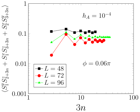
Figure 10: $O_{h}\rightarrow D_{4}$ off-diagonal correlation function $\langle S_{1}^{y}S_{2+3n}^{z}+S_{1}^{x}S_{3+3n}^{z}+S_{2}^{x}S_{3+3n}^{y}\rangle$ with a $h_{A}=10^{-4}$ field along $(1,1,1)$-direction at $\phi=0.06\pi$.

According to Eq. (14), $\langle S_{1}^{y}S_{2+3n}^{z}+S_{1}^{x}S_{3+3n}^{z}+S_{2}^{x}S_{3+3n}^{y}\rangle$ is an $O_{h}\rightarrow D_{4}$ invariant correlation function which should be zero if the symmetry breaking is $O_{h}\rightarrow D_{4}$. In Fig. 10, we apply a $h_{A}=10^{-4}$ field along the $(1,1,1)$-direction at $\phi=0.06\pi$. As can be seen from Fig. 10, the correlation function $\langle S_{1}^{y}S_{2+3n}^{z}+S_{1}^{x}S_{3+3n}^{z}+S_{2}^{x}S_{3+3n}^{y}\rangle$ is nonvanishing, which invalidates the $O_{h}\rightarrow D_{4}$ order. On the other hand, it is consistent with the $O_{h}\rightarrow D_{3}$ order, since for the ground state corresponding to the $(1,1,1)$-vertex in Fig. 3 (which is selected out by the small $(1,1,1)$-field), the off-diagonal correlation functions do not vanish.

VI.1.4 Range of the $O_{h}\rightarrow D_{3}$ phase

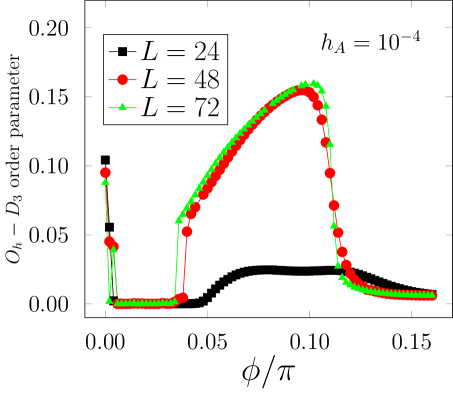
Figure 11: Off-diagonal correlation function $\langle S_{1}^{y}S_{2+3n}^{z}+S_{1}^{x}S_{3+3n}^{z}+S_{2}^{x}S_{3+3n}^{y}\rangle$ as a function of $\phi$ in the presence of a small $h_{A}=10^{-4}$ field along $(111)$-direction.

We note that the test in Sec. VI.1.3 can be efficiently used to determine the range of the $O_{h}\rightarrow D_{3}$ phase.

We have calculated the off-diagonal $O_{h}\rightarrow D_{4}$ invariant correlation function $\langle S_{1}^{y}S_{2+3n}^{z}+S_{1}^{x}S_{3+3n}^{z}+S_{2}^{x}S_{3+3n}^{y}\rangle$ in the presence of a small $h_{A}=10^{-4}$ field along the $(1,1,1)$-direction. In the $O_{h}\rightarrow D_{3}$ phase, since the ground state at the $(1,1,1)$-vertex is picked out, this correlation function is nonzero. On the other hand, in the $O_{h}\rightarrow D_{4}$ phase, it vanishes due to the off-diagonal nature.

The DMRG numerical results are shown in Fig. 11. As can be clearly seen, there is a sharp phase transition at $\phi\sim 0.035\pi$, which is $\phi_{c}^{\prime\prime}$, i.e., the transition point between the $O_{h}\rightarrow D_{3}$ and Kitaev phases. The transition at $\phi_{c}^{\prime}\sim 0.11\pi$ between $O_{h}\rightarrow D_{3}$ and $O_{h}\rightarrow D_{4}$ phases is also identifiable. Better transition values are obtained by iDMRG calculations which will be discussed in Sec. VIII.

VI.2 Spin expectation values

We further study the spin-spin correlation functions under different magnetic fields at $\phi=0.06\pi$.

VI.2.1 Field along $(1,1,1)$-direction

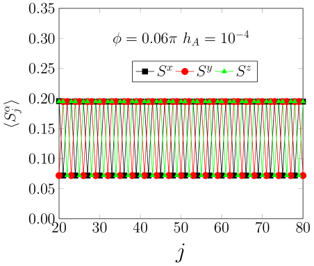
Figure 12: Spin expectation values $\left<S_{j}^{\alpha}\right>$ ($j\in\mathbb{Z},\alpha=x,y,z$) with a small $10^{-4}$ field along the $(1,1,1)$-direction. DMRG numerics are performed on $L=96$ sites at $\phi=0.06\pi$ with periodic boundary conditions.

We apply a small field $h_{A}=10^{-4}$ along the $(1,1,1)$-direction, and compute the spin expectation values $\left<S_{j}^{\alpha}\right>$ ($j\in\mathbb{Z},\alpha=x,y,z$). If the system has an $O_{h}\rightarrow D_{3}$ classical order, then the spin alignments should satisfy the following pattern,

$$\vec{S}_{1}=\left(\begin{array}[]{c}a\\ a\\ b\end{array}\right),\vec{S}_{2}=\left(\begin{array}[]{c}a\\ b\\ a\end{array}\right),\vec{S}_{3}=\left(\begin{array}[]{c}b\\ a\\ a\end{array}\right).$$ (35)

As can be seen from Fig. 12, this is indeed satisfied with $a\sim 0.20$, and $b\sim 0.075$, which is consistent with the values determined in Eq. (25).

VI.2.2 Field along $(0,0,1)$-direction

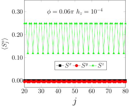
Figure 13: Spin expectation values $\left<S_{j}^{\alpha}\right>$ ($j\in\mathbb{Z},\alpha=x,y,z$) with a small $10^{-4}$ field along the $(0,0,1)$-direction. DMRG numerics are performed on $L=96$ sites at $\phi=0.06\pi$ with periodic boundary conditions.

For completeness of discussion, we also apply a small field $h_{z}=10^{-4}$ along the $(0,0,1)$-direction, and compute the spin expectation values $\left<S_{j}^{\alpha}\right>$ ($j\in\mathbb{Z},\alpha=x,y,z$). Obviously, if the system has an $O_{h}\rightarrow D_{4}$ order, then the spin alignments should satisfy the following pattern,

$$\vec{S}_{1}=\left(\begin{array}[]{c}0\\ 0\\ b^{\prime}\end{array}\right),\vec{S}_{2}=\left(\begin{array}[]{c}0\\ 0\\ a^{\prime}\end{array}\right),\vec{S}_{3}=\left(\begin{array}[]{c}0\\ 0\\ a^{\prime}\end{array}\right).$$ (45)

However, less obvious is that even if the system has an $O_{h}\rightarrow D_{3}$ order, it is still possible for the spin orientations to exhibit the pattern in Eq. (45). Consider the state

$$|G\rangle=\frac{1}{2}(|A\rangle+|B\rangle+|C\rangle+|D\rangle),$$ (46)

where $|\Lambda\rangle$ ($\Lambda=A,B,C,D$) denotes the ground state of $O_{h}\rightarrow D_{3}$ order in which the “center of mass” directions of the spins in a unit cell points to the vertex $\Lambda$ of the cube as shown in Fig. 3. Suppose the order is $O_{h}\rightarrow D_{3}$, then it can be checked in the presence of the $(0,0,1)$-field, the state $|G\rangle$ is a ground state of the system and the spin alignments are exactly given by Eq. (45).

The DMRG numerical results are displayed in Fig. 13, where $\phi=0.06\pi$ and $L=96$ with periodic boundary conditions. As can be seen from Fig. 13, Eq. (45) is satisfied. However, as discussed in above, this does not necessarily mean that the system has an $O_{h}\rightarrow D_{4}$ order.

VI.3 “Center of mass” spin directions

Previously, we have excluded the $O_{h}\rightarrow D_{4}$ order which has six degenerate ground states. However, there are still other possibilities. For example, one can imagine that the center of mass directions point to the twelve red circles in Fig. 14 (referred as 12-fold magnetic order in what follows). Therefore, we need some smoking-gun evidence for the proposed $O_{h}\rightarrow D_{3}$ order. This is what we will do in this section.

Notice that the most prominent feature of the $O_{h}\rightarrow D_{3}$ order is that the center of mass spin directions point towards the vertices of the cube. Thus, a smoking-gun study is to directly check the center of mass direction. So the strategy is to apply some small field such that the vertex $A$ in Fig. 14 is selected out, and then check whether the center of mass direction is along $(1,1,1)$.

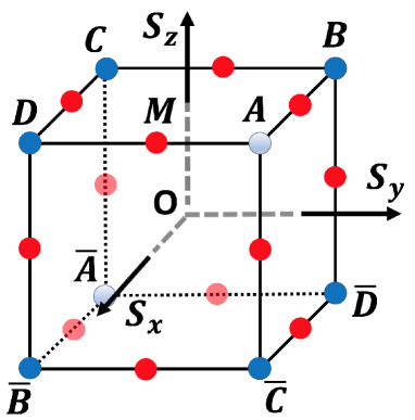
Figure 14: Center of mass spin directions for the two possible rank-1 magnetic orders with 8-fold (blue circles) and 12-fold (red circles), respectively.

The coordinates of $A,S_{z},M$ are $A=(1,1,1)$, $S_{z}=(0,0,1)$, and $M=(1,0,1)$, respectively. Let $P$ be a point lying in the triangle $AS_{z}M$. Then the advantage of a $P$-field is that it is able to select out a unique state if the system has the corresponding order. For example, if the system has $O_{h}\rightarrow D_{3}$ or $O_{h}\rightarrow D_{4}$ or 12-fold orders, then the $P$-field selects out the states located at $A$ or $S_{z}$ or $M$ correspondingly. A simple choice of $P$ would be the normalized direction of the sum of the coordinates of $A,S_{z},B$, i.e.,

$$P=\frac{1}{\sqrt{14}}(2,1,3)^{T}.$$ (47)

Define the “center of mass” spin with a unit cell as

$$\vec{S}_{c}(n)=\vec{S}_{1+3n}+\vec{S}_{2+3n}+\vec{S}_{3+3n}.$$ (48)

Define a coordinate transformation according to

$$x^{\prime} = -\frac{1}{\sqrt{6}}x+\sqrt{\frac{2}{3}}y-\frac{1}{\sqrt{6}}z,$$

$$y^{\prime} = -\frac{1}{\sqrt{2}}x+\frac{1}{\sqrt{2}}z,$$

$$z^{\prime} = \frac{1}{\sqrt{3}}x+\frac{1}{\sqrt{3}}y+\frac{1}{\sqrt{3}}z.$$ (49)

Then it is clear that the new axis $z^{\prime}$ points to the $A$ vertex. In what follows, we consider the components of $\vec{S}_{c}(n)$ in the new coordinate frame:

$$S^{x\prime}_{c}(n) = -\frac{1}{\sqrt{6}}S^{x}_{c}(n)+\sqrt{\frac{2}{3}}S^{y}_{c}(n)-\frac{1}{\sqrt{6}}S^{z}_{c}(n),$$

$$S^{y\prime}_{c}(n) = -\frac{1}{\sqrt{2}}S^{x}_{c}(n)+\frac{1}{\sqrt{2}}S^{z}_{c}(n),$$

$$S^{z\prime}_{c}(n) = \frac{1}{\sqrt{3}}S^{x}_{c}(n)+\frac{1}{\sqrt{3}}S^{y}_{c}(n)+\frac{1}{\sqrt{3}}S^{z}_{c}(n).$$ (50)

VI.3.1 “Center of mass” correlation functions

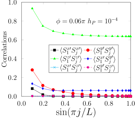
Figure 15: Correlation functions of center of mass spins in the rotated frame defined by Eq. (50) under a small $(2,1,3)$-field.

We apply a small $h_{P}$ field defined according to Eq. (47), i.e.,

$$-h_{P}\sum_{j}\frac{1}{\sqrt{14}}(2S_{j}^{x}+S_{j}^{y}+3S_{j}^{z}).$$ (51)

The field strength is taken as $h_{P}=10^{-4}$, and the system size is chosen as $L=96$ in numerical calculations. The numerical results for the correlation functions of center of mass spins are displayed in Fig. 15. If the order is $O_{h}\rightarrow D_{3}$, then only $\langle S^{z\prime}_{c}(1)S^{z\prime}_{c}(n)\rangle$ is nonzero, and all others should vanish. Indeed, as shown by Fig. 15, only $\langle S^{z\prime}_{c}(1)S^{z\prime}_{c}(n)\rangle$ is significant, and all other correlations are very small. According to our previous analysis, this provides strong evidence for the $O_{h}\rightarrow D_{3}$ order.

VI.3.2 “Center of mass” spin expectation values

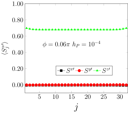
Figure 16: Expectation values of center of mass spins in the rotated frame defined by Eq. (50) under a small $(2,1,3)$-field.

This time we directly measure the spin expectation values $\langle S^{\alpha\prime}_{c}(n)\rangle$ in the new frame. If the order is $O_{h}\rightarrow D_{3}$, then only $\langle S^{z\prime}_{c}(n)\rangle$ is nonzero. As is clear from Fig. 16, indeed only $\langle S^{z\prime}_{c}(n)\rangle$ does not vanish, and both $\langle S^{x\prime}_{c}(n)\rangle$ and $\langle S^{y\prime}_{c}(n)\rangle$ are negligible.

VII Origin of classical order

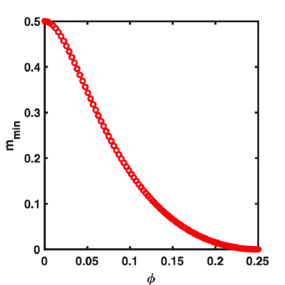
Figure 17: Smallest spin wave mass as a function of $\phi$ calculated from spin wave theory in the large-$S$ limit.

In this section, we give a naive argument for the origin of the classical order in the region where one expects strong quantum fluctuations.

As discussed in details in Ref. Yang2020, , the system has a classical $O_{h}\rightarrow D_{3}$ order for all spin values equal to or greater than $1$ in the vicinity of $\phi=0.25\pi$. So spin-$1/2$ is the only exception where the order is demonstrated to be $O_{h}\rightarrow D_{4}$. Classical analysis predicts an $O_{h}\rightarrow D_{3}$ order in the entire range $\phi\in[0,0.25\pi]$, and the eight degenerate ground states are represented by the eight blue circles in Fig. 14. When $S=1/2$, quantum fluctuations become strong, hence one would expect that the tunneling effects among these eight circles become important, which changes the potential minima from the eight vertices of the cube into the six coordinate directions $\pm\hat{\alpha}$ ($\alpha=x,y,z$), invalidating the classical analysis.

Fig. 17 displays the smallest spin wave mass $m_{\text{min}}$ calculated from the spin wave theory within the range $[0,0.25\pi]$ using the method in Ref. Yang2020, . A feature is that $m_{\text{min}}$ increases monotonically as the angle $\phi$ decreases. Naively, when $m_{\text{min}}$ is large, the potential minima become steeper, making the tunneling more difficult. Thus it is possible that in the spin-$1/2$ case, for very small $\phi$, the tunneling effects are suppressed by the larger values of the spin wave mass, and the classical order emerges. Of course, the $\phi$’s cannot be too small, otherwise the system goes into the other limit of $\phi$, which is controlled by the exactly solvable Kitaev point $\phi=0$ with an infinite ground state degeneracy Brzezicki2007 . Such intermediate $\phi$-range turns out to be $[0.033\pi,0.1\pi]$. Notice that the classical order arises from the competition between confinement of classical minima and quantum mechanical tunneling. So one would expect that the gap should be very small.

Future analytic studies about the nonclassical origin of the classical order are desired, including instanton calculations on the tunneling among classical configurations and higher order $1/S$-expansion in the framework of spin wave theory.

VIII The “Kitaev” phase

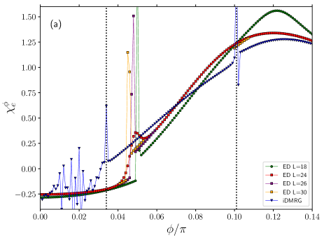
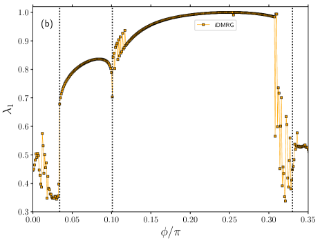
Figure 18: (a) $\chi_{e}^{\phi}$ vs $\phi$ calculated from ED for $L=18,24,26,30$ sites and iDMRG, (b) $\lambda_{1}$ vs $\phi$ calculated from iDMRG. In (a,b), the calculations are performed in the original frame defined in Eq. (1). The irregularities in the figures may come from numerical instabilities in the corresponding regions of parameters.

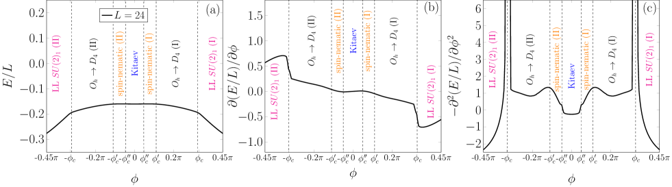
Figure 19: (a) $E/L$, (b) $\partial(E/L)/\partial\phi$, and (c) $\partial^{2}(E/L)/\partial\phi^{2}$ as functions of $\phi$. DMRG calculations are performed on $L=24$ sites with periodic boundary conditions.

In this section, we briefly discuss the “Kitaev” phase in the range $\phi\in[-\phi_{c}^{\prime\prime},\phi_{c}^{\prime\prime}]$, where the physics remains unclear. As shown in Fig. 19, the study of the ground state energy shows no signature of singularity at the AFM Kitaev point $\phi=0$, therefore the intervals $[-\phi_{c}^{\prime\prime},0]$ and $[0,\phi_{c}^{\prime\prime}]$ are likely in the same phase. As can be seen from Fig. 18 (a), the ED results of $\chi_{e}^{\phi}=-\partial^{2}e_{0}/\partial\phi^{2}$ show big peaks for $L=18,26,30$ sites around $\phi=0.05\pi$ (except $L=24$ where the peak is small), where $e_{0}=E/L$ is the ground state energy per site. However, it can be observed that the peak position shifts to smaller value of $\phi$ by increasing the system size. Indeed, the iDMRG results of $\chi_{e}^{\phi}$ in Fig. 18 (a) predicts $\phi_{c}^{\prime\prime}$ to be $0.034\pi$, which is consistent with the sudden jump of $\lambda_{1}$ in Fig. 18 (b) at the same value of $\phi$, where $\lambda_{1}$ is the largest eigenvalue of the reduced density matrix of a subsystem of $L/2-1$ sites. Based on this, we conjecture that there may be a strong finite size dependence of $\phi_{c}^{\prime\prime}$, and the thermodynamic value of $\phi_{c}^{\prime\prime}$ is possibly $0.034\pi$ as given by the iDMRG results in Fig. 18 (a,b).

The study of the ground state degeneracy in the Kitaev phase shows a strong finite size dependence and no reliable value can be extracted. In addition, we find no response to small spin-nematic nor rank-1 magnetic fields in the Kitaev phase. The AFM Kitaev point ($K>0,\Gamma=0$) is exactly solvable through Jordan-Wigner transformation, and it is known that the ground state is $2^{L-1}$-fold degenerate for a system of finite size $L$ Brzezicki2007 . In the thermodynamic limit, this becomes an exponentially large infinite degeneracy. Therefore, it is expected that there are huge quantum fluctuations in the Kitaev phase. The irregular behaviors in the Kitaev phase in the iDMRG results in Fig. 18 (a,b) possibly arise from convergence problems due to the large number of nearly degenerate states (exactly degenerate at $\phi=0$). Whether there exists a topological string order in the Kitaev phase remains to be explored further.

IX Conclusions

In summary, we have studied the phase diagram of the spin-1/2 Kitaev-Gamma chain with an AFM Kitaev coupling. In addition to the emergent SU(2)₁ and the $O_{h}\rightarrow D_{4}$ phases established in Ref. Yang2019, , two new phases are identified, i.e., a phase with $O_{h}\rightarrow D_{3}$ symmetry breaking and a “Kitaev” phase. The $O_{h}\rightarrow D_{3}$ symmetry breaking corresponds to the classical spin order, but appears in the region very close to the AFM Kitaev point where the quantum fluctuations are presumably strong. Furthermore, a two-step symmetry breaking $O_{h}\rightarrow D_{3d}\rightarrow D_{3}$ is observed as the length scale is increased. For the “Kitaev” phase, no evidence of any spin ordering nor Luttinger liquid behavior is found, and its nature remains unclear. Whether there exists any topological string order Catuneanu2019 in the “Kitaev” phase is worth further studies.

Acknowledgments WY and IA acknowledge support from NSERC Discovery Grant 04033-2016. HYK acknowledges support from NSERC Discovery Grant 06089-2016, the Centre for Quantum Materials at the University of Toronto and the Canadian Institute for Advanced Research. AN acknowledges computational resources and services provided by Compute Canada and Advanced Research Computing at the University of British Columbia. AN is supported by the Canada First Research Excellence Fund. ESS acknowledges support from NSERC Discovery Grant, SHARCNET (www.sharcnet.ca), and Compute/Calcul Canada (www.computecanada.ca).

Appendix A Explicit expressions of the Hamiltonian

In this appendix, we spell out the terms in the Hamiltonians in different frames. In general, we write the Hamiltonian $H$ as $H=\sum_{j=1}^{L}H_{j,j+1}$ where $H_{j,j+1}$ is the term on the bond between the sites $j$ and $j+1$. The forms of $H_{j,j+1}$ will be written explicitly.

In the unrotated frame, the form of $H_{j,j+1}$ has a two-site periodicity. We have

$$H_{2n+1,2n+2} = KS_{2n+1}^{x}S_{2n+2}^{x}+\Gamma(S_{2n+1}^{y}S_{2n+2}^{z}+S_{2n+1}^{z}S_{2n+2}^{y}),$$

$$H_{2n+2,2n+3} = KS_{2n+2}^{y}S_{2n+3}^{y}+\Gamma(S_{2n+2}^{z}S_{2n+3}^{x}+S_{2n+2}^{x}S_{2n+3}^{z}).$$ (52)

In the six-sublattice rotated frame, the form of $H_{j,j+1}$ has a three-site periodicity. We have

$$H^{\prime}_{3n+1,3n+2} = -KS_{3n+1}^{x}S_{3n+2}^{x}-\Gamma(S_{3n+1}^{y}S_{3n+2}^{y}+S_{3n+1}^{z}S_{3n+2}^{z}),$$

$$H^{\prime}_{3n+2,3n+3} = -KS_{3n+2}^{z}S_{3n+3}^{z}-\Gamma(S_{3n+2}^{x}S_{3n+3}^{x}+S_{3n+2}^{y}S_{3n+3}^{y}),$$

$$H^{\prime}_{3n+3,3n+4} = -KS_{3n+3}^{y}S_{3n+4}^{y}-\Gamma(S_{3n+3}^{z}S_{3n+4}^{z}+S_{3n+3}^{x}S_{3n+4}^{x}).$$ (53)

Appendix B Spin-nematic order parameters

In this appendix, we derive the spin-nematic order parameters by requiring the $O_{h}\rightarrow D_{3d}$ symmetry breaking.

Define a $9\times 9$ matrix $M$ as

$$M=\langle\Omega_{e}|\left(\begin{array}[]{c}\vec{S}_{1}\\ \vec{S}_{2}\\ \vec{S}_{3}\end{array}\right)(\vec{S}_{1}^{T}\leavevmode\nobreak\ \vec{S}_{2}^{T}\leavevmode\nobreak\ \vec{S}_{3}^{T})|\Omega_{e}\rangle,$$ (57)

in which $|\Omega_{e}\rangle$ is one of the four symmetry breaking ground states, and $\vec{S}_{i}=(S^{x}_{i},S^{y}_{i},S^{z}_{i})^{T}$ is viewed as a three-component column vector. In Eq. (57), the site indices should be understood as modulo $3$ such that the expectation values are taken for adjacent sites. For example, $S_{3}^{\alpha}S_{1}^{\beta}$ means $S_{3+3n}^{\alpha}S_{4+3n}^{\beta}$ where $n\in\mathbb{Z}$. We note that the value of $n$ is not essential in Eq. (57) since $T_{3a}$ is assumed to be unbroken. Also notice that $M$ includes all possible expectation values of adjacent-site spin-nematic order parameters.

Before proceeding on, we give the explicit expression of $D_{3d}$. Assuming the unbroken symmetry group to be

$$G_{1}=\mathopen{<}\mathcal{T},R_{a}T_{a},R_{I}I,T_{3a}\mathclose{>},$$ (58)

we will show that $G_{1}/\mathopen{<}\mathcal{T},T_{3a}\mathclose{>}$ is isomorphic to $D_{3}$. Hence, $D_{3d}$ is given by

$$D_{3d}=\mathopen{<}\mathcal{T},R_{a}T_{a},R_{I}I\mathclose{>}/\mathopen{<}T_{3a}\mathclose{>}.$$ (59)

The isomorphism $G_{1}/\mathopen{<}\mathcal{T},T_{3a}\mathclose{>}\simeq D_{3}$ can be proved using the following generator-relation representation of $D_{n}$:

$$D_{n}=\mathopen{<}a,b|a^{n}=b^{2}=(ab)^{2}=e\mathclose{>},$$ (60)

in which $e$ is the identity element. Define $a=R_{a}T_{a}$, $b=R_{I}I$. Then $a^{3}=T_{a}^{3}$, and $b^{2}=e$, which are both equal to the identity element modulo $T_{3a}$. Hence $G_{1}/\mathopen{<}T,T_{a}\mathclose{>}$ is a subgroup of $D_{3}$ since it is generated by $\{R_{a}T_{a},R_{I}I\}$. On the other hand, $\{e,R_{a},R_{a}^{-1},R_{I},R_{I}^{-1},R_{a}R_{I}\}$ are all distinct operations, and are the actions of the elements of $G_{1}/\mathopen{<}\mathcal{T},T_{a}\mathclose{>}$ restricted within the spin space. This shows that there are at least six elements in $G_{1}/\mathopen{<}\mathcal{T},T_{a}\mathclose{>}$. But the order of $D_{3}$ is six, thus $G_{1}/\mathopen{<}\mathcal{T},T_{a}\mathclose{>}$ is isomorphic to $D_{3}$.

Having $D_{3d}$ at hand, the next step is to solve the most general form of $M$ in Eq. (57) by assuming the $D_{3d}$ invariance of $|\Omega_{e}\rangle$. Since the spin-nematic order parameters automatically maintain the time reversal symmetry, $T$ has no restriction on the form of $M$ and it is enough to consider $R_{a}T_{a}$ and $R_{I}I$. Using

$$R_{a}T_{a}(\vec{S}_{1}^{T}\leavevmode\nobreak\ \vec{S}_{2}^{T}\leavevmode\nobreak\ \vec{S}_{3}^{T})(R_{a}T_{a})^{-1} = (\vec{S}_{1}^{T}\leavevmode\nobreak\ \vec{S}_{2}^{T}\leavevmode\nobreak\ \vec{S}_{3}^{T})U_{a},$$

$$R_{I}I(\vec{S}_{1}^{T}\leavevmode\nobreak\ \vec{S}_{2}^{T}\leavevmode\nobreak\ \vec{S}_{3}^{T})(R_{I}I)^{-1} = (\vec{S}_{1}^{T}\leavevmode\nobreak\ \vec{S}_{2}^{T}\leavevmode\nobreak\ \vec{S}_{3}^{T})U_{I},$$ (61)

we obtain the constraints on $M$ as

$$U_{a}MU_{a}^{-1}=M,$$ (62)

and

$$U_{I}MU_{I}^{-1}=M,$$ (63)

in which

$$U_{a}=\left(\begin{array}[]{ccc}0&0&R_{a}\\ R_{a}&0&0\\ 0&R_{a}&0\end{array}\right),\leavevmode\nobreak\ \leavevmode\nobreak\ U_{I}=\left(\begin{array}[]{ccc}0&0&R_{I}\\ 0&R_{I}&0\\ R_{I}&0&0\end{array}\right),$$ (70)

where

$$R_{a}=\left(\begin{array}[]{ccc}0&1&0\\ 0&0&1\\ 1&0&0\end{array}\right),\leavevmode\nobreak\ \leavevmode\nobreak\ R_{I}=\left(\begin{array}[]{ccc}0&0&-1\\ 0&-1&0\\ -1&0&0\end{array}\right).$$ (77)

The requirement Eq. (62) leads to

$$M=\left(\begin{array}[]{ccc}A&C^{T}&R_{a}^{-1}CR_{a}\\ C&R_{a}AR_{a}^{-1}&R_{a}C^{T}R_{a}^{-1}\\ R_{a}^{-1}C^{T}R_{a}&R_{a}CR_{a}^{-1}&R_{a}^{-1}AR_{a}\end{array}\right),$$ (81)

in which $A$ is a symmetric matrix. Eq. (62) put further constraints on $A$ and $C$ as

$$(R_{a}R_{I})A(R_{a}R_{I})^{-1} = A$$

$$(R_{a}R_{I})C(R_{a}R_{I})^{-1} = C^{T}.$$ (82)

Next we solve all possible forms of $A$ and $C$ satisfying Eq. (82). Using $R_{a}$ and $R_{I}$ given in Eq. (77), we are able to obtain

$$A=\left(\begin{array}[]{ccc}\lambda&\nu&\sigma\\ \nu&\lambda&\sigma\\ \sigma&\sigma&\mu\end{array}\right),\leavevmode\nobreak\ C=\left(\begin{array}[]{ccc}a&c&d\\ d&b&f\\ c&e&b\end{array}\right).$$ (89)

As a result, there are ten linear independent solutions of $M$, summarized as follows,

$$\lambda = \left<S_{1}^{x}S_{1}^{x}\right>=\left<S_{1}^{y}S_{1}^{y}\right>=\left<S_{2}^{x}S_{2}^{x}\right>=\left<S_{2}^{z}S_{2}^{z}\right>=\left<S_{3}^{y}S_{3}^{y}\right>=\left<S_{3}^{z}S_{3}^{z}\right>$$

$$\mu = \left<S_{1}^{z}S_{1}^{z}\right>=\left<S_{2}^{y}S_{2}^{y}\right>=\left<S_{3}^{x}S_{3}^{x}\right>$$

$$\nu = \left<S_{1}^{x}S_{1}^{y}\right>=\left<S_{1}^{y}S_{1}^{x}\right>=\left<S_{2}^{x}S_{2}^{z}\right>=\left<S_{2}^{z}S_{2}^{x}\right>=\left<S_{3}^{y}S_{3}^{z}\right>=\left<S_{3}^{z}S_{3}^{y}\right>$$

$$\sigma = \left<S_{1}^{x}S_{1}^{z}\right>=\left<S_{1}^{z}S_{1}^{x}\right>=\left<S_{1}^{y}S_{1}^{z}\right>=\left<S_{1}^{z}S_{1}^{y}\right>$$ (90)

$$= \left<S_{2}^{x}S_{2}^{y}\right>=\left<S_{2}^{y}S_{2}^{x}\right>=\left<S_{2}^{y}S_{2}^{z}\right>=\left<S_{2}^{z}S_{2}^{y}\right>$$

$$= \left<S_{3}^{x}S_{3}^{y}\right>=\left<S_{3}^{y}S_{3}^{x}\right>=\left<S_{3}^{x}S_{3}^{z}\right>=\left<S_{3}^{z}S_{3}^{x}\right>,$$

and

$$a = \left<S_{1}^{x}S_{2}^{x}\right>=\left<S_{2}^{z}S_{3}^{z}\right>=\left<S_{3}^{y}S_{4}^{y}\right>$$

$$b = \left<S_{1}^{y}S_{2}^{y}\right>=\left<S_{1}^{z}S_{2}^{z}\right>=\left<S_{2}^{x}S_{3}^{x}\right>=\left<S_{2}^{y}S_{3}^{y}\right>=\left<S_{3}^{x}S_{4}^{x}\right>=\left<S_{3}^{z}S_{4}^{z}\right>$$

$$c = \left<S_{1}^{x}S_{2}^{z}\right>=\left<S_{1}^{y}S_{2}^{x}\right>=\left<S_{2}^{x}S_{3}^{z}\right>=\left<S_{2}^{z}S_{3}^{y}\right>=\left<S_{3}^{y}S_{4}^{x}\right>=\left<S_{3}^{z}S_{4}^{y}\right>$$

$$d = \left<S_{1}^{x}S_{2}^{y}\right>=\left<S_{1}^{z}S_{2}^{x}\right>=\left<S_{2}^{y}S_{3}^{z}\right>=\left<S_{2}^{z}S_{3}^{x}\right>=\left<S_{3}^{x}S_{4}^{y}\right>=\left<S_{3}^{y}S_{4}^{z}\right>$$

$$e = \left<S_{1}^{y}S_{2}^{z}\right>=\left<S_{2}^{x}S_{3}^{y}\right>=\left<S_{3}^{z}S_{4}^{x}\right>$$

$$f = \left<S_{1}^{z}S_{2}^{y}\right>=\left<S_{2}^{y}S_{3}^{x}\right>=\left<S_{3}^{x}S_{4}^{z}\right>.$$ (91)

Among these ten solutions, the first four $\lambda,\mu,\nu,\sigma$ are on-site, which we’ll ignore. In the remaining six solutions, $a$ and $b$ are just the Kitaev and Gamma couplings which are invariant under $O_{h}$, not just $D_{3d}$, which we also ignore. Hence, the only relevant spin-nematic orders are given by $c,d,e,f$.

The spin-nematic orders $\hat{Q}_{\lambda}$ ($\lambda=c,d,e,f$) can be constructed by summing up the corresponding operators in Eq. (III.3,III.3,III.3,LABEL:eq:quadrupole_order_f). For example, $\hat{Q}_{e}$ is given by

$$\hat{Q}_{e}=\frac{1}{L}\sum_{n}(S_{1+3n}^{y}S_{2+3n}^{z}+S_{2+3n}^{x}S_{3+3n}^{y}+S_{3+3n}^{z}S_{4+3n}^{x}),$$ (92)

and the other three spin-nematic orders can be obtained similarly. There are three other degenerate ground states $|\Omega_{\alpha}\rangle$ ($\alpha=x,y,z$) which can be obtained from $|\Omega_{e}\rangle$ by

$$|\Omega_{x}\rangle = R(\hat{x},\pi)|\Omega_{e}\rangle,$$

$$|\Omega_{y}\rangle = R(\hat{y},\pi)|\Omega_{e}\rangle,$$

$$|\Omega_{z}\rangle = R(\hat{z},\pi)|\Omega_{e}\rangle,$$ (93)

where $R(\hat{\alpha},\pi)$ ($\alpha=x,y,z$) are the representative operations in the three out of four equivalent classes in $O_{h}/D_{3d}$ excluding the equivalent class containing the identity element.

It is also interesting to work out the explicit forms of the spin-nematic orders within the original frame. The spin-nematic orders in the original frame can be obtained straightforwardly by applying the inverse of the six-sublattice rotation to the expressions in Eq. (III.3,III.3,III.3,LABEL:eq:quadrupole_order_f). The spin-nematic orders thus obtained are summarized as follows,

$$\hat{Q}_{c}^{(0)} = \frac{1}{L}\sum_{j}(S_{j}^{x}S_{j+1}^{y}+S_{j}^{y}S_{j+1}^{x}),$$

$$\hat{Q}_{d}^{(0)} = \frac{1}{L}\sum_{n}(S_{1+2n}^{x}S_{2+2n}^{z}+S_{1+2n}^{z}S_{2+2n}^{x}+S_{2+2n}^{y}S_{3+2n}^{z}+S_{2+2n}^{z}S_{3+2n}^{y}),$$

$$\hat{Q}_{e}^{(0)} = \frac{1}{L}\sum_{n}(S_{1+2n}^{y}S_{2+2n}^{y}+S_{2+2n}^{x}S_{3+2n}^{x}),$$

$$\hat{Q}_{f}^{(0)} = \frac{1}{L}\sum_{j}S_{j}^{z}S_{j+1}^{z},$$ (94)

in which all the spin operators refer to the original frame.

Appendix C Invariant correlation functions in the $O_{h}\rightarrow D_{4}$ phase

In this appendix, we construct the invariant correlation functions in the $O_{h}\rightarrow D_{4}$ phase. Before proceeding to the constructions of the invariant correlation functions, we first make some comments on the symmetry breaking pattern. There are six equivalent classes in the quotient $O_{h}/D_{4}$, which is not a group since $D_{4}$ is not a normal group of $O_{h}$. The six representative elements in the equivalent classes can be chosen as the group elements in $D_{3}=\mathopen{<}R_{a}T_{a},R_{I}I\mathclose{>},\mod T_{3a}$. Notice that this is intuitively correct since $R_{a}$ and $R_{I}$ is able to rotate the $+\hat{z}$-direction to the other five directions within $\pm\hat{\alpha}$ ($\alpha=x,y,z$).

Next consider the correlation function $\langle S_{i}^{\alpha}S_{j}^{\beta}\rangle$. In what follows, we will write $i,j$ to be modulo $3$, but always bear in mind that $|i-j|\rightarrow\infty$. All the two point correlation functions are encoded in the following operators $\hat{\Phi}$,

$$\hat{\Phi}=\hat{S}^{T}\Phi\hat{S},$$ (95)

in which

$$\hat{S}=(S_{1}^{x}\leavevmode\nobreak\ S_{1}^{y}\leavevmode\nobreak\ S_{1}^{z}\leavevmode\nobreak\ S_{2}^{x}\leavevmode\nobreak\ S_{2}^{y}\leavevmode\nobreak\ S_{2}^{z}\leavevmode\nobreak\ S_{3}^{x}\leavevmode\nobreak\ S_{3}^{y}\leavevmode\nobreak\ S_{3}^{z})^{T},$$ (96)

and $\Phi$ is a $9\times 9$ numerical matrix. The $81$ independent correlation functions correspond to the $81$ choices of the matrix $\Phi$.

Let $\mathcal{U}\in D_{3}$, and $\hat{\mathcal{U}}$ be the corresponding operator in the Hilbert space. Let $U$ be a $9\times 9$ orthogonal matrix defined as

$$\hat{\mathcal{U}}^{-1}\hat{S}\hat{\mathcal{U}}=U\hat{S}.$$ (97)

Let $|\Omega_{z}\rangle$ be the ground state with all spins pointing to the $+\hat{z}$-direction. Then the other degenerate ground states can be obtained from $\hat{\mathcal{U}}|\Omega_{z}\rangle$. The invariance of the correlation function requires

$$\langle\Omega_{z}|\hat{\mathcal{U}}^{\dagger}\hat{\Phi}\hat{\mathcal{U}}|\Omega_{z}\rangle=\langle\Omega_{z}|\hat{\Phi}|\Omega_{z}\rangle.$$ (98)

Using Eq. (95) and Eq. (97), we obtain

$$\langle\Omega_{z}|\hat{S}^{T}U^{T}\Phi U\hat{S}|\Omega_{z}\rangle=\langle\Omega_{z}|\hat{S}^{T}\Phi\hat{S}|\Omega_{z}\rangle,$$ (99)

which is satisfied if

$$U^{T}\Phi U=\Phi.$$ (100)

Since $\mathcal{U}\in D_{3}$, it is enough to choose the two generators $R_{a}T_{a}$ and $R_{I}I$ of $D_{3}$. The corresponding matrix $U_{a},U_{I}$ of these two generators have already been given in Eq. (70). Therefore, we see that Eq. (100) is exactly the same as Eq. (62) for $R_{a}T_{a}$ and as Eq. (63) for $R_{I}I$. Thus the solutions of $\Phi$ are just the same as those of $M$ in Appendix B.

In summary, the ten invariant correlation functions are

$$a^{2}+2b^{2} = \vec{S}_{1}\cdot\vec{S}_{1}+\vec{S}_{2}\cdot\vec{S}_{2}+\vec{S}_{3}\cdot\vec{S}_{3},$$

$$a^{2} = S_{1}^{z}S_{1}^{z}+S_{2}^{y}S_{2}^{y}+S_{3}^{x}S_{3}^{x},$$

$$0 = (S_{1}^{x}S_{1}^{y}+S_{1}^{y}S_{1}^{x})+(S_{2}^{x}S_{2}^{z}+S_{2}^{z}S_{2}^{x})+(S_{3}^{y}S_{3}^{z}+S_{3}^{z}S_{3}^{y}),$$

$$0 = (S_{1}^{x}S_{1}^{z}+S_{1}^{z}S_{1}^{x}+S_{1}^{y}S_{1}^{z}+S_{1}^{z}S_{1}^{y})+(S_{2}^{y}S_{2}^{z}+S_{2}^{z}S_{2}^{y}+S_{2}^{x}S_{2}^{y}+S_{2}^{y}S_{2}^{x})+(S_{3}^{x}S_{3}^{z}+S_{3}^{z}S_{3}^{x}+S_{3}^{x}S_{3}^{y}+S_{3}^{y}S_{3}^{x}),$$

$$b^{2} = S^{x}_{1}S^{x}_{2}+S^{y}_{1}S^{y}_{3}+S^{z}_{2}S^{z}_{3},$$

$$2ab = (S^{y}_{1}S^{y}_{2}+S^{z}_{1}S^{z}_{2})+(S^{x}_{1}S^{x}_{3}+S^{z}_{1}S^{z}_{3})+(S^{x}_{2}S^{x}_{3}+S^{y}_{2}S^{y}_{3}),$$

$$0 = (S_{1}^{x}S_{2}^{z}+S_{1}^{y}S_{2}^{x})+(S_{1}^{x}S_{3}^{y}+S_{1}^{y}S_{3}^{z})+(S_{2}^{x}S_{3}^{z}+S_{2}^{z}S_{3}^{y}),$$

$$0 = (S_{1}^{x}S_{2}^{y}+S_{1}^{z}S_{2}^{x})+(S_{1}^{y}S_{3}^{x}+S_{1}^{z}S_{3}^{y})+(S_{2}^{y}S_{3}^{z}+S_{2}^{z}S_{3}^{x}),$$

$$0 = S_{1}^{y}S_{2}^{z}+S_{1}^{x}S_{3}^{z}+S_{2}^{x}S_{3}^{y},$$

$$0 = S_{1}^{z}S_{2}^{y}+S_{1}^{z}S_{3}^{x}+S_{2}^{y}S_{3}^{x},$$ (101)

in which the symbols $\langle\cdot\cdot\cdot\rangle$ are omitted on the right hand sides of the equations.

Appendix D Inconsistency of four-fold ground state degeneracy with rank-1 orders

In this appendix, we prove that the four-fold ground state degeneracy is not consistent with any rank-1 magnetic order. The translation symmetry by three sites is assumed to be not broken, and all symmetry operations will be considered modulo $T_{3a}$. Therefore the full symmetry group will be referred as $O_{h}$ rather than $O_{h}\ltimes 3\mathbb{Z}$.

Suppose the unbroken symmetry group to be $D$, so that the symmetry breaking pattern is $O_{h}\rightarrow D$. To obtain a four-fold degeneracy, the order of $D$ must be 12. On the other hand, the only two subgroups of $O_{h}$ that have 12 elements are the tetrahedral cubic point group $T$ and the tetragonal point group $D_{3d}$.

We show that $S_{i}^{\alpha}$ cannot be an order parameter that has either $T$ or $D_{3d}$ to be the unbroken symmetry group. Otherwise, suppose $S_{i}^{\alpha}$ acquires a nonzero expectation value on one of the four degenerate ground states $|\Omega\rangle$ which is assumed to be invariant under the cubic point group $T$. Since $R(\hat{\alpha},\pi)$ ($\alpha=x,y,z$) belongs to $T$, the sign of $S_{i}^{\alpha}$ can be changed using $R(\hat{\beta},\pi)$ where $\beta\neq\alpha$. As a result,

$$\langle\Omega|S_{i}^{\alpha}|\Omega\rangle=-\langle\Omega|R^{-1}(\beta,\pi)S_{i}^{\alpha}R(\hat{\beta},\pi)|\Omega\rangle.$$ (102)

However, since $|\Omega\rangle$ is invariant under $R(\hat{\beta},\pi)$ by assumption, we conclude that $\langle\Omega|S_{i}^{\alpha}|\Omega\rangle=-\langle\Omega|S_{i}^{\alpha}|\Omega\rangle$, which contradicts with $\langle\Omega|S_{i}^{\alpha}|\Omega\rangle\neq 0$. Thus, $T$ cannot be the unbroken symmetry group. Next we consider the possibility of $O_{h}\rightarrow D_{3d}$. In the cubic group language, $D_{3d}$ contains the inversion operation. In our case, the time reversal operation $\mathcal{T}$ plays the role of “inversion” when acting on spin operators since $T$ changes the sign of $\vec{S}_{i}$. Since the time reversal operation belongs to $D_{3d}$, it is clear that $D_{3d}$ again cannot be the unbroken symmetry group because $\vec{S}_{i}$ is odd under time reversal.

Appendix E Strength of spin-nematic orders

Figure 20: Measured spin-nematic order parameters $c$ (black) $d$ (red), $e$ (green), $f$ (blue) under small spin-nematic fields. The vertical axis is the measured value, and the results of different fields are displayed at different horizontal coordinates. All the spin-nematic fields $h_{c},h_{d},h_{e},h_{f}$ are taken positive with a magnitude equal to $10^{-3}$. In all cases, ED calculations are performed on a periodic system of $L=24$ sites at $\phi=0.06\pi$.

In this appendix, we determine the values of the spin-nematic orders $c,d,e,f$ on a system of $L=24$ sites.

We note that with a field $h_{e}$ satisfying $\text{sgn}(h_{e})=\text{sgn}(e)$, the state $|\Omega_{e}\rangle$ is selected as the ground state out of the initially four nearly degenerate ground states. Hence, we can directly compute the expectation value of the spin-nematic order parameters $S_{1+3n}^{y}S_{2+3n}^{z},S_{2+3n}^{x}S_{3+3n}^{y},S_{3+3n}^{z}S_{4+3n}^{x}$ (as given by Eq. (III.3)) in numerics. Notice that this cannot be done at zero spin-nematic fields since the true ground state in a finite size system may be an arbitrary linear combination of the four states $|\Omega_{a}\rangle$ ($a=e,x,y,z$), which leads to a random cancellation of the expectation value due to the sign differences in Eq. (III.3) and Eq. (LABEL:eq:e_xyz).

We have measured the expectation values of the spin-nematic orders under positive spin-nematic fields, and the results are shown in Fig. 20. It can be read from Fig. 20 that the expectation values are

$$c\simeq 0.014,\leavevmode\nobreak\ d\simeq 0.012,\leavevmode\nobreak\ e\simeq 0.145,\leavevmode\nobreak\ f\simeq 0.094,$$ (103)

regardless of which field $h_{\alpha}$ ($\alpha=c,d,e,f$) is applied. Here we note that as can be seen from Fig. 20, while the values of $c$ and $d$ are independent of $h_{\lambda}$ ($\lambda=c,d,e,f$), there are small variations of $e$ and $f$ under different types of spin-nematic fields. The reason is the same as before. In fact, a field of $10^{-3}$ is too large for $h_{e}$ and $h_{f}$, which mixes the ground state subspace with the excited states. As a result, in addition to the ordering in the ground state, the order paramters also acquires contributions from excited states due to a nonzero spin-nematic susceptibility. This explains why the measured values of $e$ and $f$ under $h_{e},h_{f}$ are larger than those under $h_{c},h_{d}$.

References

- (1) P. Fazekas, Lecture Notes on Electron Correlation and Magnetism, Vol. 5 of Series in Modern Condensed Matter Physics (World Scientific, 1999).
- (2) A. Läuchli, F. Mila, and K. Penc, Phys. Rev. Lett. 97, 087205 (2006).
- (3) L. Balents, Nature 464, 199 (2010).
- (4) W. Witczak-Krempa, G. Chen, Y. B. Kim, and L. Balents, Annu. Rev. Condens. Matter Phys. 5, 57 (2014).
- (5) J. G. Rau, E. K.-H. Lee, and H.-Y. Kee, Annu. Rev. Condens. Matter Phys. 7, 195 (2016).
- (6) L. Savary and L. Balents, Reports Prog. Phys. 80, 016502 (2017).
- (7) S. M. Winter, A. A. Tsirlin, M. Daghofer, J. van den Brink, Y. Singh, P. Gegenwart, and R. Valentí, J. Phys. Condens. Matter 29, 493002 (2017).
- (8) Y. Zhou, K. Kanoda, and T.-K. Ng, Rev. Mod. Phys. 89, 025003 (2017).
- (9) A. Kitaev, Ann. Phys. (N. Y.) 321, 2 (2006).
- (10) C. Nayak, S. H. Simon, A. Stern, M. Freedman, and S. Das Sarma, Rev. Mod. Phys. 80, 1083 (2008).
- (11) G. Jackeli and G. Khaliullin, Phys. Rev. Lett. 102, 017205 (2009).
- (12) J. Chaloupka, G. Jackeli, and G. Khaliullin, Phys. Rev. Lett. 105, 027204 (2010).
- (13) Y. Singh, and P. Gegenwart, Phys. Rev. B 82, 064412 (2010).
- (14) C. C. Price and N. B. Perkins, Phys. Rev. Lett. 109, 187201 (2012).
- (15) Y. Singh, S. Manni, J. Reuther, T. Berlijn, R. Thomale, W. Ku, S. Trebst, and P. Gegenwart, Phys. Rev. Lett. 108, 127203 (2012).
- (16) K. W. Plumb, J. P. Clancy, L. J. Sandilands, V. V. Shankar, Y. F. Hu, K. S. Burch, H.-Y. Kee, and Y.-J. Kim, Phys. Rev. B 90, 041112 (2014).
- (17) H.-S. Kim, V. S. V., A. Catuneanu, and H.-Y. Kee, Phys. Rev. B 91, 241110 (2015).
- (18) S.-H. Baek, S.-H. Do, K.-Y. Choi, Y. Kwon, A. Wolter, S. Nishimoto, J. van den Brink, and B. Büchner, Phys. Rev. Lett. 119, 037201 (2017).
- (19) I. A. Leahy, C. A. Pocs, P. E. Siegfried, D. Graf, S.-H. Do, K.-Y. Choi, B. Normand, and M. Lee, Phys. Rev. Lett. 118, 187203 (2017).
- (20) J. A. Sears, Y. Zhao, Z. Xu, J. W. Lynn, and Y.-J. Kim, Phys. Rev. B 95, 180411 (2017).
- (21) A. U. B. Wolter, L. T. Corredor, L. Janssen, K. Nenkov, S. Schönecker, S.-H. Do, K.-Y. Choi, R. Albrecht, J. Hunger, T. Doert, et al., Phys. Rev. B 96, 041405 (2017).
- (22) J. Zheng, K. Ran, T. Li, J. Wang, P. Wang, B. Liu, Z.-X. Liu, B. Normand, J. Wen, and W. Yu, Phys. Rev. Lett. 119, 227208 (2017).
- (23) Y. Kasahara, T. Ohnishi, N. Kurita, H. Tanaka, J. Nasu, Y. Motome, T. Shibauchi, and Y. Matsuda, Nature (London) 559, 227 (2018).
- (24) J. G. Rau, E. K.-H. Lee, and H.-Y. Kee, Phys. Rev. Lett. 112, 077204 (2014).
- (25) A. Catuneanu, Y. Yamaji, G. Wachtel, Y. B. Kim, and H.-Y. Kee, npj Quantum Mater. 3, 23 (2018).
- (26) M. Gohlke, G. Wachtel, Y. Yamaji, F. Pollmann, and Y. B. Kim, Phys. Rev. B 97, 075126 (2018).
- (27) K. Ran, J. Wang, W. Wang, Z.-Y. Dong, X. Ren, S. Bao, S. Li, Z. Ma, Y. Gan, Y. Zhang, J. T. Park, G. Deng, S. Danilkin, S.-L. Yu, J.-X. Li, and J. Wen, Phys. Rev. Lett. 118, 107203 (2017).
- (28) W. Wang, Z.-Y. Dong, S.-L. Yu, and J.-X. Li, Phys. Rev. B 96, 115103 (2017).
- (29) W. Yang, A. Nocera, T. Tummuru, H.-Y. Kee, and I. Affleck, Phys. Rev. Lett. 124, 147205 (2020).
- (30) C. E. Agrapidis, J. van den Brink, and S. Nishimoto, Sci. Rep. 8, 1815 (2018).
- (31) Wang Yang, Alberto Nocera, and Ian Affleck, Phys. Rev. Research 2, 033268 (2020).
- (32) Qiang Luo, Jize Zhao, Xiaoqun Wang, Hae-Young Kee, arXiv:2012.03382 (2020).
- (33) Zi-An Liu, Tian-Cheng Yi, Jin-Hua Sun, Yu-Li Dong, and Wen-Long You, Phys. Rev. E 102, 032127 (2020).
- (34) J. H. Gruenewald, J. Kim, H. S. Kim, J. M. Johnson, J. Hwang, M. Souri, J. Terzic, S. H. Chang, A. Said, J. W. Brill, et al., Adv. Mater. 29, 1603798 (2017).
- (35) C. E. Agrapidis, J. van den Brink, and S. Nishimoto, Phys. Rev. B 99, 224418 (2019).
- (36) A. Catuneanu, E. S. Sørensen, and H.-Y. Kee, Phys. Rev. B 99, 195112 (2019).
- (37) Erik S. Sørensen, Andrei Catuneanu, Jacob Gordon, Hae-Young Kee, Phys. Rev. X 11, 011013 (2021).
- (38) P. P. Stavropoulos, A. Catuneanu, and H.-Y. Kee, Phys. Rev. B 98, 104401 (2018).
- (39) Wang Yang, Alberto Nocera, and Ian Affleck, Phys. Rev. B 102, 134419 (2020).
- (40) W. Brzezicki, J. Dziarmaga, and A. M. Oles, Phys. Rev. B 75, 134415 (2007).
- (41) S. R. White, Phys. Rev. Lett. 69, 2863 (1992).
- (42) S. R. White, Phys. Rev. B 48, 10345 (1993).