Object classification from randomized EEG trials

Abstract

New results suggest strong limits to the feasibility of classifying human brain activity evoked from image stimuli, as measured through EEG. Considerable prior work suffers from a confound between the stimulus class and the time since the start of the experiment. A prior attempt to avoid this confound using randomized trials was unable to achieve results above chance in a statistically significant fashion when the data sets were of the same size as the original experiments. Here, we again attempt to replicate these experiments with randomized trials on a far larger (20$\times$) dataset of 1,000 stimulus presentations of each of forty classes, all from a single subject. To our knowledge, this is the largest such EEG data collection effort from a single subject and is at the bounds of feasibility. We obtain classification accuracy that is marginally above chance and above chance in a statistically significant fashion, and further assess how accuracy depends on the classifier used, the amount of training data used, and the number of classes. Reaching the limits of data collection without substantial improvement in classification accuracy suggests limits to the feasibility of this enterprise.

1 Introduction

There has been considerable recent interest in applying deep learning to electroencephalography (EEG). Two recent survey papers [4, 19] collectively contain 372 references. Much of this work attempts to classify human brain activity evoked from visual stimuli. A recent CVPR oral [21] claims to decode one of forty object classes when subjects view images from ImageNet [6] with 82.9% accuracy. Considerable follow-on work uses the same dataset [17, 14, 18, 16, 8, 2, 12, 13, 24, 7, 25, 15, 9, 11]. Our recent paper [1] demonstrates that this classification accuracy is severely overinflated due to flawed experiment design. All stimuli of the same class were presented to subjects as a single block (Fig. 1a). Further, training and test samples were taken from the same block. Because all EEG data contain long-term temporal correlations that are unrelated to stimulus processing and their design confounded block-effects with class label, Spampinato et al.[21] were classifying these long-term temporal patterns, not the stimulus class. Because the training and test samples were taken in close temporal proximity from the same block, the temporal correlations in the EEG introduced label leakage between the training and test data sets. When the experiment of Spampinato et al.[21] is repeated with randomized trials, where stimuli of different classes are randomly intermixed, classification accuracy drops to chance [1].

Another recent paper [5] attempts to remedy the shortcomings of a block design by recording two different sessions for the same subject, each organized as a block design, one to be used as training data and one to be used as test data. However, both sessions used the same stimulus presentation order (Fig. 1b). Our recent paper [1] demonstrates that classification accuracy can even be severely inflated with such a cross-session design that employs the same stimulus presentation order in both sessions due to the same long-term transients that are unrelated to stimulus processing. While an analysis of training and test sets coming from different sessions with the same stimulus presentation order yields lower accuracy than an analysis where they come from the same session, accuracy drops to chance when the two sessions have different stimulus presentation order.

All this prior work is fundamentally flawed due to improper experiment design. Essentially, the EEG signal encodes a clock and any experiment design where stimulus class correlates with time since beginning of experiment allows classifying the clock instead of the stimuli. This means that all data collected in this fashion is irreparably contaminated.

(a)
(b)
(c)

Figure 1: Stimulus presentation order and training/test splits employed by (a) Spampinato et al.[21], (b) Cudlenco et al.[5], and (c) randomized trials. (a) and (b) confound stimulus class with time since beginning of experiment.

We previously [1] attempted to replicate the experiment of Spampinato et al. [21] six times with nine different classifiers, including the LSTM employed by them, with randomized trials (Fig. 1c) instead of a block design. All attempts failed, yielding chance performance.

Here, we ask the following four questions:

1. Is it possible to decode object class from EEG data recorded from subjects viewing image stimuli with randomized stimulus presentation order?

2. If so, how many distinct classes can one decode?

3. If so, how much training data is needed?

4. If so, what classification architectures allow such decoding?

To answer these questions, we collected EEG recordings from 40,000 stimulus presentations to a single subject. To our knowledge, this is by far the largest recording effort of its kind. Moreover, we argue that collecting such a large corpus is at the bounds of feasibility; it is infeasible to collect any appreciably larger corpus. With this corpus we achieve modest ability to decode stimulus class with accuracy above chance in a statistically significant fashion. By using a greedy method to determine the most discriminable $n$ classes for $2\leq n\leq 40$, and determining the classification accuracy for each such set, we show that forty classes is at the limit of feasibility. Further, by repeating the experiments with successively larger fractions of the dataset, we determine that at least half of this large dataset is needed to achieve this accuracy. Finally, we show that an LSTM architecture previously reported to yield high accuracy [21] is unable to achieve classification accuracy above chance in a statistically significant fashion. The only two classifiers that we tried that achieve classification accuracy above chance in a statistically significant fashion are a support vector machine (SVM [3]) and the one-dimension convolutional neural network (1D CNN) previously reported by us [1].

2 Data Collection

Spampinato et al.[21] selected fifty ImageNet images from each of forty ImageNet synsets as stimuli. With one exception, we employed the same ImageNet synsets as classes (Table 1). Since we sought 1,000 images from each class, and one class, n03197337, digital watch, contained insufficient images at time of download, we replaced that class with n04555897, watch.

Table 1: ImageNet synsets employed as classes in our experiment.

n02106662 German shepherd	n02124075 Egyptian cat	n02281787 lycaenid	n02389026 sorrel	n02492035 capuchin
n02504458 African elephant	n02510455 giant panda	n02607072 anemone fish	n02690373 airliner	n02906734 broom
n02951358 canoe	n02992529 cellular telephone	n03063599 coffee mug	n03100240 convertible	n03180011 desktop computer
n04555897 watch	n03272010 electric guitar	n03272562 electric locomotive	n03297495 espresso maker	n03376595 folding chair
n03445777 golf ball	n03452741 grand piano	n03584829 iron	n03590841 jack-o-lantern	n03709823 mailbag
n03773504 missile	n03775071 mitten	n03792782 mountain bike	n03792972 mountain tent	n03877472 pajama
n03888257 parachute	n03982430 pool table	n04044716 radio telescope	n04069434 reflex camera	n04086273 revolver
n04120489 running shoe	n07753592 banana	n07873807 pizza	n11939491 daisy	n13054560 bolete

We downloaded all ImageNet images of each of the forty classes that were available on 28 July 2019, randomly selected 1,000 images for each class, resized them to 1920$\times$1080, preserving aspect ratio by padding them with black pixels either on the left and right or top and bottom, but not both, to center the image. All but one such image was either RGB or grayscale. One image, n02492035_15739, was in the CMYK color space so was transcoded to RGB for compatibility with our stimulus presentation software.

The 40,000 images were partitioned into 100 sets of 400 images each. Each set of 400 images contained exactly ten images of each of the forty classes. Each set of 400 images was randomly permuted. The order of the 100 sets of images was also randomly permuted.

A single adult male subject viewed all 100 sets of images while recording EEG. Recording was conducted over ten sessions. Each session nominally recorded data from ten sets of images, though some sessions contained fewer sets, some sessions contained more sets, and some sets were repeated due to experimenter error. (Runs per session: 10, 8, 10, 11, 11, 10, 10, 10, 10, 10. Run 19 was repeated after run 20 because one image was discovered to be in CYMK. Run 43 was repeated because one earlobe electrode was off.) When sets were repeated, only one error-free set was retained. Each recording session was nominally about six hours in duration. The subject typically took breaks after every three or so sets of images. As the EEG lab was being used for other experiments as well, recording was conducted over roughly a half-year period. (Session dates: 21, 28 Aug 2019, 3, 10, 16, 17 Sep 2019, 13, 14, 20, 21 Jan 2020.)

Our design is counterbalanced at the whole experiment level, the session level, and the run level. Each unit (experiment, session, or run) has the same number of stimulus presentations for each class with no duplicates. Thus at any level, the baseline performance is chance. This allows partial analyses of arbitrary combinations of individual runs or sessions with simple calculation of statistical significance.

Each set of 400 images was presented in a single EEG run lasting 20 minutes and 20 seconds. Each run started with 10 s of blanking, followed by 400 stimulus presentations, each lasting 2 s, with 1 s of blanking between adjacent stimulus presentations, followed by 10 s of blanking at the end of the run. There was no block structure within each run.

EEG data was recorded from 96 channels at 4,096 Hz with 24-bit resolution using a BioSemi ActiveTwo recorder and a BioSemi gel electrode cap. Two additional channels were used to record the signal from the earlobes for rereferencing. A trigger was recorded in the EEG data to indicate stimulus onset. Preprocessing software verifies that there are exactly 400 triggers in each recording.

The current analysis uses only the first 500 ms after stimulus onset for each stimulus presentation, even though 2 s of data were recorded. Further, the current analysis decimated the data from 4,096 Hz to 1,024 Hz. This was done to speed the analysis. The full dataset is available for potential future enhanced analysis.

Each session was recorded with a single capping with the cap remaining in place when the subject took breaks between runs. With fMRI data, the anatomical information captured can be used to align volumes within a run to compensate for subject motion, between runs to compensate for subjects exiting and reentering the scanner (co-registration), and between subjects to compensate for variations in brain anatomy (spatial normalization). In contrast, for EEG data, there are no established methods to adjust for differing brain/scalp anatomy when combining data from multiple subjects; often approximately corresponding scalp locations are treated as equivalent. For this reason, we recorded data from a single subject to eliminate the need to align across subjects. By performing capping only once per session and choosing a cap size to yield a snug fit, any within-session alignment issues are obviated. To minimize across-session misalignment, the same cap with pre-cut ear holes was used across sessions with the vertex marking on the cap (location Cz) positioned to be geodesically equidistant from the the nasion and inion in the front-back direction, and equidistant from the left and right pre-auricular points in the left-right direction. Furthermore, visual inspection was done from vantage points directly in front and at the back of the subject to check that the FPz, Fz, Cz, Pz, and Oz markings on the cap fell on the geodesic connecting the nasion and inion.

To check whether the subject consistently viewed the images presented, online trial averaging of the EEG data was performed in every session to obtain evoked responses that are phase-locked to the onset of the images. Data from two occipital channels (C31 and C32) were bandpass filtered in the 1–40 Hz range and epochs of 800 ms duration were segmented out synchronously following the onset of each image. Epochs with peak-to-trough fluctuations exceeding 100 mV were discarded and the remaining epochs were averaged together to yield an 800 ms-long evoked response. A clear and robust N1-P2 onset response pattern was discernible in the evoked response traces obtained in each of the 100 runs, consistent with the subject viewing the images as instructed. Note that all online averaging procedures (e.g., filtering) were done to data in a separate buffer; the raw unprocessed data from 96 channels was saved for offline analysis.

3 Preprocessing

The raw EEG data was recorded in bdf file format, a single file for each of the 100 runs. We performed minimal preprocessing on this data, independently for each run, first rereferencing the data to the earlobes, then extracting exactly 0.5 s of data starting at each trigger, then z-scoring each channel of the extracted samples for each run independently, so that the extracted samples for each channel of each run have zero mean and unit variance, and then finally decimating the signal from 4,096 Hz to 1,024 Hz. No filtering was performed. After rereferencing, there is no appreciable line noise to filter. Randomized trials preclude classifying long-term transients, thus there is no need to filter out such transients. Note that this preprocessing is minimal; future studies should consider improving the SNR of the neural signals by manually removing artifacts from eye blinks, movements, and facial muscle artifacts.

The data was then randomly partitioned into five equal-sized folds, each containing the same number of samples of each class. All analyses below report average across five-fold round-robin leave-one-fold-out cross validation, taking four folds in each split as training data and the remaining fold as test data. When performing analyses on subsets of the data, the sizes of the folds, and thus the sizes of the training and test sets, varied proportionally.

4 Classifiers

The analyses below employ five different classifiers, an LSTM [10], a nearest neighbor classifier ($k$-NN), an SVM, a two-layer fully-connected neural network (MLP), and a one-dimensional CNN. The LSTM is the same as Spampinato et al.[21] with the modifications discussed previously by us [1]. The remainder are as described previously by us [1], with minor differences resulting from the fact that here the signals contain 512 temporal samples instead of 440.

5 Analyses

To answer the first question, Is it possible to decode object class from EEG data recorded from subjects viewing image stimuli with randomized stimulus presentation order?, we trained and tested each of the five classifiers on the entire dataset of 1,000 stimulus presentations of each of forty classes, using five-fold cross validation (Table 2). All analyses here and below test statistical significance above chance using $p<\textrm{0.005}$ against a null hypothesis by a binomial cmf. Only two classifiers, the SVM and the 1D CNN, yield statistically significant above-chance accuracy.

Table 2: Classification accuracy on the validation set, averaged across all five folds, for each classifier. Here and throughout, starred values indicate statistical significance above chance ($p<\textrm{0.005}$) by a binomial cmf.

LSTM	$k$-NN	SVM	MLP	1D CNN
2.2%	2.1%	5.0%∗	2.5%	5.1%∗

To answer the second question, How many distinct classes can one decode?, we performed a greedy analysis, independently for each classifier. We first trained and tested a classifier for each pair of distinct classes. Figs. 2–6 depict the resulting average validation accuracies. Only one classifier, the SVM, yielded a statistically significant above-chance accuracy for some pair. It did so for a large number of pairs. We then selected the pair with the highest average validation accuracy, independently for each classifier, and selected the first element of this pair as the seed for a class sequence for that classifier. Then for each $n$ between two and forty, we greedily and incrementally added one more class to the class sequence for each classifier. This class was selected by trying each unused class, adding it to the class sequence, training and testing a classifier with that addition, and selecting the added class that led to the highest classification accuracy. This yielded a distinct class sequence of next-most-discriminable classes for each classifier, along with an average validation accuracy on each initial prefix of that sequence (Fig. 7 left and Table 3 left). With the exception of a single data point, the MLP classifier achieving marginally significant above-chance classification accuracy for $n=29$, only two classifiers, the SVM and the 1D CNN, yielded statistically significant above-chance accuracy for any number of classes. They both yielded statistically significant above-chance accuracy for all numbers of classes.

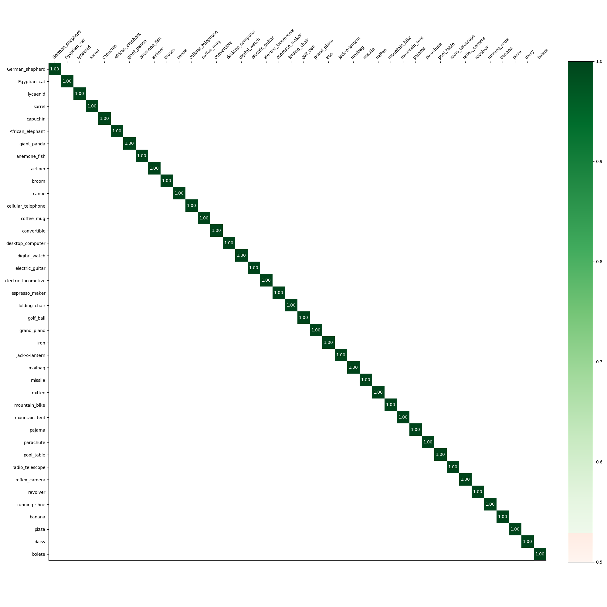
Figure 2: Two-class classification accuracy on the validation set, averaged across all five folds, for each pair of classes and the LSTM classifier. Green denotes statistical significance above chance ($p<\textrm{0.005}$) by a binomial cmf. Red denotes above chance but not statistically significant. Blank denotes at or below chance.

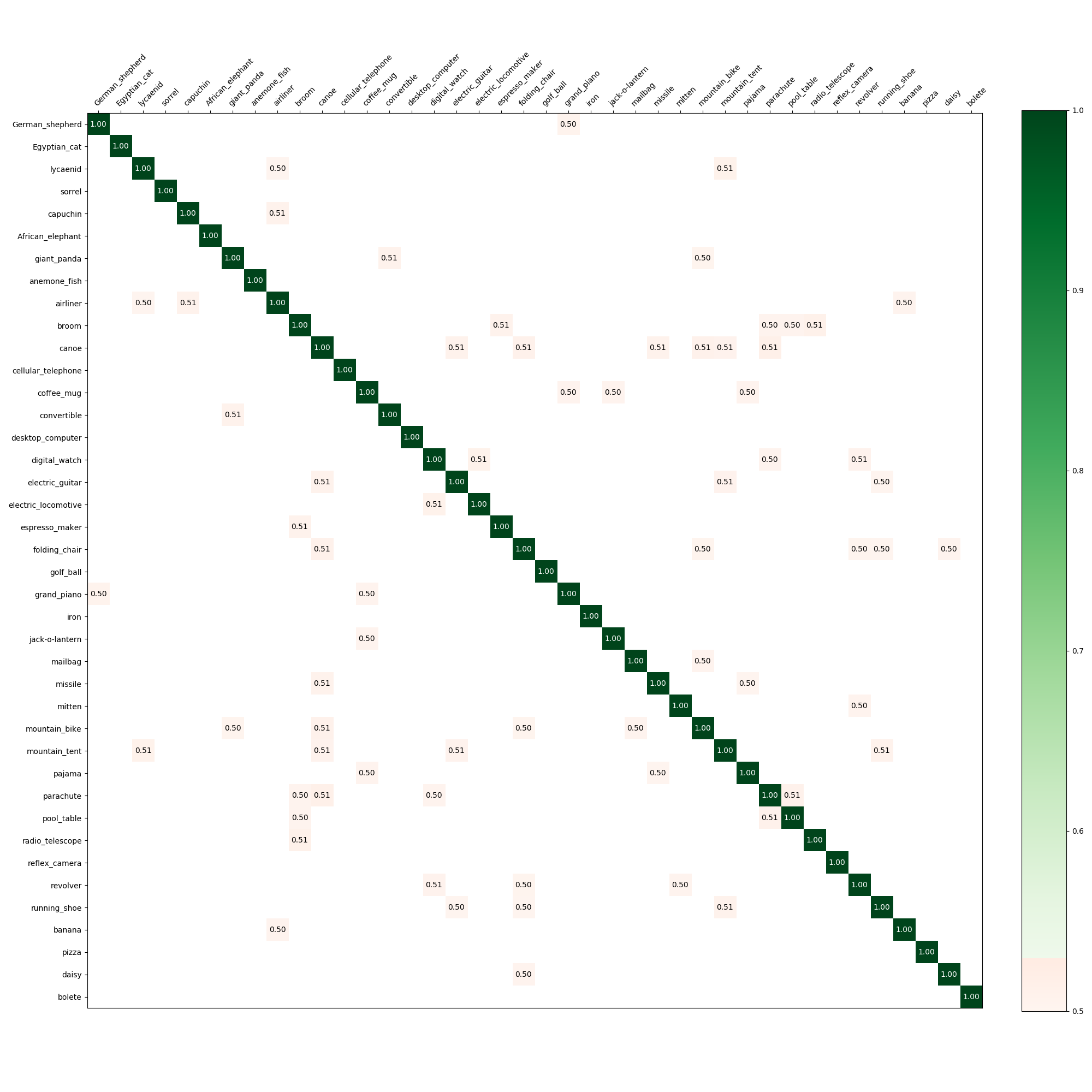
Figure 3: Variant of Fig. 2 for the $k$-NN classifier.

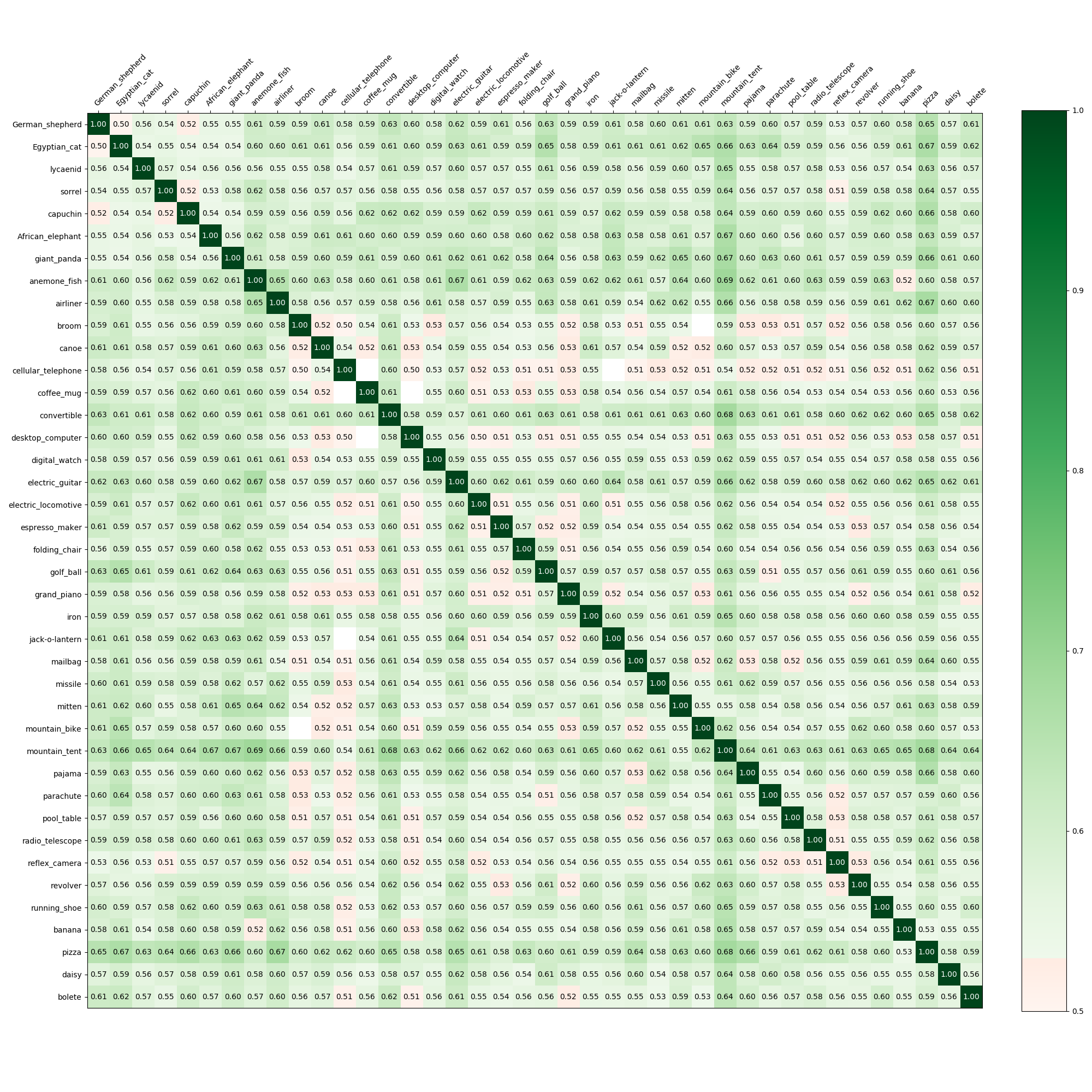
Figure 4: Variant of Fig. 2 for the SVM classifier.

Figure 5: Variant of Fig. 2 for the MLP classifier.

Figure 6: Variant of Fig. 2 for the 1D CNN classifier.

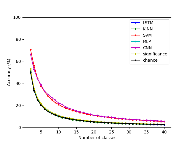
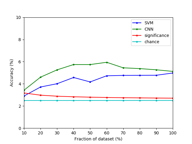
Figure 7: (left) Classification accuracy on the validation set, averaged across all five folds, as a function of the number of classes, for each classifier, for the most discriminable subset of classes as determined by the greedy algorithm. This plot contains all data points for the LSTM, SVM, MLP, and 1D CNN classifiers and 35 data points for the $k$-NN classifier. The remaining classifier runs are in progress. (They require several months on our cluster of 54 GPUs.) This plot will be replaced with a complete plot in a final version of this manuscript if accepted. (right) Classification accuracy on the validation set, for all forty classes as a function of the fraction of the dataset used for train and test, for the two classifiers for which accuracy is above chance in a statistically significant fashion. Significance denotes above chance ($p<\textrm{0.005}$) by a binomial cmf. Tabular versions of these plots are in Table 3.

Table 3: Tabular version of Fig. 7.

accuracy number of classes LSTM $k$-NN SVM MLP 1D CNN 2 50.0% 51.3% 70.8%∗ 50.0% 66.4%∗ 3 33.3% 33.8% 56.1%∗ 33.7% 52.5%∗ 4 25.5% 25.1% 44.5%∗ 26.7% 44.1%∗ 5 20.8% 20.7% 37.5%∗ 21.1% 38.4%∗ 6 17.1% 16.9% 32.4%∗ 17.4% 32.8%∗ 7 14.8% 14.4% 28.3%∗ 14.9% 29.8%∗ 8 12.7% 12.6% 25.1%∗ 13.3% 27.1%∗ 9 11.3% 10.9% 22.6%∗ 11.9% 24.7%∗ 10 10.1% 9.7% 20.6%∗ 10.5% 22.0%∗ 11 9.4% 8.7% 18.9%∗ 9.2% 20.9%∗ 12 8.4% 8.1% 17.5%∗ 8.7% 18.4%∗ 13 8.0% 7.4% 16.3%∗ 8.2% 17.2%∗ 14 7.2% 6.9% 15.2%∗ 7.5% 16.2%∗ 15 6.7% 6.4% 14.3%∗ 6.9% 14.8%∗ 16 6.2% 6.0% 13.4%∗ 6.5% 14.0%∗ 17 5.9% 5.7% 12.7%∗ 6.1% 13.6%∗ 18 5.5% 5.3% 12.0%∗ 5.8% 12.5%∗ 19 5.1% 5.0% 11.4%∗ 5.4% 11.9%∗ 20 4.8% 4.7% 10.8%∗ 5.3% 11.0%∗ 21 4.7% 4.5% 10.3%∗ 4.9% 10.9%∗ 22 4.4% 4.2% 9.8%∗ 4.8% 10.0%∗ 23 4.2% 4.1% 9.4%∗ 4.5% 9.4%∗ 24 4.0% 3.9% 9.0%∗ 4.4% 9.4%∗ 25 3.8% 3.8% 8.6%∗ 4.0% 9.1%∗ 26 3.7% 3.6% 8.3%∗ 3.9% 8.6%∗ 27 3.5% 3.5% 8.0%∗ 4.0% 8.1%∗ 28 3.5% 3.4% 7.7%∗ 3.7% 8.1%∗ 29 3.3% 3.3% 7.4%∗ 3.8%∗ 7.5%∗ 30 3.4% 3.2% 7.2%∗ 3.3% 7.3%∗ 31 3.1% 3.1% 6.9%∗ 3.4% 7.1%∗ 32 3.0% 3.0% 6.7%∗ 3.2% 7.0%∗ 33 3.0% 2.8% 6.5%∗ 3.1% 6.7%∗ 34 2.8% 2.7% 6.3%∗ 2.9% 6.4%∗ 35 2.8% 2.6% 6.1%∗ 2.8% 6.4%∗ 36 2.6% 2.5% 5.9%∗ 2.7% 6.2%∗ 37 2.6% 5.7%∗ 2.8% 6.1%∗ 38 2.5% 5.5%∗ 2.6% 5.9%∗ 39 2.4% 5.3%∗ 2.5% 5.7%∗ 40 2.3% 5.2%∗ 2.4% 5.4%∗

accuracy fraction of dataset SVM 1D CNN 10% 2.9% 3.4%∗ 20% 3.7%∗ 4.6%∗ 30% 4.0%∗ 5.3%∗ 40% 4.6%∗ 5.7%∗ 50% 4.2%∗ 5.7%∗ 60% 4.7%∗ 5.9%∗ 70% 4.8%∗ 5.4%∗ 80% 4.8%∗ 5.4%∗ 90% 4.8%∗ 5.3%∗ 100% 5.0%∗ 5.1%∗

To answer the third question, How much training data is needed?, we performed an analysis where classifiers were trained and tested on progressively larger portions of the dataset, starting with 10%, incrementing by 10%, until the full dataset was tested. This was done by taking the first ten runs and incrementally adding the next ten runs. This was done only for the SVM and the 1D CNN, as only these had statistically significant above-chance accuracy (Fig. 7 right and Table 3 right). Validation accuracy generally increases with the availability of more training data, though growth tapers off demonstrating diminishing returns.

Finally, the fourth question, What classification architectures allow such decoding?, was implicitly answered by the above three analyses. Only the SVM and the 1D CNN answer any of the above three questions in the affirmative. The SVM and the 1D CNN answer all of the above three questions in the affirmative.

6 Significance

With our data collection, each run lasted 20:20. The recording alone for each session nominally took 3:23:20. Including capping, uncapping, subject breaks, setup, teardown, and data transfer, each session took more than six hours, i.e., most of a full business day. The ten sessions required to collect our dataset took more than sixty hours, i.e., most of two full business weeks. Few subjects would consent to, and complete, such an extensive and tedious data collection effort. Consider what it would take to collect a larger dataset. Collecting EEG recordings of a single subject viewing all 1,431,167 images of ILSVRC 2012 [20] would take more than a full business year with the protocol employed in this manuscript. Doing so for all 14,197,122 images and 21,841 synsets currently included in ImageNet (3 Feb 2020) would take more than a full business decade. We doubt that any subject would consent to, and complete, such an extensive and tedious data collection effort. Moreover, we doubt that any EEG lab would dedicate the resources needed to do so.

7 Related Work

We know of two prior attempts at collecting large EEG datasets. The “MNIST” of Brain Digits recorded EEG data from a single subject viewing 186,702 presentations of the digits 0–9, each for 2 s, over a two-year period [23]. (While this dataset is called “MNIST,” it is unclear what stimuli the subject viewed.) It was recorded by the subject themselves with four different consumer-grade EEG recording devices (Neurosky Mindwave, Emotiv EPOC, Interaxon Muse, and Emotiv Insight), each with only a handful of electrodes (Mindwave: 1, EPOC: 14, Muse: 4, and Insight: 5). “IMAGENET” of The Brain recorded EEG data from a single subject viewing 14,012 stimulus presentations spanning 13,998 ILSVRC 2013 training images and 569 classes, each for 3 s, over a one-year period [22]. The number of images per class ranged from 8 to 44. Fourteen images were presented as stimuli twice. It was recorded by the subject themselves with a single consumer-grade EEG recording device (Emotiv Insight) with five electrodes. (The number of ‘brain signals’ reported by Vivancos [23, 22] differ from the above due to multiplication of the stimulus presentations by the number of electrodes.)

While we applaud such efforts, several issues arise with these datasets. Consumer grade recording devices have far fewer electrodes, far lower sample rate, and far lower resolution than research-grade EEG recording devices. They use dry electrodes instead of gel electrodes. There is no control over electrode placement. It is unclear how to use recordings from different devices with different numbers and configurations of electrodes as part of a common experiment. The designs were not counterbalanced. The stimulus presentation order is not clear so it is not clear whether these datasets suffer from the issues described previously by us [1]. The recording did not appear to employ a trigger so it is unclear how to determine the stimulus onset. The reduced precision limits the utility of these datasets. Moreover, the “MNIST” of Brain Digits has too few classes and “IMAGENET” of The Brain has too few stimuli per class to answer the questions we pose here.

A significant amount of prior work suffers irreparably from flawed EEG experiment design. The dataset collected by Spampinato et al.[21] is contaminated by its combination of block design and having all images of a class appear in only one block. Unfortunately, this fundamental design confound cannot be overcome by post processing. Considerable follow-on work [17, 14, 18, 16, 8, 2, 12, 13, 24, 7, 25, 15, 9, 11] that uses this dataset also inherits this confound and their conclusions may thus be flawed. We previously [1] demonstrated that accuracy drops to chance when such flawed designs are replaced with randomized trials keeping all other aspects of the experiment design unchanged, including the dataset size. Here we demonstrate that accuracy increases to only marginally above significance even when the dataset size is increased to the bounds of feasibility.

8 Conclusion and Summary of Novel Contributions

In this manuscript we demonstrate five novel contributions.

1. We show that it does not seem possible to decode object class from EEG data recorded from subjects viewing image stimuli with randomized stimulus presentation order when the dataset contains between two and forty classes with classification accuracy that is above chance in a statistically significant fashion using an LSTM (the classifier employed by Spampinato et al.[21]), a $k$-NN, or an MLP classifier, even if one has a training set that is 20$\times$ larger than previous work. It appears that LSTM, $k$-NN, and MLP classifiers are ill-suited to classifying object class from EEG data recorded from subjects viewing image stimuli no matter how many classes are classified and no matter how much training data is available. This refutes a large amount of prior work and shows that the task attempted by that work is simply infeasible.

2. We show that it is possible to decode object class from EEG data recorded from subjects viewing image stimuli with randomized stimulus presentation order when the dataset contains between two and forty classes with classification accuracy that is marginally above chance in a statistically significant fashion using either an SVM classifier or the 1D CNN classifier proposed previously by us [1]. However, it is not possible to obtain accuracy above chance in a statistically significant fashion with a dataset of the size employed by previous work (fifty samples per class). For forty classes, accuracy is marginally below statistical significance for the SVM and marginally above statistical significance for the 1D CNN with 100 samples per class (2$\times$ previous work) and increases to about 5% for the SVM and 6% for the 1D CNN with about 600 samples per class (12$\times$ previous work) and then tapers off. It appears that no amount of additional training data will allow substantially better classification accuracy for forty classes using the classifiers that we tried.

3. Our classification accuracies are state-of-the-art for decoding object class from EEG data recorded from subjects viewing image stimuli with randomized stimulus presentation and large numbers of classes. To our knowledge, these are also the first results yielding statistically significant above-chance accuracy with a large number of classes. Previous reports of higher accuracy, to the best of our knowledge, appear to use data that are contaminated by the confounds we describe.

4. We show that gathering the amounts of training data to achieve this level of accuracy are at the bounds of feasibility. Gathering the requisite data to train classifiers for a larger number of classes, such as all of ILSVRC 2012, let alone all of ImageNet, would require Herculean effort.

5. We collected by far the largest known dataset of EEG recordings from a single subject viewing image stimuli with professional grade equipment and procedures using proper randomized trials. It has 20$\times$ as many stimuli per class as our previous dataset [1], 4$\times$ as many classes as the dataset of Vivancos [23] (which is not known to have randomized trials), and 23$\times$ to 125$\times$ as many stimuli per class as the dataset of Vivancos [22] (which is also not known to have randomized trials). We will release this dataset upon publication. This will facilitate experimentation with new classification and analysis methods that will hopefully lead to improved accuracy in the future.

Despite recent claims to the contrary, presented to the computer-vision community with great fanfare, the problem of classifying visually perceived objects from EEG recordings with high accuracy for large numbers of classes is immensely difficult and currently beyond the state of the art. It appears to be infeasible and may even be impossible. A common euphoria in the community is that large datasets have allowed deep-learning methods to solve practically everything. It appears, however, to have reached its limit with object classification from EEG recordings. Neither heroic amounts of data, at the bounds of feasibility, nor the standard deep-learning architectures of fully connected networks (MLP), convolutional neural networks (CNN), or recurrent neural networks (LSTM)—or even more traditional machine-learning methods like nearest-neighbor classifiers ($k$-NN) or support vector machines (SVM), appear suited to the task. We present our data and this task to the community as a challenge problem for moving beyond large datasets and deep learning, to true understanding of human visual perception.

References

- [1] Anonymous Authors: The perils and pitfalls of block design for EEG classification experiments. IEEE Transactions on Pattern Analysis and Machine Intelligence (in press)
- [2] Bozal, A.: Personalized Image Classification from EEG Signals using Deep Learning. B.S. thesis, Universitat Politècnica de Catalunya (2017)
- [3] Cortes, C., Vapnik, V.: Support-vector networks. Machine Learning 20(3), 273–297 (1995)
- [4] Craik, A., He, Y., Contreras-Vidal, J.L.: Deep learning for electroencephalogram (EEG) classification tasks: a review. Journal of Neural Engineering 16(3) (2019)
- [5] Cudlencu, N., Popescu, N., Leordeanu, M.: Reading into the mind’s eye: Boosting automatic visual recognition with EEG signals. Neurocomputing available online 23 December 2019 (2019)
- [6] Deng, J., Dong, W., Socher, R., Li, L.J., Li, K., Fei-Fei, L.: Imagenet: A large-scale hierarchical image database. In: Computer Vision and Pattern Recognition. pp. 248–255 (2009)
- [7] Du, C., Du, C., He, H.: Doubly semi-supervised multimodal adversarial learning for classification, generation and retrieval. In: International Conference on Multimedia and Expo. pp. 13–18 (2019)
- [8] Du, C., Du, C., Xie, X., Zhang, C., Wang, H.: Multi-view adversarially learned inference for cross-domain joint distribution matching. In: International Conference on Knowledge Discovery & Data Mining. pp. 1348–1357 (2018)
- [9] Fares, A., Zhong, S., Jiang, J.: Region level bi-directional deep learning framework for EEG-based image classification. In: International Conference on Bioinformatics and Biomedicine. pp. 368–373 (2018)
- [10] Hochreiter, S., Schmidhuber, J.: Long short-term memory. Neural Computation 9(8), 1735–1780 (1997)
- [11] Hwang, S., Hong, K., Son, G., Byun, H.: EZSL-GAN: EEG-based zero-shot learning approach using a generative adversarial network. In: International Winter Conference on Brain-Computer Interface (2019)
- [12] Jiang, J., Fares, A., Zhong, S.H.: A context-supported deep learning framework for multimodal brain imaging classification. IEEE Transactions on Human-Machine Systems (2019)
- [13] Jiao, Z., You, H., Yang, F., Li, X., Zhang, H., Shen, D.: Decoding EEG by visual-guided deep neural networks. In: International Joint Conference on Artificial Intelligence (2019)
- [14] Kavasidis, I., Palazzo, S., Spampinato, C., Giordano, D., Shah, M.: Brain2Image: Converting brain signals into images. In: ACM Multimedia Conference. pp. 1809–1817 (2017)
- [15] Mukherjee, P., Das, A., Bhunia, A.K., Roy, P.P.: Cogni-Net: Cognitive feature learning through deep visual perception. In: International Conference on Image Processing. pp. 4539–4543 (2019)
- [16] Palazzo, S., Kavasidis, I., Kastaniotis, D., Dimitriadis, S.: Recent advances at the brain-driven computer vision workshop. In: European Conference on Computer Vision (2018)
- [17] Palazzo, S., Spampinato, C., Kavasidis, I., Giordano, D., Shah, M.: Generative adversarial networks conditioned by brain signals. In: International Conference on Computer Vision. pp. 3410–3418 (2017)
- [18] Palazzo, S., Spampinato, C., Kavasidis, I., Giordano, D., Shah, M.: Decoding brain representations by multimodal learning of neural activity and visual features. arXiv 1810.10974 (2018)
- [19] Roy, Y., Banville, H., Albuquerque, I., Gramfort, A., Falk, T.H., Faubert, J.: Deep learning-based electroencephalography analysis: a systematic review. Journal of Neural Engineering 16 (2019)
- [20] Russakovsky, O., Deng, J., Su, H., Krause, J., Satheesh, S., Ma, S., Huang, Z., Karpathy, A., Khosla, A., Bernstein, M., Berg, A.C., Fei-Fei, L.: Imagenet large scale visual recognition challenge. arXiv 1409.0575 (2014)
- [21] Spampinato, C., Palazzo, S., Kavasidis, I., Giordano, D., Souly, N., Shah, M.: Deep learning human mind for automated visual classification. In: Computer Vision and Pattern Recognition. pp. 6809–6817 (2017)
- [22] Vivancos, D.: “IMAGENET” of the brain (2018), http://www.mindbigdata.com/opendb/imagenet.html
- [23] Vivancos, D.: The “MNIST” of brain digits (2019), http://www.mindbigdata.com/opendb/
- [24] Zhang, W., Liu, Q.: Using the center loss function to improve deep learning performance for EEG signal classification. In: International Conference on Advanced Computational Intelligence. pp. 578–582 (2018)
- [25] Zhong, S., Liu, Y., Zhou, Z., Hu, D.: ELSTM-based visual decoding from singal-trial EEG recording. In: International Conference on Software Engineering and Service Science. pp. 1139–1142 (2018)