Data-Driven Prediction of Route-Level Energy Use for Mixed-Vehicle Transit Fleets

Abstract

Due to increasing concerns about environmental impact, operating costs, and energy security, public transit agencies are seeking to reduce their fuel use by employing electric vehicles (EVs). However, because of the high upfront cost of EVs, most agencies can afford only mixed fleets of internal-combustion and electric vehicles. Making the best use of these mixed fleets presents a challenge for agencies since optimizing the assignment of vehicles to transit routes, scheduling charging, etc. require accurate predictions of electricity and fuel use. Recent advances in sensor-based technologies, data analytics, and machine learning enable remedying this situation; however, to the best of our knowledge, there exists no framework that would integrate all relevant data into a route-level prediction model for public transit. In this paper, we present a novel framework for the data-driven prediction of route-level energy use for mixed-vehicle transit fleets, which we evaluate using data collected from the bus fleet of CARTA, the public transit authority of Chattanooga, TN. We present a data collection and storage framework, which we use to capture system-level data, including traffic and weather conditions, and high-frequency vehicle-level data, including location traces, fuel or electricity use, etc. We present domain-specific methods and algorithms for integrating and cleansing data from various sources, including street and elevation maps. Finally, we train and evaluate machine learning models, including deep neural networks, decision trees, and linear regression, on our integrated dataset. Our results show that neural networks provide accurate estimates, while other models can help us discover relations between energy use and factors such as road and weather conditions.

I Introduction

Transportation accounts for 28% of the total energy use in the U.S. [1], and as such, it is responsible for immense environmental impact, including urban air pollution and greenhouse gas emissions, and may pose a severe threat to energy security. Switching from personal vehicles to public transit systems can significantly reduce energy use and environmental impact. However, even public transit systems require substantial amounts of energy; for example, public bus transit services in the U.S. are responsible for at least 19.7 million metric tons of CO₂ emission annually [2].

Electric vehicles (EVs) can have much lower environmental impact during operation than comparable internal combustion engine vehicles (ICEVs), especially in urban areas. However, existing EVs have limited battery capacity and hence driving range. For example, a BYD K9S bus has a nominal driving range of only around 150 milescolor=yellow!5,linecolor=black!50]Aron: according to Wikipedia. Due to this limited driving range, the operation of EVs must be carefully planned. Such planning is especially important to transit agencies that operate mixed fleets of electric and internal-combustion vehicles. Firstly, these agencies need to decide which vehicles are assigned to serving which transit trips. Since the advantage of EVs over ICEVs varies depending on the route and time of day (e.g., the advantage of EVs is higher in slower traffic with frequent stops, and lower on highways), the assignment can have a significant effect on energy use and, hence, environmental impact. Secondly, they need to schedule when to charge electric vehicles during the day considering how long EVs can operate without recharging and when electricity prices are lower.

At the crux of this operational optimization is the problem of accurately predicting the electricity and fuel consumption of transit vehicles. Such predictions must be contextualized with a variety of factors, including the type of vehicle, traffic and weather conditions, road gradient, and type of road (e.g., highway vs. residential area) since these factors can have significant impact on energy use. Clearly, handling all of these factors using model-driven approaches, which attempt to build detailed physical models of vehicles, is very challenging.

Recent advances in sensor-based technologies, data analytics, and machine learning have enabled remedying this situation by building data-driven predictors of route-level energy use. However, to the best of our knowledge, there exists no framework that would integrate all relevant data into a route-level prediction model for public transit. Such a framework needs to address many challenges: high volume of unstructured and irregular data must be stored efficiently, allowing easy retrieval in subsequent steps; noisy data (e.g., GPS based locations) must first be cleansed (e.g., corrected or imputed based on other data sources); heterogeneous data (recorded at different rates with different precision in different formats) must be collated into samples that can be fed into training machine-learning models; etc.

Contributions: In this paper, we present a novel framework for the data-driven offline prediction of route-level energy use for mixed-vehicle transit fleets, which we evaluate using data collected from the bus fleet of CARTA, the public transit authority of Chattanooga, TN.

• We collect and combine vehicle telemetry data, elevation and street-level maps, weather data, and traffic data. Our dataset is publicly available at https://hdemma.github.io/color=yellow!5,linecolor=black!50]Aron: Make sure that it is!

• We present a cloud-centric data collection and storage framework for high-velocity spatiotemporal smart-city data. Our modular architecture is centered around a topic-based distributed log with easily extendable, application-specific structured views.

• We present a framework and novel algorithms for cleaning and integrating time series data from multiple sources into sets of samples with fixed-dimension feature space.

• We train machine-learning models on this dataset (deep neural networks, linear regression, and decisions trees) and study their performance, focusing on the impact of including or omitting certain data sources.

Organization: The remainder of this paper is organized as follows. color=yellow!5,linecolor=black!50]Aron: Check and update right before submission (maybe merge into previous paragraph?) In Section II, we describe our data sources, data collection methods, and data storage architecture. In Section III, we introduce our data cleansing and integration framework. In Section IV, we propose machine-learning based prediction models. In Section V, we present numerical results based on real-world data. In Section VI, we discuss related work. Finally, in Section VII, we provide concluding remarks.

II Data Collection and Storage

color=yellow!5,linecolor=black!50]Aron: remove to make space?We first provide an overview of the data sources that we use in our study (Section II-A) and then describe the architecture of our data storage framework (Section II-B).

II-A Data Sources

II-A1 Vehicle Data

TABLE I: Overview of Vehicle Dataset

Vehicle Type	CARTA Vehicle ID	Model	Start Date	End Date	Duration
Diesel	Gillig 148, 149, 150	2014 Gillig Phantom diesel Cummins-Allison	2019-08-22	2019-10-16	56 days
Electric	BYD 751, 752, 753	2016 BYD K9S 35-foot battery-electric	2019-08-01	2019-10-01	61 days

To collect data from CARTA’s fleet of vehicles, we partner with ViriCiti, a company that offers sensor devices and an online platform to support transit operators with real-time insight into their fleets. ViriCiti has installed sensors on CARTA’s mixed-fleet of 3 electric, 41 diesel, and 6 hybrid buses, and it has been collecting data continuously at 1-second (or shorter) intervals since installation. At the time of this study, we have 2 months of data available for 3 electric and 3 diesel buses, on which sensors were installed earliest (see Table I). All electric buses are BYD K9S battery-electric transit vehicles, while the diesel buses are 2014 Gillig Phantom series vehicles with Cummins diesel engines.

For each vehicle, we obtain time series data from ViriCiti, which includes series of timestamps and vehicle locations based on GPS. For electric buses, we also include features such as battery current in ampere ($A$), battery voltage ($V$), battery state of charge, and charging cable status. For diesel buses, we include fuel level and the total amount of fuel used over time in gallons. In total, we have already obtained around 6.6 million data points for electric buses and 1.1 million data points for diesel buses (Table I). Fuel data is recorded less frequently; hence, there are fewer data points for diesel buses.

II-A2 Elevation, Weather, and Traffic Data

We collect static GIS elevation data from the Tennessee Geographic Information Council [3]. From this source, we download high-resolution digital elevation models (DEMs), derived from LIDAR elevation imaging, with a vertical accuracy of approximately 10 cm [4]. We join the DEMs for Chattanooga into a single DEM file, which we then use to determine the elevation of any location within the geographical region of our study. color=green!5,linecolor=black!50]Abhishek: guys we need to acknowledge Brian Xu for his help with this

We collect weather data from multiple weather stations in Chattanooga at 5-minute intervals using the DarkSky API [5]. This data includes real-time temperature, humidity, air pressure, wind speed, wind direction, and precipitation.

We collect traffic data at 1-minute intervals using the HERE API [6], which provides speed recordings for segments of major roads. Every road segment is identified by a unique Traffic Message Channel identifier (TMC ID) [7]. Each TMC ID is also associated with a list of latitude and longitude coordinates, which describe the geometry of the road segment. Weather and traffic data was collected from August 1, 2019 to October 1, 2019 to match the time range in Table I.

II-B Data Architecture Framework

Figure 1: Data architecture overview.

Next, we outline a general-purpose data architecture framework for storing the various smart-city data streams. The goal of this framework is to store the data streams in a way that provides easy access for offline model training and updates as well as real-time access for system monitoring and prediction. An overview of our architecture is shown in Figure 1.

The first challenge is persistent storage of the high-velocity, high-volume data streams. In this study, the real-time data sources—ViriCiti, HERE, and DarkSky—produce around 100 GiB of data per month. Therefore, we choose a cloud based design to allow for fast horizontal scalability of the system.

The second concern is that the data itself is highly unstructured and irregular. Additionally, each data source streams at varying rates. Therefore we stream each data source to a topic-based publish-subscribe (pub-sub) layer which persistently stores each data stream as a separate topic. All replication is handled at the ledger level, which allows downstream storage and applications to adapt and expand without concern for data resiliency. The distributed ledgers are append only logs and store incoming data in its raw, unstructured form. This data structure allows for near real-time access to incoming data, which is optimal for model inference during deployment and latency-sensitive client applications such as monitoring or visualization tools. This setup minimizes latency for running trained models in production in real-time use cases. Data streams are accessed by unique topic names, and data is persisted in each ledger, allowing for historical access.

Model-training and inference require data from various streams to be merged. Typical implementations of stream processing architectures require external processing frameworks such as Apache Spark and Storm [8, 9]. For our system we instead incorporate a customized stream processing layer into the pub-sub module. In this layer, data cleansing and processing functions are applied to the raw data topics and the processed data is then published to separate reformed topics that can easily be accessed for prediction or model training.

As shown in Figure 2, we use the pub-sub framework Apache Pulsar [10] for the topic-based distributed ledger module. Apache Pulsar provides topic-based messaging. The storage component of Apache Pulsar relies on Apache BookKeeper [11], which allows sharding of data at the topic level. As the size and velocity of data varies greatly between data sources, topic level sharding allowed us to evenly distribute data between storage nodes and thus maximize resources in the cluster. Cluster state and coordination is managed with Apache ZooKeeper [12]. The Apache Pulsar system provides automatic failover and load balancing.

While distributed topic-based ledgers provide fast real-time access to data and easy data replication, the complexity of working with spatiotemporal data requires a more structured representation of the data, particularly for training and batch analysis. Therefore, we incorporate a structured view component into the architecture downstream from the distributed ledgers. In this sense, structured views are data representations optimized for specific downstream components. For our use case, this includes model training and data analysis client applications. These applications require a data model with spatial and temporal indexing for efficient data retrieval, which is particularly important during model training. Additionally, large-scale data has to be shared between research sites, which requires a unified structure that is easily transferable. For this, we use MongoDB [13], which provides native geospatial indexing and easy large-scale exports in JSON format for sharing between research sites. color=green!5,linecolor=black!50]Abhishek: mike can you produce some results that show why this architecture is better than a simple replicated SQL architecture. color=orange!5,linecolor=black!50]Michael: I do not have any results on this. We can set up some type of simulation to compare which can be part of an extension

Figure 2: Data architecture implementation.

III Data Processing Framework

Before applying machine-learning models, we have to process the time series data recorded from the vehicles by cleaning it, generating samples with a fixed-dimension feature space, and integrating with other data sources.

III-A Removing Garage Locations and Charging

Since our goal is to predict the amount of energy used for driving, we remove all datapoints that were recorded when a bus was (1) waiting in the garage or (2) charging. First, we remove all datapoints whose GPS-based locations fall in the geographical area of the CARTA bus garage. Second, for electric buses, we remove all datapoints whose charging cable status indicates that the vehicle was charging.

III-B Estimating Energy Use for Electric Vehicles

For diesel buses, we can compute the amount of fuel used between two consecutive datapoints as the change in the total amount fuel used. For electric buses, we could compute the amount of energy used as the change in the battery state of charge ($SoC$), which is the remaining battery charge as a percentage of the total capacity. However, $SoC$ values are recorded with a low precision of only one digit after the decimal point. To obtain more accurate values, we need to estimate the amount of energy used based on the recorded battery current ($A$) and voltage ($V$) values. At any time, the instantaneous power use of the vehicle (in Watt) can be computed as $A\cdot V$. We can estimate the amount of energy used (in Joule) between consecutive datapoints $i-1$ and $i$ as

$$A_{i}\cdot V_{i}\cdot\left(TS_{i}-TS_{i-1}\right),$$ (1)

where $TS_{i}$ is the timestamp of datapoint $i$ (in seconds). Since current and voltage values are recorded at least once every second, the above formula provides a high-accuracy estimate. We confirmed that our estimates are unbiased by comparing them to changes in $SoC$ over large numbers of datapoints.

III-C Mapping GPS Locations to Roads

The recorded vehicle locations are inherently noisy since they are based on GPS. For example, some locations fall onto streets or parking lots where a bus cannot even drive. This noise presents a significant challenge for computing accurate travel distances and for integrating the time series with other data sources. To mitigate this noise, we combine the recorded vehicle locations with a street-level map of Chattanooga, which we obtain from OpenStreetMap (OSM). OSM represents each road using a disjoint set of segments, called OSM features. Specifically, OSM divides each road into one or more segments along its length and assigns a unique OSM Feature ID to each one of these road segments.

We map each recorded GPS location to an OSM feature (i.e., road segment). For a particular location, we consider the set of nearby OSM features based on geographical distance. For each nearby OSM feature, we count how many of the preceding and following datapoints were also near this feature. Finally, we select the feature that is near the most datapoints. Algorithm 1 details the process of mapping locations to OSM features.

For each datapoint, we add the OSM Feature ID, which we use to generate samples (Section III-D) and later to calculate accurate travel distances (Section III-E). We also add information from OpenStreetMap regarding the road, such as the type of the road, whether the road is one-way or two-way, whether it is a tunnel, etc. In our dataset, we encounter 14 different road types in total, which include primary, residential, motorway, etc. For some roads, the type is “unknown’ on OpenStreetMap, which we treat as a distinct type.

Input : $Locations\leftarrow$ list of locations

$Map\leftarrow$ OSM street-level map

$\textit{WINDOW}\leftarrow$ lookahead and -back

Output : $Roads\rightarrow$ OSM features traveled

Initialization : 

$NearbyRoads\leftarrow[][]$ /* list of nearby OSM features for each location */

$Roads\leftarrow[]$ /* OSM feature for each location */

for $i\in\{1,\ldots,|Locations|\}$ do

      

      $Nearby\leftarrow Map.NearbyFeatures(Locations[i])$

      $NearbyRoads[i]\leftarrow Nearby$

for $i\in\{1,\ldots,|Locations|\}$ do

      

      if $|NearbyRoads[i]|>0$ then

            

            $Frequency\leftarrow[\,]$

            for $Road\in NearbyRoads[i])$ do

                   $Count\leftarrow 0$

                  for $j\!\in\!\{i\!-\!\textit{WINDOW},\ldots,i\!+\!\textit{WINDOW}\}$ do

                        

                        for $OtherRoad\in NearbyRoads[j]$ do

                              

                              if $Road==OtherRoad$ then

                                     $Count\leftarrow Count+1$

                              

                        

                  

                  $Frequency[Road]\leftarrow Count$

            

            $Selected\leftarrow argmax_{j}~{}Frequency[j]$

            $Roads[i]\leftarrow NearbyRoads[i][Selected]$

      

Algorithm 1 Mapping Locations to OSM Features

III-D Generating Samples

Next, we generate a set of samples from the time series data by dividing the time series of each bus based on the traveled road segments. Specifically, for each bus, we treat a maximal continuous travel on a particular road segment (i.e., particular OSM feature) as one sample. Each sample includes the starting datapoint, the ending datapoint, and the sum of the amount of energy or fuel used between them.

III-E Calculating Travel Distance

Since GPS based locations are noisy, we combine them with OpenStreetMap to calculate the distance traveled for each sample accurately. First, for each sample, we obtain the geometry of the corresponding road segment from OSM as a list of contiguous line segments. Because the bus does not necessarily travel the complete distance of the road segment (e.g., it could turn on a different street before reaching the end of the road segment), we need to identify the first and last line segments that the bus actually traveled. We calculate the distance between each line segment and the starting and end points of the sample, which we denote $\textit{Dist}_{S}[]$ and $\textit{Dist}_{E}[]$, respectively. Next, we identify the indices of the line segments that are closest to the starting and end points, which we denote $\textit{index}_{S}$ and $\textit{index}_{E}$, respectively. Finally, we calculate the distance traveled for the sample based on the partial distance on line segment $\textit{index}_{S}$, the full distance of all line segments in between, and the partial distance on line segment $\textit{index}_{E}$, according to Algorithm 2.

Input : $loc_{S}\leftarrow$ starting point of sample

$loc_{E}\leftarrow$ end point of sample

$line_{1},\,line_{2},\,\ldots,\,line_{n}\leftarrow$ line segments of the OSM feature of the sample

Output : $L\rightarrow$ distance traveled

for $i\in\{1,\ldots,n\}$ do

       $\textit{Dist}_{S}[i]\leftarrow$ distance($loc_{S}$, $line_{i}$)

      $\textit{Dist}_{E}[i]\leftarrow$ distance($loc_{E}$, $line_{i}$)

$\textit{index}_{S}\leftarrow argmin_{i}~{}\textit{Dist}_{S}[i]$

$\textit{index}_{E}\leftarrow argmin_{i}~{}\textit{Dist}_{E}[i]$

/* vehicle moving in direction $line_{index_{S}},~{}line_{index_{S}+1},~{}\ldots,~{}line_{index_{E}}$ */

if ($index_{S}<index_{E}$) then

       $l_{1}$ $\leftarrow\!$ distance($loc_{S}$, second endpoint of $line_{index_{S}}$)

      $l_{2}$ $\leftarrow\!$ sum length of $line_{index_{S}+1},\ldots,line_{index_{E}-1}$

      $l_{3}$ $\leftarrow\!$ distance(first endpoint of $line_{index_{E}}$, $loc_{E}$)

      $L\leftarrow l_{1}+l_{2}+l_{3}$

/* vehicle moving in direction $line_{index_{E}},~{}line_{index_{E}+1},~{}\ldots,~{}line_{index_{S}}$ */

else if ($index_{S}>index_{E}$) then

       $l_{1}$ $\leftarrow\!$ distance($loc_{E}$, second endpoint of $line_{index_{E}}$)

      $l_{2}$ $\leftarrow\!$ sum length of $line_{index_{E}+1},\ldots,line_{index_{S}-1}$

      $l_{3}$ $\leftarrow\!$ distance(first endpoint of $line_{index_{S}}$, $loc_{S}$)

      $L\leftarrow l_{1}+l_{2}+l_{3}$

/* $index_{S}==index_{E}$ */

else

       $L\leftarrow$ distance between $loc_{S}$ and $loc_{E}$.

Algorithm 2 Calculating Travel Distance for Sample

III-F Removing Erroneous Samples

Even though current and voltage values are almost always correctly recorded, we did find a few datapoints that have erroneous or missing values, which result in extremely low, negative energy consumption estimates. Note that many electric vehicles can recharge from braking; so energy consumption can in fact be negative for some shorter samples when the bus is slowing down or going downhill. However, erroneous values result in implausibly low values.

Figure 3: Distribution of energy consumption values for electric vehicle samples.

Figure 3 shows the distribution of the energy consumption values (measured as changes in $SoC$) for the 62,249 samples that we obtain for electric vehicles. Of these samples, 99.92% have energy use values greater than or equal to -0.2. Only 50 samples have values lower than -0.2, constituting 0.08% of the dataset. We remove these 50 samples from the dataset.

III-G Incorporating Elevation

To add road gradients to the samples, we calculate the difference between the elevation at the start and end points of each sample. The change in elevation captures the net potential energy gained or lost during the sample.

III-H Incorporating Weather

Since our goal is to provide predictions for planning transit operations in advance, we cannot rely on real-time data for weather. Instead, we compute hourly weather predictions for each station based on the recorded historical weather data. Then, for each sample, we compute the distance between the end point of the sample and each weather station, and we add the predicted weather features of the closest station to the sample. Our weather dataset has a number of features, of which we use temperature (T), humidity (H), visibility (V), wind speed (W), and precipitation (P).

III-I Incorporating Traffic

Our traffic dataset consists of timestamped speed values recorded for segments of roads in Chattanooga, which are identified using Traffic Message Channel (TMC) identifiers [7]. Each TMC segment represents a specific, directed segment of a major road, whose geometry is stored as a list of geo-points. While the TMC format is adequate for delivering and storing traffic information, we must also be able to integrate traffic data with our samples, which reference road segments using OSM Feature IDs. To this end, we need to map OSM features to TMC segments. This mapping presents two challenges. First, OpenStreetMap typically divides roads into significantly smaller segments than TMC segments, so matching based on similarity of geometry is difficult. Second, TMC segments cover only major roads, so most OSM features cannot be mapped to any TMC segment.

To set up the mapping, we first generate an OpenStreetMap routing graph. This graph enables us to find the shortest driving-distance path between any two nodes, which represent real-world locations, returning a list of edges. Each edge is labeled with the ID of the corresponding OSM feature (i.e., road segment). Next, for the start and end geo-points of each TMC segment, we find the closest nodes in the OSM routing graph. Finally, for each TMC segment, we find the shortest path in the OSM routing graph between the start and end nodes, and we map each edge (i.e., OSM feature) of the path to the TMC segment.

However, in some cases, the start and end geo-points of a TMC segment are matched to OSM nodes on the opposite sides of a road, which causes errors in the mapping. Therefore, instead of finding only the nearest OSM node, we find the four nearest nodes for each start and end geo-point. Then, we find all the shortest paths between all the start and end nodes, select the path whose length matches the actual length of the TMC segment most closely, and map the OSM features of only this path to the TMC segment. We found that this process significantly improves the OSM to TMC mapping.

Based on this mapping, we add traffic information to our samples. Similar to weather, we cannot rely on real-time traffic for energy use prediction. Instead, we compute average traffic conditions for each TMC segment for each hour of each day of the week based on the recorded data, and we use these hourly averages as traffic predictions. For each sample, we add the hourly prediction for the TMC segment to which the OSM feature of the sample is mapped. For samples that cannot be mapped, we impute special values, which we discuss below. We add two features from our traffic dataset to each sample: speed ratio and jam factor. Speed ratio is the actual traffic speed over the free-flow speed; values around 1 mean light or no traffic, while values around 0 mean very heavy traffic. Jam factor indicates the expected quality of travel, ranging from 0 (light or no traffic) to 10 (road closure) [6]. For samples that cannot be mapped to a TMC segment, we let the speed ratio and jam factor be 1 and 0, respectively, since road segments that are missing from our traffic dataset are typically minor roads, which rarely experience heavy traffic.

IV Energy Consumption Prediction Models

We apply three different machine-learning models for predicting energy consumption: artificial neural network, linear regression, and decision tree regression. We chose neural networks for their superior prediction performance, which is confirmed by our numerical results. In contrast, linear and decision tree regression do not perform as well, but their results are easier to understand and explain. For example, linear regression shows the direct relation between input variables and target features.

We map categorical variables (e.g., road type) into sets of binary features using one-hot encoding. We train all three models to minimize mean squared error (MSE).

IV-A Artificial Neural Network

We found that different network structures work best for diesel and electric vehicles. For electric vehicles, the best model has one input, two hidden, and one output layer. The input layer has one neuron for each predictor variable. The two hidden layers have 100 neurons and 80 neurons, respectively. For diesel, the best model has one input, five hidden, and one output layer. The five hidden layers have 400, 200, 100, 50, and 25 neurons, respectively. In all the hidden layers, we use sigmoid activation, and we use linear activation in the output layer. We optimize the models using the Adam optimizer [14] with learning rate 0.001.

IV-B Linear Regression

Our second model is a standard multiple linear regression.

IV-C Decision Tree

color=yellow!5,linecolor=black!50]Aron: what library did you use? Our third model is decision tree regression [15]. This model builds a tree structure based on the training samples, where each node represents a decision based on the value of a feature variable, and leaf nodes provide predictions. We use the implementation provided by the scikit-learn Python library.

V Numerical Results

V-A Mapping GPS Locations to Road Segments

We begin by evaluating the accuracy of our algorithm for mapping noisy locations to OSM features (Algorithm 1). Since we do not have ground truth for the correct mapping in our GPS-based dataset, we create a test dataset with known ground truth. First, we generate routes using a street-level map and select a set of locations along these routes, which are precisely on the roads (Figure 6). Then, we add random noise to these locations, generated using a two-dimensional Gaussian distribution with zero mean. We vary the standard deviation of the noise between $1$ meter and $110$ meters in both directions (Figures 6 and 6). Finally, we map the noisy locations to road segments using Algorithm 1 and measure accuracy as the ratio of correctly mapped locations.

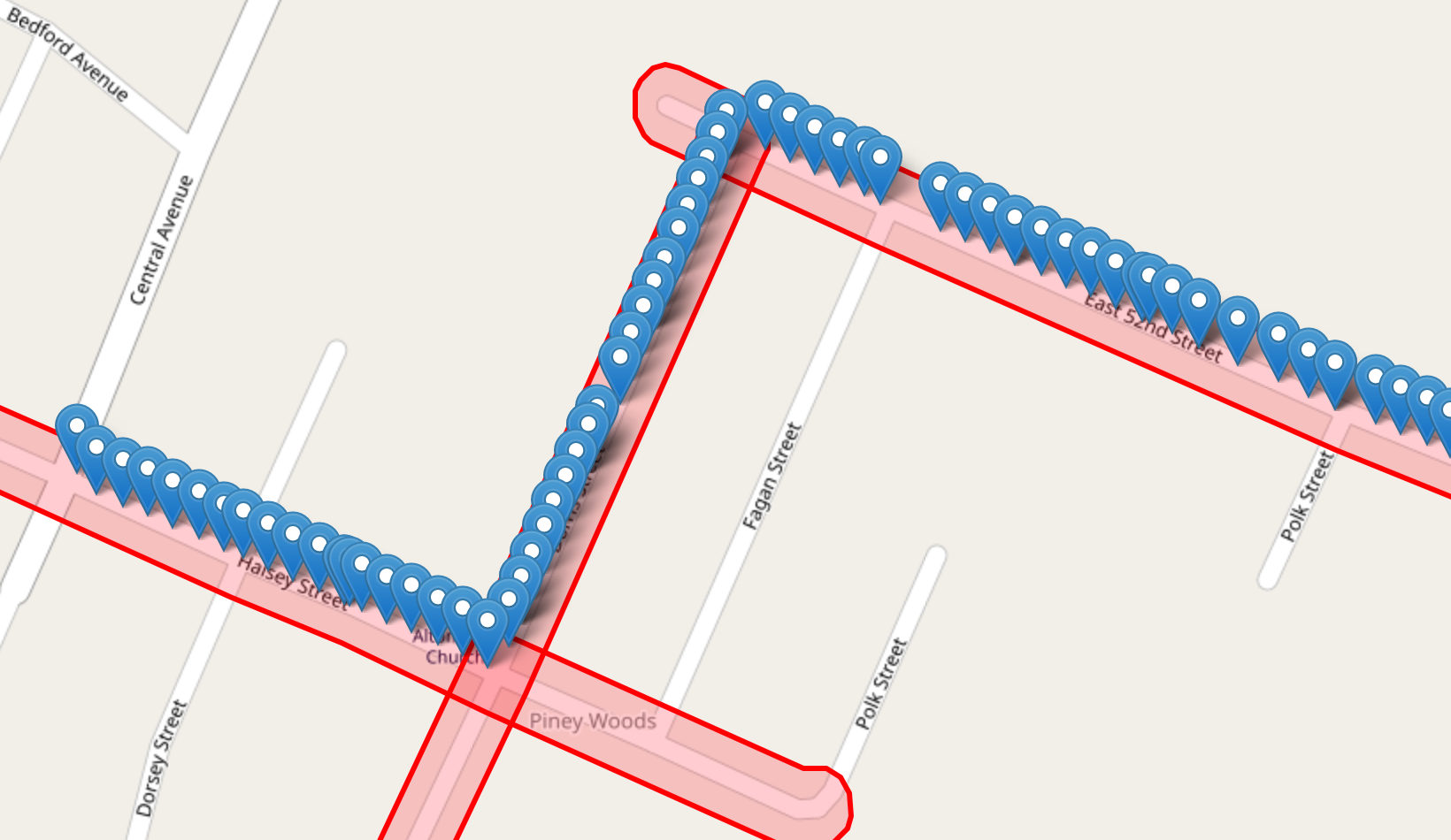
Figure 4: Mapping without noise.

Figure 5: Mapping with noise with 14-meter std. dev.

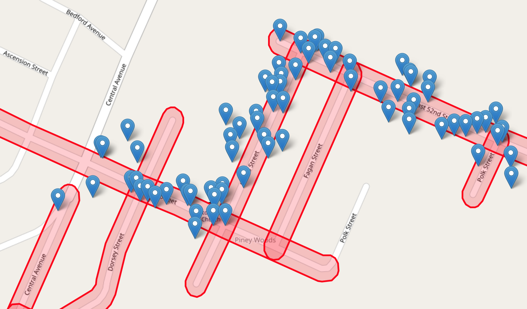
Figure 6: Mapping with noise with 28-meter std. dev.

Figures 6, 6 and 6 show locations with different levels of noise added, highlighting in red the road segments to which locations are mapped by Algorithm 1. Figure 7 shows the accuracy of mapping with various levels of noise, ranging from zero to 110-meter standard deviation in both directions. As expected, the accuracy of the algorithm decreases as the level of noise increases. However, for reasonable noise levels, it performs very well: with 14-meter standard deviation, it can still correctly map 84.5% of locations.

Figure 7: Accuracy of mapping noisy locations to road segments.

V-B Comparison of Weather, Traffic and Elevation Features

For both electric and diesel buses, we have a set of 26 features in each sample, besides energy use as the target feature. Now, we study which of these features are the most useful for predicting energy use, and which subset of features results in the lowest prediction error.

After preparing the samples for both electric and diesel buses, we randomly split them into training (80%) and test sets (20%). We use the same split ratio in all subsequent experiments. Since neural networks attain the lowest prediction error (see Section V-D), we compare features based on this model. We include vehicle-level data in all experiments, and try different combinations of weather, elevation, and traffic data.

(a) Electric

(b) Diesel

Figure 8: Prediction error with various sets of features. Note that electric and diesel energy are measured in different units.

color=yellow!5,linecolor=black!50]Aron: this should be a bar plot Figure 8(a) shows that elevation is by far the most significant feature for electric vehicles. Traffic data does improve prediction, but its impact is much smaller, especially if elevation is already included. This can be explained by regenerative breaking: the energy use of electric vehicles is not impacted by heavy traffic since they do not lose energy due to frequent braking. color=yellow!5,linecolor=black!50]Aron: this should be a bar plot On the other hand, Figure 8(b) shows that for diesel vehicles, both elevation and traffic data are significant, and both need to be included for good performance. Finally, we find that weather data has the lowest impact on prediction error for both electric and diesel vehicles.

V-C Comparison of Different Weather Features

Since weather data has many features, we also present a comparison among various weather features to see which ones help with prediction the most. We consider temperature (T), humidity (H), visibility (V), wind speed (W), and precipitation (P) in this comparison.

(a) Electric

(b) Diesel

Figure 9: Prediction error with various weather features.

Figure 9 shows prediction error with various combinations of weather features (with traffic and elevation always included). For electric vehicles, we attain lowest error when we use all five features together (Figure 9(a)). On the other hand, for diesel vehicles, we attain lowest error using only three features: temperature, visibility and precipitation (Figure 9(b)). This may be explained by over-fitting when using more features.

V-D Comparison of Prediction Models for Samples

We first evaluate the three machine-learning models based on how well they predict energy use for samples. Our samples represent segments of trips that are short in both distance and duration, presenting a challenging problem for prediction.

Figures 10 and 11 show mean squared error (MSE) and mean absolute error (MAE) for the three models. Based on MSE, the artificial neural network (ANN) outperforms the other two models for both electric and diesel vehicles. However, based on MAE, ANN outperforms decision trees (DT) for diesel vehicles but not for electric vehicles. Note that we optimized all models to minimize MSE, which can explain the slightly inferior performance of ANN for MAE. We have not encountered any overfitting since our training and testing errors were consistent for each model.

Figure 10: Mean square error (MSE) and mean absolute error (MAE) for electric vehicle samples.

Figure 11: Mean square error (MSE) and mean absolute error (MAE) for diesel vehicle samples.

V-E Comparison of Prediction Models for Longer Trips

Finally, we study how well our models perform with respect to predicting energy use for longer trips. First, we divide our time series into longer trips, varying the length of the trips between 10 minutes and 6 hours. For each trip, we generate a set of samples (as described in Section III), use our models to predict energy use for each sample, and then compare the sum of these predictions to the actual energy use of the trip.

Figure 12 shows the relative prediction error for trips of various lengths. For each length, we plot an average error value computed over many trips. We see that relative prediction error is generally lower for longer trips; this is expected as the individual errors of large numbers of samples cancel each other out with an unbiased prediction model. For diesel vehicles, we find that the ANN outperforms the other models significantly for all trip lengths. On the other hand, for electric vehicles, ANN and DT perform equally well for most trip lengths.

(a) Electric

(b) Diesel

Figure 12: Prediction error for longer trips with neural network (ANN), decision tree (DT), and linear regression (LR).

VI Related Work

Our study is most closely related to the work of Cauwer et al. and of Wickramanayake and Bandara. Cauwer et al. [16] use a cascade of ANN and multiple linear regression models as a data-driven energy-consumption prediction method for EVs. Their study uses vehicle monitoring data as time series of tuples for two types of vehicles with location, vehicle speed, and energy-consumption information, such as battery voltage, current, and SoC. Their dataset also includes road network data, weather data, and an altitude map. Our approach has some similarity to this study. However, we also use traffic data in our model, which we find to be very helpful with diesel prediction. Wickramanayake and Bandara [17] assess three different techniques for fuel consumption prediction of a long-distance public bus. Their time series tuples include GPS location, bearing, elevation, distance travelled, speed, acceleration, ignition status, battery voltage, fuel level, and fuel consumption. The authors compare the performance among two ensemble models, random forest and gradient boosting, and one ANN model. However, their study lacks critical parameters, such as road information, traffic, weather, etc.

Perrotta et al. [18] compare the performance of SVM, RF, and ANN in modelling fuel consumption of a large fleet of trucks. Their features include gross vehicle weight, speed, acceleration, geographical position, torque percentage, revolutions of the engine, activation of cruise control, use of brakes and acceleration pedal, measurement of travelled distance, fuel consumption. The study also combines some road characteristics. From the comparison of the RMSE, MAE, and R2 score of the prediction, RF gives the best performance. Nageshrao et al. [19] models the energy consumption of electric buses based on time-dependent factors such as ambient temperature and speed, battery capacity, total mass, battery parameters, etc. They use a NARX based ANN time series predictor to predict the state of charge of the battery. Gao et al. [20] discuss an adaptive wavelet neural network (WNN) based energy prediction. The study uses features such as day type, temperature, rainfall, the travelled distance, and clarity of the atmosphere. The study groups the trip days based on similar attributes, using Grey Relational Analysis (GRA) and then implements the Adaptive WNN.

Some researchers propose methods for optimizing the operations of vehicle fleets. Wang et al. [21] design a real-time charging scheduling system, called bCharge, for electric bus fleets. They implement the system with the real-world streaming dataset from Shenzhen, China, including GPS data, bus stop data, bus transaction lines, bus charging station data, and electricity rate data. Murphey et al. [22] propose the ML_EMO_HEV framework for energy management optimization in an hybrid-electric vehicles. Their framework first uses a ANN to model the road environment of a driving trip as a sequence of different roadway types and traffic congestion levels. Then, it uses an additional ANN to model the driver’s instantaneous reaction to the driving environment. Finally, the framework uses an additional set of ANN to emulate the optimal energy management strategy.

VII Discussion and Conclusion

We presented a framework for the data-driven prediction of the energy use of electric and internal-combustion vehicles, which we evaluated on real-world data collected from a transit fleet. Our results show that it is possible to collect, aggregate, and process heterogeneous transit data effectively. We found that generally, artificial neural networks perform best for predicting energy use. For diesel buses, we achieve best results using 21 predictor variables: travel distance, 14 road-type features, elevation change, 3 weather features, and 2 traffic features. For electric buses, we achieve best results using 23 predictor variables, which include 2 more weather features. We also found that relative prediction error is lower for longer trips, which facilitates the long-term planning of transit operations.

Acknowledgment

We thank the anonymous reviewers. This material is based upon work supported by the Department of Energy, Office of Energy Efficiency and Renewable Energy (EERE), under Award Number DE-EE 0008467.

References

- [1] EIA, “U.S. Energy Information Administration: Use of energy explained – energy use for transportation (2018),” https://www.eia.gov/energyexplained/use-of-energy/transportation.php, Accessed: February 14th, 2020, 2018.
- [2] Office of Transportation and Air Quality, “Fast facts: U.S. transportation sector greenhouse gas emissions 1990–2017,” Tech. Rep. EPA-420-F-19-047, June 2019. [Online]. Available: https://nepis.epa.gov/Exe/ZyPDF.cgi?Dockey=P100WUHR.pdf
- [3] Tennessee Dept. of Finance and Administration. (2019) Elevation data. [Online]. Available: https://www.tn.gov/finance/sts-gis/gis/data.html
- [4] USGS. (2019) The national map. [Online]. Available: https://pubs.er.usgs.gov/publication/fs20193032
- [5] Dark Sky, “API documentation,” https://darksky.net/dev/docs, Accessed: January 29th, 2020, 2019.
- [6] (2018) HERE API. [Online]. Available: https://developer.here.com/
- [7] (2018) Traffic Message Channel. [Online]. Available: https://wiki.openstreetmap.org/wiki/TMC
- [8] M. Zaharia, R. S. Xin, P. Wendell, T. Das, M. Armbrust, A. Dave, X. Meng, J. Rosen, S. Venkataraman, M. J. Franklin et al., “Apache Spark: A unified engine for big data processing,” Communications of the ACM, vol. 59, no. 11, pp. 56–65, 2016.
- [9] M. H. Iqbal and T. R. Soomro, “Big data analysis: Apache Storm perspective,” International journal of computer trends and technology, vol. 19, no. 1, pp. 9–14, 2015.
- [10] (2019) Apache Pulsar – An open-source distributed pub-sub messaging system. [Online]. Available: https://pulsar.apache.org/
- [11] (2019) Apache BookKeeper – A scalable, fault-tolerant, and low-latency storage service optimized for real-time workloads. [Online]. Available: https://bookkeeper.apache.org/
- [12] (2019) Apache ZooKeeper. [Online]. Available: https://zookeeper.apache.org/
- [13] (2019) MongoDB – the database for modern applications. [Online]. Available: https://www.mongodb.com/
- [14] D. P. Kingma and J. Ba, “Adam: A method for stochastic optimization,” arXiv preprint arXiv:1412.6980, 2014.
- [15] scikit learn, “Decision tree regressor,” https://scikit-learn.org/stable/modules/generated/sklearn.tree.DecisionTreeRegressor.html, Accessed: February 14th, 2020.
- [16] C. De Cauwer, W. Verbeke, T. Coosemans, S. Faid, and J. Van Mierlo, “A data-driven method for energy consumption prediction and energy-efficient routing of electric vehicles in real-world conditions,” Energies, vol. 10, no. 5, p. 608, 2017.
- [17] S. Wickramanayake and H. D. Bandara, “Fuel consumption prediction of fleet vehicles using machine learning: A comparative study,” in 2016 Moratuwa Engineering Research Conference (MERCon). IEEE, 2016, pp. 90–95.
- [18] F. Perrotta, T. Parry, and L. C. Neves, “Application of machine learning for fuel consumption modelling of trucks,” in 2017 IEEE International Conference on Big Data (Big Data). IEEE, 2017, pp. 3810–3815.
- [19] S. P. Nageshrao, J. Jacob, and S. Wilkins, “Charging cost optimization for EV buses using neural network based energy predictor,” IFAC-PapersOnLine, vol. 50, no. 1, pp. 5947–5952, 2017.
- [20] Y. Gao, S. Guo, J. Ren, Z. Zhao, A. Ehsan, and Y. Zheng, “An electric bus power consumption model and optimization of charging scheduling concerning multi-external factors,” Energies, vol. 11, no. 8, p. 2060, 2018.
- [21] G. Wang, X. Xie, F. Zhang, Y. Liu, and D. Zhang, “bCharge: Data-driven real-time charging scheduling for large-scale electric bus fleets,” in 2018 IEEE Real-Time Systems Symposium (RTSS), 2018, pp. 45–55.
- [22] Y. L. Murphey, J. Park, Z. Chen, M. L. Kuang, M. A. Masrur, and A. M. Phillips, “Intelligent hybrid vehicle power control–Part I: Machine learning of optimal vehicle power,” IEEE Transactions on Vehicular Technology, vol. 61, no. 8, pp. 3519–3530, 2012.