MLPSVM:A new parallel support vector machine to multi-label learning

Abstract

Multi-label learning has attracted the attention of the machine learning community. The problem conversion method Binary Relevance converts a familiar single label into a multi-label algorithm. The binary relevance method is widely used because of its simple structure and efficient algorithm. But binary relevance does not consider the links between labels, making it cumbersome to handle some tasks. This paper proposes a multi-label learning algorithm that can also be used for single-label classification. It is based on standard support vector machines and changes the original single decision hyperplane into two parallel decision hyperplanes, which call multi-label parallel support vector machine(MLPSVM).At the end of the article, MLPSVM is compared with other multi-label learning algorithms. The experimental results show that the algorithm performs well on data sets.

1 Introduction

Multi-label learning is widely used to serve our real life[1, 2, 3, 4, 5, 6]. In the field of music classification[7], traditional classification algorithms will classify music into pop and rock classes, which are too broad. Use multi-label learning algorithms to expand music classification to tasks with multiple labels will make music classification more in line with practical requirements. For protein chloroplast localization[5] in the biological field, the traditional method uses single-position protein chloroplast localization, but ignores multi-position protein chloroplast localization. Using multi-label learning to perform multi-position protein chloroplast localization has better effect. Studying multi-label learning algorithm will help to solve the existing problems. Zhang[8],has reviewed multi-label learning and introduced multi-label learning in detail. Multi-label learning algorithms are simply divided into the following two categories:

• Problem conversion methods:converts the multi-label learning problem into a familiar single label problem to solve the problem, such as the first-order method Binary Relevance and the high-order method Classifier Chains.

• Algorithm adaptive method: this kind of algorithm directly uses multi-label data to solve the multi-label problem. The representative algorithms are the first-order ML-KNN[9], ML-DT[10] second-order Rank-SVM[11], CML[12].

In multi-label learning, considering the association between labels, there will be label combination explosion[13] and redundant feature information[14]. Many multi-label learning algorithms are proposed[15, 16, 17, 18, 19, 20] to solve the above problems. For multi-label data, the data has both the same label and different labels, which will result in data crossing. It seems that few scholars pay attention to the situation of data crossing. Chen[21] proposed MLTSVM, which can handle crossing amount data well.

In this paper, a multi-label classification method based on support vector machine(SVM)[22] is designed call it MLPSVM. MLPSVM uses two parallel hyperplanes to identify a label. The use of MLPSVM will facilitate SVM to perform multi-label classification tasks. At the same time, MLPSVM is a convex quadratic programming model.

1.1 Notation and Setup

Let $X=R^{n}$ be the n-dimensional input space and $Y=R^{d}$ be the d-dimensional label space,where $y=(y_{1},y_{2},y_{3}...y_{d})\in\{1,-1\}^{d}$. Given a multi-label training set $D=\{(x_{i},y_{i})|1\leq i\leq m\}$,where $x_{i}\in X$ is a feature vector and $y_{i}\in Y$ is the set of label associateal with the $x_{i}$. The goal of MLPSVM is to obtain two matrices

$$w=\begin{bmatrix}w_{11}&w_{12}&w_{13}&\dots&w_{1n}\\ {5}\\ w_{j1}&w_{j2}&w_{j3}&\dots&w_{jn}\\ {5}\\ w_{d1}&w_{d2}&w_{d3}&\dots&w_{dn}\end{bmatrix},b=\begin{bmatrix}b_{11}&{b_{12}}\\ {2}\\ b_{j1}&b_{j2}\\ {2}\\ b_{d1}&b_{d2}\end{bmatrix},$$

$w_{j}$ is row j matrix $w$.For the input feature vector $x\in X$. The label $y=(y_{1},y_{2},y_{3}...y_{d})\in Y$ about $x$ is obtained by expression

$$y_{j}=\Bigg{\{}_{-1\ otherwise}^{+1\ f_{j1}=w_{j}x+b_{j1}\geq 0\ and\ f_{j2}=w_{j}x+b_{j2}\leq 0}.$$ (1)

2 Support Vector Machine

Support vector machine is a binary classification model. Its basic model is the linear classifier with the largest interval defined on the feature space. The learning strategy of support vector is to find a hyperplane in the sample space to separate the two classes at maximum intervals. We denote the set of training data as $T=\{(x_{i},y_{i})|1\leq i\leq m\}$ where $x_{i}\in R^{n}$ represents an input instance with the corresponding label $y_{i}\in\{1,-1\}$.The primal problem of SVM can be expressed as

$$\mathop{min}\limits_{w,b,\delta_{i}}\quad \frac{1}{2}\|w\|^{2}+c\sum\limits_{i=1}^{m}\delta_{i}$$

$$s.t.\quad y_{i}(wx_{i}+b)\geq 1-\delta{i},$$

$$\delta{i}\geq 0,i=1,2,...,m,$$ (2)

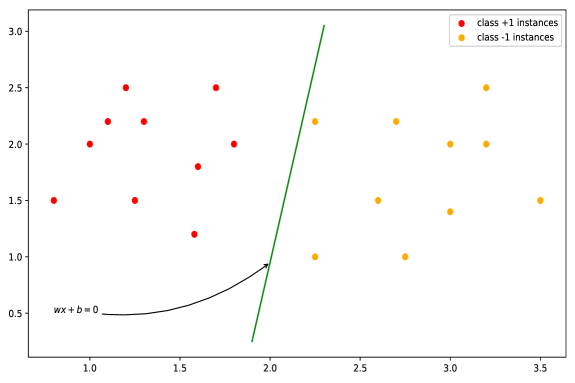
where $\delta_{i}$ is the slack variable to indicate the misclassification error,and $c>0$ is the penalty parameter. $w$ and $b$ are the normal vector and the bias term of hyperplanes respectively. An intuitive geometric interpretation for SVM is shown in 1.Formula 2 is a convex quadratic programming problem, $w$ and $b$ can be obtained by solving this problem.Therefore,the desision function $f(x)=sign(wx+b)$.

Figure 1: An intuitive geometric interpretation SVM

A new data instance $x$ ,the class $y={+1,-1}$ about x is obtained by expressed

$$y=\Bigg{\{}_{+1\ wx+b\geq 0.}^{-1\ wx+b<0}$$ (3)

Introducing kernel techniques into support vector machines can also make support vector machines nonlinear classifiers.

3 Multi label parallel support vector machine

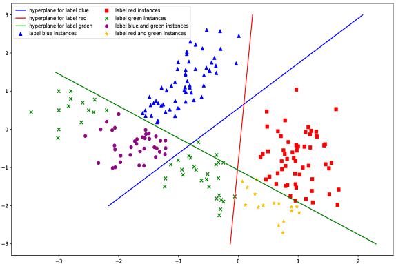
This section introduces multi-label parallel support vector machine. Considering the data intersection in the multi-label problem, a multi-label parallel support vector machine is designed to solve the problem. As shown in Figure 2, using BR_SVM will cause the data with only green labels on the left to be incorrectly predicted with blue labels.

Figure 2: An intuitive geometric interpretation BR_SVM

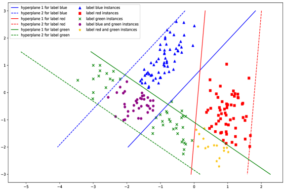
MLPSVM uses two parallel hyperplanes $f_{j1}(x)=w_{j}x+b_{j1}$ and $f_{j2}(x)=w_{j}x+b_{j2}$ to identify a tag. The goal is to locate the relevant tag data between the two hyperplanes. The function of hyperplane $f_{j1}$ is still the same as that of traditional support vector machine, which is responsible for separating different label data, so that for all sample data there are

$$y_{ij}(w_{j}x+b_{j1})\geq 1-\delta_{i}.$$ (4)

The hyperplane $f_{j2}$ is responsible for locating the corresponding data between the two hyperplanes $f_{j1}$ and $f_{j2}$. For data x, if $y_{ij}=+1$, there are $f_{j1}(x)\geq 0$, $f_{j2}(x)\leq 0$. Design the following constraints

$$(1+y_{ij})(w_{j}x+b_{j1})\leq 0.$$ (5)

Constraint (5) makes the corresponding data with positive label $y_{ij}=+1$ subject to the above constraint. For data with negative label $y_{ij}=-1$, because $(1+y_{ij})(w_{j}x+b_{j1})\leq 0$, this is an identity and will not be constrained. In order to enable hyperplanes $f_{j1}$ and $f_{j2}$ to tightly surround data, a relaxation variable is added in constraint 5, so that constraint (5) becomes an equality constraint

$$(1+y_{ij})(w_{j}x+b_{j1})+\alpha_{ij}=0.$$ (6)

The $\alpha_{ij}$ are slack variables measureing the distance that hyperplanes $f_{j2}$ makes on the data. Bring $\alpha_{ij}$ into the objective function, there are

$$\mathop{min}\limits_{w,b,\delta,\alpha}\frac{1}{2}\sum\limits_{j=1}^{d}\|{w_{j}}\|^{2}+C_{1}\sum\limits_{i=1}^{m}\sum\limits_{j=1}^{d}\delta_{ij}+C_{2}\sum\limits_{i=1}^{m}\sum\limits_{j=1}^{d}\alpha_{ij}$$ (7)

Figure 3: An intuitive geometric interpretation MLPSVM

In this way, MLPSVM will consider the distance of data to hyperplane $f_{j2}$.An intuitive geo-metric interpretation for MLPSVM is shown in Figure 3.

3.1 linear multi label parallel support vector machine

Now begin introduce parallel multi label support vector machine classifier by formulating the classification problem as:

$$\mathop{min}\limits_{w,b,\delta,\alpha}\quad\frac{1}{2} \sum\limits_{j=1}^{d}\|{w_{j}}\|^{2}+C_{1}\sum\limits_{i=1}^{m}\sum\limits_{j=1}^{d}\delta_{ij}+C_{2}\sum\limits_{i=1}^{m}\sum\limits_{j=1}^{d}\alpha_{ij}$$

$$s.t.\quad y_{ij}(w_{j}x_{i}+b_{j1})\geq 1-\delta_{ij}$$

$$(1+y_{ij})(w_{j}x_{i}+b_{j2})+\alpha_{ij}=0$$

$$\delta_{ij}\geq 0,\alpha_{ij}\geq 0$$

$$for\ i=1,...,m\ and\ j=1,...,d.$$ (8)

Figure 4: MLPSVM use two ratios $\frac{C_{1}}{C_{2}}$, for the same training data.

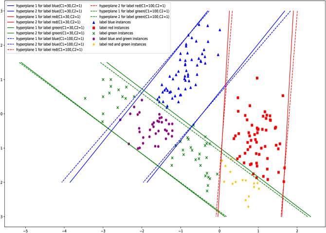
In this problem, $C_{1}$ and $C_{2}$ are regularization parameters. The $\delta_{ij}$ are slack variables measureing the error that hyperplanes $f_{j1}$ makes on the data. The $\alpha_{ij}$ are slack variables measureing the distance that hyperplanes $f_{j2}$ makes on the data. This constraint ? can only be applied to positive labels. For negative labels $y_{ij}=-1$,$(1+y_{ij})(w_{j}x_{i}+b_{j2})+\alpha_{ij}=0$ which is an identity. The emphasis of the model is adjusted by changing the value of the ratio $\frac{C_{1}}{C_{2}}$. The larger the ratio $\frac{C_{1}}{C_{2}}$, the better the hyperplane $f_{j1}$ can separate the positive training data from the negative training data. The smaller the ratio $\frac{C_{1}}{C_{2}}$, the closer the positive training data will be to the hyperplane $f_{j2}$. As show in Figure 4,use two ratios $\frac{C_{1}}{C_{2}}$, for the same training data.

According to the above model, observation shows that the model can be simplified,$\|{w_{j}}\|^{2}$ and $w_{j}x_{i}$ Appears in the model.$w_{j}$ is row j of matrix w. this will bring difficulties to the solution.Through the following expression

$$W=(w_{1},w_{2},w_{3},...,w_{d})$$ (9)

$$\Phi(x_{i},j)=(\underbrace{0,...,0}_{j-1},x,\underbrace{0,...,0}_{d-j})$$ (10)

where we have denoted by 0 the vector in $R^{d}$ whose coordinates are all zero.By construction we have that

$$\frac{1}{2}\sum\limits_{j=1}^{d}\|{w_{j}}\|^{2}=\frac{1}{2}\|{W}\|^{2}$$ (11)

$$w_{j}x_{i}=W\cdot\Phi(x_{i},j).$$ (12)

Combining equations (11),(12)and (8) respectively will yield the following formula

$$\mathop{min}\limits_{W,b,\delta,\alpha}\quad \frac{1}{2}\|{W}\|^{2}+C_{1}\sum\limits_{i=1}^{m}\sum\limits_{j=1}^{d}\delta_{ij}+C_{2}\sum\limits_{i=1}^{m}\sum\limits_{j=1}^{d}\alpha_{ij}$$

$$s.t.\quad y_{ij}(W\cdot\Phi(x_{i},j)+b_{j1})\geq 1-\delta_{ij}$$

$$(1+y_{ij})(W\cdot\Phi(x_{i},j)+b_{j2})+\alpha_{ij}=0$$

$$\delta_{ij}\geq 0,\alpha_{ij}\geq 0$$

$$for\ i=1,...,m\ and\ j=1,...,d$$ (13)

The new expression obtained is similar to the standard SVM expression. At the same time, it can be easily seen that this is a convex quadratic programming problem.

3.2 Dual Optimization Problem

An importtant characteristic of SVM is that they can be used to estimate highly non-linear functions through the use of kernels. In the section,derive the dual of problem (13).The Lagrangian with $\eta_{ij}\geq 0,\lambda_{ij}\geq 0,\mu_{ij}\geq 0$ of (13) is

$$L(W,b,\delta,\alpha,\eta,\theta,\lambda,\mu)= \frac{1}{2}\|{W}\|^{2}+C_{1}\sum\limits_{i=1}^{m}\sum\limits_{j=1}^{d}\delta_{ij}+C_{2}\sum\limits_{i=1}^{m}\sum\limits_{j=1}^{d}\alpha_{ij}$$

$$-\sum\limits_{i=1}^{m}\sum\limits_{j=1}^{d}\eta_{ij}(y_{ij}(W\cdot\Phi(x_{i},j)+b_{j1})-1+\delta_{ij})$$

$$+\sum\limits_{i=1}^{m}\sum\limits_{j=1}^{d}\theta_{ij}((1+y_{ij})(W\cdot\Phi(x_{i},j)+b_{j2})+\alpha_{ij})$$

$$-\sum\limits_{i=1}^{m}\sum\limits_{j=1}^{d}\lambda_{ij}\delta_{ij}-\sum\limits_{i=0}^{m}\sum\limits_{j=0}^{d}\mu_{ij}\alpha_{ij}.$$ (14)

Then according to

$$\frac{\partial L}{\partial W}=W-\sum\limits_{i=1}^{m}\sum\limits_{j=1}^{d}\eta_{ij}y_{ij}\Phi(x_{i},j)+\sum\limits_{i=1}^{m}\sum\limits_{j=1}^{d}\theta_{ij}(1+y_{ij})\Phi(x_{i},j)=0$$ (15)

$$\frac{\partial L}{\partial b_{j1}}=-\sum\limits_{i=1}^{m}\eta_{ij}y_{ij}=0,\forall j=1,...,d$$ (16)

$$\frac{\partial L}{\partial b_{j2}}=-\sum\limits_{i=1}^{m}\theta_{ij}(1+y_{ij})=0,\forall j=1,...,d$$ (17)

$$\frac{\partial L}{\partial\delta_{ij}}=C_{1}-\eta_{ij}-\lambda_{ij}=0,\forall i=1,...,m,\forall j=1,...,d$$ (18)

$$\frac{\partial L}{\partial\alpha_{ij}}=C_{2}+\theta_{ij}-\mu_{ij}=0,\forall i=1,...,m,\forall j=1,...,d$$ (19)

the dual problem of (13) is obtained as follows,

$$\mathop{max}\limits_{\eta,\theta}\ -\frac{1}{2}\sum\limits_{i=1}^{m}\sum\limits_{k=1}^{m}\sum\limits_{j=1}^{d}\eta_{ij}\eta_{kj}y_{ij}y_{kj}\Phi(x_{i},j)\cdot\Phi(x_{k},j)$$

$$+\sum\limits_{i=1}^{m}\sum\limits_{k=1}^{m}\sum\limits_{j=1}^{d}\eta_{ij}\theta_{kj}y_{ij}(1+y_{kj})\Phi(x_{i},j)\cdot\Phi(x_{k},j)$$

$$+\frac{1}{2}\sum\limits_{i=1}^{m}\sum\limits_{k=1}^{m}\sum\limits_{j=1}^{d}\theta_{ij}\theta_{kj}(1+y_{ij})(1+y_{kj})\Phi(x_{i},j)\cdot\Phi(x_{k},j)$$

$$+\sum\limits_{i=1}^{m}\sum\limits_{j=1}^{d}\eta_{ij}$$

$$s.t. \sum\limits_{i=1}^{m}\eta_{ij}y_{ij}=0,\forall j=1,...,d$$

$$\sum\limits_{i=1}^{m}\theta_{ij}(1+y_{ij})=0,\forall j=1,...,d$$

$$0\leq\eta_{ij}\leq C_{1},for\ i=1,...,m\ and\ j=1,...,d.$$ (20)

If the solution to the above problem is $(\eta_{11},...,\eta_{ij},...,\eta_{md},\theta_{11},...,\theta_{ij},...,\theta_{md})$ where is $\eta_{ij}\geq 0,y_{kj}=1\ and\ \theta_{kj}\neq-C_{2}$ ,the solution of $(W,b)$ can be calculated as following:

$$W= \sum\limits_{i=1}^{m}\sum\limits_{j=1}^{d}\eta_{ij}y_{ij}\Phi(x_{i},j)+\sum\limits_{i=1}^{m}\sum\limits_{j=1}^{d}\theta_{ij}(1+y_{ij})\Phi(x_{i},j)$$ (21)

$$b_{j1}= y_{ij}-W\cdot\Phi(x_{i},j),\forall j=1,...,d$$ (22)

$$b_{j2}= -(1+y_{ij})(W\cdot\Phi(x_{i},j)),\forall j=1,...,d$$ (23)

3.3 Non linear parallel multi label support vector machine

One of the characteristics of support vector machines which is widely used is that they can be used to estimate nonlinear functions. We can clearly generalize the linear PMLSVM method outlined above to the non-linear case using kernels as is done for SVM. We define nonlinear feature map

$$\emptyset\ :\Phi(x_{i},j)\rightarrow H$$ (24)

where $H$ is a separable Hilbert space.The kernel associated to $\emptyset$ is

$$K(\Phi(x_{i},j),\Phi(x_{k},s))=<\emptyset(\Phi(x_{i},j)),\emptyset(\Phi(x_{k},s))>$$ (25)

where $<.,.>$ is the inner product in $H$.The kernel method is introduced into the dual problem to obtain

$$\mathop{max}\limits_{\eta,\theta}\ -\frac{1}{2}\sum\limits_{i=1}^{m}\sum\limits_{k=1}^{m}\sum\limits_{j=1}^{d}\eta_{ij}\eta_{kj}y_{ij}y_{kj}K(\Phi(x_{i},j)\cdot\Phi(x_{k},j))$$

$$+\sum\limits_{i=1}^{m}\sum\limits_{k=1}^{m}\sum\limits_{j=1}^{d}\eta_{ij}\theta_{kj}y_{ij}(1+y_{kj})K(\Phi(x_{i},j)\cdot\Phi(x_{k},j))$$

$$+\frac{1}{2}\sum\limits_{i=1}^{m}\sum\limits_{k=1}^{m}\sum\limits_{j=1}^{d}\theta_{ij}\theta_{kj}(1+y_{ij})(1+y_{kj})K(\Phi(x_{i},j)\cdot\Phi(x_{k},j))$$

$$+\sum\limits_{i=1}^{m}\sum\limits_{j=1}^{d}\eta_{ij}$$

$$s.t. \sum\limits_{i=1}^{m}\eta_{ij}y_{ij}=0,\forall j=1,...,d$$

$$\sum\limits_{i=1}^{m}\theta_{ij}(1+y_{ij})=0,\forall j=1,...,d$$

$$0\leq\eta_{ij}\leq C_{1},for\ i=1,...,m\ and\ j=1,...,d$$ (26)

4 Experiments

4.1 Experimental setup

To evaluate the performance of MLPSVM,in this section we investigate its performance on real-world datasets. As a comparison, we compare MLPSVM with other five multi-label classifiers. Including MLKNN[9],MLARAM[23],BR_SVM,CC_SVM[24],MLTSVM[21]. In order to evaluate the performance of the algorithm, we select the following four metrics including Hmloss(Hamming loss),Oerr(One-error),Pre(Precision),Rec(Recall). Let’s introduce these four metrics.

• Hamming loss: Evaluates how many times an instance-label pair is misclassified between the pre dicted label set $h(x)$ and the ground-truth label set y

  $$Hmloss(h)=\frac{1}{p}\sum\limits_{i=1}^{p}\frac{1}{k}|h(x_{i})\Delta y_{i}|\in[0,1],$$ (27)

  where $\delta$ stands for the symmetric difference of two sets.
  

• One-error:Evaluate the number of times top-ranked label is not in the sample’s real label set the smaller the value, the better the performance.

  $$one-error(h)=\frac{1}{p}\sum\limits_{i=1}^{p}h(x_{i})\in[0,1],h(x_{i})=\bigg{\{}_{1\ otherwise}^{0\ if\ argmaxf_{y}(x_{i})\in y_{i}}$$ (28)

• Precision,Recall:

  $$Precision(h)=\frac{1}{p}\sum\limits_{i=1}^{p}\frac{|Y_{i}\cap h(x_{i})|}{|h(x_{i})|}$$ (29)

  $$Recall(h)=\frac{1}{p}\sum\limits_{i=1}^{p}\frac{|Y_{i}\cap h(x_{i})|}{|Y_{i}|}$$ (30)

All the experiments are done on personal computers with an Intel Core-i5 7400 processor(3.00GHz) and 8 GB random access memory(RAM). All comparison algorithms are from python’s third repository Scikit-Multilearn[25]. We selected two continuous data sets from MULAN[26] multi-label learning librarie.As shown in Table1. These datasets represent a wide range of domains(audio,image,biology and music).

Table 1: Real world dataset introduction from MULAN multi-label learning open source library

Dataset	Domain	Instances	Features	Labels
CAL500	music	502	68	174
Scene	image	2407	294	6
Birds	audio	645	258	21-1
Yeast	biology	2417	103	14
Emotions	music	593	72	6

4.2 Results on real world datasets

In this section, linear MLPSVM is compared with other multi-label learning algorithms. In contrast, other algorithm that use SVM as that base classifier will also use linear SVM. Table 2,3,4,5 and 6 show the experimental results. The experimental results show that MLPSVM performs well on Emotions and Yeast data sets,which may be the cross distribution of data. The performance of MLPSVM on one_error evaluation index is obviously better than other algorithms.

Table 2: Results of Multi-label Classification Algorithm on CAL500 Data

	CAL500
Algithms	Hmloss	Oerr	Pre	Arc
MLPSVM	0.141$\pm$0.003	0.002$\pm$0.018	0.572 $\pm$0.018	0.223$\pm$0.010
MlARAM	0.181$\pm$0.019	0.388$\pm$0.124	0.376 $\pm$0.134	0.203$\pm$0.069
MLkNN	0.145$\pm$0.005	0.140$\pm$0.060	0.530 $\pm$0.029	0.264$\pm$0.020
MLTSVM	0.196$\pm$0.006	_	0.103 $\pm$0.026	0.040$\pm$0.010
BR_SVM	0.137$\pm$0.004	0.115 $\pm$0.051	0.618 $\pm$0.021	0.226$\pm$0.009
CC_SVM	0.137$\pm$0.004	0.145 $\pm$0.034	0.613 $\pm$0.013	0.223$\pm$0.006

Table 3: Results of Multi-label Classification Algorithm on Emotions Data

	Emotions
Algithms	Hmloss	Oerr	Pre	Arc
MLPSVM	0.213 $\pm$0.015	0.062 $\pm$ 0.024	0.698 $\pm$ 0.039	0.576 $\pm$ 0.034
MLARAM	0.363 $\pm$ 0.032	0.531 $\pm$ 0.078	0.422 $\pm$ 0.051	0.396 $\pm$ 0.056
MLkNN	0.265 $\pm$ 0.021	0.371 $\pm$ 0.043	0.604 $\pm$ 0.054	0.440 $\pm$ 0.049
MLTSVM	0.243 $\pm$ 0.011	_	0.645 $\pm$ 0.029	0.495 $\pm$ 0.030
BR_SVM	0.244 $\pm$ 0.026	0.344 $\pm$ 0.042	0.664 $\pm$ 0.062	0.438 $\pm$ 0.049
CC_SVM	0.240 $\pm$ 0.035	0.355 $\pm$ 0.060	0.673 $\pm$0.071	0.452 $\pm$ 0.074

Table 4: Results of Multi-label Classification Algorithm on Birds Data

	Birds
Algithms	Hmloss	Oerr	Pre	Arc
MLPSVM	0.062 $\pm$ 0.007	0.003 $\pm$ 0.006	0.396 $\pm$ 0.110	0.256 $\pm$ 0.066
MLARAM	0.079 $\pm$ 0.005	0.523 $\pm$ 0.046	0.462 $\pm$ 0.061	0.352 $\pm$ 0.032
MLkNN	0.053 $\pm$ 0.006	0.014 $\pm$ 0.013	0.876 $\pm$ 0.067	0.341 $\pm$ 0.025
MLTSVM	0.194 $\pm$ 0.017	_	0.158 $\pm$ 0.017	0.367 $\pm$ 0.032
BR_SVM	0.056 $\pm$ 0.007	0.101 $\pm$ 0.039	0.818 $\pm$ 0.068	0.320 $\pm$ 0.018
CC_SVM	0.056 $\pm$ 0.007	0.104 $\pm$ 0.028	0.812 $\pm$ 0.061	0.321 $\pm$ 0.028

Table 5: Results of Multi-label Classification Algorithm on Scene Data

	Scene
Algithms	Hmloss	Oerr	Pre	Arc
MLPSVM	0.173 $\pm$ 0.010	0.035 $\pm$ 0.017	0.532 $\pm$ 0.046	0.420 $\pm$ 0.039
MLARAM	0.115 $\pm$ 0.011	0.227 $\pm$ 0.040	0.643 $\pm$ 0.025	0.820 $\pm$ 0.036
MLkNN	0.092 $\pm$ 0.006	0.208 $\pm$ 0.031	0.782 $\pm$ 0.024	0.684 $\pm$ 0.036
MLTSVM	0.164 $\pm$ 0.009	_	0.569 $\pm$ 0.037	0.392 $\pm$ 0.031
BR_SVM	0.142 $\pm$ 0.005	0.531 $\pm$ 0.039	0.953 $\pm$ 0.034	0.226 $\pm$ 0.036
CC_SVM	0.137 $\pm$ 0.007	0.447 $\pm$ 0.047	0.942 $\pm$ 0.033	0.262 $\pm$ 0.034

Table 6: Results of Multi-label Classification Algorithm on Yeast Data

	Yeast
Algithms	Hmloss	Oerr	Pre	Arc
MLPSVM	0.187 $\pm$ 0.010	0.062 $\pm$ 0.019	0.712 $\pm$ 0.026	0.570 $\pm$ 0.020
MLARAM	0.217 $\pm$ 0.010	0.300 $\pm$ 0.023	0.653 $\pm$ 0.023	0.606 $\pm$ 0.019
MLkNN	0.199 $\pm$ 0.010	0.248 $\pm$ 0.022	0.706 $\pm$ 0.022	0.589 $\pm$ 0.015
MLTSVM	0.311 $\pm$ 0.004	_	0.408 $\pm$ 0.035	0.060 $\pm$ 0.012
BR_SVM	0.225 $\pm$ 0.008	0.389 $\pm$ 0.032	0.755 $\pm$ 0.025	0.378 $\pm$ 0.013
CC_SVM	0.236 $\pm$ 0.007	0.380 $\pm$ 0.055	0.696 $\pm$ 0.031	0.394 $\pm$ 0.022

5 Discussion

MLPSVM provides a new idea for processing multi-label data. Applying MLPSVM to real data sets, the results show that MLPSVM has better effect on Emotions and Yeast data sets. At the same time, the results show that MLPSVM performs poorly on Birds and Scene data sets. Experiments show that MLPSVM can process specific data well.After analysis MLPSVM has the following two areas to be improved:

• MLPSVM uses two hyperplanes, which will degrade the performance when the distribution of training samples is not true.

• A fast solution method for MLPSVM has not been found, which will limit MLSVM to solve large-scale problems.

References

- [1] Floriane Montanari, Barbara Zdrazil, Daniela Digles, and Gerhard F. Ecker. Selectivity profiling of bcrp versus p-gp inhibition: from automated collection of polypharmacology data to multi-label learning. Journal of Cheminformatics, 8(1):7, 2016.
- [2] C Mercan, S Aksoy, E Mercan, L. G. Shapiro, D. L. Weaver, and J. G. Elmore. Multi-instance multi-label learning for multi-class classification of whole slide breast histopathology images. IEEE Trans Med Imaging, PP(99):1–1, 2017.
- [3] Shibiao Wan, Man Wai Mak, and Sun Yuan Kung. Mem-adsvm: A two-layer multi-label predictor for identifying multi-functional types of membrane proteins. Journal of Theoretical Biology, 398:32–42, 2016.
- [4] Xiaotong Guo, Fulin Liu, Ying Ju, Zhen Wang, and Chunyu Wang. Human protein subcellular localization with integrated source and multi-label ensemble classifier. Scientific Reports, 6(1):28087, 2016.
- [5] S. Wan, M. W. Mak, and S. Y. Kung. Transductive learning for multi-label protein subchloroplast localization prediction. IEEE/ACM Transactions on Computational Biology & Bioinformatics, 14(1):212–224, 2017.
- [6] J. Zhang, Z. Zhang, Z. Wang, Y. Liu, and L. Deng. Ontological function annotation of long non-coding rnas through hierarchical multi-label classification. Bioinformatics, 34(10), 2018.
- [7] Sergio Oramas, Oriol Nieto, Francesco Barbieri, and Xavier Serra. Multi-label music genre classification from audio, text, and images using deep features. 2017.
- [8] Min-Ling Zhang and Zhi-Hua Zhou. A review on multi-label learning algorithms. IEEE transactions on knowledge and data engineering, 26(8):1819–1837, 2013.
- [9] Min-Ling Zhang and Zhi-Hua Zhou. Ml-knn: A lazy learning approach to multi-label learning. Pattern recognition, 40(7):2038–2048, 2007.
- [10] Amanda Clare and Ross D. King. Knowledge discovery in multi-label phenotype data. Lecture Notes in Computer Science, 2168(2168):42–53, 2001.
- [11] Andr E Elisseeff and Jason Weston. A kernel method for multi-labelled classification. In International Conference on Neural Information Processing Systems: Natural & Synthetic, 2001.
- [12] Nadia Ghamrawi and Andrew Mccallum. Collective multi-label classification. 2005.
- [13] M. L. Zhang, Kun Zhang, B. Rao, B. Krishnapuram, and Q. Yang. Multi-label learning by exploiting label dependency. In Acm Sigkdd International Conference on Knowledge Discovery & Data Mining, 2010.
- [14] Suping Xu, Xibei Yang, Hualong Yu, Dong Jun Yu, Jingyu Yang, and Eric C. C. Tsang. Multi-label learning with label-specific feature reduction. Journal of Computer Applications, 104:52–61, 2016.
- [15] Jesse Read, Luca Martino, and Jaakko Hollmén. Multi-label methods for prediction with sequential data. Pattern Recognition, 63:45–55, 2017.
- [16] Yue Zhu, Kai Ming Ting, and Zhi Hua Zhou. Multi-label learning with emerging new labels. In IEEE International Conference on Data Mining, 2017.
- [17] Rohit Babbar and Bernhard Schölkopf. Dismec: Distributed sparse machines for extreme multi-label classification. In Tenth Acm International Conference on Web Search & Data Mining, 2017.
- [18] Pawel Trajdos and Marek Kurzynski. Weighting scheme for a pairwise multi-label classifier based on the fuzzy confusion matrix. Pattern Recognition Letters, 103:60 – 67, 2018.
- [19] A. Mahdavi-Shahri, M. Houshmand, M. Yaghoobi, and M. Jalali. Applying an ensemble learning method for improving multi-label classification performance. In 2016 2nd International Conference of Signal Processing and Intelligent Systems (ICSPIS), pages 1–6, Dec 2016.
- [20] Joo Er Meng, Rajasekar Venkatesan, and Wang Ning. An online universal classifier for binary, multi-class and multi-label classification. In IEEE International Conference on Systems, 2017.
- [21] Wei-Jie Chen, Yuan-Hai Shao, Chun-Na Li, and Nai-Yang Deng. Mltsvm: a novel twin support vector machine to multi-label learning. Pattern Recognition, 52:61–74, 2016.
- [22] Corinna Cortes and Vladimir Vapnik. Support-vector networks. Machine learning, 20(3):273–297, 1995.
- [23] F. Benites and E. Sapozhnikova. Haram: A hierarchical aram neural network for large-scale text classification. pages 847–854, Nov 2015.
- [24] Jesse Read, Bernhard Pfahringer, Geoff Holmes, and Eibe Frank. Classifier chains for multi-label classification. In Joint European Conference on Machine Learning and Knowledge Discovery in Databases, pages 254–269. Springer, 2009.
- [25] P. Szymański and T. Kajdanowicz. A scikit-based Python environment for performing multi-label classification. ArXiv e-prints, February 2017.
- [26] Grigorios Tsoumakas, Ioannis Katakis, and Ioannis Vlahavas. Mining multi-label data. 2009.