The H₂O Spectrum of the Massive Protostar AFGL 2136 IRS 1 from 2 to 13 $\mu$m at High Resolution: Probing the Circumstellar Disk

Abstract

We have observed the massive protostar AFGL 2136 IRS 1 in multiple wavelength windows in the near-to-mid-infrared at high ($\sim 3$ km s^-1) spectral resolution using VLT+CRIRES, SOFIA+EXES, and Gemini North+TEXES. There is an abundance of H₂O absorption lines from the $\nu_{1}$ and $\nu_{3}$ vibrational bands at 2.7 $\mu$m, from the $\nu_{2}$ vibrational band at 6.1 $\mu$m, and from pure rotational transitions near 10–13 $\mu$m. Analysis of state-specific column densities derived from the resolved absorption features reveals that an isothermal absorbing slab model is incapable of explaining the relative depths of different absorption features. In particular, the strongest absorption features are much weaker than expected, indicating optical depth effects resulting from the absorbing gas being well-mixed with the warm dust that serves as the “background” continuum source at all observed wavelengths. The velocity at which the strongest H₂O absorption occurs coincides with the velocity centroid along the minor axis of the compact disk in Keplerian rotation recently observed in H₂O emission with ALMA. We postulate that the warm regions of this dust disk dominate the continuum emission at near-to-mid infrared wavelengths, and that H₂O and several other molecules observed in absorption are probing this disk. Absorption line profiles are not symmetric, possibly indicating that the warm dust in the disk that produces the infrared continuum has a non-uniform distribution similar to the substructure observed in 1.3 mm continuum emission.

1 Introduction

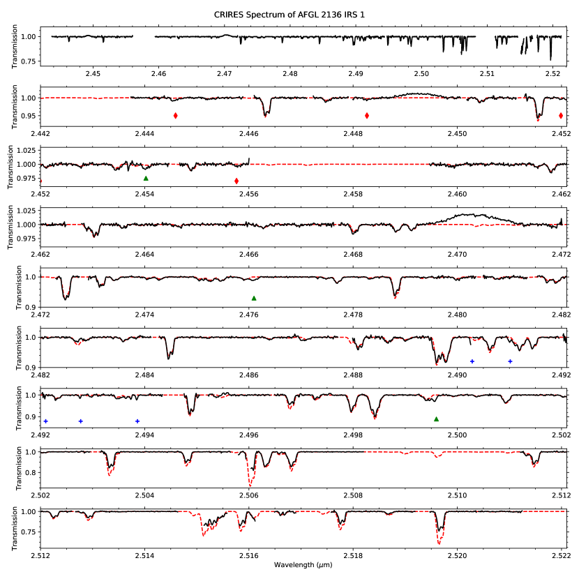
Figure 1: Shown here is the near infrared spectrum of AFGL 2136 IRS 1 obtained with CRIRES. The top panel shows the full coverage from about 2.442 $\mu$m to 2.522 $\mu$m, and the remaining panels zoom in on regions that are 0.01 $\mu$m wide. The two largest gaps are due to gaps in wavelength coverage between the CRIRES detectors. The smaller gaps are regions where poor atmospheric transmission precludes any useful analysis. The dashed red curve is the simulated H₂O absorption spectrum discussed in Section 4.3.1. Green triangles below the spectra mark HF absorption features, and blue crosses the unidentified features. Red diamonds in the second and third panels mark the locations of the CO $v=2$–0 $P(34)$, $P(35)$, $P(36)$, and $P(37)$ transitions. All remaining absorption features are caused by H₂O, while the broad emission features are due to the Pfund series of atomic H. All narrow “emission” features are artifacts of the telluric standard division process.

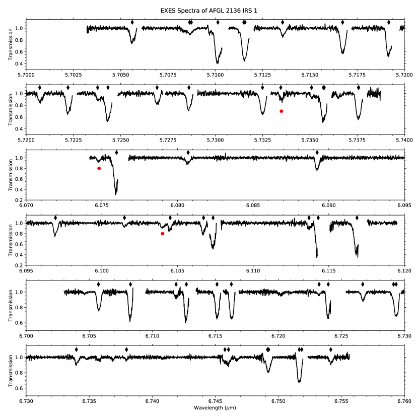
Figure 2: Shown here are the mid infrared spectra of AFGL 2136 IRS 1 in select regions from 5.7-6.8 $\mu$m obtained with EXES. Black diamonds above the spectra mark absorption features due to H₂O, and red circles beneath the spectra mark features due to H${}_{2}^{18}$O. There are some potentially unidentified features near 6.735 $\mu$m.

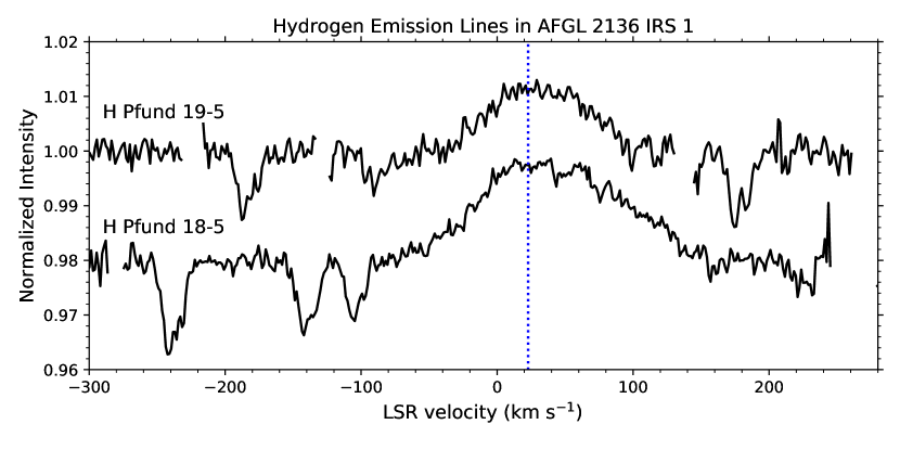
Figure 10: These spectra focus on the hydrogen Pfund emission lines observed toward AFGL 2136 IRS 1. The vertical dashed line marks the systemic velocity of 22.8 km s^-1.

AFGL 2136 IRS 1 (also referred to as CRL 2136, G17.64+0.16, and IRAS 18196$-$1331) is a luminous ($1.0\times 10^{5}$ L_☉; Lumsden et al., 2013) high mass ($45\pm 10$ M_☉; Maud et al., 2019) protostar that is believed to be in the latter stages of its evolution due to a variety of observed characteristics (Boonman & van Dishoeck, 2003; Maud et al., 2018, and references therein). It is located at a distance of 2.2 kpc away from the Sun (Urquhart et al., 2014), and has been extensively observed from centimeter to micron wavelengths, at low and high angular resolution, and low and high spectral resolution. The myriad observations paint a picture where a single, isolated massive protostar is driving a wide angle bipolar outflow through its natal cloud. The large scale outflow is observed in CO emission at millimeter wavelengths, with both the red and blue lobes being about 100″ in extent (Kastner et al., 1994; Maud et al., 2018). Closer to the central source (2″–10″) the outflow cavity walls are seen in scattered light at near infrared wavelengths (Kastner et al., 1992; Murakawa et al., 2008; Maud et al., 2018). The cool molecular envelope exhibits ice and dust absorption bands (Willner et al., 1982; Keane et al., 2001b; Dartois et al., 2002; Gibb et al., 2004), as well as molecular emission at millimeter wavelengths (van der Tak et al., 2000a, b), but a much warmer component is also inferred from several different molecules seen in absorption in the near-to-mid infrared (Mitchell et al., 1990; Lahuis & van Dishoeck, 2000; Keane et al., 2001a; Boonman & van Dishoeck, 2003; Boonman et al., 2003; Goto et al., 2013; Indriolo et al., 2013a; Goto et al., 2019). The presence of a dust disk on small spatial scales was suggested by near infrared polarization imaging (Minchin et al., 1991; Murakawa et al., 2008), and by mid infrared interferometric observations (de Wit et al., 2011; Boley et al., 2013). A compact source was marginally resolved at centimeter wavelengths along with a cluster of nearby 22 GHz H₂O masers (Menten & van der Tak, 2004), but only with the recent ALMA 1.3 mm continuum observations has the $93\times 71$ mas dust disk been fully resolved (Maud et al., 2019). Thermal line emission at 232.687 GHz from the H₂O $\nu_{2}=1$–1, 5_5,0-6_4,3 transition has the same spatial extent as the dust emission, and the H₂O gas velocities indicate Keplerian rotation within the disk (Maud et al., 2019). It is ideal that the reader has a clear picture of the AFGL 2136 region in mind to best understand the discussion throughout this paper. In particular, Figure 10 of Maud et al. (2018) provides an up-to-date schematic diagram of the AFGL 2136 region, and Figures 1 and 2 of Maud et al. (2019) present the compact disk observed in dust and gas emission, respectively.

The presence of circumstellar disks around massive protostars has important implications for the formation of high mass stars. The high luminosities ($\gtrsim 10^{5}$ L_☉) of massive protostars ionize and evaporate the surrounding molecular cloud, so it is thought that continued accretion onto the central source must be facilitated through disk-like structures (e.g., Krumholz et al., 2009; Klassen et al., 2016). Spectroscopic observations in the near and mid infrared provide the capability to measure molecular column densities in this accretion disk. By observing transitions out of several different rotational states of the same molecule, it becomes possible to constrain conditions such as the gas temperature, gas density, and radiation field in the gas where that molecule resides. We have previously demonstrated that H₂O is an excellent molecule for this purpose due to its large number of strong absorption lines at near-to-mid infrared wavelengths observed in massive protostars (Indriolo et al., 2013a, 2015). Here, we present the first analysis of H₂O absorption at high spectral resolution that combines observations from near-to-mid infrared wavelengths toward AFGL 2136 IRS 1. Such an analysis is instructive for future observations with the James Webb Space Telescope, where spectrally unresolved H₂O absorption will be detected throughout the infrared.

2 Observations

In order to perform high resolution spectroscopy from the near to mid-infrared we utilized three different instrument+telescope combinations: the Cryogenic High-resolution Infrared Echelle Spectrograph (CRIRES; Käufl et al., 2004) on UT1 at the Very Large Telescope provided coverage near 2.5 $\mu$m; the Echelon-Cross-Echelle Spectrograph (EXES; Richter et al., 2018) on board the Stratospheric Observatory for Infrared Astronomy (SOFIA; Young et al., 2012) provided coverage near 6 $\mu$m; and the Texas Echelon Cross Echelle Spectrograph (TEXES; Lacy et al., 2002) at Gemini North provided coverage near 12 $\mu$m. A log of the observations is presented in Table 1, and some further details regarding the execution at each observatory are given here.

2.1 CRIRES Observations

CRIRES observations targeting the $\nu_{1}$ and $\nu_{3}$ ro-vibrational bands of H₂O were made at two reference wavelengths: 2480.0 nm and 2502.8 nm. Due to the lack of a bright natural guide star near AFGL 2136, the adaptive optics system was not utilized. The 0$\farcs$2 slit was employed, providing a spectral resolving power of about $10^{5}$, corresponding to $\sim 3$ km s^-1 resolution. The slit was oriented at a position angle of 45^∘ (along a northeast-to-southwest axis) to minimize contamination from the near-IR scattered light observed in the region (e.g., Murakawa et al., 2008). Spectra were obtained in an ABBA pattern along the slit with 10″ between the two nod positions and $\pm 3$″ jitter width. All observations of AFGL 2136 IRS 1 were immediately preceeded by observations of the bright A2IV star HR 6378 using the same setup for use as a telluric standard.

2.2 EXES Observations

EXES observations targeting the $\nu_{2}$ ro-vibrational band of H₂O were made in cross-dispersed high-resolution mode targeting central wavenumbers of 1485.24 cm^-1, 1639.29 cm^-1, and 1747.25 cm^-1 (hereafter referred to as the 6.7 $\mu$m, 6.1 $\mu$m, and 5.7 $\mu$m spectra, respectively). The entrance slit had a width of 1$\farcs$84, providing a resolving power (resolution) of $\sim 85$,000 (3.5 km s^-1), and a length of about 10″ (varies slightly between settings). To facilitate the removal of telluric emission lines, exposures alternated between on-target and a blank sky position 15″ away. AFGL 2136 was one of six science targets observed as part of SOFIA program 04-0120 over multiple flights. The bright A1V star $\alpha$ CMa (Sirius) was observed only once at the same three settings given above for use as a telluric standard for our entire program, so it was not necessarily observed on the same night as AFGL 2136 IRS 1. As will be shown here—and in the subsequent paper discussing the other sources—this strategy proved sufficient for removing telluric features from the spectra.

2.3 TEXES Observations

TEXES observations targeting pure rotational transitions of H₂O (and ro-vibrational transitions of other molecular species) were made in high-med mode (cross-dispersed echelon + 32 l/mm echelle) at reference wavenumbers of 931.5 cm^-1, 856.0 cm^-1, 806.5 cm^-1, and 768.5 cm^-1. A resolving power (resolution) of $\sim$85,000 (3.5 km s^-1) was achieved using the 0$\farcs$54 wide slit. The target was nodded 1$\farcs$6 within the $\sim 4$″ long slit between exposures to facilitate the removal of sky emission lines. Immediately before or after observations of AFGL 2136 IRS 1 the asteroid 16 Psyche was observed using the same configurations as above for use as a telluric standard.

3 Data Reduction

3.1 CRIRES Data Reduction

The following reduction procedure was performed independently for each of the four CRIRES detectors on each of the six nights that observations occurred. Raw images were processed using the CRIRES pipeline version 2.3.3. Standard calibration techniques, including subtraction of dark frames, division by flat fields, interpolation over bad pixels, and correction for detector non-linearity effects, were applied. Consecutive A and B nod position images were subtracted from each other to remove sky emission features, and all images from each nod position were combined to create average A and B images. Spectra were extracted from these images using the apall routine in iraf and then imported to IGOR Pro. Wavelength calibration was performed using atmospheric absorption lines, and is accurate to $\pm 1$ km s^-1. Spectra from the A and B nod positions were then averaged onto a common wavelength scale, and were further processed using the shared reduction steps described in Section 3.4.

3.2 EXES Data Reduction

Data were processed using the Redux pipeline (Clarke et al., 2015) with the fspextool software package—a modification of the Spextool package (Cushing et al., 2004)—which performs source profile construction, extraction and background aperture definition, optimal extraction, and wavelength calibration for EXES data. We used this software to produce wavelength calibrated spectra for each individual order of the echellogram. These individual spectra were then stitched together using an average of both orders in the overlap regions to produce a continuous spectrum for each of the three separate observations. Further processing is described in Section 3.4.

3.3 TEXES Data Reduction

Data were processed using the TEXES pipeline (Lacy et al., 2002). The pipeline performs standard calibration techniques, including flat-field calibration, removal of signal spikes, interpolation over dead and/or noisy pixels, subtraction of nod pair images, summation of differenced spectral images, spectral extraction, and wavelength calibration. Output products are wavelength-calibrated spectra for each echelle order. These individual echelle order spectra were then combined onto a common wavelength scale to create a single spectrum for each setting. The 856.0 cm^-1, 806.5 cm^-1, and 768.5 cm^-1 settings have gaps in wavelength coverage between adjacent echelle orders, so the intensities from the individual orders are unchanged by this combination. The 931.5 cm^-1 setting produces echelle orders that overlap in wavelength, so an average of both orders in the overlap regions was again used to produce a continuous spectrum. Further processing is described in Section 3.4.

3.4 Shared Data Reduction Steps

Once data were processed to the point where each entry in Table 1 had a single, wavelength calibrated spectrum, subsequent data reduction methods for all spectra were shared, regardless of the instrument used. To remove baseline fluctuations and atmospheric features the science target spectra were divided by the corresponding telluric standard spectra using custom macros developed in IGOR Pro that allow for stretching and shifting of the telluric standard spectrum in the wavelength axis, and scaling of the telluric standard intensity according to Beer’s law (McCall, 2001). The resulting ratioed spectra were then divided by a 30 pixel boxcar average of the continuum level (interpolated across absorption lines) to remove residual fluctuations and produce normalized spectra. Regions where strong atmospheric absorption features result in no useful information were removed from the spectra to improve visualization. Because Earth’s orbital motion causes astrophysical lines to shift with respect to atmospheric lines (i.e., observed wavelength) throughout the year, wavelength scales for all spectra were converted to the local standard of rest (LSR) frame.

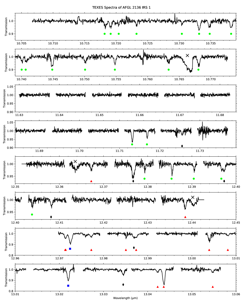
Figure 3: Shown here are the mid infrared spectra of AFGL 2136 IRS 1 in select regions from 10.7-13.1 $\mu$m obtained with TEXES. The various symbols beneath the spectra mark absorption features due to NH₃ (green circles), H₂O (black diamonds), HCN (blue squares), and C₂H₂ (red triangles). Black crosses above broad features indicate that these are likely artifacts caused by poor matching of the target and telluric standard spectra at the edge of echelle orders.

One final step was required for processing the CRIRES observations since data were acquired at the same settings on multiple nights. Where multiple spectra cover the same wavelength range, they were combined using a weighted average (weighted by 1/$\sigma^{2}$, where $\sigma$ is the standard deviation of the line-free continuum in each spectrum). In this way, all of the individual CRIRES spectra were combined to form a single normalized spectrum. This spectrum and the normalized spectra resulting from the EXES and TEXES observations are presented in Figures 1–3.

4 Results & Analysis

It is apparent from Figures 1–3 that AFGL 2136 IRS 1 displays a wealth of absorption features. In addition to the H₂O absorption we identify features due to H${}_{2}^{18}$O ($\nu_{2}=1$–0 band), HF ($\nu=1$–0 band), CO ($\nu=2$–0 band), HCN ($\nu_{2}=1$–0 band), C₂H₂ ($\nu_{5}=1$–0 band), and NH₃ ($\nu_{2}=1$–0 band). We also find three broad emission features due to the Pfund series of atomic hydrogen, and a set of unidentified absorption features near 2.49 $\mu$m that are also observed toward the massive protostar AFGL 4176 (Karska et al., in preparation).

4.1 H₂O Absorption

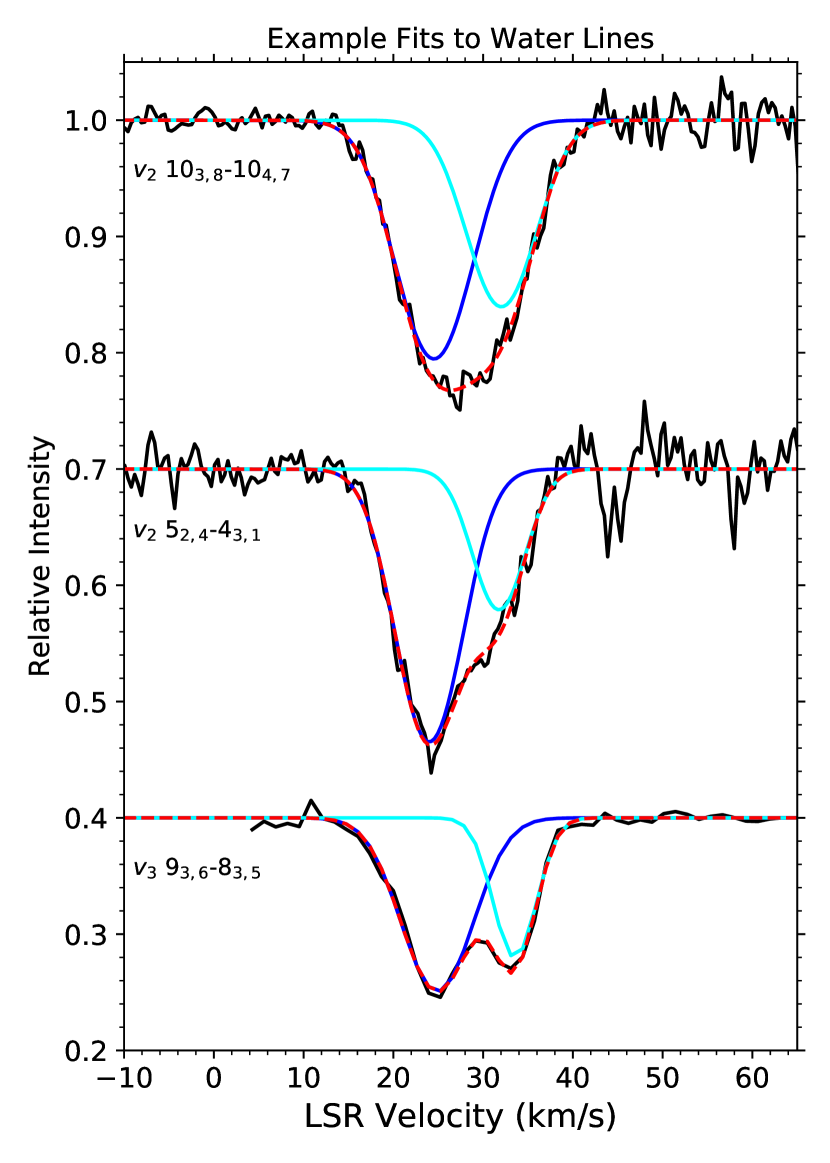
Figure 4: Two-component gaussian fits to H₂O absorption lines are shown here. The blue and cyan curves mark the components at about 25 km s^-1 and 33 km s^-1, while the red dashed curve is the sum of both components.

More than 100 absorption features are present in these spectra, including many that are blends due to absorption from multiple transitions. Using the temperature and total H₂O column density inferred from our previous study of this source (Indriolo et al., 2013a) and assuming local thermodynamic equilibrium (LTE), we predicted the strength of all H₂O absorption lines covered by our data. By comparing these predictions to the observed spectra we identified absorption features that are due to individual transitions of H₂O (i.e., are not blends of multiple H₂O transitions or blends of an H₂O transition and that of another species). Starting with some of the stronger $\nu_{3}$ band features, we fit absorption lines (in optical depth space) with a sum of two gaussian components to determine average fit parameters. The line center velocities ($v_{cent}$) and line widths ($\sigma_{v}$) determined from these fits were then used as initial guesses for fitting the other unblended absorption features. During the fitting procedure these free parameters were restricted to values similar to the initial guesses. The line center velocities of both components were constrained to remain within $\pm 4$ km s^-1 of the initial guesses (20–28 km s^-1 and 28–36 km s^-1 for components 1 and 2, respectively), and line widths for both components were constrained to the range 1 km s${}^{-1}\leq\sigma_{v}\leq 6$ km s^-1. In this manner, all of the unblended H₂O absorption features were fit with line profiles that are the sum of two gaussian functions in optical depth. Some example fits are shown in Figure 4. Note that it is unlikely that the two components utilized in the fit correspond to two distinct physical components, as will be discussed in Section 5.4.

Using the best-fit parameters we determined an integrated optical depth ($\int\tau dv$) for each component. Uncertainties were computed using the covariance matrix returned by scipy.optimize.curve_fit. The column density in the lower rotational state associated with the transition ($N_{l}$) was calculated via the standard equation for optically thin absorption:

$$N_{l}=\frac{8\pi}{A_{ul}\lambda^{3}}\frac{g_{l}}{g_{u}}\int\tau dv,$$ (1)

where $\lambda$ is the transition wavelength, $A_{ul}$ is the transition spontaneous emission coefficient, and $g_{l}$ and $g_{u}$ are the statistical weights of the lower and upper states, respectively, including nuclear spin degeneracy (i.e., $g=(2J+1)(2I+1)$, where $I=0$ for para-H₂O and $I=1$ for ortho-H₂O). Transition data were taken from the HITRAN database (Rothman et al., 2013). Total column densities in each rotational state are taken to be the sum of the column densities determined from the two components, and the resulting $\ln(N_{l}/g_{l})$ are presented in Table 2.

4.2 H₂O Rotation Diagrams

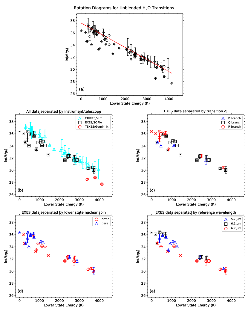
Figure 5: These rotation diagrams for H₂O in AFGL 2136 IRS 1 are color coded by different discrete properties of the transitions and rotational states from which column densities were determined. Note that for EXES data the uncertainties are generally smaller than the markers. The red dashed line in panel (a) is the best-fit line for the CRIRES data alone, and corresponds to the temperature and H₂O column density reported in Table 3.

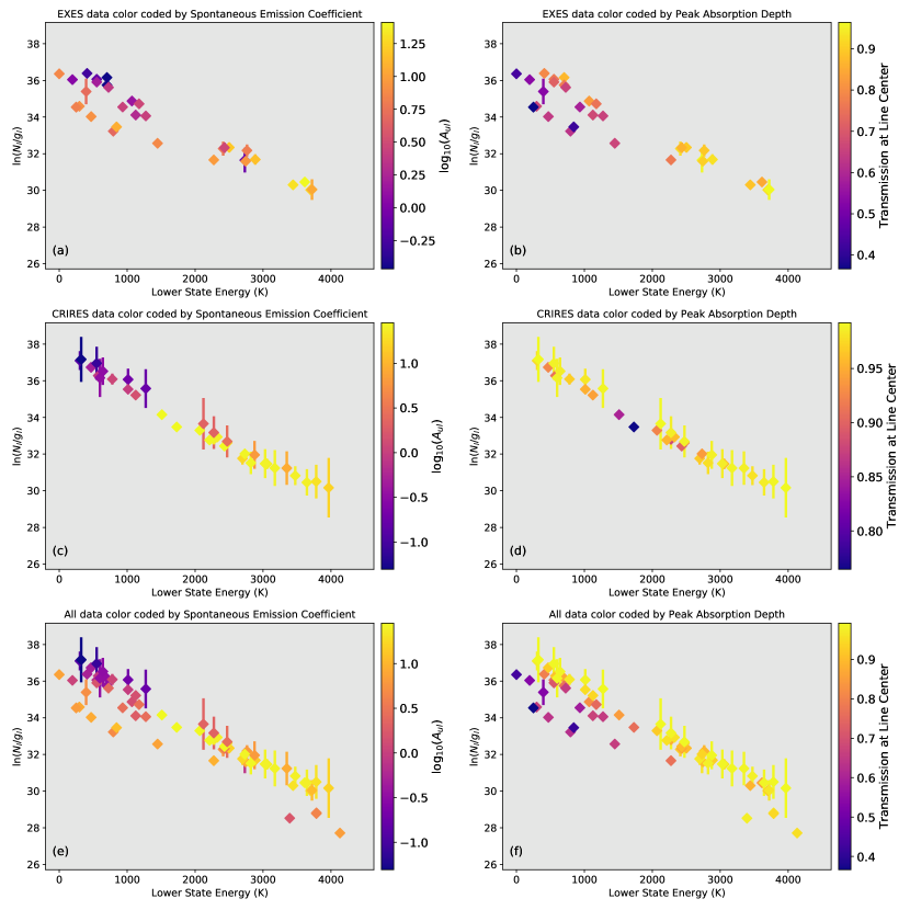
Figure 6: These rotation diagrams for H₂O in AFGL 2136 IRS 1 are color coded by spontaneous emission coefficient of the transition from which a column density was determined (panels (a), (c), and (e)) and by the maximum depth of the absorption feature from which a column density was determined (panels (b), (d), and (f)). Panels (a) and (b) show only EXES data, panels (c) and (d) show only CRIRES data, and panels (e) and (f) show all data.

Column densities determined for individual rotational states are used to construct a rotation (Boltzmann) diagram for H₂O (Figures 5 and 6). For gas in LTE at a single temperature ($T$) the points should form a straight line with a slope equal to $-T^{-1}$. While this is reasonably true in Figure 5 panel (a), the large scatter in $\ln{(N_{l}/g_{l})}$ is not explained by this simple isothermal absorbing slab model. In particular, the column densities of a significant number of states fall below the best fit straight line for the majority of levels by as much as a factor of ten. To investigate this issue, we explore whether or not certain lower-state and/or transition characteristics correlate with states that appear to be “under-populated”.

In Figure 5 the points on the rotation diagram are distinguished by different discrete properties of the lower rotational state or the observed transition. Panel (b) has points separated by the instrument with which each transition was observed. It is clear that points from different instruments behave in different ways, but it is unlikely that this is an effect of the different instruments themselves (see Section 5.3). The SOFIA/EXES data show significant scatter, so that sub-set of data can be used to further investigate the observed behavior. Panel (c) shows EXES data separated by the change in the rotational quantum number of the transition ($\Delta J=1$, 0, and $-$1 are the $R$, $Q$, and $P$ branches, respectively). There does not appear to be any significant correlation between $\Delta J$ and $\ln{(N_{l}/g_{l})}$. Panel (d) shows EXES data separated by the nuclear spin (the ortho and para nuclear spin configurations correspond to $K_{a}+K_{c}$ being odd and even, respectively) of the lower state, and again, there is no correlation with $\ln{(N_{l}/g_{l})}$. Although not presented here, the CRIRES data similarly show no correlation between $\ln{(N_{l}/g_{l})}$ and nuclear spin configuration, and indicate an ortho-to-para ratio of 3:1. Panel (e) separates the EXES data by the three different observed wavelength ranges. While there is some distinction between the different points, “under-populated” states are not unique to any given wavelength range, and above about 2500 K there is no discrepancy between any of the points. As such, the scatter does not appear to be caused by the three separate EXES observations at different wavelengths.

In Figure 6 the points on the rotation diagram are distinguished by color scales that are used to indicate the spontaneous emission coefficient of the transition from which each column density was determined (panels (a), (c), and (e)), and the transmission level at the point of deepest absorption within each absorption feature from which column densities were determined (panels (b), (d), and (f)). For EXES observations the “under-populated” states have column densities determined from stronger absorption features (panel (b)), and for states with $E_{l}<2500$ K the scatter in $\ln{(N_{l}/g_{l})}$ is correlated with $A_{ul}$, with column densities in “under-populated” states derived from transitions with larger spontaneous emission coefficients (panel (a)). Hints of these same trends are possibly present in the CRIRES observations shown in panels (c) and (d), although they are within the range of uncertainties for many of the inferred column densities. Panels (e) and (f) show the same plots for all data. It is clear from panel (f) that there is a correlation between the depth of absorption features and how far the column densities derived from those features deviate from their expected values. Only the TEXES data points deviate from this pattern. A more in-depth discussion about what may cause these behaviors follows in Section 5.3.

Despite the scatter present in the rotation diagrams, a linear fit to the data points can still be used to infer the gas temperature and total H₂O column density. It is clear from Figure 5 though that this fit will change based on the subset of data points being used, as is demonstrated by the results presented in Table 3. Given the large scatter in the EXES data and the relatively linear, self-consistent behavior of the CRIRES data, we adopt the results obtained from the CRIRES data alone: $N({\rm H_{2}O})=(8.25\pm 0.95)\times 10^{18}$ cm^-2 and $T=502\pm 12$ K. A fit using the 6.7 $\mu$m EXES data alone results in a temperature that is 1.6 times higher than, and a total H₂O column density that is 8 times lower than the adopted values. This implies that results derived from different and/or limited wavelength ranges should be viewed with caution (e.g., Indriolo et al., 2015), and that future observations should be planned with care to minimize such effects. Table 3 also shows that a fit to all of the EXES data does not agree with our adopted values. As the upper envelope of EXES data points is consistent with the CRIRES data though (panel (b) of Figure 5), it should still be possible to infer reasonably accurate values of $T$ and $N({\rm H_{2}O})$ in sources where only EXES observations have been made by restricting the fit to a subset of the EXES data points. For example, limiting the fit to EXES data where column densities were derived from weak absorption features (line center transmission $>75$%; $\tau_{0}<0.29$) produces results in better agreement with the CRIRES results (see Table 3). In future cases where scatter similar to that shown here is seen in rotation diagrams, we recommend restricting the linear fit to only include state-specific column densities determined from weak absorption lines when deriving total column densities and rotation temperatures.

4.3 Other species

4.3.1 Absorption Lines

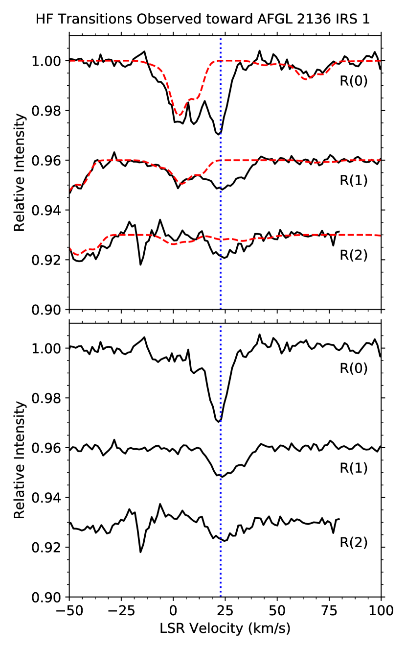
Figure 7: Shown here are absorption lines of HF observed toward AFGL 2136 IRS 1. The blue vertical dotted line marks the systemic velocity of 22.8 km s^-1 (as measured from molecular emission lines; van der Tak et al., 2000b). In the top panel solid black lines are the observed spectra and dashed red curves are simulated absorption spectra of H₂O. The bottom panels shows the ratio of the observed and simulated spectra to more clearly present the HF line profiles. The narrow feature near $-17$ km s^-1 in the $R(2)$ spectrum is due to poor removal of a telluric absorption line.

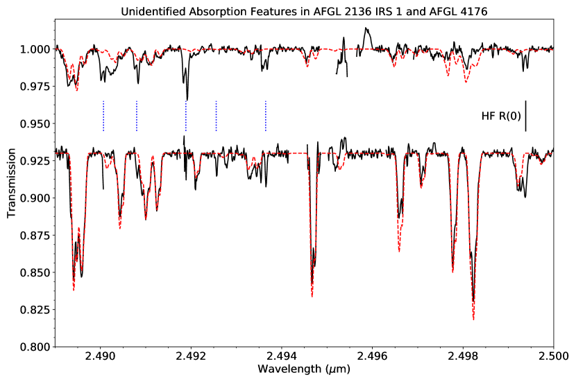
Figure 8: Spectra of AFGL 2136 IRS 1 (bottom) and AFGL 4176 (top; Karska et al., in preparation) highlighting unidentified absorption features are shown here. Dotted blue lines mark the unidentified absorption features at 2.490070 $\mu$m, 2.490800 $\mu$m, 2.491885 $\mu$m, 2.492555 $\mu$m, and 2.493645 $\mu$m. Both spectra have been shifted in wavelength so that absorption lines appear at their rest wavelengths. Red dashed curves are model H₂O absorption spectra generated as discussed in Section 4.3.1. The HF $R(0)$ line is marked with a solid black line to demonstrate that its line shape is similar to that of the unidentified features (single peak in AFGL 2136 IRS 1 and double peak in AFGL 4176). This similarity suggests that the species responsible for these absorption lines resides in the cooler foreground gas, not the warm gas where H₂O absorption arises.

A variety of molecular absorption features are observed toward AFGL 2136 IRS 1. Some of these species (NH₃, HCN, and C₂H₂) dominate the absorption features at 10–13 $\mu$m, but at 2.5 $\mu$m H₂O is the most prevalent absorber. Despite the fact that a uniform absorbing slab model cannot successfully predict the H₂O absorption from 2–13 $\mu$m, such a model is still useful in analyzing the CRIRES observations to search for features caused by other species. Using the average gaussian parameters inferred from the two-component fit described above ($v_{1}=24.8$ km s^-1, $\sigma_{1}=4.16$ km s^-1, $v_{2}=33.7$ km s^-1, $\sigma_{2}=2.92$ km s^-1), adopting the total $N({\rm H_{2}O})$ and $T$ inferred from only the CRIRES data, and assuming that the component at 24.8 km s^-1 contains 70% of the material, we generate a synthetic H₂O absorption spectrum (see Figures 1, 7, and 8). The top panel of Figure 7 shows the synthetic H₂O spectrum at the wavelengths of the $v=1$–0 $R(0)$, $R(1)$, and $R(2)$ transitions of HF, demonstrating that all three HF transitions are detected in absorption. The bottom panel of Figure 7 shows the AFGL 2136 IRS 1 spectrum after division by the synthetic H₂O spectrum, effectively showing the absorption due to only HF. By fitting the HF absorption features after division by the synthetic H₂O spectrum, we find individual state column densities of $N(0)=(3.1\pm 0.8)\times 10^{14}$ cm^-2, $N(1)=(2.6\pm 1.3)\times 10^{14}$ cm^-2, and $N(2)=(1.6\pm 1.4)\times 10^{14}$ cm^-2, consistent with our previous observations (Indriolo et al., 2013b). The $R(0)$ line shows a different profile from the $R(1)$ and $R(2)$ lines, suggesting that the excited states may be tracing a warmer gas component than the ground state. While less prominent than the HF features, absorption lines due to the $P(34)$–$P(37)$ transitions of the $v=2$–0 band of CO are also detected (Figure 1). These features are too weak to perform meaningful fits, but their depths are in agreement with predictions based on the temperature and column density of the warm CO component reported by Goto et al. (2019).

Figure 8 shows portions of the spectra of AFGL 2136 IRS 1 and AFGL 4176 (Karska et al., in preparation) where the synthetic H₂O spectrum fails to reproduce five different absorption features. To determine the rest wavelengths of these features we matched the line profiles for the unidentified lines with that of the HF $R(0)$ line in the case of AFGL 4176, and that of the H${}_{3}^{+}$ $R(1,1)^{u}$ line (from Goto et al., 2019) in the case of AFGL 2136 IRS 1. The resulting rest wavelengths are 2.490070 $\mu$m, 2.490800 $\mu$m, 2.491885 $\mu$m, 2.492555 $\mu$m, and 2.493645 $\mu$m, with uncertainties of about $5\times 10^{-6}$ $\mu$m. We were unable to identify the one or more species that causes these absorption features, although based on the line profiles the carrier must reside in the cooler foreground component, and not the warm gas that gives rise to H₂O absorption.

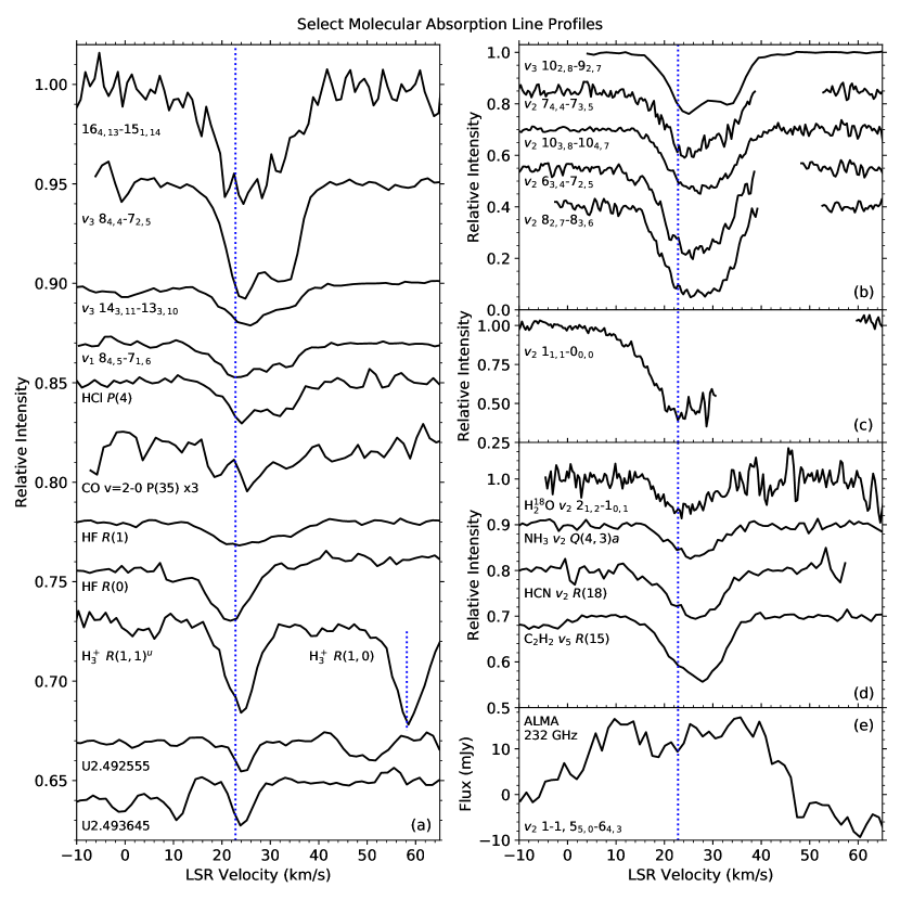
Figure 9: A selection of absorption line profiles from H₂O and other species observed within our spectra is shown here. Note that instrumental line profiles have not been removed. Labels that do not include a molecule name indicate features due to H₂O. Panel (a) shows weak ($\lesssim 5$% deep) absorption features due to a pure rotational H₂O line, lines from the $\nu_{1}$ and $\nu_{3}$ vibrational bands of H₂O at 2.7 $\mu$m, HCl (Goto et al., 2013), CO (scaled up by a factor of 3), HF (after division by the model H₂O spectrum), H${}_{3}^{+}$ (Goto et al., 2019), and two unidentified lines. Panel (b) shows one H₂O transition from the $\nu_{3}$ band, and several from the $\nu_{2}$ band. Panel (c) shows the $\nu_{2}$ $1_{1,1}$–$0_{0,0}$ transition of H₂O, which probes the ground rotational state. Panel (d) shows absorption from H${}_{2}^{18}$O, NH₃, HCN, and C₂H₂. Panel (e) shows the H₂O $\nu_{2}=1-1$ $5_{5,0}$–$6_{4,3}$ line at 232.687 GHz in emission observed with ALMA (extracted from a rectangular region defined by ($\alpha_{2000}$,$\delta_{2000}$)=($18^{h}22^{m}26^{s}.38857$, $-13^{\circ}30\arcmin 12\farcs 0226$) and ($18^{h}22^{m}26^{s}.38372$, $-13^{\circ}30\arcmin 11\farcs 9216$) from the publicly available data cube provided by Maud et al., 2019). Inspection of the data cube suggests that line emission ranges from about 3 km s^-1 to 45 km s^-1. Vertical dashed lines mark the systemic velocity at 22.8 km s^-1. In general, there appear to be three categories of line profiles: H₂O, HCl, HF $R(1)$, CO $P(35)$, NH₃, HCN, and C₂H₂ show broad, potentially 2-component features that are red-shifted from systemic; H${}_{3}^{+}$ and the unidentified lines show narrow features that are slightly red-shifted from systemic (with the caveat that rest wavelengths for the unidentified features were determined in part by profile matching to the H${}_{3}^{+}$ line); HF $R(0)$ shows one component that is at the systemic velocity, and agrees with low-$J$ CO $v=2$–0 absorption profiles (Goto et al., 2019). H₂O absorption from the ground rotational state extends to lower velocities compared to other transitions, and may also be probing cooler foreground material.

Example line profiles from all detected species are presented in Figure 9. A variety of strong H₂O absorption lines are shown in panel (b), while weak H₂O lines are in the top half of panel (a). Panel (c) shows absorption out of the H₂O ground rotational state. Panel (d) shows absorption due to ro-vibrational transitions of H${}_{2}^{18}$O, NH₃, HCN, and C₂H₂, all of which have line profiles that are consistent with those observed for H₂O in the mid-IR. The bottom half of panel (a) shows absorption due to HCl (Goto et al., 2013), CO, H${}_{3}^{+}$ (Goto et al., 2019), and HF, as well as two unidentified lines. The HCl $P(4)$ absorption profile matches that of H₂O, while the profiles of H${}_{3}^{+}$ and the unidentified lines do not. HF is more complicated as the $R(0)$ line shows one component at the systemic velocity, while the $R(1)$ and $R(2)$ line profiles resemble the H₂O absorption. This suggests that the excited HF is tracing the same material as the H₂O, while the ground state HF is tracing a cooler foreground component that has been observed at $T\approx 60$ K in the low $J$ transitions of the $v=2$–0 band of CO (Goto et al., 2019). The NH₃, HCN, and C₂H₂ line profiles also suggest that these species reside in the warm gas component that gives rise to H₂O absorption. For comparison with the absorption lines, panel (e) shows the H₂O $\nu_{2}=1-1$ $5_{5,0}$–$6_{4,3}$ line at 232.687 GHz observed in emission by ALMA (extracted from the publicly available data cube provided by Maud et al., 2019).

4.3.2 Emission Lines

In addition to the plethora of absorption features seen in the AFGL 2136 IRS 1 spectra, a few broad emission features are also present. These can be seen in Figure 1, and are due to the $n=19$–5 and 18–5 transitions of the Pfund series of atomic H. The 17–5 transition was also seen in emission but suffered heavy interference from telluric H₂O lines and so was removed from the spectrum during the normalization process. A zoom in on the 19–5 and 18–5 emission features is shown in Figure 10. The 19–5 line is centered at 31 km s^-1 with a FWHM of 96 km s^-1, while the 18–5 line is centered at 39 km s^-1 with a FWHM of 127 km s^-1. Note, however, that our normalization and baseline removal procedures were optimized for the analysis of narrow absorption features, not broad emission features, so these values are highly uncertain.

4.4 Multi-Epoch Observations

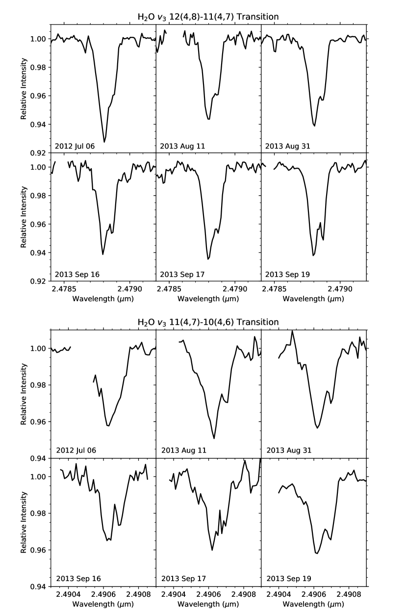
Figure 11: Different panels show the absorption profiles of the H₂O $\nu_{3}$ 12_4,8–11_4,7 transition (top) and H₂O $\nu_{3}$ 11_4,7–10_4,6 transition (bottom) from the six different nights when our VLT/CRIRES observations executed. All spectra have been shifted into the LSR frame.

The CRIRES spectrum presented in Figure 1 is the average spectrum from observations taken on six different nights (see Table 1). Some unblended H₂O absorption lines were covered at all six epochs, so we can check for variability in the absorption profiles. Figure 11 shows the $\nu_{3}$ 12_4,8–11_4,7 (top panel) and $\nu_{3}$ 11_4,7–10_4,6 (bottom panel) transitions of H₂O from each individual night of observations. In the top panel all of the observations from 2013 (39 days maximum separation) agree within the noise level, but the observation from 2012 suggests a deeper absorption feature with a less well-defined shoulder component toward longer wavelengths. In the bottom panel all of the observations, including that from 2012, agree with each other within the noise level. However, this line in 2012 again lacks the well-defined shoulder that is present in all of the 2013 observations. It is difficult to draw any firm conclusions from these spectra. While the TEXES and EXES observations provide additional epochs in 2014 and 2016, respectively, due to the different instruments utilized, aperture sizes, and transitions observed any such comparison would be highly uncertain. Still, the general agreement of the H₂O line profiles from the different telescopes in Figure 9 is indicative of no significant changes over a 4 year timescale.

5 Discussion

The AFGL 2136 region has been extensively observed over the past few decades at several wavelengths, angular resolutions, and spectral resolutions, with each new study contributing information in the quest to understand its physical and chemical structure. While part of the story certainly unfolds at larger spatial scales—bipolar molecular outflows (100″; Kastner et al., 1994; Maud et al., 2015), near-IR reflection nebula (10″; Kastner et al., 1992; Murakawa et al., 2008), ice absorption in the cold envelope (e.g., Keane et al., 2001b; Dartois et al., 2002; Gibb et al., 2004)—here we focus the discussion primarily on the smaller spatial scales immediately surrounding IRS 1.

5.1 Warm and Hot Molecular Gas

The first indication of hot molecular gas near AFGL 2136 IRS 1 came from observations of the $v=1$–0 band of ¹³CO and $v=2$–1 band of ¹²CO in absorption (Mitchell et al., 1990). A hot component was determined to have $N(^{13}{\rm CO})=(2.5\pm 0.7)\times 10^{17}$ cm^-2 and $T=580^{+60}_{-50}$ K, containing about twice as much material as a cold component, and was hypothesized to arise in gas close to the central protostar. Recent observations of the $v=2$–0 band of ¹²CO confirm this picture, finding $N(^{12}{\rm CO})=(2.8\pm 0.4)\times 10^{19}$ cm^-2 and $T=534\pm 80$ K (Goto et al., 2019). The absorption line profiles for ¹²CO $v=2$–0 transitions out of highly excited levels (e.g., $R$(21) and $R$(23)) are consistent with those we find for H₂O, suggesting that both species are tracing the same component.

Observations with the Infrared Space Observatory Short Wavelength Spectrometer (ISO-SWS) have also revealed absorption from a variety of gas phase molecules tracing warm gas, including CO₂, SO₂, H₂O, HCN, and C₂H₂. While the large wavelength coverage of ISO-SWS enables the observation and analysis of entire ro-vibrational bands, the resolution does not allow for the study of kinematics, individual line profiles, and state-specific column densities. Additionally, the determination of total column densities and excitation temperatures requires the use of assumed line widths. Analyses of molecular absorption bands observed toward AFGL 2136 IRS 1 by ISO-SWS have resulted in a range of excitation temperatures: $T_{ex}({\rm CO}_{2})=300\pm 100$ K (Boonman et al., 2003); $T_{ex}({\rm SO}_{2})=350_{-50}^{+100}$ K (Keane et al., 2001a); $T_{ex}({\rm H_{2}O})=500_{-150}^{+250}$ K (Boonman & van Dishoeck, 2003); $T_{ex}({\rm HCN})=600_{-50}^{+75}$ K (Lahuis & van Dishoeck, 2000); $T_{ex}({\rm C_{2}H_{2}})=800_{-100}^{+150}$ K (Lahuis & van Dishoeck, 2000). The cause of the large scatter in excitation temperatures is unclear, and it is difficult to evaluate if this scatter is real, or if the excitation temperatures agree within uncertainties. Still, it is reasonable to associate these absorption features with the same (or a similar) gas component as that probed by the hot CO. Without kinematic information though, it was not possible to confirm this hypothesis from the ISO-SWS observations alone.

In the past several years, observations of AFGL 2136 IRS 1 in the near-to-mid infrared have been made at much higher spectral resolution ($\sim 3$ km s^-1). Our previous observations of H₂O with CRIRES confirmed the high excitation temperature ($T_{ex}({\rm H_{2}O})=506\pm 25$ K), but indicated a total H₂O column density about seven times larger than that determined from ISO-SWS ($N({\rm H_{2}O})=(1.02\pm 0.02)\times 10^{19}$ cm^-2 vs. $N({\rm H_{2}O})=(1.5\pm 0.6)\times 10^{18}$ cm^-2; Indriolo et al., 2013a; Boonman & van Dishoeck, 2003). The resolved H₂O line profiles were in reasonable agreement with the hot CO component from Mitchell et al. (1990), but without access to the CO data it was still not possible to directly compare the two species. Now, with our new H₂O observations and the recent CO $v=2$–0 observations presented by Goto et al. (2019), we can definitively say that both species show the same absorption line profiles, and very likely reside in the same physical component. This same component may also give rise to the NH₃, C₂H₂, and HCN absorption—as suggested by Figure 9—and this topic will be further addressed by Barr et al. (in preparation). Although HCl shows a similar absorption profile to H₂O and CO, the excitation temperature inferred from the observed transitions is significantly lower: $T_{ex}({\rm HCl})\approx 250$ K (Goto et al., 2013). This is reminiscent of the scatter in the ISO-SWS results (if real), and potentially suggests that either: (a) the species do not trace exactly the same material, but perhaps different layers of the same kinematic structure; or (b) excitation temperatures derived from individual molecules are not good indicators of the kinetic temperature of the gas since level populations may be influenced by radiative processes.

ALMA observations of AFGL 2136 IRS 1 have recently revealed emission from the hot molecular gas component as well. The H₂O $\nu_{2}=1$–1, $5_{5,0}$-$6_{4,3}$ transition at 232.687 GHz, which originates from a state $E_{u}=3461.9$ K above ground, is observed tracing a compact disk ($\sim 93$ mas diameter) in Keplerian rotation about a central object with mass $45\pm 10$ M_☉ (Maud et al., 2019). The velocity centroid along the disk minor axis is in agreement with the line-center velocity of the stronger component found from our gaussian fitting procedure (24.8 km s^-1), suggesting that the H₂O absorption we observe in the IR may arise in the disk now imaged at sub-mm wavelengths. Compact SiO emission ($J=5$–4; 217.105 GHz; $E_{u}=31.3$ K) has also been observed toward AFGL 2136 IRS 1 with ALMA. A portion of the SiO emission shows similar kinematics as H₂O and likely traces the disk (Maud et al., 2019), but emission near the systemic velocity is more spatially extended and hypothesized to arise in a rotating disk wind (Maud et al., 2018). Perhaps different conditions in these two components are responsible for the different rotation temperatures inferred from various molecules.

5.2 Hot Ionized Gas

Even more compact than the disk around AFGL 2136 IRS 1 is a region producing emission in transitions indicative of ionized gas. The H30$\alpha$ recombination line is spatially unresolved with ALMA’s 20 mas beam, but there is a hint of rotation in the same sense as the H₂O emission (Maud et al., 2019). It has a very broad line profile that is centered at 22.1 km s^-1, with $FWHM\sim 81.9\pm 1.7$ km s^-1 (Maud et al., 2018). This is likely the same region that gives rise to the H Pfund $n=19$–5 and 18–5 emission lines shown in our Figure 10 as the electrons cascade down toward the ground electronic state following recombination. Similar emission features from the $n=21$–6 and 19–6 transitions of the Humphreys series of atomic H near 3.6 $\mu$m have also been observed toward AFGL 2136 IRS 1 (M. Goto, private communication), and the hydrogen Br$\gamma$ ($n=7$–4) line has been observed with $FWHM_{\rm Br\gamma}\approx 133$ km s^-1 (Murakawa et al., 2013). Hydrogen Br$\gamma$ emission in massive protostars has previously been interpreted as emission from an outflowing stellar wind or disk wind (e.g., Malbet et al., 2007; Murakawa et al., 2013), although the spatially unresolved H30$\alpha$ emission requires the emitting region to be much smaller than the circumstellar disk.

5.3 Understanding the H₂O Spectrum

The optimal use of spectroscopy in studying massive protostars entails understanding what underlying characteristics cause the observed absorption and emission features. While the use of a simple isothermal absorbing slab model that is removed from and fully covering a background source can be instructive, its assumptions and limitations—many of which are described in Lacy (2013)—prevent such a model from re-producing observed spectra. To re-iterate some of those points: (1) the central protostar will produce a temperature gradient in the surrounding gas and dust; (2) the absorbing gas can be mixed with the warm dust that serves as the “background” continuum; (3) molecules both emit and absorb light. Here, we discuss how these and other effects can influence the observed spectra.

A covering fraction of less than one (i.e., clumpy absorbing material that does not cover the entire background source) is a scenario that has previously been invoked to explain observed IR absorption spectra (e.g., Knez, 2006; Knez et al., 2009; Barentine & Lacy, 2012; Indriolo et al., 2015). In this case, saturated absorption lines will have a depth equal to the covering fraction, and all lines will appear weaker than expected, since total absorption corresponds to a relative intensity larger than zero. While some absorption features are about 4 times weaker than expected assuming the H₂O column density and excitation temperature inferred from CRIRES data alone (e.g., $\nu_{2}$ 2_1,1-3_2,2 at 6.723374 $\mu$m), others are about as strong as expected (e.g., $\nu_{2}=2-1$ 7_1,6-7_2,5 at 6.726109 $\mu$m). Since covering fraction would affect all line depths equally, this explanation does not seem feasible. Even if the absorbing material does not fully cover the background source, the deepest absorption feature in the spectrum (H₂O $\nu_{2}$ 3_2,1-3_1,2 at 6.075447 $\mu$m) reaches a transmission level of about 0.3, so a minimum covering fraction of 70% is required for the EXES observations.

One of the obvious differences amongst our spectra is the instruments used in performing the observations. In particular the CRIRES, EXES, and TEXES observations were made using slits with different widths and lengths (widths of 0$\farcs$2, 1$\farcs$84, and 0$\farcs$54, respectively), so light from slightly different regions is being observed in each case. The larger apertures could probe regions with different conditions than probed by the narrowest (CRIRES) slit from which we infer column density and temperature. Extended continuum emission (assuming the absorbing gas is not extended) or extended line emission could fill in the absorption features. The extended continuum explanation is equivalent to a covering fraction argument though, and so is ruled out. Extended line emission would have to be limited to only those transitions that are weaker than expected, but should also manifest as emission lines if a spectrum is extracted slightly off of the continuum peak. No H₂O line emission is seen when we extract a spectrum slightly off source, so this scenario seems unlikely as well.

Previous observations of molecular absorption and emission lines in the mid-IR have demonstrated different behaviors of transitions within a ro-vibrational band. The $\nu_{2}$ band of H₂O has shown some lines in emission and others in absorption (Gonzalez-Alfonso et al., 1998; González-Alfonso & Cernicharo, 1999), as has the $\nu_{2}$ band of NH₃ (Barentine & Lacy, 2012). In both of these studies though, there is a pattern that the $R$-branch lines appear in absorption, while the $P$-branch lines appear in emission, explained by the relative importance of the radiative pathways that populate and de-populate the vibrationally excited rotational levels. If this mechanism were responsible for the large scatter in the rotation diagrams—not to the point of causing emission, but just enough to fill in some of the absorption—then there should be a discrepancy in the column densities inferred from $R$-branch and $P$-branch transitions. Panel (c) of Figure 5 shows no correlation between “under-populated” states and transition $\Delta J$ though, so this emission mechanism is also unable to explain the observed spectra.

The parameter that shows the clearest correlation with a state being “under-populated” is the depth of the absorption feature from which the state-specific column density was derived (Figure 6, panels (b), (d), and (f)). Excepting the absorption features observed with TEXES, deeper absorption lines tend to result in more “under-populated” states. This can be explained by a scenario where the absorbing gas is well mixed with the warm dust that serves as a “background” source of continuum emission. Blackbody continuum emission predominantly comes from the $\tau\approx 1$ “surface”, so any observed line absorption only comes from gas above that surface. The depth of the $\tau\approx 1$ “surface” depends on the dust opacity (and associated absorption coefficient, $\kappa_{\nu}$), which is dependent on wavelength (Draine, 2003) and on the distribution of dust grain sizes (e.g. Agurto-Gangas et al., 2019), so the layers of gas probed by observations at 2 $\mu$m, 6 $\mu$m, and 13 $\mu$m may be different. Because the absorption coefficient is also affected by line processes, $\kappa_{\nu}$ is larger at the wavelengths of transitions with larger spontaneous emission coefficients. This means that the physical depth where $\tau\approx 1$ is shallower for stronger lines than for weaker lines, such that there is a smaller column of gas in front of the “background” source. In this case, it is not that any levels are under-populated with respect to LTE, just that they appear that way from a simple absorbing slab analysis since different transitions probe to different depths within the absorbing gas.

The above scenario requires that the absorbing gas and source of continuum emission be well mixed. Mid-IR (8–13 $\mu$m) interferometric observations of AFGL 2136 IRS 1 are suggestive of an elongated structure that has a size and orientation reasonably consistent with the recently reported sub-mm disk (de Wit et al., 2011; Boley et al., 2013; Maud et al., 2019). This indicates that the continuum emission at wavelengths longer than about 8 $\mu$m likely arises in the disk, and so it is reasonable to assume that the gas is mixed with the emitting dust for the TEXES observations. For silicate dust at the dust sublimation temperature ($T\sim 1300$ K; Kobayashi et al., 2011) the blackbody spectrum peaks at about 2.2 $\mu$m, so the dust disk is expected to be bright in the near infrared as well. Radiative transfer models of near infrared interferometric observations of another massive protostar suggest that the dominant continuum emission source at 2.2 $\mu$m in that system is a circumstellar disk (Kraus et al., 2010, IRAS 13481$-$6124), so thermal emission from the warm dust disk may be the dominant continuum source in all of our observations from 2.5–13 $\mu$m (Beltrán & de Wit, 2016).

Of the effects discussed above, the mixing of warm dust and absorbing gas seems to be the most likely explanation for the observed H₂O absorption spectrum. ALMA observations have shown that the dust disk and gas disk have roughly the same physical extent (Maud et al., 2019), and it is plausible that the warm dust in the disk dominates the continuum at all observed wavelengths. The H₂O absorption line profiles, however, are not consistent with expectations in a scenario where the entire disk is responsible for continuum emission and molecular absorption. To better understand what may cause this discrepancy, a more detailed investigation of the line profiles is required.

5.4 Line Profiles

Given the gas temperature inferred for the AFGL 2136 IRS 1 disk, line profiles are expected to be dominated entirely by orbital motions rather than thermal broadening. As such, information about gas kinematics is contained within the absorption and emission line profiles. H₂O absorption lines observed with CRIRES show two distinct absorption peaks while those observed with EXES and TEXES do not, but in all cases lines are well described by two gaussian components. The robustness of individual gaussian fit parameters is difficult to assess, as in many cases intensity can be traded between the two components without adversely affecting the overall fit, so it is not particularly instructive to consider the properties of the two fit components separately. Indeed, the single temperature required to describe the rotation diagram for CRIRES data and the relatively constant intensity ratio between the two components in the CRIRES data suggest that all of the absorption arises in a single physical component.

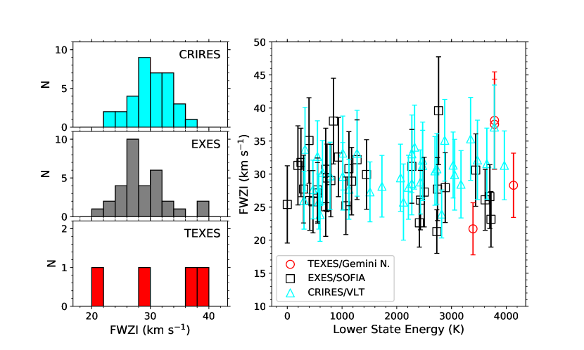
Figure 12: The distribution of FWZI line widths ($|v_{2}-v_{1}|+3\sigma_{1}+3\sigma_{2}$) is plotted for H₂O absorption features observed with the three different instruments in the panels on the left hand side. There is a marginal decrease in FWZI from the CRIRES data to the EXES data. The right hand panel shows FWZI as a function of lower state energy for all unblended H₂O lines. No correlation is seen between the two parameters. FWZI line width uncertainties are dominated by the fits to the line wings.

Absorption lines arising in circumstellar disks have previously been observed toward FU Ori type objects (young, low mass stars experiencing luminosity bursts due to enhanced accretion; Hartmann & Kenyon, 1996, and references therein). The fact that the lines appear in absorption rather than emission is indicative of a temperature inversion in the disk, where heating due to accretion causes the disk midplane to be warmer than the surface. Two properties observed in absorption lines toward FU Ori type objects are that: (1) many absorption features are double-peaked; and (2) the width of absorption features tends to decrease with increasing wavelength. The double-peaked nature of the lines is explained by a disk in Keplerian rotation, with the two absorption peaks caused by the blueshifted and redshifted sides of the disk. While we do see double-peaked absorption lines toward AFGL 2136 IRS 1, the underlying explanation is not quite the same, as will be discussed below. The anticorrelation between linewidth and wavelength is explained by the temperature in the disk decreasing with increased distance from the central source. Continuum emission at shorter wavelengths preferentially arises in warmer material at small radii where orbital velocities are large, so the absorbing gas produces broad features. At longer wavelengths the continuum emission arises from larger radii where orbital velocities are smaller, hence narrower absorption lines. An analysis of the distribution of full-width-at-zero-intensity (FWZI) line widths (defined as $|v_{2}-v_{1}|+3\sigma_{1}+3\sigma_{2}$) shows a marginal decrease (1.5 km s^-1 in the mean value) between H₂O lines at 2.5 $\mu$m and 5.7–6.7 $\mu$m (Figure 12). As FWZI line widths are broad (30 km s^-1 on average) and instrumental profiles have not been removed from the spectra, it is difficult to determine if this shift is real.

The line profile for the 232 GHz H₂O emission extracted over the full extent of the disk is shown in Figure 9 panel (e). Inspection of the data cube channel by channel suggests that the flux at $v\lesssim 3$ km s^-1 is an artifact of the image processing, and that the H₂O emission from the disk extends from about 3 km s^-1 to about 45 km s^-1. Emission at these extreme velocities arises from the innermost portions of the disk along the major axis, and the velocity centroid along the disk minor axis is halfway between these two extremes at 24 km s^-1. The line profile has two emission peaks, with one each arising from the redshifted and blueshifted halves of the disk. All of these features are consistent with a disk in Keplerian rotation, as reported by Maud et al. (2019).

H₂O absorption profiles—and those of other molecules—clearly do not show the same characteristics as the 232 GHz H₂O emission. The strongest H₂O absorption occurs at about 25 km s^-1 with a second weaker component at about 33 km s^-1, and absorption extends from about 12 to 40 km s^-1. The narrower (with respect to emission), asymmetric line profiles seen in absorption suggest that if the H₂O absorption arises within the disk, it is not tracing the entire disk. In particular, the absence of absorption at the extreme velocities, and the lack of an absorption component at $v\leq 24$ km s^-1 indicate that H₂O absorption probes neither the innermost portion of the disk along the major axis, nor the blueshifted half of the disk. An examination of Figure 1b in Maud et al. (2019) provides a potential explanation for this observed behavior. There, the 1.3 mm continuum emission shows clumpy structure within the disk after an assumed point source caused by free-free emission has been removed. The strongest continuum peaks within the disk are located along the minor axis, where $v\approx 24$ km s^-1 is expected, and near the outer edge of the redshifted side, where $v\approx 33$ km s^-1 is expected. These velocities are in good agreement with the two absorption components that are observed. If the clumpy structure seen in the 1.3 mm continuum emission is indicative of the 2–13 $\mu$m continuum structure, this could explain the molecular absorption profiles seen in the near-to-mid-IR.

As the ALMA observations were performed on 2017 Oct 10, the disk sub-structure at the time of the IR observations would have been oriented slightly differently. Material at the inner and outer disk radii of 30 AU and 120 AU has orbital periods of about 24 yr and 196 yr, respectively (assuming a central mass of 45 $M_{\sun}$), and would move by at most 18 mas and 9 mas in the plane of the sky over the 5.3 yr between our first CRIRES observation and the ALMA observations given a distance of 2.2 kpc. This suggests that the majority of the substructure identified in the ALMA observations was in a reasonably similar orientation at the time when the IR observations were performed.

Finally, we note that there is no evidence for a high velocity wind component in absorption toward AFGL 2136 IRS 1. CO absorption lines observed toward some massive protostars show broad blueshifted wings, extending over $-100$ km s^-1 from the systemic velocity (e.g., van der Tak et al., 1999). Neither the H₂O nor the CO (Mitchell et al., 1990; Smith et al., 2014; Goto et al., 2019) absorption lines observed toward AFGL 2136 IRS 1 show such a broad component. Most likely this is simply due to the orientation of the disk and outflow system, such that wind and outflow components are not probed by the pencil beam line of sight toward the continuum source.

5.5 Conditions in the AFGL 2136 IRS 1 Disk

In our previous study of H₂O absorption observed with CRIRES toward AFGL 2136 IRS 1 we used a statistical equilibrium code to infer conditions within the absorbing gas (Indriolo et al., 2013a). The code modeled the excitation of the lowest 120 rotational states of ortho- and para-H₂O to determine the expected level populations under a variety of physical conditions. In this code the effects of radiative trapping are treated using an escape probability method, and collisional rate coefficients between H₂O and H₂ were taken from Daniel et al. (2011), and were extrapolated to higher energy states for which calculations are unavailable using an artificial neural network method (Neufeld, 2010). Radiative pumping effects in both ro-vibrational and rotational transitions due to the infrared continuum emission from AFGL 2136 IRS 1 were also included, assuming the spectral energy distribution implied by a fit to the data obtained by Murakawa et al. (2008, the TO model plotted in their Figure 7). This analysis demonstrated that the observed state specific column densities could be explained by purely collisional excitation, purely radiative excitation, or some contribution from both mechanisms between these two extremes. In the collisionally dominated case the gas is at high density and temperature ($n({\rm H_{2}})\gtrsim 5\times 10^{9}$ cm^-3; $T=506\pm 25$ K). In the radiatively dominated case a $T=700$ K blackbody subtends 2$\pi$ sr (i.e., half of the sky) as seen by the gas, the gas temperature is unconstrained, and the density must be $n({\rm H_{2}})\lesssim 10^{6}$ cm^-3. Note that these two scenarios are limiting cases, and that some combination of collisional and radiative excitation is also viable, in which case the inferred constraints are relaxed (e.g., if excitation is primarily through collisions, but also due in some part to radiation, then the lower limit on the density will decrease compared to that in the purely collisional case).

We repeated this same statistical equilibrium analysis on the H₂O column densities presented here in Table 2, but were unable to find a model capable of simultaneously reproducing all values. This failure can be attributed to the large scatter in the rotation diagrams caused by different transitions probing different depths within the disk, as discussed above. Limiting the analysis to only the CRIRES data produces the same results as in Indriolo et al. (2013a) that are summarized above, so we do not present the entire analysis anew in this paper.

Given the limits on gas density and the measured H₂O column density, we can place constraints on the size of the region that contains H₂O. The relative abundance of H₂O with respect to H₂ in warm gas is expected to be about 10^-4 (van Dishoeck et al., 2013, and references therein), so the radiatively dominated case suggests an upper limit of $n({\rm H_{2}O})\lesssim 100$ cm^-3. With $N({\rm H_{2}O})=8.25\times 10^{18}$ cm^-2, this requires a minimum path length of $l\gtrsim 8.25\times 10^{16}$ cm, or about 5500 AU. The collisionally dominated case requires $n({\rm H_{2}O})\gtrsim 5\times 10^{5}$ cm^-3, corresponding to a maximum path length of $l\lesssim 1.65\times 10^{13}$ cm, or about 1.1 AU. It is clear that the path length over which absorption occurs in the radiatively dominated case is incompatible with the $r\sim 120$ AU size scales of the AFGL 2136 IRS 1 disk. The path length in the collisionally dominated case however, is consistent with the picture where the observed H₂O absorption is coming from the upper layers of the disk. That said, the fact that the H₂O resides within the disk means that blackbody radiation from the dust disk must have some influence on the excitation of H₂O, so the absorbing layer can be thicker than that determined for the scenario where only collisions are considered.

Although Figure 11 shows the possibility of marginal variability in H₂O absorption line profiles, the similarity of the line profiles in the CRIRES, EXES, and TEXES data shown in Figure 9 suggests no significant changes in the absorbing material over 4 year time scales. This is further evidence against a scenario where the background continuum source and absorbing gas are separated (e.g., gas in the disk absorbing light from the central protostar), because the absorbing material in a pencil beam toward the central object will change as it orbits. The time between our first CRIRES observation and last EXES observation was 1357 days. Over this time period, gas at radii of 30 AU and 120 AU in Keplerian rotation about a 45 $M_{\sun}$ star would move 28.6 AU and 14.3 AU along their respective orbits. The disk material would have to be uniform over these size scales in order for the absorption profile to remain nearly constant in a pencil beam toward the central object over 4 years. If portions of the disk itself serve as the background continuum source though, then the material above the $\tau\approx 1$ “surface” will be probed by absorption spectroscopy, regardless of where the material is in its orbit. Time variability in line profiles is still expected in this case though, as the 1.3 mm continuum emission shows substructure (Maud et al., 2019). As regions of brighter continuum emission orbit the central object, the absorption from the gas associated with these regions will shift in velocity.

5.6 H₂O Isotopologues

In our observations, absorption due to both the H${}_{2}^{16}$O and H${}_{2}^{18}$O isotopologues of H₂O is detected. With only two unblended H${}_{2}^{18}$O lines observed we cannot estimate the total column density of that isotopologue, but we can compare state-specific column densities. Transitions probing the $J_{K_{a},K_{c}}=3_{1,2}$ state of both H${}_{2}^{16}$O and H${}_{2}^{18}$O are observed in our spectrum, providing column densities of $N({\rm H_{2}^{16}O}|3_{1,2})=(21.1\pm 0.84)\times 10^{15}$ cm^-2 and $N({\rm H_{2}^{18}O}|3_{1,2})=(2.23\pm 0.86)\times 10^{15}$ cm^-2 (see Table 2). This state-specific analysis results in ${\rm H_{2}^{16}O/H_{2}^{18}O}=9.5$, much smaller than the oxygen isotopic ratio found in the solar system (¹⁶O/¹⁸O $\approx 500$; Asplund et al., 2009, and references therein). However, the H${}_{2}^{16}$O $\nu_{2}=1-0$ $3_{2,1}$-$3_{1,2}$ transition is one of the strongest absorption features in our spectrum, suggesting that it traces a much smaller region than the optically thin H${}_{2}^{18}$O $\nu_{2}=1-0$ $3_{2,1}$-$3_{1,2}$ transition. Rather than representing the real isotopic ratio then, this is another indicator of the optical depth effects discussed above. The best-fit temperature and H${}_{2}^{16}$O column density can be used to estimate the state-specific column densities for H${}_{2}^{16}$O corresponding to the two observed H${}_{2}^{18}$O transitions for use in determining isotopic ratios. Using this method we find $N({\rm H_{2}^{16}O}|1_{0,1})=1.79\times 10^{17}$ cm^-2 and $N({\rm H_{2}^{16}O}|3_{1,2})=2.71\times 10^{17}$ cm^-2. Together with the measured H${}_{2}^{18}$O state-specific column densities, these values give ${\rm H_{2}^{16}O/H_{2}^{18}O}\approx 206$ and ${\rm H_{2}^{16}O/H_{2}^{18}O}\approx 121$. Although still below the solar system isotopic ratio, these are well within the wide range of values found in other stellar atmospheres (Hinkle et al., 2016).

6 Summary

We have observed H₂O absorption toward the massive protostar AFGL 2136 IRS 1 at high ($\sim 3$ km s^-1) spectral resolution in wavelength intervals near 2.5 $\mu$m, 6 $\mu$m, and 13 $\mu$m. H₂O absorption line profiles are consistent with those from other molecules that trace a hot gas component (e.g., NH₃, HCN, C₂H₂, HCl, highly excited CO), and do not match the profiles of sub-mm molecular emission lines that arise in the cooler, more extended envelope. Analysis of a rotation diagram constructed from state-specific column densities indicates an H₂O column density of $N({\rm H_{2}O})=(8.25\pm 0.95)\times 10^{18}$ cm^-2 at a temperature of $T=502\pm 12$ K. It is clear, however, that an isothermal absorbing slab model in LTE does not adequately describe the relative intensities of all observed H₂O absorption lines. The most likely explanation for the H₂O line depths is that the absorbing gas is well mixed with the warm dust that serves as the “background” continuum source at 2.5–13 $\mu$m. Because the $\tau\approx 1$ “surface” in this model is wavelength dependent and moves to shallower depths for stronger lines, the stronger lines are effectively probing a smaller region than the weaker lines. This is why the absorption features that should be the deepest are much shallower than expected, and also why fitting a line to only the upper envelope of points in the rotation diagram provides the best estimate of the total H₂O column density, although with the caveat that this still only provides the column density down to the $\tau\approx 1$ “surface” for weak lines.

Recent ALMA observations of AFGL 2136 IRS 1 have revealed a compact ($93\times 71$ mas) disk that shows Keplerian rotation in the H₂O $\nu_{2}=1$–1, 5_5,0-6_4,3 transition at 232.687 GHz. The velocity at which the strongest H₂O absorption occurs in the infrared coincides with the H₂O emission velocity centroid along the disk minor axis. We conclude that the H₂O absorption observed in the infrared—as well as the absorption caused by other molecules that (1) have similar absorption profiles, and (2) indicate high rotational temperatures—arises within this circumstellar disk. Additionally, the warm dust in this disk is the dominant source of continuum emission at our observed wavelengths. Molecular absorption in the IR can thus serve as a powerful probe of accretion disks around massive protostars.

The authors thank the anonymous referee for providing suggestions to improve the quality of our paper. N.I. thanks M. Goto for providing VLT/CRIRES spectra of AFGL 2136 IRS 1 at 3.6 $\mu$m so that HCl and H${}_{3}^{+}$ line profiles could be included within this paper. M.J.R. and EXES observations are supported by NASA cooperative agreement NNX13AI85A. A.K. acknowledges support from the First TEAM grant of the Foundation for Polish Science No. POIR.04.04.00-00-5D21/18-00 and the Polish National Science Center grant 2016/21/D/ST9/01098. Support for this work was provided by the Polish National Agency for Academic Exchange through the project InterAPS.

Based on observations collected at the European Southern Observatory under ESO programmes 089.C-0321(B) and 091.C-0335(A). Based on observations made with the NASA/DLR Stratospheric Observatory for Infrared Astronomy (SOFIA). SOFIA is jointly operated by the Universities Space Research Association, Inc. (USRA), under NASA contract NNA17BF53C, and the Deutsches SOFIA Institut (DSI) under DLR contract 50 OK 0901 to the University of Stuttgart. [Financial support for this work was provided by NASA through award #04-0120 issued by USRA.] Based on observations obtained at the Gemini Observatory, which is operated by the Association of Universities for Research in Astronomy, Inc., under a cooperative agreement with the NSF on behalf of the Gemini partnership: the National Science Foundation (United States), National Research Council (Canada), CONICYT (Chile), Ministerio de Ciencia, Tecnología e Innovación Productiva (Argentina), Ministério da Ciência, Tecnologia e Inovação (Brazil), and Korea Astronomy and Space Science Institute (Republic of Korea). Observations were obtained as part of program GN-2014B-Q-103.

Table 1: Log of Observations of AFGL 2136 IRS 1 and Objects used as Telluric standards

Target	Telescope	Instrument	Reference Wavelength	Date	Altitude	Slit Width	Exposure Time
			(nm / cm-1)		(m)	(arcsec)	(s)
AFGL 2136 IRS 1	VLT UT1	CRIRES	2502.8	2012 Jul 6	2635	0.2	3960
AFGL 2136 IRS 1	VLT UT1	CRIRES	2502.8	2013 Aug 11	2635	0.2	2340
AFGL 2136 IRS 1	VLT UT1	CRIRES	2480.0	2013 Aug 31	2635	0.2	2340
AFGL 2136 IRS 1	VLT UT1	CRIRES	2502.8	2013 Sep 16	2635	0.2	2160
AFGL 2136 IRS 1	VLT UT1	CRIRES	2480.0	2013 Sep 17	2635	0.2	2340
AFGL 2136 IRS 1	VLT UT1	CRIRES	2502.8	2013 Sep 19	2635	0.2	2340
HR 6378	VLT UT1	CRIRES	2502.8	2013 Aug 11	2635	0.2	300
HR 6378	VLT UT1	CRIRES	2480.0	2013 Aug 31	2635	0.2	840
HR 6378	VLT UT1	CRIRES	2502.8	2013 Sep 16	2635	0.2	300
HR 6378	VLT UT1	CRIRES	2480.0	2013 Sep 17	2635	0.2	300
HR 6378	VLT UT1	CRIRES	2502.8	2013 Sep 19	2635	0.2	300
AFGL 2136 IRS 1	SOFIA	EXES	1485.90	2016 Mar 24	13410	1.84	650
AFGL 2136 IRS 1	SOFIA	EXES	1640.15	2016 Mar 24	13102	1.84	720
AFGL 2136 IRS 1	SOFIA	EXES	1748.25	2016 Mar 24	13100	1.84	480
$\alpha$ CMa	SOFIA	EXES	1485.90	2016 Mar 18	12814	1.84	884
$\alpha$ CMa	SOFIA	EXES	1640.15	2016 Mar 24	11593	1.84	840
$\alpha$ CMa	SOFIA	EXES	1747.58	2016 Mar 18	11280	1.84	416
AFGL 2136 IRS 1	Gemini N.	TEXES	931.5	2014 Aug 11	4213	0.54	712
AFGL 2136 IRS 1	Gemini N.	TEXES	856.0	2014 Aug 14	4213	0.54	210
AFGL 2136 IRS 1	Gemini N.	TEXES	806.5	2014 Aug 17	4213	0.54	396
AFGL 2136 IRS 1	Gemini N.	TEXES	768.5	2014 Aug 18	4213	0.54	406
16 Psyche	Gemini N.	TEXES	931.5	2014 Aug 11	4213	0.54	2372
16 Psyche	Gemini N.	TEXES	856.0	2014 Aug 14	4213	0.54	648
16 Psyche	Gemini N.	TEXES	806.5	2014 Aug 17	4213	0.54	1626
16 Psyche	Gemini N.	TEXES	768.5	2014 Aug 18	4213	0.54	1406

Table 2: Results from Unblended H₂O Absorption Lines

$v^{\prime}-v^{\prime\prime}$	$J_{K_{a},K_{c}}^{\prime}-J_{K_{a},K_{c}}^{\prime\prime}$	Wavelength	$E_{l}$	$A_{ul}$	$g_{u}$	$g_{l}$	$\int\tau dv$	ln$(N_{l}/g_{l})$	$N_{\rm meas}/N_{\rm pred}$
		($\mu$m)	(K)	(s-1)			(km s-1)
$\nu_{3}=1-0$	$8_{3,5}$-$7_{1,6}$	2.446108	1013.2	0.979	51	45	0.79$\pm$0.15	35.53$\pm$0.19	0.96
$\nu_{3}=1-0$	$5_{5,1}$-$4_{3,2}$	2.447276	550.4	0.082	33	27	0.18$\pm$0.16	36.95$\pm$0.90	1.58
$\nu_{3}=1-0$	$7_{2,5}$-$6_{0,6}$	2.450228	642.7	0.321	15	13	0.20$\pm$0.15	36.52$\pm$0.75	1.23
$\nu_{3}=1-0$	$8_{4,4}$-$7_{2,5}$	2.451345	1125.7	1.480	51	45	0.87$\pm$0.15	35.22$\pm$0.17	0.88
$\nu_{3}=1-0$	$14_{5,9}$-$13_{5,8}$	2.453230	3783.0	20.510	87	81	0.19$\pm$0.17	30.50$\pm$0.92	1.56
$\nu_{3}=1-0$	$6_{4,3}$-$5_{2,4}$	2.454677	598.8	0.339	13	11	0.13$\pm$0.14	36.16$\pm$1.04	0.78
$\nu_{3}=1-0$	$14_{4,10}$-$13_{4,9}$	2.461582	3645.6	25.020	87	81	0.22$\pm$0.16	30.46$\pm$0.72	1.13
$\nu_{1}=1-0$	$8_{4,5}$-$7_{1,6}$	2.467807	1013.2	0.194	51	45	0.27$\pm$0.16	36.07$\pm$0.58	1.64
$\nu_{1}=1-0$	$12_{6,7}$-$11_{5,6}$	2.468616	2876.1	6.393	75	69	0.22$\pm$0.17	31.96$\pm$0.76	1.10
$\nu_{3}=1-0$	$13_{4,9}$-$12_{4,8}$	2.468911	3173.4	25.930	27	25	0.15$\pm$0.15	31.24$\pm$0.98	0.97
$\nu_{3}=1-0$	$7_{3,4}$-$6_{1,5}$	2.472935	781.1	1.202	15	13	0.51$\pm$0.15	36.09$\pm$0.30	1.05
$\nu_{1}=1-0$	$11_{6,5}$-$10_{5,6}$	2.473202	2472.8	2.726	69	63	0.18$\pm$0.16	32.69$\pm$0.87	1.02
$\nu_{3}=1-0$	$14_{6,8}$-$13_{6,7}$	2.473837	3965.9	16.270	87	81	0.11$\pm$0.17	30.16$\pm$1.62	1.60
$\nu_{1}=1-0$	$11_{5,6}$-$10_{4,7}$	2.475249	2275.2	2.115	69	63	0.22$\pm$0.20	33.17$\pm$0.89	1.12
$\nu_{3}=1-0$	$14_{3,11}$-$13_{3,10}$	2.477481	3474.2	24.950	87	81	0.32$\pm$0.16	30.82$\pm$0.51	1.16
$\nu_{3}=1-0$	$12_{4,8}$-$11_{4,7}$	2.478598	2732.2	26.170	75	69	0.95$\pm$0.15	32.01$\pm$0.16	0.87
$\nu_{1}=1-0$	$9_{3,6}$-$8_{2,7}$	2.479768	1274.2	0.170	57	51	0.17$\pm$0.17	35.57$\pm$1.05	1.68
$\nu_{1}=1-0$	$5_{4,1}$-$4_{1,4}$	2.480526	323.5	0.049	33	27	0.14$\pm$0.17	37.17$\pm$1.23	1.24
$\nu_{3}=1-0$	$13_{3,10}$-$12_{3,9}$	2.483376	3029.9	25.500	27	25	0.20$\pm$0.15	31.48$\pm$0.79	0.92
$\nu_{3}=1-0$	$6_{2,4}$-$5_{0,5}$	2.484255	468.1	0.494	39	33	1.05$\pm$0.14	36.73$\pm$0.14	1.08
$\nu_{1}=1-0$	$10_{6,4}$-$9_{5,5}$	2.486180	2122.2	2.179	21	19	0.12$\pm$0.16	33.66$\pm$1.40	1.34
$\nu_{2}=2-0$	$15_{3,12}$-$14_{2,13}$	2.488795	3349.3	8.645	93	87	0.18$\pm$0.17	31.23$\pm$0.91	1.37
$\nu_{3}=1-0$	$11_{4,7}$-$10_{4,6}$	2.490420	2325.7	24.690	23	21	0.70$\pm$0.17	32.93$\pm$0.24	0.97
$\nu_{3}=1-0$	$13_{4,10}$-$12_{4,9}$	2.491232	3057.3	24.010	81	75	0.55$\pm$0.16	31.46$\pm$0.28	0.96
$\nu_{3}=1-0$	$4_{4,0}$-$3_{2,1}$	2.492091	305.2	0.127	27	21	0.27$\pm$0.14	37.10$\pm$0.51	1.12
$\nu_{3}=1-0$	$6_{3,3}$-$5_{1,4}$	2.494654	574.7	0.922	39	33	1.27$\pm$0.14	36.28$\pm$0.11	0.85
$\nu_{3}=1-0$	$11_{3,8}$-$10_{3,7}$	2.496575	2213.0	27.470	23	21	0.67$\pm$0.15	32.77$\pm$0.22	0.66
$\nu_{3}=1-0$	$13_{2,11}$-$12_{2,10}$	2.497063	2820.3	27.190	27	25	0.22$\pm$0.13	31.52$\pm$0.61	0.63
$\nu_{3}=1-0$	$12_{2,10}$-$11_{2,9}$	2.504591	2432.5	27.810	75	69	1.60$\pm$0.15	32.44$\pm$0.09	0.73
$\nu_{3}=1-0$	$11_{4,8}$-$10_{4,7}$	2.511261	2275.2	23.560	69	63	1.81$\pm$0.15	32.80$\pm$0.08	0.77
$\nu_{3}=1-0$	$11_{2,9}$-$10_{2,8}$	2.512036	2068.9	27.820	23	21	1.17$\pm$0.15	33.30$\pm$0.13	0.84
$\nu_{3}=1-0$	$11_{5,7}$-$10_{5,6}$	2.512708	2472.8	19.930	69	63	1.27$\pm$0.16	32.62$\pm$0.12	0.95
$\nu_{3}=1-0$	$9_{3,6}$-$8_{3,5}$	2.517545	1510.9	28.400	19	17	2.33$\pm$0.14	34.15$\pm$0.06	0.65
$\nu_{3}=1-0$	$11_{6,6}$-$10_{6,5}$	2.518460	2697.7	17.010	69	63	0.46$\pm$0.15	31.76$\pm$0.33	0.63
$\nu_{3}=1-0$	$10_{2,8}$-$9_{2,7}$	2.519438	1729.3	28.430	63	57	3.95$\pm$0.13	33.48$\pm$0.03	0.51
$\nu_{2}=1-0$	$7_{4,4}$-$7_{3,5}$	5.705113	1175.0	2.981	15	15	3.97$\pm$0.50	34.72$\pm$0.12	0.59
$\nu_{2}=1-0$	$8_{1,8}$-$7_{0,7}$	5.709642	843.5	11.840	51	45	15.25$\pm$1.18	33.46$\pm$0.08	0.09
$\nu_{2}=1-0$	$11_{3,8}$-$11_{2,9}$	5.713061	2432.5	3.049	69	69	1.71$\pm$0.47	32.33$\pm$0.27	0.66
$\nu_{2}=1-0$	$6_{4,3}$-$6_{3,4}$	5.716237	933.7	2.772	39	39	8.11$\pm$0.52	34.55$\pm$0.06	0.31
$\nu_{2}=1-0$	$5_{2,4}$-$4_{1,3}$	5.718679	396.4	5.157	11	9	9.94$\pm$6.93	35.39$\pm$0.70	0.24
$\nu_{2}=2-1$	$10_{1,10}$-$9_{0,9}$	5.720222	3614.6	25.810	63	57	2.04$\pm$0.47	30.46$\pm$0.23	1.06
$\nu_{2}=1-0$	$5_{4,2}$-$5_{3,3}$	5.721717	725.1	2.390	11	11	5.76$\pm$0.50	35.62$\pm$0.09	0.59
$\nu_{2}=1-0$	$8_{1,7}$-$8_{0,8}$	5.726424	1070.5	1.397	17	17	2.48$\pm$0.46	34.87$\pm$0.19	0.56
$\nu_{2}=1-0$	$4_{4,0}$-$4_{3,1}$	5.728111	552.3	1.617	9	9	4.28$\pm$0.48	35.91$\pm$0.11	0.56
$\nu_{2}=1-0$	$8_{3,6}$-$8_{2,7}$	5.731998	1274.2	2.692	51	51	6.38$\pm$0.53	34.06$\pm$0.08	0.37
$\nu_{2}=1-0$	$3_{2,1}$-$3_{1,2}$	6.075447	249.4	6.715	21	21	12.62$\pm$0.50	34.54$\pm$0.04	0.08
$\nu_{2}=2-1$	$5_{1,4}$-$5_{0,5}$	6.080180	2763.5	6.406	33	33	1.78$\pm$0.58	32.18$\pm$0.33	1.09
$\nu_{2}=1-0$	$5_{3,2}$-$4_{4,1}$	6.088700	702.3	0.351	33	27	3.48$\pm$0.40	35.75$\pm$0.12	0.64
$\nu_{2}=1-0$	$5_{2,4}$-$4_{3,1}$	6.096408	552.3	0.733	11	9	3.33$\pm$0.34	36.06$\pm$0.10	0.65
$\nu_{2}=2-1$	$2_{2,1}$-$2_{1,2}$	6.100969	2412.9	5.916	15	15	0.84$\pm$0.32	32.28$\pm$0.38	0.60
$\nu_{2}=1-0$	$5_{3,3}$-$4_{4,0}$	6.103987	702.3	0.343	11	9	1.72$\pm$0.38	36.16$\pm$0.22	0.96
$\nu_{2}=1-0$	$4_{2,2}$-$3_{3,1}$	6.106193	410.4	0.529	9	7	2.73$\pm$0.31	36.38$\pm$0.11	0.67
$\nu_{2}=1-0$	$3_{1,2}$-$2_{2,1}$	6.106826	194.1	1.123	21	15	9.60$\pm$0.72	36.04$\pm$0.08	0.31
$\nu_{2}=2-1$	$4_{0,4}$-$3_{1,3}$	6.113164	2502.7	15.800	9	7	1.44$\pm$0.36	32.34$\pm$0.25	0.77
$\nu_{2}=1-0$	$1_{1,1}$-$0_{0,0}$	6.116331	0.0	7.457	3	1	12.55$\pm$0.66	36.36$\pm$0.05	0.29
$\nu_{2}=1-0$	$10_{3,8}$-$10_{4,7}$	6.705153	2275.2	9.459	63	63	4.03$\pm$0.27	31.66$\pm$0.07	0.25
$\nu_{2}=1-0$	$4_{0,4}$-$5_{1,5}$	6.707693	469.9	8.449	9	11	5.46$\pm$0.24	34.03$\pm$0.04	0.07
$\nu_{2}=2-1$	$4_{2,2}$-$4_{3,1}$	6.711310	2886.1	14.320	9	9	0.89$\pm$0.25	31.69$\pm$0.28	0.85
$\nu_{2}=1-0$	$6_{1,6}$-$6_{2,5}$	6.712122	795.5	4.825	39	39	6.10$\pm$0.33	33.23$\pm$0.05	0.06
$\nu_{2}=1-0$	$6_{3,4}$-$7_{2,5}$	6.714553	1125.7	1.928	39	45	5.91$\pm$0.26	34.11$\pm$0.04	0.29
$\nu_{2}=1-0$	$8_{2,7}$-$8_{3,6}$	6.715692	1447.6	7.602	51	51	6.52$\pm$0.25	32.57$\pm$0.04	0.12
$\nu_{2}=1-0$	$13_{4,10}$-$13_{5,9}$	6.722649	3721.4	11.270	27	27	0.41$\pm$0.23	30.04$\pm$0.56	0.87
$\nu_{2}=1-0$	$2_{1,1}$-$3_{2,2}$	6.723374	296.8	8.223	5	7	5.22$\pm$0.58	34.59$\pm$0.11	0.09
$\nu_{2}=2-1$	$7_{1,6}$-$7_{2,5}$	6.726109	3442.4	20.140	45	45	1.59$\pm$0.27	30.30$\pm$0.17	0.65
$\nu_{2}=2-1$	$3_{2,1}$-$3_{3,0}$	6.733401	2744.6	9.039	21	21	1.21$\pm$0.26	31.59$\pm$0.21	0.59
$\nu_{2}=1-0$	$10_{5,6}$-$11_{4,7}$	6.737377	2732.2	0.804	63	69	0.34$\pm$0.23	31.65$\pm$0.67	0.60
$\nu_{2}=2-1$	$7_{3,4}$-$7_{4,3}$	6.753573	3700.7	17.650	45	45	1.07$\pm$0.26	30.03$\pm$0.24	0.82
	$16_{3,14}$-$15_{0,15}$	11.724550	3393.1	1.682	99	93	0.26$\pm$0.03	28.52$\pm$0.13	0.10
	$16_{4,13}$-$15_{1,14}$	12.375657	3785.8	4.211	99	93	0.99$\pm$0.05	28.78$\pm$0.05	0.28
	$16_{3,13}$-$15_{2,14}$	12.407046	3785.8	4.217	33	31	0.35$\pm$0.06	28.82$\pm$0.17	0.29
	$16_{5,12}$-$15_{2,13}$	13.033327	4132.6	6.761	99	93	0.64$\pm$0.06	27.71$\pm$0.09	0.19
H${}_{2}^{18}$O
$\nu_{2}=1-0$	$2_{1,2}$-$1_{0,1}$	6.074293	34.2	6.533	15	9	0.84$\pm$0.34	32.20$\pm$0.40	…
$\nu_{2}=1-0$	$3_{2,1}$-$3_{1,2}$	6.103487	248.7	6.404	21	21	1.29$\pm$0.50	32.30$\pm$0.39	…

Note. — Transition properties for all unblended lines fit during our analysis are shown here. Integrated optical depths ($\int\tau dv$) are over the entire absorption feature (i.e., the sum of the two components). Individual state column densities assuming optically thin absorption are presented as $\ln(N_{l}/g_{l})$. These values should be considered with extreme caution given the discussion presented in this paper. The last column gives the ratio between the measured and predicted state-specific column densities. Predicted column densities assume an isothermal absorbing slab in LTE with the temperature and total H₂O column density determined from CRIRES observations alone (see Table 3). Smaller values correspond to more “under-populated” states.

Table 3: Rotation Diagram Analysis Comparison

Data Sub-Sample	Temperature	$N({\rm H_{2}O})$
	(K)	(1018 cm-2)
All Data 2.44–13.1 $\mu$m	$545\pm 24$	$4.13\pm 0.80$
CRIRES 2.44–2.52 $\mu$m	$502\pm 12$	$8.25\pm 0.95$
EXES 5.7–6.76 $\mu$m	$628\pm 44$	$2.48\pm 0.60$
EXES 5.7–5.74 $\mu$m	$627\pm 81$	$2.94\pm 1.15$
EXES 6.07–6.12 $\mu$m	$626\pm 85$	$3.85\pm 1.48$
EXES 6.7–6.76 $\mu$m	$812\pm 63$	$1.05\pm 0.28$
EXES 5.7–6.76 $\mu$m, $\tau_{0}<0.29$	$519\pm 19$	$5.13\pm 0.94$

Note. — Temperatures and total H₂O column densities are inferred from linear fits to rotation diagrams made from different sub-sets of individual state column densities determined from unblended absorption lines.

References

- Agurto-Gangas et al. (2019) Agurto-Gangas, C., Pineda, J. E., Szűcs, L., et al. 2019, A&A, 623, A147, doi: 10.1051/0004-6361/201833666
- Asplund et al. (2009) Asplund, M., Grevesse, N., Sauval, A. J., & Scott, P. 2009, ARA&A, 47, 481, doi: 10.1146/annurev.astro.46.060407.145222
- Astropy Collaboration et al. (2013) Astropy Collaboration, Robitaille, T. P., Tollerud, E. J., et al. 2013, A&A, 558, A33, doi: 10.1051/0004-6361/201322068
- Barentine & Lacy (2012) Barentine, J. C., & Lacy, J. H. 2012, ApJ, 757, 111, doi: 10.1088/0004-637X/757/2/111
- Beltrán & de Wit (2016) Beltrán, M. T., & de Wit, W. J. 2016, A&A Rev., 24, 6, doi: 10.1007/s00159-015-0089-z
- Boley et al. (2013) Boley, P. A., Linz, H., van Boekel, R., et al. 2013, A&A, 558, A24, doi: 10.1051/0004-6361/201321539
- Boonman & van Dishoeck (2003) Boonman, A. M. S., & van Dishoeck, E. F. 2003, A&A, 403, 1003, doi: 10.1051/0004-6361:20030364
- Boonman et al. (2003) Boonman, A. M. S., van Dishoeck, E. F., Lahuis, F., & Doty, S. D. 2003, A&A, 399, 1063, doi: 10.1051/0004-6361:20021868
- Clarke et al. (2015) Clarke, M., Vacca, W. D., & Shuping, R. Y. 2015, in Astronomical Society of the Pacific Conference Series, Vol. 495, Astronomical Data Analysis Software an Systems XXIV (ADASS XXIV), ed. A. R. Taylor & E. Rosolowsky, 355
- Cushing et al. (2004) Cushing, M. C., Vacca, W. D., & Rayner, J. T. 2004, PASP, 116, 362, doi: 10.1086/382907
- Daniel et al. (2011) Daniel, F., Dubernet, M.-L., & Grosjean, A. 2011, A&A, 536, A76, doi: 10.1051/0004-6361/201118049
- Dartois et al. (2002) Dartois, E., d’Hendecourt, L., Thi, W., Pontoppidan, K. M., & van Dishoeck, E. F. 2002, A&A, 394, 1057, doi: 10.1051/0004-6361:20021228
- de Wit et al. (2011) de Wit, W. J., Hoare, M. G., Oudmaijer, R. D., et al. 2011, A&A, 526, L5, doi: 10.1051/0004-6361/201016062
- Draine (2003) Draine, B. T. 2003, ARA&A, 41, 241, doi: 10.1146/annurev.astro.41.011802.094840
- Gibb et al. (2004) Gibb, E. L., Whittet, D. C. B., Boogert, A. C. A., & Tielens, A. G. G. M. 2004, ApJS, 151, 35, doi: 10.1086/381182
- González-Alfonso & Cernicharo (1999) González-Alfonso, E., & Cernicharo, J. 1999, ApJ, 525, 845, doi: 10.1086/307909
- Gonzalez-Alfonso et al. (1998) Gonzalez-Alfonso, E., Cernicharo, J., van Dishoeck, E. F., Wright, C. M., & Heras, A. 1998, ApJ, 502, L169, doi: 10.1086/311503
- Goto et al. (2019) Goto, M., Geballe, T. R., Harju, J., et al. 2019, A&A, 632, A29, doi: 10.1051/0004-6361/201936119
- Goto et al. (2013) Goto, M., Usuda, T., Geballe, T. R., et al. 2013, A&A, 558, L5, doi: 10.1051/0004-6361/201322225
- Hartmann & Kenyon (1996) Hartmann, L., & Kenyon, S. J. 1996, ARA&A, 34, 207, doi: 10.1146/annurev.astro.34.1.207
- Hinkle et al. (2016) Hinkle, K. H., Lebzelter, T., & Straniero, O. 2016, ApJ, 825, 38, doi: 10.3847/0004-637X/825/1/38
- Hunter (2007) Hunter, J. D. 2007, Computing in Science and Engineering, 9, 90, doi: 10.1109/MCSE.2007.55
- Indriolo et al. (2013a) Indriolo, N., Neufeld, D. A., Seifahrt, A., & Richter, M. J. 2013a, ApJ, 776, 8, doi: 10.1088/0004-637X/776/1/8
- Indriolo et al. (2013b) —. 2013b, ApJ, 764, 188, doi: 10.1088/0004-637X/764/2/188
- Indriolo et al. (2015) Indriolo, N., Neufeld, D. A., DeWitt, C. N., et al. 2015, ApJ, 802, L14, doi: 10.1088/2041-8205/802/2/L14
- Kastner et al. (1992) Kastner, J. H., Weintraub, D. A., & Aspin, C. 1992, ApJ, 389, 357, doi: 10.1086/171210
- Kastner et al. (1994) Kastner, J. H., Weintraub, D. A., Snell, R. L., et al. 1994, ApJ, 425, 695, doi: 10.1086/174015
- Käufl et al. (2004) Käufl, H., Ballester, P., Biereichel, P., et al. 2004, Proc. SPIE, 5492, 1218, doi: 10.1117/12.551480
- Keane et al. (2001a) Keane, J. V., Boonman, A. M. S., Tielens, A. G. G. M., & van Dishoeck, E. F. 2001a, A&A, 376, L5, doi: 10.1051/0004-6361:20011008
- Keane et al. (2001b) Keane, J. V., Tielens, A. G. G. M., Boogert, A. C. A., Schutte, W. A., & Whittet, D. C. B. 2001b, A&A, 376, 254, doi: 10.1051/0004-6361:20010936
- Klassen et al. (2016) Klassen, M., Pudritz, R. E., Kuiper, R., Peters, T., & Banerjee, R. 2016, ApJ, 823, 28, doi: 10.3847/0004-637X/823/1/28
- Knez (2006) Knez, C. 2006, PhD thesis, The University of Texas at Austin
- Knez et al. (2009) Knez, C., Lacy, J. H., Evans, II, N. J., van Dishoeck, E. F., & Richter, M. J. 2009, ApJ, 696, 471, doi: 10.1088/0004-637X/696/1/471
- Kobayashi et al. (2011) Kobayashi, H., Kimura, H., Watanabe, S. i., Yamamoto, T., & Müller, S. 2011, Earth, Planets, and Space, 63, 1067, doi: 10.5047/eps.2011.03.012
- Kraus et al. (2010) Kraus, S., Hofmann, K.-H., Menten, K. M., et al. 2010, Nature, 466, 339, doi: 10.1038/nature09174
- Krumholz et al. (2009) Krumholz, M. R., Klein, R. I., McKee, C. F., Offner, S. S. R., & Cunningham, A. J. 2009, Science, 323, 754, doi: 10.1126/science.1165857
- Lacy (2013) Lacy, J. H. 2013, ApJ, 765, 130, doi: 10.1088/0004-637X/765/2/130
- Lacy et al. (2002) Lacy, J. H., Richter, M. J., Greathouse, T. K., Jaffe, D. T., & Zhu, Q. 2002, PASP, 114, 153, doi: 10.1086/338730
- Lahuis & van Dishoeck (2000) Lahuis, F., & van Dishoeck, E. F. 2000, A&A, 355, 699
- Lumsden et al. (2013) Lumsden, S. L., Hoare, M. G., Urquhart, J. S., et al. 2013, ApJS, 208, 11, doi: 10.1088/0067-0049/208/1/11
- Malbet et al. (2007) Malbet, F., Benisty, M., de Wit, W. J., et al. 2007, A&A, 464, 43, doi: 10.1051/0004-6361:20053924
- Maud et al. (2015) Maud, L. T., Moore, T. J. T., Lumsden, S. L., et al. 2015, MNRAS, 453, 645, doi: 10.1093/mnras/stv1635
- Maud et al. (2018) Maud, L. T., Cesaroni, R., Kumar, M. S. N., et al. 2018, A&A, 620, A31, doi: 10.1051/0004-6361/201833908
- Maud et al. (2019) —. 2019, A&A, 627, L6, doi: 10.1051/0004-6361/201935633
- McCall (2001) McCall, B. J. 2001, PhD thesis, The University of Chicago
- Menten & van der Tak (2004) Menten, K. M., & van der Tak, F. F. S. 2004, A&A, 414, 289, doi: 10.1051/0004-6361:20031628
- Minchin et al. (1991) Minchin, N. R., Hough, J. H., Burton, M. G., & Yamashita, T. 1991, MNRAS, 251, 522
- Mitchell et al. (1990) Mitchell, G. F., Maillard, J.-P., Allen, M., Beer, R., & Belcourt, K. 1990, ApJ, 363, 554, doi: 10.1086/169365
- Murakawa et al. (2013) Murakawa, K., Lumsden, S. L., Oudmaijer, R. D., et al. 2013, MNRAS, 436, 511, doi: 10.1093/mnras/stt1592
- Murakawa et al. (2008) Murakawa, K., Preibisch, T., Kraus, S., & Weigelt, G. 2008, A&A, 490, 673, doi: 10.1051/0004-6361:200809901
- Neufeld (2010) Neufeld, D. A. 2010, ApJ, 708, 635, doi: 10.1088/0004-637X/708/1/635
- Richter et al. (2018) Richter, M. J., Dewitt, C. N., McKelvey, M., et al. 2018, Journal of Astronomical Instrumentation, 7, 1840013, doi: 10.1142/S2251171718400135
- Rothman et al. (2013) Rothman, L. S., Gordon, I. E., Babikov, Y., et al. 2013, J. Quant. Spec. Radiat. Transf., 130, 4, doi: 10.1016/j.jqsrt.2013.07.002
- Smith et al. (2014) Smith, R. L., Blake, G. A., Boogert, A. C. A., Pontoppidan, K. M., & Lockwood, A. C. 2014, in Lunar and Planetary Inst. Technical Report, Vol. 45, Lunar and Planetary Science Conference, 2563
- Tody (1986) Tody, D. 1986, Society of Photo-Optical Instrumentation Engineers (SPIE) Conference Series, Vol. 627, The IRAF Data Reduction and Analysis System, ed. D. L. Crawford, 733, doi: 10.1117/12.968154
- Tody (1993) —. 1993, Astronomical Society of the Pacific Conference Series, Vol. 52, IRAF in the Nineties, ed. R. J. Hanisch, R. J. V. Brissenden, & J. Barnes, 173
- Urquhart et al. (2014) Urquhart, J. S., Figura, C. C., Moore, T. J. T., et al. 2014, MNRAS, 437, 1791, doi: 10.1093/mnras/stt2006
- van der Tak et al. (2000a) van der Tak, F. F. S., van Dishoeck, E. F., & Caselli, P. 2000a, A&A, 361, 327. https://arxiv.org/abs/astro-ph/0008010
- van der Tak et al. (1999) van der Tak, F. F. S., van Dishoeck, E. F., Evans, II, N. J., Bakker, E. J., & Blake, G. A. 1999, ApJ, 522, 991, doi: 10.1086/307666
- van der Tak et al. (2000b) van der Tak, F. F. S., van Dishoeck, E. F., Evans, II, N. J., & Blake, G. A. 2000b, ApJ, 537, 283, doi: 10.1086/309011
- van Dishoeck et al. (2013) van Dishoeck, E. F., Herbst, E., & Neufeld, D. A. 2013, Chemical Reviews, 113, 9043, doi: 10.1021/cr4003177
- Virtanen et al. (2019) Virtanen, P., Gommers, R., Oliphant, T. E., et al. 2019, arXiv e-prints, arXiv:1907.10121. https://arxiv.org/abs/1907.10121
- Willner et al. (1982) Willner, S. P., Gillett, F. C., Herter, T. L., et al. 1982, ApJ, 253, 174, doi: 10.1086/159622
- Young et al. (2012) Young, E. T., Becklin, E. E., Marcum, P. M., et al. 2012, ApJ, 749, L17, doi: 10.1088/2041-8205/749/2/L17