Calculation of the ${}^{6}{\rm Li}$ ground state within the hyperspherical harmonic basis

Abstract

We have studied the solution of the six-nucleon bound state problem using the hyperspherical harmonic (HH) approach. For this study we have considered only two-body nuclear forces. In particular we have used a chiral nuclear potential evolved with the similarity renormalization group unitary transformation. A restricted basis has been selected by performing a careful analysis of the convergence of different HH classes. Finally, the binding energy and other properties of ${}^{6}{\rm Li}$ ground state are calculated and compared with the results obtained by other techniques. Then, we present a calculation of matrix elements relevant for direct dark matter search involving ${}^{6}{\rm Li}$. The results obtained demonstrate the feasibility of using the HH method to perform calculation beyond $A=4$.

I Introduction

The ab-initio description of $A=6$ nuclear systems, starting from realistic nucleon-nucleon ($NN$) interaction, requires very large efforts. Indeed, if there are many very well established methods which are able to solve the Schrödinger equation up to $A=4$ with high precision, very few ab-initio techniques can be successfully applied to the $A=6$ problem.

The methods devised to tackle the problem of the solution of the non-relativistic Schrödinger equation

$$H\Psi=E\Psi\,,$$ (1)

where $H$ is the six-body Hamiltonian, are very different and they usually are not able to deal with the same potentials. In the Green’s Function Monte Carlo (GFMC) method (see Ref. Carlson et al. (2015) and references therein), a trial wave function is evolved using a stochastic procedure towards the exact ground state wave function. In this approach only local nuclear interactions can be used. However, up to now it is the only technique that can reach a reasonable convergence beyond $A=4$ using realistic interactions  Piarulli et al. (2018). The development of unitary transformation methods, such as the similarity renormalization group (SRG) method  Bogner et al. (2007); Jurgenson et al. (2009), and the increasing power of the computational resources have opened the possibility to successfully apply variational approaches to system with $A>4$. The unitary transformation methods permit to soften the short-range repulsion of the nuclear interactions, reducing the dimension of the basis needed to reach convergence. The No-Core-Shell-Model (NCSM) method Barrett et al. (2013) performs the calculation by expanding the wave function on the Harmonic Oscillator (HO) basis and reducing the problem to an eigenvalue problem. The use of evolved nuclear potentials does not allow a direct comparison of the NCSM and GFMC results, because of the emergence in the SRG procedure of many-body forces that are not usually fully included. The effective interaction Hyperspherical Harmonics (EIHH) method Barnea et al. (2000) adopts another type of unitary transformation in which the full Hamiltonian of Eq. (1) is replaced with the transformed one, which is easier to solve, and the calculated eigenvalues quickly converge to the exact ones. The results for $A=6$ systems have been obtained with central potentials Barnea et al. (2000), and more recently with non-local $NN$ interactions Barnea et al. (2010). Other explorative studies in the $A=6$ sector using the hyperspherical harmonic (HH) approach were performed in Refs. Vaintraub et al. (2009) and Gattobigio et al. (2011). In Ref. Vaintraub et al. (2009), the HH are symmetrized by using the Casimir operators, and the calculation are performed using the JISP16 Shirokov et al. (2007) non-local interaction. In Ref. Gattobigio et al. (2011), the non-symmetrized hyperspherical harmonics (NSHH) are used with the Volkov Volkov (1965) potential. Other results for ${}^{6}{\rm Li}$ were obtained by using the stochastic variational method (SVM) Varga and Suzuki (1995), where only central potentials without the full complication of the modern chiral interactions were used. Also the solution of $A=5,6$ with the Faddeev-Yakoubovsky (FY) equation is vigorously explored Lazauskas (2019); Lazauskas and Carbonell (2020).

In the present work we address the problem of calculating the ${}^{6}{\rm Li}$ properties, using a nuclear Hamiltonian containing only two-body chiral interactions evolved with the SRG unitary transformation, within the HH approach. Our goal is to reach reliable convergences with these potentials and perform solid extrapolations of the nuclear observables. The motivation is twofold. First, we would like to show that the HH approach, as developed by the Pisa group  Kievsky et al. (2008); Marcucci et al. (2020), can be successfully applied for nuclei with $A>4$. Therefore, this work can be considered as the first step which will permit to study a variety of phenomena in $A=6$ sector with the HH method. Second, we would like to perform comparison with the results obtained by the NCSM method. In this sense, this work would represent an important independent benchmark which validates in $A=6$ sector both the approaches.

The main problem of using the HH expansion is related to the slow convergence of the basis. In the present case, this problem is enhanced by the fact that the nucleus of ${}^{6}{\rm Li}$ is strongly clustered in an $\alpha$-particle and a deuteron ($d$). Indeed, the HH basis, being very compact, has some difficulties in describing clustered structures. This requires to include a large number of antisymmetric spin-isospin-HH states to reach a good convergence even with very soft potential as in the case of the SRG evolved ones. Indeed, the expansion in HH states, which is controlled by the grandangular quantum number $K$ (see below), involves more than $10^{4}$ states already for $K=6$ and they increase exponentially as $K$ grows. It is clear that a brute force approach is not possible even with sophisticated computational facilities. The idea is to select a suitable subsets of states as proposed in Refs. Efros (1972, 1979); Demin (1977); de la Ripelle (1983); Viviani et al. (2005). Here, we use an approach very similar to the one used in Ref. Viviani et al. (2005) for the $\alpha$ particle, where the HH states were selected in terms of the sum of the particles angular momentum and the number of correlated particles. This classification permits to define subsets of states (hereafter named “classes”) having similar properties, so as to optimize the expansion basis. In the following, we will carefully analyze the convergence of each class, so as to have an accurate calculation of the ${}^{6}{\rm Li}$ ground state properties.

The successful application of the HH method is permitted by the use of the coefficients for the transformation of the HH functions from a generic permutation of the six particles to a reference one. To obtain these coefficients, we used the same approaches of Refs. Viviani (1998); Dohet-Eraly and Viviani (2019) extending it for six-particles. The use of the coefficients permits to identify and eliminate the linear dependent states from the basis. The elimination of these “spurious states” is very useful, since the number of linear independent states are noticeably smaller than the full degeneracy of the basis. Moreover, through the coefficients, the potential matrix elements can be computed easily and with high accuracy, performing only one (two) integration for local (non-local) two-body potentials.

The study presented in this article is the direct extension of the calculation of Ref. Viviani et al. (2005) performed on $A=4$ nucleon systems, where the use of the same approach for systems with $A>4$ was already predicted. The natural continuation will be the inclusion of three-body forces and the attempt of using also “bare” chiral interactions. These two lines of research are currently underway. Moreover, we expect that it will be possible to extend the same approach to nuclei up to $A=8$.

This article is organized as follows. In Section II we briefly introduce the HH formalism for $A=6$. In Section III we present the selection of the HH basis. The convergence of the binding energy and the study of ${}^{6}{\rm Li}$ ground state properties are presented in Section IV. In Section V the matrix elements relevant for direct dark matter search with ${}^{6}{\rm Li}$ are studied. The last section is dedicated to the conclusions and the perspectives of the present study. In the Appendix we present technical details on the algorithm.

II The HH expansion

The reference set of Jacobi vectors for six equal-mass particles, that we use in this work, is

$$\boldsymbol{\xi}_{1p} =\sqrt{\frac{5}{3}}\left(\boldsymbol{r}_{n}-\frac{\boldsymbol{r}_{m}+\boldsymbol{r}_{l}+\boldsymbol{r}_{k}+\boldsymbol{r}_{j}+\boldsymbol{r}_{i}}{5}\right)$$ (2)

$$\boldsymbol{\xi}_{2p} =\sqrt{\frac{8}{5}}\left(\boldsymbol{r}_{m}-\frac{\boldsymbol{r}_{l}+\boldsymbol{r}_{k}+\boldsymbol{r}_{j}+\boldsymbol{r}_{i}}{4}\right)$$

$$\boldsymbol{\xi}_{3p} =\sqrt{\frac{3}{2}}\left(\boldsymbol{r}_{l}-\frac{\boldsymbol{r}_{k}+\boldsymbol{r}_{j}+\boldsymbol{r}_{i}}{3}\right)$$

$$\boldsymbol{\xi}_{4p} =\sqrt{\frac{4}{3}}\left(\boldsymbol{r}_{k}-\frac{\boldsymbol{r}_{j}+\boldsymbol{r}_{i}}{2}\right)$$

$$\boldsymbol{\xi}_{5p} =\boldsymbol{r}_{j}-\boldsymbol{r}_{i}\,,$$

where $(i,j,k,l,m,n)$ indicates a generic permutation $p$ of the particles. By definition $p=1$ is chosen to correspond to $(1,2,3,4,5,6)$. In the following, the “standard” set of Jacobi vectors will be defined to correspond to this particular definition.

For a given choice of the Jacobi vectors, the hyperspherical coordinates are given by the hyperradius $\rho$, which is independent on the permutation $p$ of the particles and is defined as

$$\rho=\sqrt{\sum_{i=1,N}\xi_{ip}^{2}}\,,$$ (3)

and by a set of variables, which in the Zernike and Brinkman representation Zernike and Brinkman (1935); de la Ripelle (1983), are the polar angles $\hat{\xi}_{ip}=(\theta_{ip},\phi_{ip})$ of each Jacobi vector and the four additional “hyperspherical” angles $\varphi_{jp}$, with $j=2,\dots,5$, defined as

$$\cos\varphi_{jp}=\frac{\xi_{jp}}{\sqrt{\xi_{1p}^{2}+\dots+\xi_{jp}^{2}}}\,,$$ (4)

where $\xi_{jp}$ is the modulus of the Jacobi vector $\boldsymbol{\xi}_{jp}$. The set of variables $\hat{\xi}_{1p},\dots,\hat{\xi}_{5p},\varphi_{2p},\dots,\varphi_{5p}$ is denoted hereafter as $\Omega_{p}$. The expression of the generic HH function is

$${\cal Y}^{KLM}_{\mu}(\Omega_{p}) =\big{[}(((Y_{\ell_{1}}(\hat{\xi}_{1p})Y_{\ell_{2}}(\hat{\xi}_{2p}))_{L_{2}}Y_{\ell_{3}}(\hat{\xi}_{3p}))_{L_{3}}$$ (5)

$$\times Y_{\ell_{4}}(\hat{\xi}_{4p}))_{L_{4}}Y_{\ell_{5}}(\hat{\xi}_{5p})\big{]}_{LM}$$

$$\times{\cal P}^{\ell_{1},\ell_{2},\ell_{3},\ell_{4},\ell_{5}}_{n_{2},n_{3},n_{4},n_{5}}(\varphi_{2p},\varphi_{3p},\varphi_{4p},\varphi_{5p})\,,$$

where

$${\cal P}^{\ell_{1},\ell_{2},\ell_{3}.\ell_{4},\ell_{5}}_{n_{2},n_{3},n_{4},n_{5}}(\varphi_{2p},\varphi_{3p},\varphi_{4p},\varphi_{5p})$$ (6)

$$={\cal N}_{n_{2}}^{\ell_{2},\nu_{2}}(\cos\varphi_{2p})^{\ell_{2}}(\sin\varphi_{2p})^{\ell_{1}}P_{n_{2}}^{\ell_{1}+1/2,\ell_{2}+1/2}(\cos 2\varphi_{2p})$$

$$\times{\cal N}_{n_{3}}^{\ell_{3},\nu_{3}}(\cos\varphi_{3p})^{\ell_{3}}(\sin\varphi_{3p})^{K_{2}}P_{n_{3}}^{\nu_{2},\ell_{3}+1/2}(\cos 2\varphi_{3p})$$

$$\times{\cal N}_{n_{4}}^{\ell_{4},\nu_{4}}(\cos\varphi_{4p})^{\ell_{4}}(\sin\varphi_{4p})^{K_{3}}P_{n_{4}}^{\nu_{3},\ell_{4}+1/2}(\cos 2\varphi_{4p})$$

$$\times{\cal N}_{n_{5}}^{\ell_{5},\nu_{5}}(\cos\varphi_{5p})^{\ell_{5}}(\sin\varphi_{5p})^{K_{4}}P_{n_{5}}^{\nu_{4},\ell_{5}+1/2}(\cos 2\varphi_{5p})\ ,$$

and $P^{a,b}_{n}$ are Jacobi polynomials. The coefficients ${\cal N}_{n_{j}}^{\ell_{j},\nu_{j}}$ are normalization factors given explicitly by

$${\cal N}^{\ell_{j},\nu_{j}}_{n_{j}}=\biggl{[}{2\nu_{j}\Gamma(\nu_{j}-n_{j})n_{j}!\over\Gamma(\nu_{j}-n_{j}-\ell_{j}-{1\over 2})\Gamma(n_{j}+\ell_{j}+{3\over 2})}\biggr{]}^{1/2}\,,$$ (7)

where we have defined

$$K_{j}=\ell_{j}+2n_{j}+K_{j-1}\,,\qquad\nu_{j}=K_{j}+\frac{3}{2}j-1\,,$$ (8)

with $K_{1}=\ell_{1}$ and $K_{5}=K$. The integer index $\mu$ labels the choice of all the hyperangular quantum numbers, namely

$$\mu\equiv\{\ell_{1},\ell_{2},\ell_{3},\ell_{4},\ell_{5},L_{2},L_{3},L_{4},n_{2},n_{3},n_{4},n_{5}\}\ .$$ (9)

The kinetic energy operator for the six particles, without the center of mass (c.m.) motion, can be rewritten in term of the variables $\{\rho,\Omega_{p}\}$ as

$$\sum_{j=1,5}\nabla^{2}_{j}=\left[\frac{\partial^{2}}{\partial\rho^{2}}+\frac{14}{\rho}\frac{\partial}{\partial\rho}+\frac{\Lambda^{2}(\Omega_{p})}{\rho^{2}}\right]\,,$$ (10)

where $\Lambda^{2}(\Omega_{p})$ is called grandangular momentum operator and depends only on the hyperangular coordinates. The HH functions are the eigenfunctions of this operator, namely

$$\left[\Lambda^{2}(\Omega_{p})+K(K+13)\right]{\cal Y}^{KLM}_{\mu}(\Omega_{p})=0\,,$$ (11)

where with $K$ we indicate the eigenvalue of this operator, which is usually called grandangular quantum number.

Our wave function is constructed to have a well defined total angular momentum $J$, $J_{z}$, parity $\pi$ and isospin $T$ (in the following, we disregard small admixtures between isospin states). Therefore, we define a complete basis of antisymmetrical hyperangular-spin-isospin states as follows

$$\Psi^{KLSTJ\pi}_{\alpha}=\sum_{p=1}^{360}\Phi^{KLSTJ\pi}_{\alpha}(i,j,k,l,m,n)\ ,$$ (12)

where the sum is over the 360 even permutations $p$ of the particles and

$$\Phi^{KLSTJ\pi}_{\alpha}(i,j,k,l,m,n)=\big{\{}{\cal Y}^{KLM}_{\mu}(\Omega_{p})[[[s_{i}s_{j}]_{S_{2}}s_{k}]_{S_{3}}$$ (13)

$$\quad\times[[s_{l}s_{m}]_{S_{4}}s_{n}]_{S_{5}}]_{S}\big{\}}_{JJ_{z}}[[[t_{i}t_{j}]_{T_{2}}t_{k}]_{T_{3}}[[t_{l}t_{m}]_{T_{4}}t_{n}]_{T_{5}}]_{TT_{z}}\,.$$

The function ${\cal Y}^{KLM}_{\mu}(\Omega_{p})$ is the HH function defined in Eq. (5) and $s_{i}$ $(t_{i})$ denotes the spin (isospin) function of nucleon $i$. Note that the coupling scheme of the spin (isospin) states does not follow the one of the hyperangular part. This particular choice simplifies the calculation of the potential matrix elements. There are other possible choices for the coupling of the spin (isospin) states that can be easily connected to our choice through combinations of 6j- and 9j-Wigner coefficients. The total orbital angular momentum $L$ of the HH function is coupled to the total spin $S$ to give the total angular momentum $J$, $J_{z}$, while the total isospin is given by $T$, $T_{z}$. The index $\alpha$ labels the possible choice of hyperangular, spin and isospin quantum numbers, namely

$$\alpha\equiv\{ \ell_{1},\ell_{2},\ell_{3},\ell_{4},\ell_{5},L_{2},L_{3},L_{4},n_{2},n_{3},n_{4},n_{5},$$ (14)

$$S_{2},S_{3},S_{4},S_{5},T_{2},T_{3},T_{4},T_{5}\}\,,$$

compatible with the given values of $K$, $L$, $S$, $T$, $J$, and $\pi$. The parity of the state is defined by $\pi=(-1)^{\ell_{1}+\ell_{2}+\ell_{3}+\ell_{4}+\ell_{5}}$ and we will include in our basis only the states such that $\pi$ corresponds to the parity of the nuclear state under study.

The total wave function must be completely antisymmetric under exchange of any pair of particles. Therefore, we need to impose antisymmetry on each state $\Psi^{KLSTJ\pi}_{\alpha}$. For example, after the permutation of any pair, the state given in Eq. (12) can be rearranged so that

$$\Psi^{KLSTJ\pi}_{\alpha}\rightarrow\sum_{p=1}^{360}\Phi^{KLSTJ\pi}_{\alpha}(j,i,k,l,m,n)\,.$$ (15)

Therefore, to have antisymmetry it is sufficient to impose

$$\Phi^{KLSTJ\pi}_{\alpha}(j,i,k,l,m,n)=-\Phi^{KLSTJ\pi}_{\alpha}(i,j,k,l,m,n)\,.$$ (16)

Under the exchange of $i\leftrightarrow j$ the Jacobi vector $\boldsymbol{\xi}_{5p}$ [Eq. (2)] changes its sign, whereas all the others remain the same. Therefore, the HH function ${\cal Y}^{KLM}_{\mu}(\Omega_{p})$ in Eq. (5) transforms into itself times a factor $(-1)^{\ell_{5}}$. Under the $i\leftrightarrow j$ exchange, the spin-isospin part [see Eq. (13)] transforms into itself times a factor $(-1)^{S_{2}+T_{2}}$. In conclusion the condition in Eq. (16) is fulfilled when

$$\ell_{5}+S_{2}+T_{2}=\text{odd}\,,$$ (17)

that is the condition we impose on the quantum numbers to obtain only antisymmetric states.

The number $M_{KLSTJ\pi}$ of antisymmetric functions $\Psi^{KLSTJ\pi}_{\alpha}$ with fixed $K$, $L$, $S$, $T$, $J$ and $\pi$ in general is very large, due to the high number of possible combinations of quantum numbers $\alpha$ that fulfill the requirements of antisymmetry and parity. However, states constructed in such a way are linearly dependent among each other. In the expansion of the wave function, it is necessary to include the linearly independent states only. The fundamental ingredient to identify the independent states is the knowledge of the norm matrix elements

$$N^{KLSTJ\pi}_{\alpha,\alpha^{\prime}}=\langle\Psi^{KLSTJ\pi}_{\alpha}|\Psi^{KLSTJ\pi}_{\alpha^{\prime}}\rangle_{\Omega}\,,$$ (18)

where $\langle\rangle_{\Omega}$ denotes the spin and isospin trace and the integration over the hyperspherical variables. The calculation of the above matrix elements, and also those of the Hamiltonian (see below), is considerably simplified by using the transformation

$$\Phi^{KLSTJ\pi}_{\alpha}(i,j,k,l,m,n)$$ (19)

$$\qquad=\sum_{\alpha^{\prime}}a^{KLSTJ\pi}_{\alpha,\alpha^{\prime}}(p)\Phi^{KLSTJ\pi}_{\alpha^{\prime}}(1,2,3,4,5,6)\,.$$

The coefficients $a^{KLSTJ\pi}_{\alpha,\alpha^{\prime}}(p)$ have been obtained using the techniques described in Refs. Viviani (1998); Dohet-Eraly and Viviani (2019), generalized to the $A=6$ case. Hence, the states $\Psi^{KLSTJ\pi}_{\alpha}$ of Eq. (12) can be written as

$$\Psi^{KLSTJ\pi}_{\alpha}=\sum_{\alpha^{\prime}}A^{KLSTJ\pi}_{\alpha,\alpha^{\prime}}\Phi^{KLSTJ\pi}_{\alpha^{\prime}}(1,2,3,4,5,6)\,,$$ (20)

where

$$A^{KLSTJ\pi}_{\alpha,\alpha^{\prime}}=\sum_{p=1}^{360}a^{KLSTJ\pi}_{\alpha,\alpha^{\prime}}(p)\,.$$ (21)

The coefficients $A^{KLSTJ\pi}_{\alpha,\alpha^{\prime}}$ are called Transformation Coefficients (TC) and contain all the properties of our basis. Therefore, the knowledge of all of them coincides with the knowledge of the entire basis. By using them, the matrix element of the norm can be easily obtained taking advantage of the orthogonality of the HH basis, namely

$$N^{KLSTJ\pi}_{\alpha,\alpha^{\prime}}=\sum_{\alpha^{\prime\prime}}\left(A^{KLSTJ\pi}_{\alpha,\alpha^{\prime\prime}}\right)^{*}A^{KLSTJ\pi}_{\alpha^{\prime},\alpha^{\prime\prime}}\,.$$ (22)

Clearly,

$$\langle\Psi^{KLSTJ\pi}_{\alpha}|\Psi^{K^{\prime}L^{\prime}S^{\prime}T^{\prime}J^{\prime}\pi^{\prime}}_{\alpha^{\prime}}\rangle_{\Omega}=0\,,$$ (23)

if $\{KLSTJ\pi\}\neq\{K^{\prime}L^{\prime}S^{\prime}T^{\prime}J^{\prime}\pi^{\prime}\}$. Once the matrix elements $N^{KLSTJ\pi}_{\alpha,\alpha^{\prime}}$ are evaluated, the Gram-Schmidt procedure have been used to find and eliminate the linearly dependent states among the various $\Psi^{KLSTJ\pi}_{\alpha}$ functions.

We have found that the number of independent antisymmetric states $M^{\prime}_{KLSTJ\pi}$ is noticeably smaller than the corresponding $M_{KLSTJ\pi}$. For example, in Table 1 we report the values of $M_{KLSTJ\pi}$ and $M^{\prime}_{KLSTJ\pi}$ for the case $J=1$, $T=0$, $L=0$ and $2$ and $\pi=+$, which corresponds to the main components of the ${}^{6}{\rm Li}$ ground state. Observing the table it is possible to notice that the values of $M_{KLS01+}$ start to be very large already for $K=6$ while those $M^{\prime}_{KLS01+}$ are much smaller. For the case $K=0$ and $LSTJ\pi=0101+$, there are no independent state due to the Pauli principle.

$K$	$L=0$ $S=1$		$L=2$ $S=1$		$L=2$ $S=2$		$L=2$ $S=3$
	$M_{K0101+}$	$M^{\prime}_{K0101+}$	$M_{K2101+}$	$M^{\prime}_{K2101+}$	$M_{K2201+}$	$M^{\prime}_{K2201+}$	$M_{K2301+}$	$M^{\prime}_{K2301+}$
0	21	0
2	306	1	327	1	177	0	34	0
4	2,325	7	4,662	12	2,562	4	504	1
6	12,480	34	34,065	90	18,815	42	3,730	9
8	52,893	144	172,500	442	95,500	227	19,000	46
10	187,842	509	684,885	1535∗	379,635	804∗	75,670	145
12	580,767		2,280,030		1,264,730		252,360
14	1,605,588

Table 1: Number of six-nucleon antisymmetrical hyperspherical-spin-isospin state for the case $J=1$, $\pi=+$, $T=0$ and $L=0$ and $2$ for various cases of the grandangular quantum number $K$ and the total spin $S$. $M_{KLSTJ\pi}$ is the total number of antisymmetric states while $M^{\prime}_{KLSTJ\pi}$ is the number of independent antisymmetric states. With the ^∗ we indicate that the reported value of $M^{\prime}_{KLSTJ\pi}$ is underestimated since probably there are other independent state that must be included to determine the complete basis.

The final form of the six-nucleons bound state wave function can be written as

$$\Psi_{6}^{J\pi}=\sum_{l}\sum_{KLST,\alpha}c^{KLST}_{l,\alpha}f_{l}(\rho)\Psi^{KLSTJ\pi}_{\alpha}\,,$$ (24)

where the sum is restricted only to the linear independent antisymmetric states $\alpha$, and $c^{KLST}_{l,\alpha}$ are variational coefficients to be determined. The hyperradial functions $f_{l}(\rho)$ are chosen to be

$$f_{l}(\rho)=\gamma^{15/2}\sqrt{\frac{l!}{(l+14)!}}\,\,\,L^{(14)}_{l}(\gamma\rho)\,\,e^{-\frac{\gamma}{2}\rho}\ ,$$ (25)

where $L^{(14)}_{l}(\gamma\rho)$ are Laguerre polynomials Abramowitz and Stegun (1970) and $\gamma$ is a non-linear variational parameter to be optimized in order to have a fast convergence on $l$. A typical range for $\gamma$ is $3.5-5.5$ fm^-1. The expansion coefficients $c^{KLST}_{l,\alpha}$ are determined using the Rayleigh-Ritz variational principle, obtaining an eigenvalue problem then solved by using the procedure of Ref. Cullum and Willoughby (1981).

The most challenging task is the computation of the Hamiltonian matrix elements. The matrix element of the kinetic energy operator can be obtained analytically by exploiting Eq. (11). The matrix element of the $NN$ potential results

$$V^{KLST,K^{\prime}L^{\prime}S^{\prime}T^{\prime},J\pi}_{l\alpha,l^{\prime}\alpha^{\prime}}=$$ (26)

$$\qquad\quad 15\langle f_{l}\Psi^{KLSTJ\pi}_{\alpha}|V_{12}|f_{l^{\prime}}\Psi^{K^{\prime}L^{\prime}S^{\prime}T^{\prime}J\pi}_{\alpha^{\prime}}\rangle_{\Omega,\rho}\,,$$

where $\Psi^{KLSTJ\pi}_{\alpha}$ is defined in Eq. (12), $f_{l}$ is defined in Eq. (25), and $\langle\rangle_{\Omega,\rho}$ denotes the spin and isospin traces and the integration over the hyperspherical and hyperradial variables. The factor 15 takes into account the number of possible pairs in $A=6$ systems.

In order to compute this matrix element it results convenient to use the $jj$-coupling scheme in which the basis state $\alpha$ results

$$\Psi_{\alpha}^{KLSTJ\pi}=\sum_{\nu}B^{KLSTJ\pi}_{\alpha,\nu}\;\Xi^{KTJ\pi}_{\nu}(1,2,3,4,5,6)\,,$$ (27)

where the new transition coefficients $B^{KLSTJ\pi}_{\alpha,\nu}$ are connected to the coefficients $A^{KLSTJ\pi}_{\alpha,\alpha^{\prime}}$ via 6j- and 9j-Wigner coefficients. The explicit expression for $\Xi^{KTJ\pi}_{\nu}(1,2,3,4,5,6)$ is given by

$$\Xi^{KTJ\pi}_{\nu} (1,\dots,6)={\cal P}^{\ell_{1},\ell_{2},\ell_{3},\ell_{4},\ell_{5}}_{n_{2},n_{3},n_{4},n_{5}}(\varphi_{2},\varphi_{3},\varphi_{4},\varphi_{5})$$ (28)

$$\times\big{\{}[(Y_{\ell_{5}}(\hat{\xi}_{5})(s_{1}s_{2})_{S_{2}})_{j_{1}}(Y_{\ell_{4}}(\hat{\xi}_{4})s_{3})_{j_{2}}]_{j_{12}}[((Y_{\ell_{1}}(\hat{\xi}_{1})$$

$$\times Y_{\ell_{2}}(\hat{\xi}_{2}))_{L_{2}}Y_{\ell_{3}}(\hat{\xi}_{3}))_{L_{3}}((s_{4}s_{5})_{S_{4}}s_{6})_{S_{5}}]_{j_{3}}\big{\}}_{JJ_{z}}$$

$$\otimes\big{[}((t_{1}t_{2})_{T_{2}}t_{3})_{T_{3}}((t_{4}t_{5})_{T_{4}}t_{6})_{T_{5}}\big{]}_{T,T_{z}}\,.$$

The index $\nu$ labels all possible choices of the quantum numbers

$$\nu\equiv\{ n_{5},\ell_{5},S_{2},j_{1},n_{4},\ell_{4},j_{2},j_{12},\ell_{1},\ell_{2},\ell_{3},L_{2},L_{3},n_{2},n_{3},$$ (29)

$$S_{4},S_{5},j_{3},T_{2},T_{3},T_{4},T_{5}\}\,,$$

which are compatible with $K,T,J$ and $\pi$. Even if in this work we use only two-body forces, this particular coupling scheme results to be very advantageous also when the three-nucleon interaction is included.

In terms of the states expressed in the $jj$-coupling scheme, the most generic $NN$ potential matrix element results to be

$$V^{KLST,K^{\prime}L^{\prime}S^{\prime}T^{\prime},J\pi}_{l\alpha,l^{\prime}\alpha^{\prime}} =15\sum_{\nu}\sum_{\nu^{\prime}}B^{KLSTJ\pi}_{\alpha,\nu}\;B^{K^{\prime}L^{\prime}S^{\prime}T^{\prime}J\pi}_{\alpha^{\prime},\nu^{\prime}}$$ (30)

$$\times\sum_{T_{2}^{z}}C_{T_{3},T;T_{3}^{\prime},T^{\prime}}^{T_{2},T_{5};T_{2}^{z}}\;v^{K,K^{\prime},j_{1}}_{l\nu_{y},l^{\prime}\nu^{\prime}_{y}}(T_{2z})\delta_{\nu_{x},\nu_{x}^{\prime}}\,,$$

where $\nu_{x}$ is defined as

$$\nu_{x}=\{ j_{1},n_{4},\ell_{4},j_{2},j_{12},\ell_{1},\ell_{2},\ell_{3},L_{2},L_{3},$$ (31)

$$n_{2},n_{3},S_{4},S_{5},j_{3},T_{2},T_{4},T_{5}\}\,,$$

and

$$\nu_{y}=\{n_{5},\ell_{5},S_{2}\}\,.$$ (32)

Note that $\nu\equiv\{\nu_{x},\nu_{y},T_{3}\}$. Moreover, we have defined the coefficients $C_{T_{3},T;T_{3}^{\prime},T^{\prime}}^{T_{2},T_{5};T_{2z}}$ which come from the matrix elements of the isospin states, as

$$C_{T_{3},T;T_{3}^{\prime},T^{\prime}}^{T_{2},T_{5};T_{2z}} =\sum_{T_{3z}T^{\prime}_{3z}}(T_{3},T_{3z},T_{5},T_{z}-T_{3z}|T,T_{z})(T^{\prime}_{3},T^{\prime}_{3z},T_{5},T_{z}-T^{\prime}_{3z}|T,T_{z})$$ (33)

$$\times(T_{2},T_{2z},T_{5},T_{3z}-T_{2z}|T_{3},T_{3z})(T_{2},T_{2z},T_{5},T^{\prime}_{3z}-T_{2z}|T^{\prime}_{3},T^{\prime}_{3z})\,,$$

with $(\cdots|\cdots)$ the Clebch-Gordan coefficients. The potential term $v^{K,K^{\prime},j_{1}}_{l\nu_{y},l^{\prime}\nu_{y}^{\prime}}(T_{2z})$ is the only part of Eq. (30) which depends explicitly on the locality/non-locality of the potential model. In the non-local case it results

$$v^{K,K^{\prime},j_{1}}_{l\nu_{y},l^{\prime}\nu_{y}^{\prime}}(T_{2z})={\cal N}_{n_{5}}^{\ell_{5},\nu_{5}}{\cal N}_{n^{\prime}_{5}}^{\ell^{\prime}_{5},\nu^{\prime}_{5}}\int_{0}^{\infty}d\rho_{5}\,\rho_{5}^{11}\int_{0}^{\infty}d\xi_{5}\,(\xi_{5})^{2}$$ (34)

$$\qquad\times\int_{0}^{\infty}d\xi^{\prime}_{5}\,(\xi^{\prime}_{5})^{2}f_{l}(\rho)(\cos\varphi_{5})^{\ell_{5}}(\sin\varphi_{5})^{K_{4}}$$

$$\qquad\times P_{n_{5}}^{\nu_{4},\ell_{5}+1/2}(\cos 2\varphi_{5})v^{T_{2z}}_{l_{5}S_{2},l_{5}^{\prime}S_{2}^{\prime};j_{1}}(\xi_{5},\xi_{5}^{\prime})\delta_{S_{2},S_{2}^{\prime}}$$

$$\qquad\times f_{l^{\prime}}(\rho^{\prime})(\cos\varphi^{\prime}_{5})^{\ell^{\prime}_{5}}(\sin\varphi^{\prime}_{5})^{K_{4}}P_{n^{\prime}_{5}}^{\nu_{4},\ell^{\prime}_{5}+1/2}(\cos 2\varphi^{\prime}_{5})\,,$$

where $\rho_{5}^{2}=\xi_{1}^{2}+\xi_{2}^{2}+\xi_{3}^{2}+\xi_{4}^{2}$, $\rho^{2}=\rho_{5}^{2}+\xi_{5}^{2}$, $(\rho^{\prime})^{2}=\rho_{5}^{2}+(\xi_{5}^{\prime})^{2}$, $\cos\varphi_{5}=\xi_{5}/\rho$, $\cos\varphi_{5}^{\prime}=\xi^{\prime}_{5}/\rho^{\prime}$ and $v^{T_{2z}}_{\ell S,\ell^{\prime}S^{\prime};j}(\xi_{5},\xi_{5}^{\prime})$ is the non-local two nucleon potential acting between two-body states ${}^{2S+1}(\ell)_{j}$ and ${}^{2S^{\prime}+1}(\ell^{\prime})_{j}$ with isospin $T_{2z}$. The three dimensional integrals are then easily computed numerically with high accuracy with standard quadrature techniques. The local case can be easily derived by taking into account that

$$v^{T_{2z}}_{l_{5}S_{2},l_{5}^{\prime}S_{2}^{\prime};j_{1}}(\xi_{5},\xi_{5}^{\prime})=\frac{\delta(\xi_{5}-\xi^{\prime}_{5})}{\xi_{5}^{2}}v^{T_{2z}}_{l_{5}S_{2},l_{5}^{\prime}S_{2}^{\prime};j_{1}}(\xi_{5})\,.$$ (35)

More details on the algorithm used to compute the $NN$ potential matrix elements for the $A=6$ case are given in Appendix A.

III Choice of the basis

The main difficulty of the HH method is the selection of a subset of basis states allowing for the best description of the nuclear states we are considering. Indeed, although the number of independent states is much smaller than the degeneracy of the basis, a brute force approach of the method, that is the inclusion of all the HH states having $K\leq K_{M}$ and then increasing $K_{M}$ until convergence, would be doomed to fail. Moreover, it is very difficult to find all the linearly independent states already for values of $K=10$, because of the loss of precision in the orthogonalization procedure. For this reason, a good selection of a restricted and effective subset of basis state is fundamental. Up to now we are limited to values $K_{M}\leq 14$, however this permits to reach a reasonable convergence only for “soft” core potential as the case of the SRG evolved ones.

It is convenient to separate the HH functions into classes taking into account their properties and the fact that the convergence rate of each class results rather different. The first selection can be done considering the quantity $\ell_{\text{sum}}=\ell_{1}+\ell_{2}+\ell_{3}+\ell_{4}+\ell_{5}$. Indeed, the HH states with large $\ell_{\text{sum}}$ are less correlated by the $NN$ potential because of the centrifugal barrier. The SRG potential have quite weak correlations and so, in our calculation, we can consider states with only $\ell_{\text{sum}}\leq 4$. A second criterion which can be used is to consider the number of particles correlated by the HH functions. The nuclear potential, favors the two-body correlations; therefore the HH states which depend only on the coordinates of a couple of particles give the main contributions. A typical example are HH states with only $n_{5}$ and $\ell_{5}$ not zero. However, for simplicity, in the following we will use only the criterion on $\ell_{\text{sum}}$ for the class definition. Moreover, we can divide the ${}^{6}{\rm Li}$ ground state in $LST$ components. The components allowed by the total spin of ${}^{6}{\rm Li}$ ground state $J^{\pi}=1^{+}$ are given in Table 2. Being the ${}^{6}{\rm Li}$ ground state an almost pure $T=0$ state, we do not consider other isospin states.

$L$	$S$	$T$	${}^{2S+1}L_{J}$
0	1	0	${}^{3}S_{1}$
2	1	0	${}^{3}D_{1}$
2	2	0	${}^{5}D_{1}$
2	3	0	${}^{7}D_{1}$
1	0	0	${}^{1}P_{1}$
1	1	0	${}^{3}P_{1}$
1	2	0	${}^{5}P_{1}$
3	2	0	${}^{5}F_{1}$
3	3	0	${}^{7}F_{1}$
4	3	0	${}^{7}G_{1}$

Table 2: $LST$ components of the ground state wave function of ${}^{6}{\rm Li}$ in the spectroscopic notation. The isospin is neglected since we impose $T=0$ only.

To study the ${}^{6}{\rm Li}$ ground state, we find very convenient to choose the classes as described below.

• Class C1. In this class we include the HH states such that $\ell_{\text{sum}}=0$, which belong only to the wave component ${}^{3}S_{1}$. This class represents the main component of the ${}^{6}{\rm Li}$ wave function, and in order to obtain a nice convergence we include states up to $K_{1M}=14$.

• Class C2. In this class we include the HH states such that $\ell_{5}=2$ and $\sum_{i=1,4}\ell_{i}=0$. This class contains channels belonging to all the $D$ waves and its contribution is fundamental to obtain a bound ${}^{6}{\rm Li}$. For this class we include states up to $K_{2M}=12$.

• Class C3. This class includes all the HH states that belong to ${}^{3}S_{1}$ component with $\ell_{\text{sum}}=2$. This class contains only many-body correlations. Therefore, its impact on the binding energy is less significant. For this class we include states up to $K_{3M}=10$.

• Class C4. This class includes all the remaining HH states that belong to the $D$ wave with $\ell_{\text{sum}}=2$ and are not included in class C2. As class C3, this class contains HH states with $\ell_{\text{sum}}=2$ and only many-body correlations, therefore we expect a similar convergence to class C3. For this class we include states up to $K_{4M}=10$.

• Class C5. This class includes all the independent HH states which belong to the $P$ components up to $K_{5M}=8$ (states with $\ell_{\text{sum}}=2$ only appears). We stop to $K_{5M}=8$ since the contribution of the $P$ waves to the binding energy is quite tiny.

• Class C6. This class includes all the independent HH states which belong to the $F$ and $G$ components up to $K_{6M}=8$ (states with $\ell_{\text{sum}}=4$ only appears). We stop to $K_{6M}=8$ since the contribution of the $F$ and $G$ waves to the binding energy is very tiny.

Moreover, for the classes C3 and C4, starting from $K_{iM}\geq 10$, we need to perform a precision truncation. Namely, due to the loss of numerical precision in the orthogonalization procedure, states with small orthogonal component generate “spurious” bound states when we diagonalize the Hamiltonian. Therefore, we perform a truncation of the basis that avoids the generation of these spurious bound states. As it will be clear below, the contribution of these classes is very small and so the truncation is practically irrelevant on the final extrapolation of the binding energy. We want to underline that with this selection of the classes, up to $K=8$ the HH basis is complete. The convergence is studied as follows. First, only the states of class C1 with $K\leq K_{1}$ are included in the expansion and the convergence of the binding energy is studied as the value of $K_{1}$ is increased up to $K_{1M}$. Once a satisfactory convergence for the first class is reached, the states of the second class with $K\leq K_{2}$ are added to the expansion keeping all the states of the class C1 with $K\leq K_{1M}$. The procedure is then repeated for each new class. Our complete calculation includes about 7000 HH states.

IV Results for the ${}^{6}{\rm Li}$ ground state

In this section we report the results obtained for the ground state of ${}^{6}{\rm Li}$. In this work we have used $\hbar^{2}/m=41.47$ MeV fm² for all the potentials. Moreover, we use $\gamma=4$ fm^-1 in the hyperradial functions [see Eq. (25)]. This value has been found optimal in order to reach convergence to the third decimal digit with a number of Laguerre polynomials $l_{max}=16$. For all the considered models, when the angular momentum of the pair $j$ is large, the $NN$ interactions effect is very small. Therefore, all the interactions for $j>6$ are discarded, since their effects are negligible as it was already shown in Ref. Viviani et al. (2005) for the $\alpha$ particle.

This section is divided in four parts. The validation of our approach is shown in Section IV.1, comparing our results with the ones obtained in Ref. Gattobigio et al. (2011). In Section IV.2, we discuss the convergence of the HH expansion in terms of the various classes for the SRG evolved potentials. The electromagnetic static properties of ${}^{6}{\rm Li}$ ground state are considered in Section IV.3. Finally, the calculation of the ${}^{6}{\rm Li}$ asymptotic normalization coefficients is presented in Section IV.4.

IV.1 Validation of the results

In order to validate our calculation we have performed a benchmark with the results presented in Ref. Gattobigio et al. (2011), obtained with the non-symmetrized HH (NSHH) approach. We perform the benchmark by using the Volkov potential Volkov (1965)

$$V(r)=V_{R}{\rm e}^{-r^{2}/R_{1}^{2}}+V_{A}{\rm e}^{-r^{2}/R_{2}^{2}}\,,$$ (36)

where $V_{R}=144.86$ MeV, $R_{1}=0.82$ fm, $V_{A}=-83.34$ MeV and $R_{2}=1.6$ fm. Since the Volkov potential is a central potential, it does not couple the different partial wave components of the wave function. Therefore, we consider only the $L=0$, $S=1$ and $T=0$ component which corresponds to class C1 and C3. For this study we consider states of class C3 up to $K_{3M}=12$. In such a way, we are using exactly the same expansion of Ref. Gattobigio et al. (2011) for $K\leq 12$.

$K_{iM}$	C1	C1+C3	Ref. Gattobigio et al. (2011)
2	$-61.142$	$-61.142$	$-61.142$
4	$-62.015$	$-62.015$	$-62.015$
6	$-63.377$	$-63.377$	$-63.377$
8	$-64.415$	$-64.437$	$-64.437$
10	$-65.310$	$-65.354$	$-65.354$
12	$-65.823$	$-65.884$	$-65.886$

Table 3: Binding energy of the bound state of $A=6$ as function of the grandangular momentum $K$ obtained with the Volkov potential. The first two columns are the results obtained in this work considering class C1 and class C1+C3 respectively. In the third column we report the results of Ref. Gattobigio et al. (2011).

In Table 3 we report the binding energy of the bound state of $A=6$ as function of the grandangular momentum $K$ for classes C1 and C1+C3. As it can be seen from the table, if we use only the HH states which belong to class C1 we are not able to reproduce the results of Ref. Gattobigio et al. (2011), even if only few tens of keV are missing. Once we add the HH states belonging to class C3 up to $K=10$ we recover the values of Ref. Gattobigio et al. (2011), as we expect, since we are using exactly the same basis. As it can be seen, the precision truncation performed on the class C3 for $K=10$ is irrelevant. This is not the case of $K=12$, where a 2 keV difference remains, due to the fact we are not including states with $\ell_{\text{sum}}=4$ because of the truncation precision. We want to remark that despite this truncation, only 2 keV are missing for $K=12$, well below the precision of the convergence on $K$.

IV.2 Convergence of the HH expansion

We study the convergence as explained in Section III, and the results presented are arranged accordingly. For example, in Table 4, the binding energy reported in a row with a given set of values $K_{1},\dots,K_{6}$ has been obtained by including in the expansion all the HH functions of class C$i$ with $K\leq K_{i}$, $i=1,\dots,6$. In the following, we considered the N3LO500 chiral potential of Entem and Machleidt Entem and Machleidt (2003), SRG-evolved with $\Lambda=1.2$, $1.5$, $1.8$ fm^-1 Bogner et al. (2007). The Coulomb interaction is included as “bare” (i.e. not SRG evolved). We want to remark that these results are obtained considering only two-body forces.

						N3LO500-SRG$\Lambda$
$K_{1}$	$K_{2}$	$K_{3}$	$K_{4}$	$K_{5}$	$K_{6}$	$1.2$ fm-1	$1.5$ fm-1	$1.8$ fm-1
2						24.779	22.315	17.946
4						28.606	26.779	22.656
6						29.714	28.395	24.646
8						30.030	28.937	25.425
10						30.150	29.159	25.781
12						30.195	29.254	25.948
14						30.213	29.295	26.031
14	2					30.263	29.362	26.108
14	4					30.900	30.481	27.619
14	6					31.318	31.626	29.819
14	8					31.413	32.006	30.827
14	10					31.437	32.122	31.195
14	12					31.444	32.167	31.352
14	12	6				31.445	32.168	31.354
14	12	8				31.477	32.210	31.396
14	12	10				31.493	32.233	31.422
14	12	10	4			31.501	32.245	31.437
14	12	10	6			31.550	32.329	31.548
14	12	10	8			31.577	32.389	31.642
14	12	10	10			31.586	32.412	31.689
14	12	10	10	2		31.658	32.533	31.836
14	12	10	10	4		31.710	32.631	31.970
14	12	10	10	6		31.728	32.677	32.047
14	12	10	10	8		31.735	32.699	32.093
14	12	10	10	8	4	31.736	32.703	32.101
14	12	10	10	8	6	31.746	32.733	32.161
14	12	10	10	8	8	31.750	32.751	32.209

Table 4: Convergence of ${}^{6}{\rm Li}$ binding energies (MeV) corresponding to the inclusion in the wave function of the different classes C1–C6, in which the HH basis has been divided. The SRG-evolution parameters correspond to $\Lambda=1.2$, $1.5$ and $1.8$ fm^-1.

We can now analyze the results in Table 4. We observe that classes C1 and C2 are the most important and have the slowest convergence. Indeed the largest values of $K$ must be reached. It is evident that increasing the value of the SRG parameter $\Lambda$, the convergence becomes slower. This is due to the “hardness” of the potential that is enhanced when $\Lambda$ is large. Moreover, class C2 becomes less and less significant when $\Lambda$ becomes smaller. This effect is generated by the SRG evolution, which reduces the correlations between the $S$- and $D$-waves, when $\Lambda$ decreases. Even if they are the slowest converging classes, they give $98\%$ of the binding energy. The contribution of classes C3, C4 is very small for all the values of the flow parameters $\Lambda$, and also the convergence is much faster. It is very interesting to observe that for both classes the contribution to the binding energy depends much less on the value of $\Lambda$ compared to that of classes C1 and C2. This gives an indication that the many-body correlations are not very important, independently on the SRG evolution parameter. We find also that classes C5, which corresponds to $P$ waves, and C6, which corresponds to $F$ and $G$ waves, give very small contributions to the ground state of ${}^{6}{\rm Li}$. Indeed, in order to obtain the same convergence of the other classes, we can stop at $K_{5M}=K_{6M}=8$.

Let us comment about the convergence rate as function of the maximum grandangular quantum number $K_{iM}$ of the various classes of HH states included in our expansion. As shown in various studies Zakharyev and Efros (1969); Schneider (1972); Demin (1977); de la Ripelle (1983), the convergence of the HH functions towards the exact binding energy depends primarily on the form of the potential. For the chiral potentials, it was observed empirically that the convergence rate has an exponential behavior as $K_{i}$ increases. We expect that the same rate of the convergence is obtained also for the SRG evolved potentials as already observed for example in Ref. Jurgenson et al. (2011), even if it was obtained within the Harmonic Oscillator basis.

In order to study the convergence behavior, we indicate with $B(K_{1},K_{2},K_{3},K_{4},K_{5},K_{6})$ the binding energy obtained by including in the expansion all the HH states of class C1 with $K\leq K_{1}$, all the HH states of class C2 having $K\leq K_{2}$ and so on. Let us define

$$\Delta_{1}(K) =B(K,K_{2M},0,K_{4M},K_{5M},K_{6M})$$

$$\qquad-B(K-2,K_{2M},0,K_{4M},K_{5M},K_{6M})\,,$$ (37)

$$\Delta_{2}(K) =B(K_{1M},K,K_{3M},0,K_{5M},K_{6M})$$

$$\qquad-B(K_{1M},K-2,K_{3M},0,K_{5M},K_{6M})\,,$$ (38)

$$\Delta_{3}(K) =B(K_{1M},K_{2M},K,K_{4M},K_{5M},K_{6M})$$

$$\qquad-B(K_{1M},K_{2M},K-2,K_{4M},K_{5M},K_{6M})\,,$$ (39)

$$\Delta_{4}(K) =B(K_{1M},K_{2M},K_{3M},K,K_{5M},K_{6M})$$

$$\qquad-B(K_{1M},K_{2M},K_{3M},K-2,K_{5M},K_{6M})\,,$$ (40)

$$\Delta_{5}(K) =B(K_{1M},K_{2M},K_{3M},K_{4M},K,K_{6M})$$

$$\qquad-B(K_{1M},K_{2M},K_{3M},K_{4M},K-2,K_{6M})\,,$$ (41)

$$\Delta_{6}(K) =B(K_{1M},K_{2M},K_{3M},K_{4M},K_{5M},K)$$

$$\qquad-B(K_{1M},K_{2M},K_{3M},K_{4M},K_{5M},K-2)\,,$$ (42)

where with $K_{iM}$ we indicate that, for the class C$i$, we are including all the HH states up to the maximum $K$ considered in this work. With these definitions, we can compute the “missing” binding energy for each class due to the truncation of the expansion up to a given $K_{i}$, by taking care of the modifications of convergence of a class C$i$ due to the inclusion of the other classes. Note that for $\Delta_{1}$($\Delta_{2}$) we put $K_{3}=0$($K_{4}=0$). This is because the HH states included in class C3(C4) cannot be added to the basis without adding before class C1(C2) due to the orthogonalization procedure. For example, we cannot add the HH states of class C3 with $K_{3}=6$ without adding before the HH states of class C1 with $K_{1}=6$. Therefore, to have a clear convergence pattern for class C1(C2), we studied it without adding class C3(C4). The changes in the convergence pattern of class C1(C2) due to the coupling with the class C3(C4) are in any case negligible, since class C3(C4) gives a very small contribution to the total binding energy.

In Figure 1 we plot the values of $\Delta_{1}$, $\Delta_{2}$ and $\Delta_{5}$ for the three SRG evolved potentials considered. By inspecting the figure, we can see a clear exponential decreasing behavior of the $\Delta_{i}$ as function of $K$, even if the values of $K$ are rather small. In particular, we can assume for each class that

$$B_{i}(K)=B_{i}(\infty)+a_{i}\,{\rm e}^{-b_{i}K}\,,$$ (43)

where $B_{i}(\infty)$ is the asymptotic binding energy of the class C$i$ for $K\rightarrow\infty$, while $a_{i}$ and $b_{i}$ are parameters which depend on the potential and on the class of the HH functions we are studying. In particular, the parameter $b_{i}$ indicates the convergence rate of the class C$i$. From Eq. (43) we obtain

$$\Delta_{i}(K)=a_{i}{\rm e}^{-b_{i}K}\left(1-{\rm e}^{2b_{i}}\right)\,,$$ (44)

which is used for fitting $\Delta_{i}(K)$. The results of the fits are the dashed lines in Figures 1. By observing Figures. 1(a)–1(c) it is clear that the convergence rate diminishes by increasing the values of $\Lambda$. We observe also that for $\Lambda=1.2$ fm^-1 we have $\Delta_{1}(K)>\Delta_{2}(K)$, for $\Lambda=1.5$ fm^-1 we have $\Delta_{1}(K)\approx\Delta_{2}(K)$ while for $\Lambda=1.8$ fm^-1 we have $\Delta_{1}(K)<\Delta_{2}(K)$, which confirms the increasing importance of the tensor term of the potential which correlates $S$- and $D$-waves by increasing $\Lambda$. Moreover, for all the values of the flow parameter $\Lambda$, we find $\Delta_{5}(K)\ll\Delta_{1}(K),\Delta_{2}(K)$, confirming the rapid convergence of the $P$-waves contribution to the binding energy.

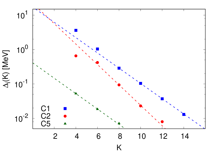
(a) SRG1.2

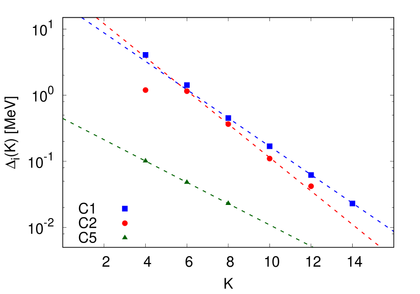
(b) SRG1.5

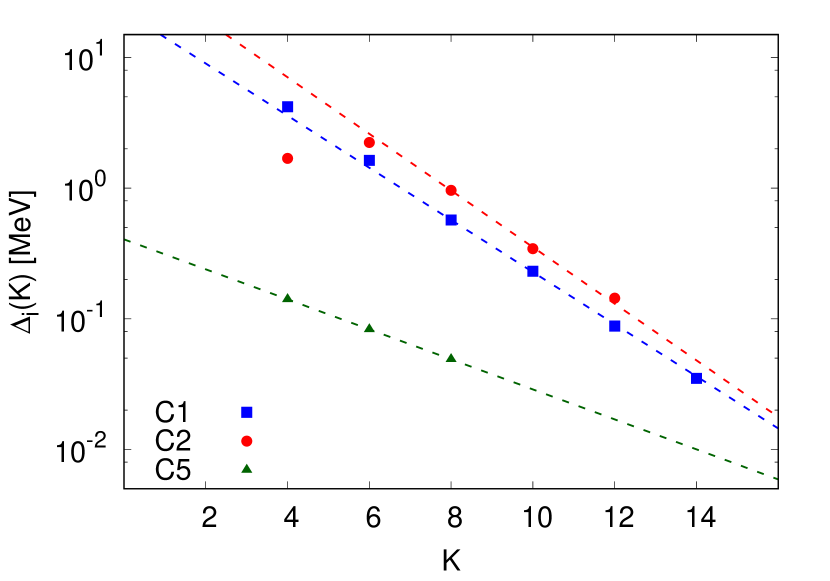
(c) SRG1.8

Figure 1: Values of $\Delta_{i}$ [see Eqs. (37)–(42)] for the classes C1 (squares), C2 (circles), and C5 (triangles) as function of the grandangular value K for the three SRG evolved potentials $\Lambda=1.2$ fm^-1 (a), $\Lambda=1.5$ fm^-1 (b), and $\Lambda=1.8$ fm^-1 (c). The dashed lines are the fits obtained using Eq. (44).

These effects can be seen also by comparing the values of $b_{i}$ obtained by the fits and reported in Table 5. For the classes C3, C4 and C6, the calculated values of $\Delta_{i}(K)$ are not enough to perform a fit and so we extract the parameter $b_{i}$ by using only the last two values of $\Delta_{i}$, namely

$$\frac{\Delta_{i}(K_{iM}-2)}{\Delta_{i}(K_{iM})}={\rm e}^{2b_{i}}\,.$$ (45)

This formula gives only a rough estimate of the convergence rate. The obtained values of $b_{i}$ are reported in Table 5 as well. For all the classes the values of $b_{i}$ decrease when $\Lambda$ grows which indicates a more and more repulsive core of the potential when $\Lambda$ increases.

Before discussing the calculation of the “missing” binding energy, we want to underline that Eq. (44) represents the asymptotic behavior of the convergence pattern when $K$ is large, while we are using value of $\Delta_{i}$ computed for not so large values of $K$. For this reason, for the final fit of class C1 and C2 we used only $\Delta_{i}(K)$ with $K\geq 8$. Indeed, in Figure 1 it is possible to observe that, for $K\leq 6$, $\Delta_{i}$ deviates from the fit. This is usual for the convergence of HH states, as already observed in the case of the $\alpha$ particle in Ref. Viviani et al. (2005), and is due to the fact that for small values of $K$ the number of states are not enough to give a good description of the wave function.

The “missing” binding energy due to the truncation of the expansion for each class to finite values of $K=K_{iM}$ can be defined as in Ref. Viviani et al. (2005)

$$\left(\Delta B\right)_{i}=\sum_{K=K_{iM}+2,K_{iM}+4,\dots}\Delta_{i}(K)\,,$$ (46)

and, by using Eq. (44), we obtain

$$\left(\Delta B\right)_{i}=\Delta_{i}(K_{iM})\frac{1}{{\rm e}^{2b_{i}}-1}\,.$$ (47)

The “total missing” binding energy is then computed as

$$\left(\Delta B\right)_{T}=\sum_{i=1,6}\Delta_{i}(K_{iM})\frac{1}{{\rm e}^{2b_{i}}-1}\,.$$ (48)

In Table 5 we summarize the “missing” binding energy of each class and the “total missing” binding energy. By inspecting the table we observe that the “total missing” binding energy is less than $1\%$ of the total binding energy for all the SRG evolved potentials. This confirms the high accuracy of the computed binding energies. As regarding the errors on the “missing” binding energy ($\delta(\Delta B)_{i}$), in the case of the class C1, C2 and C5 we propagate the errors on $b_{i}$ evaluated in the fits. The estimate of the “missing” binding energy suffers of the fact that the extrapolation is not really done for large $K$, in particular for the class C3, C4 and C6. Therefore, for these classes we consider a conservative error of $\delta(\Delta B)_{i}/(\Delta B)_{i}=0.5$. The error on the “total missing” binding energy is then computed as

$$\delta(\Delta B)_{T}=\sqrt{\sum_{i=1,6}\left(\delta(\Delta B)_{i}\right)^{2}}$$ (49)

For all the potentials considered, the relative error $\delta(\Delta B)_{T}/(\Delta B)_{T}$ is of the order of $\sim 20\%$.

		SRG1.2			SRG1.5			SRG1.8
$i$	$K_{iM}$	$\Delta_{i}(K_{iM})$	$b_{i}$	$(\Delta B)_{i}$	$\Delta_{i}(K_{iM})$	$b_{i}$	$(\Delta B)_{i}$	$\Delta_{i}(K_{iM})$	$b_{i}$	$(\Delta B)_{i}$
1	14	0.013	0.51	0.007(0)	0.023	0.49	0.014(0)	0.035	0.46	0.023(0)
2	12	0.008	0.68	0.003(1)	0.042	0.58	0.019(0)	0.144	0.50	0.084(11)
3	10	0.015	0.37	0.014(7)	0.022	0.32	0.024(12)	0.024	0.30	0.029(15)
4	10	0.008	0.60	0.004(2)	0.022	0.49	0.013(6)	0.045	0.38	0.039(20)
5	8	0.007	0.52	0.004(0)	0.023	0.37	0.021(0)	0.049	0.26	0.070(1)
6	8	0.004	0.44	0.003(1)	0.018	0.26	0.026(13)	0.048	0.11	0.19(9)
$(\Delta B)_{T}$				0.034(7)			0.117(19)			0.43(9)

Table 5: Increments of the ${}^{6}{\rm Li}$ binding energy $\Delta_{i}(K_{iM})$, computed using Eqs. (37)–(42) for the various classes $i=1,\dots,6$ and the SRG evolved potentials. The coefficients $b_{i}$ are fitted on the $\Delta_{i}(K)$ for the classes $i=1,2,5$ and computed as in Eq. (45) for the classes $i=3,4$ and $6$. $(\Delta B)_{i}$ is computed as in Eq. (46) and it represents the “missing” binding energy of each class, due to the truncation of the expansion up to a given $K_{iM}$. Finally, the “total missing” binding energy $(\Delta B)_{T}$ is computed from Eq. (48). Between the parenthesis we report the errors. With $(0)$ we indicate that the errors are smaller than the precision of the digits reported in the table.

In Table 6 we compare our results with those of Ref. Jurgenson et al. (2011), obtained using the NCSM. As it can be observed by inspecting column one and two, the results obtained with the same N3LO500-SRG$\Lambda$ potentials in Ref. Jurgenson et al. (2011), seem to be systematically larger. A possible explanation can be found in the fact that in Ref. Jurgenson et al. (2011), the Coulomb potential is included in the SRG evolution. By performing the calculations with the Coulomb interactions included in the SRG evolutions (indicated with IC in Table 6) we gain $\sim 30-40$ keV, solving partially the discrepancy. However our results remain still systematically smaller than the ones of Ref. Jurgenson et al. (2011), even if for $\Lambda=1.2$ fm^-1 and $\Lambda=1.8$ fm^-1 they are compatible within the error bars. A possible explanation of the remaining differences could be that we are using a slightly different SRG evolved potential.

	NIC (HH)		IC (HH)		Ref. Jurgenson et al. (2011) (NCSM)
	$B$	$B_{ex.}$	$B$	$B_{ex.}$	$B_{ex.}$
SRG1.2	31.75	31.78(1)	31.78	31.81(1)	31.85(5)
SRG1.5	32.75	32.87(2)	32.79	32.91(2)	33.00(5)
SRG1.8	32.21	32.64(9)	32.25	32.68(9)	32.8(1)

Table 6: Values of the computed ($B$) and extrapolated ($B_{ex.}$) ${}^{6}{\rm Li}$ binding energy, calculated with the HH basis including (IC) and not including (NIC) the Coulomb interaction in the SRG evolution. Here we report for comparison the extrapolated values of Ref. Jurgenson et al. (2011), obtained with the NCSM basis up to $N_{max}=10$. All the results are expressed in MeV.

IV.3 Electromagnetic static properties

In order to fully characterize the ${}^{6}{\rm Li}$ ground state we compute the value of charge radius, magnetic dipole moment and electric quadrupole moment. Since the wave function we use is not the “bare” wave function, we should take care of the SRG transformation of the operators in order to be fully consistent. However, it has been argued that long-range operators would not be affected by it Stetcu et al. (2005). Therefore, in this section we assume that

$$\hat{O}\approx\hat{O}(\Lambda)\,,$$ (50)

where $\hat{O}$ is the “bare” operator and $\hat{O}(\Lambda)$ the SRG evolved one. In any case we will verify this approximation by computing the operators for different values of $\Lambda$. Moreover, we discuss the convergence of these observables as function of $K$. From now on, with $K$ we indicate the fact that for each class we include all the HH states with $K_{i}\leq K$. In the case $K>K_{iM}$ for a given class C$i$, we include HH states of this class up to $K_{iM}$.

IV.3.1 Charge radius

The mean square (ms) charge radius of a nucleus is given by Friar et al. (1997)

$$\langle r_{c}^{2}\rangle=\langle r_{p}^{2}\rangle+\langle R_{p}^{2}\rangle+\frac{N}{Z}\langle R_{n}^{2}\rangle+\frac{3\hbar^{2}}{2m_{p}^{2}c^{2}}\,,$$ (51)

where $\langle R_{p}^{2}\rangle$ and $\langle R_{n}^{2}\rangle$ are the ms charge radii of proton and neutron respectively, and the last term is the Darwin-Foldy relativistic correction Foldy and Wouthuysen (1950). The values used for these three contributions are obtained from Ref. Tanabashi and et al. (2018). Moreover, $\langle r_{p}^{2}\rangle$ is the ms value of the proton point radius operator which for the ${}^{6}{\rm Li}$ is defined as

$${\hat{r}}_{p}^{2}=\frac{1}{3}\sum_{i=1}^{6}(\boldsymbol{r}_{i}-\boldsymbol{R}_{\text{c.m.}})^{2}\left(\frac{1+\tau_{z}(i)}{2}\right)\,,$$ (52)

where $\boldsymbol{R}_{\text{c.m.}}$ is the c.m. position, $\boldsymbol{r}_{i}$ the position of the particle $i$, and 3 the number of protons.

In Figure 2 we plot the values of the root mean square charge radius $r_{c}=\sqrt{\langle r_{c}^{2}\rangle}$ as function of $K$. From the figure we can observe an exponential behavior as $K$ increases. In order to extrapolate the full converged value, we fit our results with

$$r_{c}(K)=r_{c}(\infty)+a{\rm e}^{-bK}\,,$$ (53)

where $r_{c}(\infty)$ is the extrapolated value for $K\rightarrow\infty$. The final results are reported in Table 7.

	$r_{c}(\infty)$ [fm]
SRG1.2	2.47(1)
SRG1.5	2.42(2)
SRG1.8	2.52(10)
Exp.	2.540(28)

Table 7: Extrapolated values for the ${}^{6}{\rm Li}$ charge radii obtained using SRG evolved potentials with $\Lambda=1.2$, $1.5$ and $1.8$ fm^-1. In the last row we report for comparison the experimental value Puchalski and Pachucki (2013).

From the fit we have excluded the values of $r_{c}$ obtained for $K=2$ and $K=14$, since they do not follow the exponential behavior, as it can be seen in Figure 2. This is due to the fact that for $K=2$ there are not enough states to well define the structure of ${}^{6}{\rm Li}$, and among the states with $K=14$ we are not considering channels with $D$ states which are fundamental for describing properly the ${}^{6}{\rm Li}$ radius.

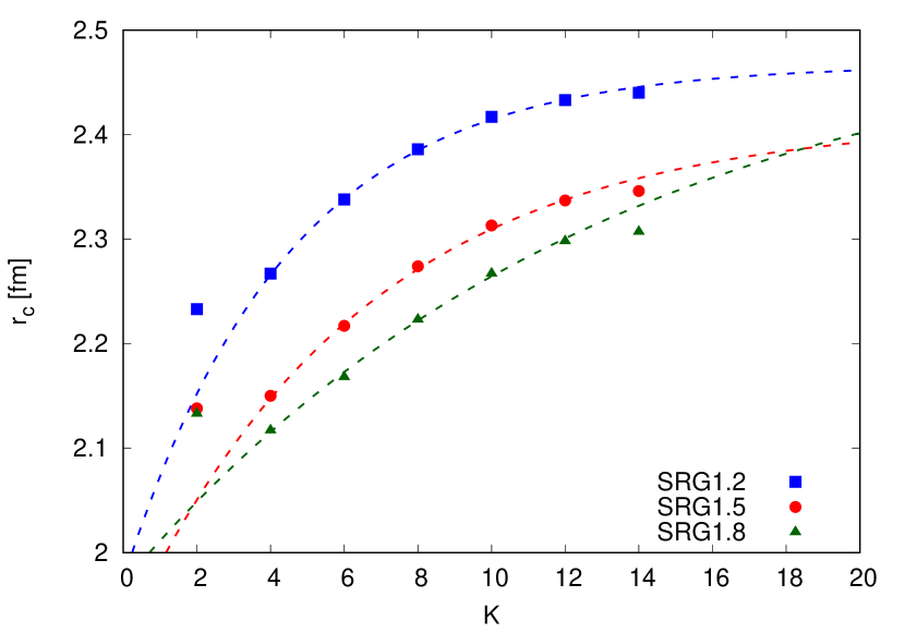
Figure 2: ${}^{6}{\rm Li}$ charge radius in fm as function of $K$ for the potential models SRG1.2 (blue), SRG1.5 (red), SRG1.8 (green). The exponential fit performed using Eq. (53) is also shown (dashed lines).

As it can be seen from Figure 2, the convergence is quite slow. Indeed, the HH basis is a “compact” basis and it is not able to describe perfectly the tail of the wave function which has a $\alpha+d$ dominant structure. We will treat this point with more details in Section IV.4. By comparing the results for the various SRG parameters, it is clear that the convergence rate is faster for the smallest values of the parameter $\Lambda$, since in these cases the correlations between the nucleons are reduced, favoring the convergence. The approximation of Eq. (50) for this observable is quite reliable since the difference on the extrapolations for the various $\Lambda$ is less than $\sim 4\%$.

IV.3.2 Magnetic dipole moment

The magnetic dipole moment operator for the $A=6$ case can be written as

$${\hat{\mu}_{z}}=\mu_{p}{\hat{\sigma}_{z}^{p}}+\mu_{n}{\hat{\sigma}_{z}^{n}}+{\hat{L}_{z}}\,.$$ (54)

where $\mu_{p}$ and $\mu_{n}$ are the proton and neutron intrinsic magnetic moment taken from Ref. Tanabashi and et al. (2018),

$${\hat{\sigma}_{z}^{p/n}}=\sum_{i=1}^{6}\sigma_{z}(i)\frac{1\pm\tau_{z}(i)}{2}\,$$ (55)

is the total spin of protons and neutrons and

$${\hat{L}_{z}^{p}} =\sum_{i=1}^{6}\ell_{z}(i)\frac{1+\tau_{z}(i)}{2}\,$$ (56)

is the angular momentum of the protons. The convergence of this operator as function of $K$ does not show an exponential behavior as in charge radius case but is quite fast since, it depends only on the percentage of the various partial waves, which are very stable being integral quantities. In Table 8 we report the mean values of the magnetic dipole moment obtained in the full configuration at $K=14$. Since we cannot give a reliable extrapolation to $K\rightarrow\infty$, as we have done for the charge radius, we consider a conservative theoretical error defined as

$$\Delta\mu_{z}=\max_{K=8,10,12}\left\{|\mu_{z}(K)-\mu_{z}(14)|\right\}\,,$$ (57)

where $\mu_{z}(K)$ is the value of the dipole magnetic moment of the ${}^{6}{\rm Li}$ wave function computed using $K$ as maximum value for the grandangular momentum.

	$\mu_{z}({}^{6}{\rm Li})[\mu_{N}]$	$\mu_{z}(d)[\mu_{N}]$
SRG1.2	0.865(1)	0.872
SRG1.5	0.858(2)	0.868
SRG1.8	0.852(2)	0.865
Exp.	0.822	0.857

Table 8: Values of the magnetic dipole moment $\mu_{z}$ for ${}^{6}{\rm Li}$ evaluated using SRG evolved potential models with $\Lambda=1.2$, $1.5$ and $1.8$ fm^-1. We reported also the value of the magnetic dipole moment of deuteron $\mu_{z}(d)$ computed with the same potentials. In the last row the experimental values are listed Stone (2014).

As it can be seen by inspecting the table, the value of the magnetic dipole moment slightly decreases by increasing the value of $\Lambda$. Indeed, when $\Lambda$ increases the correlations induced by the nuclear potential are stronger, generating a larger amount of $D$ component in the wave function, which reduces the value of $\mu_{z}$. However, the differences between the various $\Lambda$ is $\sim 1\%$ confirming that Eq. (50) is a quite good approximation for this observable.

If we consider ${}^{6}{\rm Li}$ to be formed as a $\alpha+d$ cluster, we can expect that

$$\mu_{z}({{}^{6}{\rm Li}})\approx\mu_{z}(d)\,,$$ (58)

because the $\alpha$-particle has no magnetic dipole moment. However, the internal structure of ${}^{6}{\rm Li}$ plays a fundamental role decreasing the value of the magnetic dipole moment compared to the deuteron one, as it can be observed comparing the experimental values (last row of Table 8). In Table 8 we compare the results of the magnetic dipole moment of ${}^{6}{\rm Li}$ and $d$ computed with the same SRG potentials. In all the cases, the ${}^{6}{\rm Li}$ magnetic dipole moment is reduced compared to the $d$ ones, showing that the potential models are going in the right direction, even if they are not able to reproduce the experimental value. Obviously this is partially due to the fact we are not considering the evolved operator and also that we are not including three-body forces. Moreover, as it was shown in Refs. Carlson and Schiavilla (1998); Schiavilla et al. (2019) for ${}^{3}{\rm H}$ and ${}^{3}{\rm He}$, the magnetic dipole moment receives important contributions from two-body electromagnetic currents. Therefore, we can expect that similar corrections are necessary in this case to reproduce the experimental value of $\mu_{z}({}^{6}{\rm Li})$.

IV.3.3 Electric quadrupole moment

The electric quadrupole moment operator for $A=6$ is defined as

$${\hat{Q}}=\sum_{i=1}^{6}(3z_{i}^{2}-r_{i}^{2})\left(\frac{1+\tau_{z}(i)}{2}\right)\,.$$ (59)

The study of this observable is crucial for understanding the goodness of the ${}^{6}{\rm Li}$ wave function we computed. Indeed, from the experiment, we know that the electric quadrupole moment of ${}^{6}{\rm Li}$ is very small and negative. For this reason, it is challenging for all the potential models to reproduce this value.

The convergence of this operator as function of $K$ shows an irregular trend due to large cancellations among the contributions coming from different sets of HH states. Therefore, as for the magnetic dipole moment, we report in Table 9 the value of this operator obtained for $K=14$ and the errors computed as given in Eq. (57) substituting the dipole magnetic moment with the electric quadrupole moment.

	$Q$ [$e$ fm2]
SRG1.2	-0.191(7)
SRG1.5	-0.101(7)
SRG1.8	-0.055(3)
Exp.	-0.0806(6)

Table 9: Values of the ${}^{6}{\rm Li}$ electric quadrupole moment obtained for SRG evolved potential models with $\Lambda=1.2$, $1.5$ and $1.8$ fm^-1. In the last row we report for comparison the experimental value Stone (2014).

The values obtained for the SRG potentials are quite dependent on the value of the parameter $\Lambda$. Therefore, for the electric quadrupole moment the approximation of Eq. (50) seems not to be valid. However, all the considered SRG evolved potentials are able to reproduce a small and negative value for the electric quadrupole moment. In particular, for $\Lambda=1.5$ and 1.8 fm^-1, we obtain values quite close to the experimental value of $-0.0806(6)\,e$ fm.

In order to understand why we have these differences between the various SRG evolved potentials, we report in Table 10 the partial wave contributions to this observable. As it can be seen, we have large differences only in the contribution coming from matrix element between $S$- and $D$-waves. In particular the value of this matrix element increases when $\Lambda$ increases. Therefore, the value of the electric quadrupole moment seems directly connected to the strength of the tensor term in the nuclear potential. Indeed, we can expect that if the correlations between $S$- and $D$-waves grow (as in the case of “bare” chiral potentials), the value of the electric quadrupole moment could come positive. Therefore, also in this case, the two-body current corrections to this observable could be necessary to explain the observed value of ${}^{6}{\rm Li}$ electric quadrupole moment.

	$S-D$	$D-D$	$P-P$	$P-D$	remaining
SRG1.2	$-0.187$	$-0.023$	$0.009$	$0.009$	$<0.001$
SRG1.5	$-0.102$	$-0.023$	$0.014$	$0.010$	$<0.001$
SRG1.8	$-0.058$	$-0.024$	$0.016$	$0.010$	$\phantom{<}0.001$

Table 10: Partial wave contributions to the ${}^{6}{\rm Li}$ electric quadrupole moment obtained using SRG evolved potentials with $\Lambda=1.2$, $1.5$ and $1.8$ fm^-1. All the values are given in unit of $e$ fm².

IV.4 Asymptotic Normalization Coefficients

The asymptotic normalization coefficients (ANCs) are properties of the bound state wave functions that can be related to experimental observables. In particular, in the case of the $\alpha+d$ radiative capture, it plays a fundamental role in the determination of the cross section. Moreover, the ANCs provide a test of quality of the variational wave function in the asymptotic region where the 4+2 clusterization is dominant.

In the asymptotic region, where the ${}^{6}{\rm Li}$ is clustered, the ${}^{6}{\rm Li}$ wave function results as

$${\Psi}_{{}^{6}{\rm Li}}\rightarrow C_{0}\frac{W_{-\eta,1/2}(2kr)}{r}\Psi_{\alpha+d}^{(0)}+C_{2}\frac{W_{-\eta,5/2}(2kr)}{r}\Psi_{\alpha+d}^{(2)}\,.$$ (60)

The function $\Psi^{(L)}_{\alpha+d}$ is the $\alpha+d$ cluster wave function which is defined as

$$\Psi^{(L)}_{\alpha+d}=\frac{1}{\sqrt{15}}{\cal A}\left[\left(\Psi_{\alpha}\times\Psi_{d}\right)_{1}Y_{L}(\hat{r})\right]_{1}\,,$$ (61)

where the symbol ${\cal A}$ is the antisymmetrization operator, $\Psi_{\alpha}$ and $\Psi_{d}$ are the wave functions of the $\alpha$-particle and the deuteron calculated in the HH variational approach, and $\boldsymbol{r}$ is the distance between the c.m. of the $\alpha$-particle and the deuteron. In the previous equation, the spin 0 of the $\alpha$-particle is combined with spin 1 of the deuteron giving a “channel” spin $S=1$. The channel spin is then coupled with the angular momentum $L$ to give a total angular momentum $J=1$. Because of the even parity of ${}^{6}{\rm Li}$, $\alpha$ and $d$, the $\alpha+d$ cluster can be only in states $L=0,2$. In Eq. (60), $W_{-\eta,L+1/2}(2kr)$ is the Whittaker function with $k$ and $\eta$ determined as

$$k=\sqrt{\frac{8}{3}\frac{m}{\hbar^{2}}B_{c}}\,,\quad\eta=\frac{3}{4}\frac{m}{\hbar^{2}}\frac{e^{2}}{k}\,.$$ (62)

Here we have used $e^{2}=1.44$ MeV fm, $\hbar^{2}/m=41.47$ MeV fm², and $B_{c}=B_{{}^{6}{\rm Li}}-B_{\alpha}-B_{d}$ with $B_{{}^{6}{\rm Li}}$, $B_{\alpha}$ and $B_{d}$ the ${}^{6}{\rm Li}$, $\alpha$ and $d$ binding energy, respectively. Finally, $C_{0/2}$ of Eq. (60) are the $L=0$ and $L=2$ ANCs, respectively.

In order to compute $C_{L}$, we have defined the $\alpha+d$ overlap as

$$f_{L}(r)=r\frac{\langle\Psi_{{}^{6}{\rm Li}}|\Psi^{(L)}_{\alpha+d}\rangle_{r}}{\left[\langle\Psi_{d}|\Psi_{d}\rangle\langle\Psi_{\alpha}|\Psi_{\alpha}\rangle\langle\Psi_{{}^{6}{\rm Li}}|\Psi_{{}^{6}{\rm Li}}\rangle\right]^{1/2}}\,,$$ (63)

where we have defined the proper norms of a generic wave function of $A$ bodies as

$$\langle\Psi_{A}|\Psi_{A}\rangle =\int\prod_{i=1}^{A}d\boldsymbol{r}_{i}\,\delta\left(\boldsymbol{R}^{A}_{\text{c.m.}}-\frac{1}{A}\sum_{j=1}^{A}\boldsymbol{r}_{j}\right)|\Psi_{A}|^{2}=1\,,$$ (64)

and $\boldsymbol{R}_{\text{c.m.}}^{A}$ is the generic position of the c.m. of the $A$ particles. Moreover, in Eq. (63) we indicate with $\langle\rangle_{r}$ the fact that we are performing the spin-isospin traces and the integration over all the position of the particles except the intercluster distance $r$ and the center of mass. With such definition the overlap is completely independent on the choice of the internal variables. To perform the calculation it is convenient to introduce the proper set of Jacobi coordinates (set “B”) to describe the $\alpha+d$ clusterization, defined as

$$\boldsymbol{\xi}_{1Bp} =\boldsymbol{r}_{n}-\boldsymbol{r}_{m}$$ (65)

$$\boldsymbol{\xi}_{2Bp} =\sqrt{\frac{8}{3}}\left(\frac{\boldsymbol{r}_{n}+\boldsymbol{r}_{m}}{2}-\frac{\boldsymbol{r}_{l}+\boldsymbol{r}_{k}+\boldsymbol{r}_{j}+\boldsymbol{r}_{i}}{4}\right)$$

$$\boldsymbol{\xi}_{3Bp} =\sqrt{\frac{3}{2}}\left(\boldsymbol{r}_{l}-\frac{\boldsymbol{r}_{k}+\boldsymbol{r}_{j}+\boldsymbol{r}_{i}}{3}\right)$$

$$\boldsymbol{\xi}_{4Bp} =\sqrt{\frac{4}{3}}\left(\boldsymbol{r}_{k}-\frac{\boldsymbol{r}_{j}+\boldsymbol{r}_{i}}{2}\right)$$

$$\boldsymbol{\xi}_{5Bp} =\boldsymbol{r}_{j}-\boldsymbol{r}_{i}\,.$$

Then, the overlap function reduces to

$$f_{L}(r) =r\sqrt{15}\left(\frac{\sqrt{6}}{4}\right)^{\frac{3}{2}}\int\prod_{i=1}^{5}d\boldsymbol{\xi}_{iB}\,\delta\left(r-\sqrt{\frac{3}{8}}\xi_{2B}\right)$$ (66)

$$\times\Psi_{{}^{6}{\rm Li}}(\boldsymbol{\xi}_{1B},\boldsymbol{\xi}_{2B},\boldsymbol{\xi}_{3B},\boldsymbol{\xi}_{4B},\boldsymbol{\xi}_{5B},\boldsymbol{\xi}_{6B})^{\dagger}$$

$$\times\left[\left(\Psi_{\alpha}(\boldsymbol{\xi}_{3B},\boldsymbol{\xi}_{4B},\boldsymbol{\xi}_{5B})\times\Psi_{d}(\boldsymbol{\xi}_{1B})\right)_{1}Y_{L}(\hat{r})\right]_{1}\,,$$

where we have used the antisymmetry of the ${}^{6}{\rm Li}$ wave function to eliminate the antisymmetrization operator $\cal{A}$, and we have multiplied for a factor 15 to take care of the fact that the initial function $\Psi_{\alpha+d}^{(L)}$ contains such a number of $4+2$ partitions of the six particles. Finally, $\left(\sqrt{6}/{4}\right)^{\frac{3}{2}}$ is a factor that comes from the normalizations of the wave functions. In Eq. (66) we indicate with $\Psi_{\alpha}(\boldsymbol{\xi}_{3B},\boldsymbol{\xi}_{4B},\boldsymbol{\xi}_{5B})$ the wave function of the $\alpha$-particle constructed as the sum over the 12 even permutations of the particles $(1,2,3,4)$ and with $\Psi_{d}(\boldsymbol{\xi}_{1B})$ the wave function of the deuteron constructed with the particles $(5,6)$. The ${}^{6}{\rm Li}$ wave function is the one of Eq. (24) rewritten in terms of the set “B” of Jacobi coordinates, by redefining properly the TCs. The ANCs is then obtained by

$$C_{L}=\lim_{r\rightarrow\infty}C_{L}(r)\,,$$ (67)

where

$$C_{L}(r)=\frac{f_{L}(r)}{W_{-\eta,L+1/2}(2kr)}\,.$$ (68)

The dependence of the overlap to the truncation level of the HH expansion of ${}^{6}{\rm Li}$ is studied by varying the maximum value of $K$. In Figure 3 we plot the $L=0$ component of the overlap function obtained with the SRG1.5 potential. From the figure it is clear that the tail of the overlap has not the correct behavior of the Whittaker function (full red line). This is due to the limited number of HH states used in the expansion of the ${}^{6}{\rm Li}$ wave function, which are not enough to reproduce the correct asymptotic behavior. However, it is also clear that the HH states are slowly constructing the correct asymptotic slope when $K$ increases. In reverse, for the short-range part ($r<3$ fm) the convergence is fast and completely reached. Similar comments apply also for all the other potentials and the $L=2$ component.

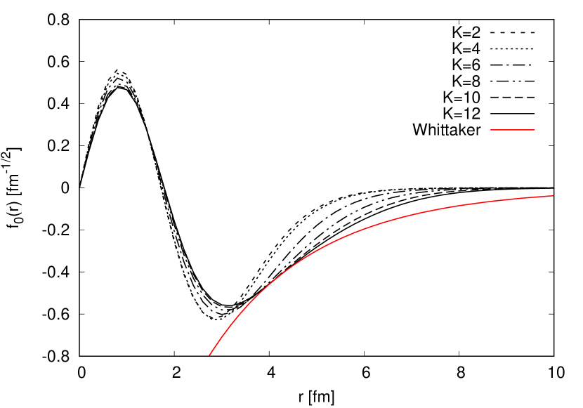
Figure 3: $S$-wave component of the overlap function $f_{L}(r)$ defined in Eq. (66) for different values of $K$ used in the expansion of the ${}^{6}{\rm Li}$ wave function. The full red line represents the correct asymptotic behavior given by the Whittaker function. These results are obtained with the SRG1.5 potential.

The results obtained for the $L=0$ and $L=2$ overlaps are qualitative consistent with the ones reported in Refs. Forest et al. (1996); Nollett et al. (2001); Navrátil (2004); Navrátil and Quaglioni (2011).

By using Eq. (68), we can then calculate the ANCs. In Figure 4 and 5 we illustrate with the dashed lines the ratio $C_{0}(r)$ and $C_{2}(r)$ computed in the SRG1.5 case, for $K=10$ (blue) and $K=12$ (red). Both the functions $C_{0}(r)$ and $C_{2}(r)$ shows a sort of “plateau” around the minimum (maximum in the case $L=2$), from which we can have a crude estimate of the ANC. We observe the same behavior for all the other potentials considered in this paper. In Table 11 with Method I we indicate the estimate of the ANCs for both $L=0$ and $L=2$ components and the various SRG evolved potentials obtained with this approach. The numerical differences among the ANCs obtained from the three potentials are mostly due to the different values of $k$, present in $\eta$ [see Eq. (62)], entering in the Whittaker function. The values of $B_{c}$, from which the value of $k$ depends, are reported as well in Table 11.

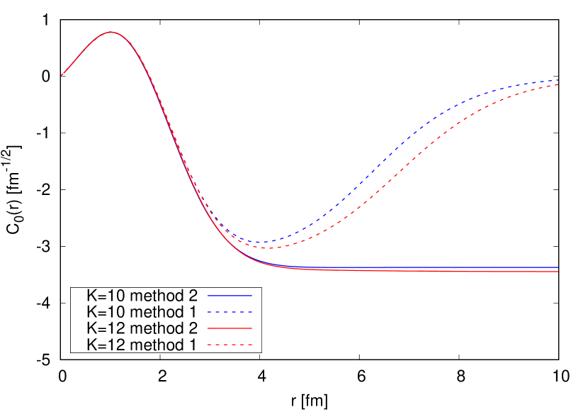
Figure 4: Function $C_{0}(r)$ computed with the overlap method (dashed lines) and the equation method (continuous lines) for the SRG1.5 potential. The calculations are performed with the ${}^{6}{\rm Li}$ wave function computed with $K=10$ (blue lines) and $K=12$ (red lines). Results of the equation method are obtained using ${\overline{K}}=8$.

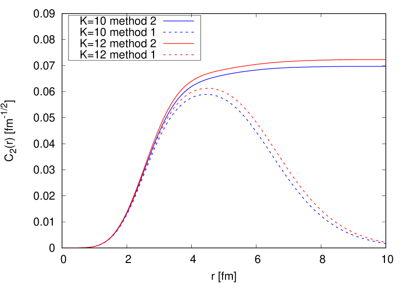
Figure 5: The same as Figure 4, but for the function $C_{2}(r)$.

	Model	$B_{c}$ [MeV]	$C_{0}$ [fm-1/2]	$C_{2}$ [fm-1/2]	$C_{2}/C_{0}$
	SRG1.2	3.00(1)	$-3.9$	$0.10$	$-0.03$
Method 1	SRG1.5	2.46(2)	$-3.0$	$0.06$	$-0.02$
	SRG1.8	2.01(9)	$-2.3$	$0.03$	$-0.01$
	SRG1.2	3.00(1)	$-4.19(12)$	0.116(18)	$-0.028(5)$
Method 2	SRG1.5	2.46(2)	$-3.44(7)$	0.072(15)	$-0.021(5)$
	SRG1.8	2.01(9)	$-3.01(7)$	0.047(10)	$-0.016(4)$
Ref. Nollett et al. (2001)	AV18/UIX	1.47	$-2.26(5)$	–	$-0.027(1)$
Ref. Hupin et al. (2015)	SRG1.5(3b)	1.49	$-2.695$	0.074	$-0.027$
Ref. George and Knutson (1999)	Exp.	1.4743	$-2.91(9)$	0.077(18)	$-0.025(11)$

Table 11: Values of the ANC $C_{0}$ and $C_{2}$ in fm^-1/2 for the various SRG evolved potentials with $\Lambda=1.2$, $1.5$ and $1.8$ fm^-1 and the two methods used for their calculation. We report also the binding energy $B_{c}$ (MeV) used in the calculation of the ANC and the ratio $C_{2}/C_{0}$. For completeness, we shows also the results of the ab-initio calculation of Ref. Nollett et al. (2001) obtained with AV18/UIX potential, and of Ref. Hupin et al. (2015) obtained with the SRG1.5 including three-body forces (3b). Also the experimental values of Ref. George and Knutson (1999) are listed.

From the overlap it is also possible to compute the spectroscopic factor ${\cal S}_{L}$ defined as

$${\cal S}_{L}=\int_{0}^{\infty}dr\,f_{L}(r)^{2}\,,$$ (69)

which can be interpreted as the percentage of $\alpha+d$ clusterization in the ${}^{6}{\rm Li}$ wave function. In Table 12 we report the values of the spectroscopic factors obtained for the various potentials. Independently on the $\Lambda$ parameter used, it results that ${}^{6}{\rm Li}$ is clustered in an $\alpha+d$ system for more than $80\%$. The differences between the values obtained with the SRG evolved potentials can be due to the fact that the induced and proper three-body forces are not included. Moreover, in the table we compare our results with the calculation of Refs. Forest et al. (1996); Nollett et al. (2001); Navrátil (2004). The values are similar, even if obtained with different potential models, and compatible with the experimental estimate of Ref. Robertson et al. (1981).

Method	Potential	${\cal S}_{0}$	${\cal S}_{2}$	${\cal S}_{0}+{\cal S}_{2}$
HH (This work)	SRG1.2	0.909	0.008	0.917
	SRG1.5	0.868	0.007	0.875
	SRG1.8	0.840	0.006	0.846
GFMC (Ref. Forest et al. (1996))	AV18/UIX	$0.82$	$0.021$	0.84
GFMC (Ref. Nollett et al. (2001))	AV18/UIX	$-$	$-$	0.87(5)
NCSM (Ref. Navrátil (2004))	CD-B2k	0.822	0.006	0.828
Exp. (Ref. Robertson et al. (1981))		$-$	$-$	0.85(4)

Table 12: Values of the spectroscopic factors for the various SRG-evolved potentials with $\Lambda=1.2$, 1.5, and 1.8 fm^-1. In the last rows we compare our results with the results obtained within the GFMC using the AV18/UIX interaction, the result obtained within the NCSM using a unitary transformed version of the CD-Bonn2000 (CD-B2k) potential Machleidt (2001), and the experimental one.

Since the procedure adopted so far for extrapolating the ANCs results to be somewhat unsatisfactory, due to the difficult identification of the “plateau”, we use another procedure, based on Ref. Timofeyuk (1998) and already applied in Ref. Viviani et al. (2005). With this approach, we can extrapolate the ANCs with greater accuracy. Assuming that $\Psi_{\alpha}$ and $\Psi_{d}$ are “exact”, it is not difficult to show that the overlap function $f_{L}(r)$ should satisfy the equation

$$\left[-\frac{\hbar^{2}}{2\mu}\left(\frac{d^{2}}{dr^{2}}-\frac{L(L+1)}{r^{2}}\right)+\frac{2e^{2}}{r}+B_{c}\right]f_{L}(r)+g_{L}(r)=0\,,$$ (70)

where $\mu=4/3m$ is the reduced mass of the $\alpha+d$ system, and

$$g_{L}(r) =r\sqrt{15}\left(\frac{\sqrt{6}}{4}\right)^{\frac{3}{2}}\int\prod_{i=1}^{5}d\boldsymbol{\xi}_{iB}\,\delta\left(r-\sqrt{\frac{8}{3}}\xi_{2B}\right)$$ (71)

$$\times\Psi_{{}^{6}{\rm Li}}(\boldsymbol{\xi}_{1B},\dots,\boldsymbol{\xi}_{5B})^{\dagger}\left(\sum_{i\in\alpha}\sum_{j\in d}V_{ij}-\frac{2e^{2}}{r}\right)$$

$$\times\left[\left(\Psi_{\alpha}(\boldsymbol{\xi}_{3B},\boldsymbol{\xi}_{4B},\boldsymbol{\xi}_{5B})\times\Psi_{d}(\boldsymbol{\xi}_{1B})\right)_{1}Y_{L}(\hat{r})\right]_{1}\,,$$

is the so called source term with $V_{ij}$ the two-body potential. As $r\rightarrow\infty$, the function $g_{L}(r)\rightarrow 0$, and the solution of Eq. (70) coincides with the Whittaker function, allowing for the extraction of the ANC using Eq. (67).

Since the calculation of $g_{L}(r)$ in this form is quite involved, we want to rewrite it so that we can use the same HH properties we used to compute the potential matrix element of Eq. (26). In order to do that, we eliminate the $\delta$-function in Eq. (71) expanding $g_{L}(r)$ in terms of the Laguerre polynomials, i.e.

$$g_{L}(r)=\sum_{n=0}^{N_{\text{max}}}C_{n}^{L}\overline{f}_{n}(r)\,,$$ (72)

where

$$\overline{f}_{n}(r)=\gamma_{a}^{\frac{3}{2}}\sqrt{\frac{n!}{(n+2)!}}L_{n}^{(2)}(\gamma_{a}r)\mathrm{e}^{-\frac{\gamma_{a}r}{2}}\,.$$ (73)

The parameter $\gamma_{a}$ is chosen to optimize the expansion. Then, the coefficients $C_{n}^{L}$ are given by

$$C_{n}^{L}=\int dr\,r^{2}g_{L}(r)\overline{f}_{n}(r)\,,$$ (74)

and, substituting Eq. (71) in Eq. (74), we obtain

$$C_{n}^{L} =\sqrt{15}\left(\frac{\sqrt{6}}{4}\right)^{\frac{3}{2}}\int\prod_{i=1,5}d\boldsymbol{\xi}_{iB}\,\Psi_{{}^{6}{\rm Li}}(\boldsymbol{\xi}_{1B},\dots,\boldsymbol{\xi}_{5B})^{\dagger}$$ (75)

$$\times\left(\sum_{i\in\alpha}\sum_{j\in d}V_{ij}-\frac{2e^{2}}{r}\right)\big{[}(\Psi_{\alpha}(\boldsymbol{\xi}_{3B},\boldsymbol{\xi}_{4B},\boldsymbol{\xi}_{5B})$$

$$\times\Psi_{d}(\boldsymbol{\xi}_{1B}))_{1}Y_{L}(\hat{r})\big{]}_{1}\overline{f}_{n}(r)\Big{|}_{\boldsymbol{r}=\sqrt{\frac{3}{8}}{\boldsymbol{\xi}}_{2B}}\,.$$

If now we define the 4+2 cluster wave function as

$$\Psi_{L,n}=\left[\left(\Psi_{\alpha}(\boldsymbol{\xi}_{3B},\boldsymbol{\xi}_{4B},\boldsymbol{\xi}_{5B})\times\Psi_{d}(\boldsymbol{\xi}_{2B})\right)_{1}Y_{L}(\hat{r})\right]_{1}\overline{f}_{n}(r)\,.$$ (76)

it is possible to expand it in terms of the six-body HH states, namely

$$\Psi_{L,n}=\sum_{{\overline{l}}=0}^{{\overline{l}}_{max}}\sum_{{\overline{K}}=0}^{{\overline{K}}_{max}}\sum_{{\overline{L}}\,{\overline{S}}\,{\overline{T}},{\overline{\alpha}}}c^{{\overline{K}}\,{\overline{L}}\,{\overline{S}}\,{\overline{T}}}_{{\overline{l}},{\overline{\alpha}}}(L,n)\sum_{p_{\alpha}=1}^{12}\Phi^{{\overline{K}}\,{\overline{L}}\,{\overline{S}}\,{\overline{T}}}_{{\overline{l}},{\overline{\alpha}}}(p_{\alpha})\,,$$ (77)

where the function $\Phi^{{\overline{K}}\,{\overline{L}}\,{\overline{S}}\,{\overline{T}}}_{{\overline{l}},{\overline{\alpha}}}$ are the HH functions of Eq. (13) expressed in terms of the set “B” of Jacobi coordinates. Note that with $p_{\alpha}$ we indicate the even permutation of $(i,j,k,l)$ of the six particles $(i,j,k,l,5,6)$ which coincide with the 12 permutations of the four particles inside the $\alpha$ particle. In Eq. (77) the coefficients $c^{{\overline{K}}\,{\overline{L}}\,{\overline{S}}\,{\overline{T}}}_{{\overline{l}},{\overline{\alpha}}}(L,n)$ are obtained from

$$c^{{\overline{K}}\,{\overline{L}}\,{\overline{S}}\,{\overline{T}}}_{{\overline{l}},{\overline{\alpha}}}(L,n)=\langle\Phi^{{\overline{K}}\,{\overline{L}}\,{\overline{S}}\,{\overline{T}}}_{{\overline{l}},{\overline{\alpha}}}(p=1)|\Psi_{L,n}(p=1)\rangle_{\Omega_{B},\rho}\,,$$ (78)

where with $\langle\rangle_{\Omega_{B},\rho}$ we indicate the integration over all the internal variables and the spin-isospin traces. We want to underline that the calculation of these coefficients is very easy since it involves only the reference permutation ($p=1$). The equivalence in Eq. (77) holds exactly only when ${\overline{K}}_{max}\rightarrow\infty$ and ${\overline{l}}_{max}\rightarrow\infty$. Obviously this is not the case, but we can check the quality of our expansion by looking to the convergence of the observables when we increase ${\overline{K}}_{max}$ and ${\overline{l}}_{max}$. By replacing Eq. (77) in Eq. (75) the calculation of the source term reduces to compute a series of matrix elements of the potential between HH states, that can be easily done by following the procedure of Section II.

For the calculation of the source term we use $N_{\text{max}}=20$ for the expansion with the Laguerre polynomials of the source term [Eq. (72)] and ${\overline{l}}_{max}=40$ for the hyperradial part of the cluster function [Eq. (77)]. Both these values permit to reach full convergence in the respective expansions. More interesting is to study the convergence as function of ${\overline{K}}$. In Figure 6 we plot the source term $g_{L}(r)$ for the $L=0$ component in the case of the SRG1.5 potential for different values of ${\overline{K}}$. The calculation shown in this plot is performed by considering the ${}^{6}{\rm Li}$ wave function computed for $K=12$. From the figure it is immediately clear that we have a nice convergence in ${\overline{K}}$ for the short-range part ($r<3-4$ fm) but not for larger $r$. This effect is due to the fact that the Jacobi polynomials are not flexible enough in reproducing the exponential behavior of the cluster wave functions of Eq. (76). However, by inspecting the figure, it results clear that there are problems only in a region where $g_{0}(r)$ is a factor 100 smaller than the peak. A similar convergence behavior in ${\overline{K}}$ is found also for the other potentials studied and for $g_{2}(r)$.

Figure 6: The source term $g_{0}(r)$ for different values of ${\overline{K}}$ used in the projection of the $\alpha+d$ cluster wave functions. This figure is obtained by using SRG1.5 potential, and the ${}^{6}{\rm Li}$ wave function computed with $K=12$.

These considerations on $g_{L}(r)$ reflects directly on the calculated overlap via Eq. (70). Indeed, thanks to the fact that the term $g_{L}(r)$ vanishes for large $r$, we obtain the correct asymptotic behavior, namely the Whittaker function. In Figures 4 and 5 we compare the functions $C_{0}(r)$ and $C_{2}(r)$ obtained by solving the equation (full lines) with the ones obtained from the overlap (dashed lines). In the figures we report the results obtained for SRG1.5 where we used values of $K=10$ and $12$ for the calculation of the ${}^{6}{\rm Li}$ wave function and ${\overline{K}}=8$ for the expansion of the cluster wave function. From Figures 4 and 5 it is clear that in the short-range part ($r<2-3$ fm) the two approaches are essentially indistinguishable, proving the validity of our expansion of the cluster wave function in HH states. For larger $r$ the two approaches starts to diverge since the functions $C_{0}(r)$ and $C_{2}(r)$ computed with the direct overlap are not following the correct asymptotic behavior, as already discussed. Similar results are obtained also for the other two SRG evolved potentials. We observe that the “harder” is the potential, the smaller is the value of $r$ for which the disagreement between the two approaches starts to be important. This is an evidence of the fact that also the convergence in ${\overline{K}}$ depends on the potential.

From the equation method it is easy now to determine the ANCs with great accuracy as function of $K$ and ${\overline{K}}$ ($C_{L}(K,{\overline{K}})$). As function of ${\overline{K}}$ the ANCs have not a smooth convergence and this does not permits us to give a reliable extrapolation for ${\overline{K}}\rightarrow\infty$. Therefore, we consider as best values the ANCs obtained at ${\overline{K}}=8$ to which we add a conservative error of

$$\Delta C^{(0)}_{L}(K)=0.5\times|C_{L}(K,{\overline{K}}=6)-C_{L}(K,{\overline{K}}=8)|\,.$$ (79)

As regarding the expansion in $K$, the convergence is smooth and shows a clear exponential behavior. Therefore we fit the values $C_{L}(K,8)$ using

$$C_{L}(K,8)=C_{L}(\infty,8)+a{\rm e}^{-bK}\,.$$ (80)

Also for this expansion we consider a conservative error of

$$\Delta C_{L}^{(1)}=0.5\times|C_{L}(12,8)-C_{L}(\infty,8)|\,.$$ (81)

The total error on the final value $C_{L}(\infty,8)$ is

$$\Delta C_{L}=\sqrt{\left(\Delta C^{(0)}_{L}(12)\right)^{2}+\left(\Delta C^{(1)}_{L}\right)^{2}}\,.$$ (82)

In Table 11 with Method II we indicate our final results for $C_{L}(\infty,8)$. Also in this case the numerical differences among the ANCs for the three SRG-evolved potentials are due to the different binding energy $B_{c}$ used to compute the Whittaker functions. From the table it is also evident that the results obtained with the equation method are systematically larger than the one estimated by the overlap itself. Even if the results obtained with the equation are affected by significant errors due to the expansion in the HH states of the cluster wave functions, we consider these as more reliable. Indeed, those obtained from the overlap suffer from the difficulty of individuating unambiguously a well defined plateau and so of unknown systematical errors. For completeness in the table we report also the experimental values of Ref. George and Knutson (1999) and the calculation of Ref. Nollett et al. (2001) obtained with the Argonne $v_{18}$ (AV18) $NN$ interaction Wiringa et al. (1995) combined with the Urbana IX (UIX) $NNN$ potential Pudliner et al. (1997), and of Ref. Hupin et al. (2015) obtained with the SRG1.5 potential including three-body forces (3b). We cannot really perform a comparison, since our results do not contain the contribution of the three-body forces, and they are not computed at the physical energy $B_{c}$. However, from a qualitative point of view, the results are quite satisfactory, since for all the values of $\Lambda$, we are able to reproduce the correct magnitude of the experimental ANCs.

V The role of ${}^{6}{\rm Li}$ in the direct dark matter search

In recent years experiments devoted to the direct search of dark matter are planned to use light nuclei, and in particular lithium, as probes to search signal of light spin-dependent dark matter Abdelhameed et al. (2019). Usually, in the determination of the sensitivity limit, very old shell-model calculations for nuclei are considered. However, it is very well known that all shell-models fail to describe the ${}^{6}{\rm Li}$ structure. The aim of this section is to furnish reliable calculation of the necessary matrix elements.

The formula that is usually used to determine the rate of events for spin-dependent dark matter results to be proportional to $\langle S_{p/n}\rangle^{2}$ Lewin and Smith (1996), where $\langle S_{p/n}\rangle$ is the mean value of the proton (neutron) spin operator

$$\hat{S}_{p/n}=\frac{1}{2}\sum_{i=1}^{6}\sigma(i)\frac{1\pm\tau_{z}(i)}{2}\,,$$ (83)

on the nuclear wave function. In the case of ${}^{6}{\rm Li}$, if we consider it as a pure state of isospin $T=0$, by exploiting Wigner-Eckart theorem, it is easy to show that

$$\langle S_{p}\rangle_{{}^{6}{\rm Li}}=\langle S_{n}\rangle_{{}^{6}{\rm Li}}\,.$$ (84)

In order to give a very rough estimate of these matrix elements for ${}^{6}{\rm Li}$, we can consider it as a $\alpha+d$ cluster. If we suppose that $\alpha$ is a fully spin-0 particle, the only contribution to the spin of ${}^{6}{\rm Li}$ comes from the deuteron, namely

$$\langle S_{p}\rangle_{{}^{6}{\rm Li}}=\langle S_{n}\rangle_{{}^{6}{\rm Li}}\approx 0.5\,.$$ (85)

In our calculation we considered the full ${}^{6}{\rm Li}$ structure. In particular, by taking care of all the possible partial waves which compose the ${}^{6}{\rm Li}$ wave function (see Table 2), the spin operator results

$$\langle S_{p/n}\rangle_{{}^{6}{\rm Li}} =\frac{1}{2}P_{{}^{3}S_{1}}+\frac{1}{4}P_{{}^{1}P_{1}}+\frac{3}{4}P_{{}^{3}P_{1}}-\frac{1}{4}P_{{}^{3}D_{1}}+\frac{1}{4}P_{{}^{5}D_{1}}$$ (86)

$$+P_{{}^{7}D_{1}}-\frac{1}{2}P_{{}^{5}F_{1}}+\frac{1}{4}P_{{}^{7}F_{1}}-\frac{3}{4}P_{{}^{7}G_{1}}\,,$$

where $P_{i}$ is the percentage of the $i$-wave in the ${}^{6}{\rm Li}$ wave function. In Table 13 we present the results obtained for the proton (neutron) spin with the three different SRG evolved potentials used in this work. The errors are computed as in Eq. (57) by substituting the magnetic dipole moment with the spin operator.

	$\langle S_{p}\rangle(=\langle S_{n}\rangle)$
SRG1.2	0.479(1)
SRG1.5	0.472(2)
SRG1.8	0.464(3)

Table 13: Mean values of the proton (neutron) spin operator obtained using SRG evolved potentials with $\Lambda=1.2$, $1.5$ and $1.8$ fm^-1.

The differences among the three values and the result of Eq. (85) are directly related to the presence of $D$-wave components in ${}^{6}{\rm Li}$. Indeed, the larger are the $D$-wave components (and in particular the ${}^{3}D_{1}$), the smaller is the value of the spin operator. A similar dependence on the percentage of $D$-wave was already found in Ref. Körber et al. (2017) for the nuclear operators that are coupled to spinless dark matter.

VI Conclusions and perspectives

We have studied the solution of the Schrödinger equation for the six-nucleon ground state using the HH functions. The main problem in using the HH approach is the large degeneracy of the basis. Therefore, we performed a selection of the HH states that gives the most important contributions by following the same procedure used in Ref. Viviani et al. (2005) for the $\alpha$-particle ground state. The selection was performed by dividing the HH functions into classes depending on their total angular momentum and spin, as well as other quantum numbers. For each class we truncate the expansion so as to obtain the required accuracy.

Many modern $NN$ potentials contain a strong repulsive core which makes impossible to reach adequate accuracy with variational approaches in $A=6$ systems, because of the huge number of states needed in the wave function expansion. Therefore, in this work we limited our study to the N3LO500 chiral interaction of Ref. Entem and Machleidt (2003) evolved with the SRG unitary transformation. This permits to reach good accuracy with the HH available basis. In this first study we considered only two-body forces, even if the HH formalism is versatile enough to treat also three-body interactions without any additional problem. The inclusion of three-nucleon forces is currently in progress.

We have performed the calculation of the binding energy and of electromagnetic properties of ${}^{6}{\rm Li}$. Since we are not considering three-body forces, neither proper, nor induced by the SRG evolution, a meaningful comparison of our results with the experimental values is still premature. Regarding the electromagnetic properties of ${}^{6}{\rm Li}$, we have observed a strong dependence on the strength of the tensor forces. In future, we plan to include also the effect of two-body currents, necessary probably to explain the small and negative electric quadrupole moment of ${}^{6}{\rm Li}$. Finally, we have studied the $\alpha+d$ clusterization with the goal of determining the asymptotic normalization coefficients. In doing this, we performed a projection of the cluster wave function on the HH states. This approach can be used also in the study of scattering states, in order to simplify the calculation of the potential matrix elements. The calculation of the $\alpha+d$ scattering within this approach is also in progress.

This work was motivated in order to reach three goals. The first one is to show that the HH expansion applied to six-nucleon bound problem can reach the same level of precision of other approaches, as the NCSM, by using the same potentials. In this sense this work represents an important benchmark for both the HH and the NCSM techniques in the $A=6$ system. The second goal is the extension of this approach to work with “bare” chiral interactions also in the case of six-nucleon problem. All the results reported here were obtained by working on a single core with few tens of CPUs. Therefore, we expect possible to consider larger basis by using a more massive parallelization. We hope this will allow to reach a good accuracy also with a “bare” chiral interaction. Moreover, the selection of the classes can be improved reducing the number of states needed in the expansion. The third goal will be the possibility of use this algorithm for systems up to $A=8$. Also in this case a massive parallelization will be fundamental. However, also other approaches directly inspired by the NCSM method, as the inclusion of clustered component in the wave function, can be implemented in the HH formalism in order to improve the convergence.

Appendix A Technical details of the calculation

The biggest computational challenge for applying the HH formalism to the $A=6$ system is the calculation and the storage of the potential matrix elements, because of the high number of basis states needed to reach convergence. In this appendix we present the main feature of the algorithm that we implemented to compute the potential matrix elements exploiting the advantages of using the TC. The calculations have been performed in parallel machine using a single node with 48 Intel Xenon 8160 CPUs @2.10GHz.

Before starting to discuss the algorithm, let us give an idea of the dimension of the problem of computing the potential matrix elements in this formalism. We start from Eq. (30). The number of operations needed to compute the potential matrix elements of Eq. (30) for given sets $\gamma=\{K,L,S,T\}$ and $\gamma^{\prime}=\{K^{\prime},L^{\prime},S^{\prime},T^{\prime}\}$ and fixed values of Laguerre indices $l$ and $l^{\prime}$ would be in principle

$$N_{op}^{\gamma,\gamma^{\prime}}\sim N_{\gamma}\times N_{\gamma^{\prime}}\times N_{\nu}\times N_{\nu^{\prime}}\,,$$ (87)

where $N_{\gamma}\equiv M^{\prime}_{KLSTJ\pi}$ is the total number of independent states as defined in Section II, and $N_{\nu}$ is the number of states entering the expansion given in Eq. (27), which is of the order of $M_{KLSTJ\pi}$. For example, if we consider $\gamma=\gamma^{\prime}=\{12,2,1,0\}$ which is one of the worst cases, we have $N_{\gamma}=N_{\gamma^{\prime}}\sim 10^{3}$ and $N_{\nu}=N_{\nu^{\prime}}\sim 2.3\times 10^{6}$ then $N_{op}^{\gamma,\gamma^{\prime}}\sim 5\times 10^{18}$. Let us suppose we are in an ideal case in which the time required for any of this operation is the typical clock time of a computer, $10^{-9}$ s, and that we are able to use in parallel $10^{3}$ nodes. The total time required for doing all these operations is

$$T^{\gamma,\gamma^{\prime}}_{op}\sim 58\,\,{\rm days}\,,$$ (88)

which is a time too long for any practical purpose, especially if we need to repeat these operations for all the possible combinations of states $\gamma,\gamma^{\prime}$, of Laguerre polynomials $l,l^{\prime}$, and all the potential models we want to study. For this reason we introduce the coefficients $D$, as follows.

As it can be seen from Eq. (LABEL:eq:mxpint), the potential integrals $v^{K,K^{\prime},j_{1}}_{l\nu_{y},l^{\prime}\nu^{\prime}_{y}}(T_{2z})$ depends only on the index of the Laguerre polynomials and the quantum numbers $T_{2z}$, $K$, $K^{\prime}$, $j_{1}$, $\nu_{y}$ and $\nu_{y}^{\prime}$, where we remember that $\nu_{y}=\{n_{5},\ell_{5},S_{2}\}$. Therefore, Eq. (30) can be rewritten in a more convenient form as

$$V^{\gamma,\gamma^{\prime};J\pi}_{l\alpha,l^{\prime}\alpha^{\prime}} =15\sum_{\nu_{y},\nu_{y}^{\prime}}\sum_{T_{3},T_{3}^{\prime}}D^{\gamma,\gamma^{\prime};J\pi}_{\alpha,\nu_{y}T_{3};\alpha^{\prime},\nu_{y}^{\prime}T_{3}^{\prime}}$$

$$\times\sum_{T_{2z}}C_{T_{3},T;T_{3}^{\prime},T^{\prime}}^{T_{2},T_{5};T_{2z}}v^{K,K^{\prime},j_{1}}_{l\nu_{y},l^{\prime}\nu^{\prime}_{y}}(T_{2z})\,,$$ (89)

where we denote $D^{\gamma,\gamma^{\prime};J\pi}_{\alpha,\nu_{y}T_{3};\alpha^{\prime},\nu_{y}^{\prime}T_{3}^{\prime}}$ the $D$ coefficient and its expression can be easily derived comparing Eq. (30) with Eq. (A). Above $\alpha(\alpha^{\prime})$ defined in Eq. (14), corresponds to one of the $N_{\gamma}(N_{\gamma^{\prime}})$ independent states. Explicitly the $D$ coefficients are given by

$$D^{\gamma,\gamma^{\prime},J\pi}_{\alpha,\nu_{y}T_{3};\alpha^{\prime},\nu_{y}^{\prime}T_{3}^{\prime}}=\sum_{\nu_{x}\nu^{\prime}_{x}}B^{\gamma J\pi}_{\alpha,\nu_{y}T_{3}\nu_{x}}B^{\gamma^{\prime}J\pi}_{\alpha^{\prime},\nu_{y}^{\prime}T_{3}^{\prime}\nu^{\prime}_{x}}\delta_{\nu_{x}\nu^{\prime}_{x}}\,,$$ (90)

where $\nu_{x}$ are given in Eq. (31). In this way the only part which depends on the nuclear interaction in Eq. (A) are the potential integrals $v^{K,K^{\prime}}_{l\nu_{y},l^{\prime}\nu^{\prime}_{y}}(T_{2z})$, while the coefficients defined in Eq. (90) do not. Therefore, we can compute and store the $D$ coefficients only once for all.

This can be further simplified since for all the possible states $\alpha$ and $\alpha^{\prime}$ with fixed $\gamma$ and $\gamma^{\prime}$, the states $\nu$ and $\nu^{\prime}$ giving a non vanishing contribution are always the same. In other words, the determination of the pair of states $\nu,\nu^{\prime}$ that fulfill the condition $\delta_{\nu_{x}\nu_{x}^{\prime}}$, which in general requires $N_{\nu}\times N_{\nu^{\prime}}$ operations, can be performed only once for all the combinations $\alpha,\alpha^{\prime}$ and requires a typical time of $10-20$ minutes for $10\leq K,K^{\prime}\leq 14$ using a single node with 48 CPUs working in parallel. The number of operations which remain to be done in Eq. (90) is then equal to the number of states $\nu_{x}$ ($N_{\nu_{x}}$). Therefore, $N_{op}^{\gamma,\gamma^{\prime}}$ reduces to

$$N_{op}^{\gamma,\gamma^{\prime}}\sim N_{\gamma}\times N_{\gamma^{\prime}}\times N_{V}\times N_{\nu_{x}}\,,$$ (91)

where $N_{V}$ is the number of combinations $\nu_{y},\nu_{y}^{\prime}$ permitted by the potential which is typically $<200$. The $N^{\gamma,\gamma^{\prime}}_{op}$ in this case is then orders of magnitude smaller than the value given in Eq. (87). In a realistic situation, the typical time required for the computation of Eq. (90), namely to perform the $N_{V}\times N_{\nu_{x}}$ operations, is $T_{D}\sim 0.1$ s. Therefore, for $\gamma=\gamma^{\prime}=\{12,2,1,0\}$

$$T_{op}^{\gamma,\gamma^{\prime}}\sim N_{\gamma}\times N_{\gamma^{\prime}}\times T_{D}\sim 1\,\,{\rm day}\,,$$ (92)

using a computer with 48 CPUs on a single node.

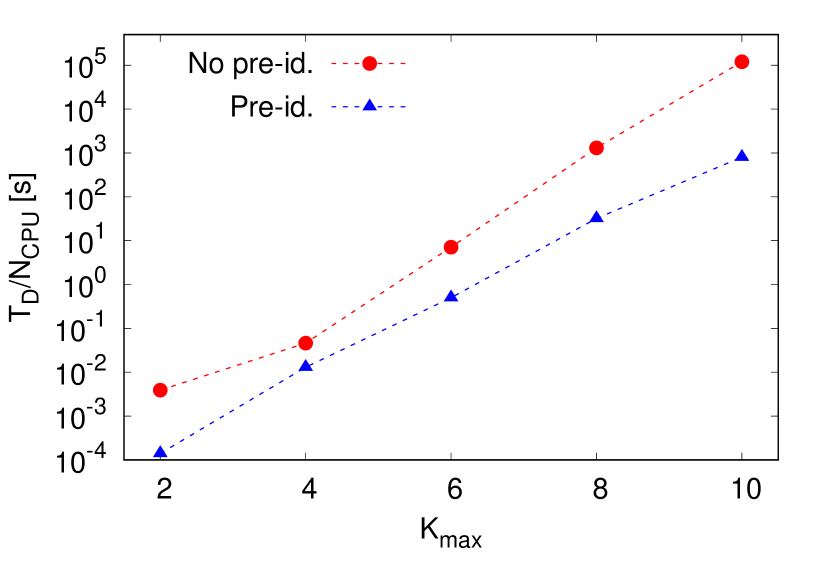
Figure 7: Total time needed to compute the $D$ coefficients [Eq. (93)] as function of $K=K^{\prime}=K_{max}$ divided by $N_{CPU}$, the number of CPUs used in the computation. These calculations are performed for fixed values of the other quantum numbers, in particular $L=L^{\prime}=0$, $S=S^{\prime}=1$ and $T=T^{\prime}=0$. The red dots are the time spent without pre-identification, while the blue triangles are the time spent with pre-identification. The dashed lines are added to guide the eyes. The calculations were performed on a single node with 48 Intel Xenon 8160 CPUs @ 2.10 GHz (i.e. $N_{CPU}=48$).

In Figure 7 we report the total time needed to compute the $D$ coefficients when $L=L^{\prime}=0$, $S=S^{\prime}=1$ and $T=T^{\prime}=0$ up to given $K=K^{\prime}=K_{max}$, namely

$$T_{D}=\sum_{K=2}^{K_{max}}\sum_{K^{\prime}=2}^{K_{max}}T_{op}^{K010,K^{\prime}010}\,.$$ (93)

divided by the number of CPUs ($N_{CPU}$) used in the computation. In particular, the blue triangles give $T_{D}$ by using first the pre-identification of the pair of states $\nu,\nu^{\prime}$ to fulfill the $\delta_{\nu_{x},\nu_{x}^{\prime}}$ condition as discussed before, while the red dots correspond to the time spent without pre-identification. As it is clear from the figure, the computational time increases exponentially by increasing the values of $K_{max}$, since it is proportional to the number of independent states which grows exponentially as well. However, by using the pre-identification, not only $T_{D}$ results to be well reduced, but also as function of $K_{max}$ it has a minor slope compared to the case without pre-identification. The exponential growth limits the maximum value of $K_{max}$ we can use at present. However, we expect to have a great improvement by using a larger number of CPUs distributing the calculation on several nodes.

As regarding the storage, the total memory required for fixed $\gamma$ and $\gamma^{\prime}$ is given by the number of $D$ coefficients for each $\alpha,\alpha^{\prime}$ combination, namely

$$M_{\gamma,\gamma^{\prime}}[{\rm GB}]\sim 3\times\frac{8\times N_{\gamma}\times N_{\gamma^{\prime}}\times N_{V}}{1024^{3}}\,,$$ (94)

where the factor $3$ is an empirical factor, which takes care of the additional information needed in the files to save the coefficients $D$. For example, when $\gamma=\gamma^{\prime}=\{12,2,1,0\}$, the size of the file is only 2.2 GB. The total memory we used to store all the $D$ coefficients used for computing the ${}^{6}{\rm Li}$ ground state in this work is $\sim 100$ GB.

Once computed the $D$ coefficients, the time required for the calculation of all the potential matrix elements is of the order of a couple of hours. Indeed we need only to compute the sum over the combinations $\nu_{y},\nu_{y}^{\prime}$ allowed by the potential ($N_{V}$), which are very few for all the possible $\gamma,\gamma^{\prime}$ and $l,l^{\prime}$. This process can be even accelerated by computing and storing the matrix element of Eq. (LABEL:eq:mxpint) before combining them with the $D$ coefficients.

Typically, in the ab-initio methods, the potential matrix elements are computed and stored for each potential model. By using our approach, we are able to save only the $D$ coefficients by eliminating the dependence on the potential models.

References

- Carlson et al. (2015) J. Carlson, S. Gandolfi, F. Pederiva, S. C. Pieper, R. Schiavilla, K. E. Schmidt, and R. B. Wiringa, Rev. Mod. Phys. 87, 1067 (2015).
- Piarulli et al. (2018) M. Piarulli, A. Baroni, L. Girlanda, A. Kievsky, A. Lovato, E. Lusk, L. E. Marcucci, S. C. Pieper, R. Schiavilla, M. Viviani, and R. B. Wiringa, Phys. Rev. Lett. 120, 052503 (2018).
- Bogner et al. (2007) S. Bogner, R. Furnstahl, and R. Perry, Phys. Rev. C 75, 061001 (2007).
- Jurgenson et al. (2009) E. D. Jurgenson, P. Navrátil, and R. J. Furnstahl, Phys. Rev. Lett. 103, 082501 (2009).
- Barrett et al. (2013) B. R. Barrett, P. Navrátil, and J. P. Vary, Prog. Part. Nucl. Phys. 69, 131 (2013).
- Barnea et al. (2000) N. Barnea, W. Leidemann, and G. Orlandini, Phys. Rev. C 61, 054001 (2000).
- Barnea et al. (2010) N. Barnea, W. Leidemann, and G. Orlandini, Phys. Rev. C 81, 064001 (2010).
- Vaintraub et al. (2009) S. Vaintraub, N. Barnea, and D. Gazit, Phys. Rev. C 79, 065501 (2009).
- Gattobigio et al. (2011) M. Gattobigio, A. Kievsky, and M. Viviani, Phys. Rev. C 83, 024001 (2011).
- Shirokov et al. (2007) A. Shirokov, J. Vary, A. Mazur, and T. Weber, Physics Letters B 644, 33 (2007).
- Volkov (1965) A. Volkov, Nucl. Phys. 74, 33 (1965).
- Varga and Suzuki (1995) K. Varga and Y. Suzuki, Phys. Rev. C 52, 2885 (1995).
- Lazauskas (2019) J. Lazauskas, R. Carbonell, Few-Body System 60, 62 (2019).
- Lazauskas and Carbonell (2020) R. Lazauskas and J. Carbonell, Front. Phys. 7, 251 (2020).
- Kievsky et al. (2008) A. Kievsky, S. Rosati, M. Viviani, L. Marcucci, and L. Girlanda, J. Phys. G: Nucl. Part. Phys. 35, 063101 (2008).
- Marcucci et al. (2020) L. E. Marcucci, J. Dohet-Eraly, L. Girlanda, A. Gnech, A. Kievsky, and M. Viviani, Front. Phys. 8, 69 (2020).
- Efros (1972) V. Efros, Sov. J. Nucl. Phys. 15, 128 (1972).
- Efros (1979) V. Efros, Sov. J. Nucl. Phys. 27, 448 (1979).
- Demin (1977) V. Demin, Sov. J. Nucl. Phys. 26, 379 (1977).
- de la Ripelle (1983) M. F. de la Ripelle, Ann. Phys. 147, 281 (1983).
- Viviani et al. (2005) M. Viviani, A. Kievsky, and S. Rosati, Phys. Rev. C 71, 024006 (2005).
- Viviani (1998) M. Viviani, Few-Body Syst. 25, 177 (1998).
- Dohet-Eraly and Viviani (2019) J. Dohet-Eraly and M. Viviani, (2019), arXiv:1909.00783 [physics.comp-ph] .
- Zernike and Brinkman (1935) F. Zernike and H. Brinkman, Proc. Kon. Ned. Acad. Wensch. 33, 3 (1935).
- Abramowitz and Stegun (1970) M. Abramowitz and I. Stegun, Handbook of Mathematical Functions (Dover Publications, Inc., New York, 1970).
- Cullum and Willoughby (1981) J. Cullum and R. Willoughby, J. Comp. Phys. 44, 329 (1981).
- Entem and Machleidt (2003) D. Entem and R. Machleidt, Phys. Rev. C 68, 041001 (2003).
- Zakharyev and Efros (1969) V. Zakharyev, B.N. Pustovalov and E. Efros, Sov. J. Nucl. Phys. 8, 234 (1969).
- Schneider (1972) T. Schneider, Phys. Lett. B 40, 439 (1972).
- Jurgenson et al. (2011) E. Jurgenson, P. Navrátil, and R. Furnstahl, Phys. Rev. C 83, 034301 (2011).
- Stetcu et al. (2005) I. Stetcu, B. Barrett, P. Navrátil, and J. Vary, Phys. Rev. C 71, 044325 (2005).
- Friar et al. (1997) J. Friar, J. Martorell, and D. Sprung, Phys. Rev. A 56, 4579 (1997).
- Foldy and Wouthuysen (1950) L. Foldy and S. Wouthuysen, Phys. Rev. 78, 29 (1950).
- Tanabashi and et al. (2018) M. Tanabashi and et al. (Particle Data Group), Phys. Rev. D 98, 030001 (2018).
- Puchalski and Pachucki (2013) M. Puchalski and K. Pachucki, Phys. Rev. Lett. 111, 243001 (2013).
- Stone (2014) N. Stone, Table of nuclear magnetic dipole and electric quadrupole moments (IAEA, 2014) and refernces therein.
- Carlson and Schiavilla (1998) J. Carlson and R. Schiavilla, Rev. Mod. Phys. 70, 743 (1998).
- Schiavilla et al. (2019) R. Schiavilla, A. Baroni, S. Pastore, M. Piarulli, L. Girlanda, A. Kievsky, A. Lovato, L. Marcucci, S. C. Pieper, M. Viviani, and R. Wiringa, Phys. Rev. C 99, 034005 (2019).
- Forest et al. (1996) J. Forest, V. Pandharipande, S. Pieper, R. Wiringa, R. Schiavilla, and A. Arriaga, Phys. Rev. C 54, 646 (1996).
- Nollett et al. (2001) K. Nollett, R. Wiringa, and R. Schiavilla, Phys. Rev. C 63, 024003 (2001).
- Navrátil (2004) P. Navrátil, Phys. Rev. C 70, 054324 (2004).
- Navrátil and Quaglioni (2011) P. Navrátil and S. Quaglioni, Phys. Rev. C 83, 044609 (2011).
- Hupin et al. (2015) G. Hupin, S. Quaglioni, and P. Navrátil, Phys. Rev. Lett. 114, 212502 (2015).
- George and Knutson (1999) E. George and L. Knutson, Phys. Rev. C 59, 598 (1999).
- Robertson et al. (1981) R. Robertson, P. Dyer, R. Warner, R. Melin, T. Bowles, A. McDonald, G. Ball, W. Davies, and E. Earle, Phys. Rev. Lett. 47, 1867 (1981).
- Machleidt (2001) R. Machleidt, Phys. Rev. C 63, 024001 (2001).
- Timofeyuk (1998) N. Timofeyuk, Nucl. Phys. A 632, 19 (1998).
- Wiringa et al. (1995) R. B. Wiringa, V. G. J. Stoks, and R. Schiavilla, Phys. Rev. C 51, 38 (1995).
- Pudliner et al. (1997) B. S. Pudliner, V. R. Pandharipande, J. Carlson, S. C. Pieper, and R. B. Wiringa, Phys. Rev. C 56, 1720 (1997).
- Abdelhameed et al. (2019) A. H. Abdelhameed, G. Angloher, P. Bauer, A. Bento, E. Bertoldo, C. Bucci, L. Canonica, A. D’Addabbo, X. Defay, and et al., Eur. Phys. J. C 79 (2019).
- Lewin and Smith (1996) J. Lewin and P. Smith, Astr. Phys. 6, 87 (1996).
- Körber et al. (2017) C. Körber, A. Nogga, and J. de Vries, Phys. Rev. C 96, 035805 (2017).