Non-Kolmogorov scaling for two-particle relative velocity
in two-dimensional inverse energy-cascade turbulence

Abstract

Herein, we numerically examine the relative dispersion of Lagrangian particle pairs in two-dimensional inverse energy-cascade turbulence. Behind the Richardson–Obukhov $t^{3}$ law of relative separation, we discover that the second-order moment of the relative velocity have a temporal scaling exponent different from the prediction based on the Kolmogorov’s phenomenology. The results also indicate that time evolution of the probability distribution function of the relative velocity is self-similar. The findings are obtained by enforcing the Richardson–Obukhov law either by considering a special initial separation or by conditional sampling. In particular, we demonstrate that the conditional sampling removes the initial-separation dependence of the statistics of the separation and relative velocity. Furthermore, we demonstrate that the conditional statistics are robust with respect to the change in the parameters involved, and that the number of the removed pairs from the sampling decreases when the Reynolds number increases. We also discuss the insights gained as a result of conditional sampling.

I Introduction

Relative dispersion has been widely investigated following a pioneering study by Richardson Richardson (1926), who observed the super-diffusive manner of separation between two particles in the atmosphere. The study introduced the diffusion-type differential equation for the probability distribution function (PDF) of separation, $r$. A significant part of this equation is that it includes the diffusion coefficient dependent on $r$ itself. Furthermore, Richardson predicted the celebrated $t^{3}$ law of the second-order moment of the relative separation from the PDF, $\langle r^{2}(t)\rangle\propto t^{3}$, and this is referred to as the Richardson–Obukhov law. The scaling argument leading to this law (which was developed first for the three dimensional (3D) turbulence) can be applicable to two-dimensional (2D) turbulence, as reviewed in Salazar and Collins (2009). In this study, we restrict our attention to the relative dispersion in 2D turbulence.

The $t^{3}$ prediction was performed prior to Kolmogorov’s phenomenology for 3D turbulence proposed in 1941 (K41) Kolmogorov (1941), and later demonstrated as consistent with the K41 dimensional analysis Obukhov (1941); Batchelor (1950). With respect to the 2D turbulence, specifically, in the inverse energy-cascade state, the Richardson–Obukhov law was similarly derived from a 2D analog of the K41, which was developed by Kraichnan, Leith, and Batchelor Kraichnan (1967); Leith (1968); Batchelor (1969); hereinafter, the analog is referred to as K41 for convenience. Specifically, based on the phenomenologies, the second-order moment of the relative separation in the inertial range can assume the following form:

$$\langle r^{2}(t)\rangle\simeq\begin{cases}\langle r_{0}^{2}\rangle+S_{2}(r_{0})t^{2}&(t\ll t_{\mathrm{B}}),\\ g\varepsilon t^{3}&(t_{\mathrm{B}}\ll t\ll T_{L}),\end{cases}$$ (1)

where $r_{0}\equiv|\bm{r}_{0}|$ denotes the initial separation of the pairs, $\varepsilon$ denotes the energy dissipation rate or the energy flux in the inertial range, $S_{2}(r)=C_{2}\varepsilon^{2/3}r^{2/3}$ denotes the second-order longitudinal velocity structure function, $C_{2}$ is a constant, $t_{\mathrm{B}}=r_{0}^{2/3}\varepsilon^{-1/3}$ denotes the Batchelor time, $T_{L}$ denotes the integral time scale, and $g$ denotes the Richardson constant. Up to the Batchelor time $t_{\mathrm{B}}$, each particle moves with the initial velocity. Subsequently, the relative separation becomes independent of $r_{0}$ and behaves according to the $t^{3}$ law, exhibiting super-diffusivity (Richardson–Obukhov regime).

With respect to 2D inverse energy-cascade turbulence, the $t^{3}$ law is observed in laboratory experiments Jullien et al. (1999); von Kameke et al. (2011) for appropriately selected initial separations. Recently, Rivera and Ecke Rivera and Ecke (2005, 2016) performed experiments by varying initial separations and observed that the power-law exponent of $\langle r^{2}(t)\rangle$ in the inertial range depends on the initial separation $r_{0}$. They also observed $t^{3}$-scaling behavior similar to the Richardson–Obukhov scaling law only for a certain range of initial separations. The initial separation dependence and existence of special initial separations leading to the $t^{3}$ law were observed in 2D direct numerical simulation (DNS) Boffetta and Sokolov (2002) as well. With respect to the 3D direct energy-cascade turbulence, the situation is similar: the slope of $\langle r^{2}(t)\rangle$ as a function of $t$ varies due to the length of initial separations in laboratory experiments Ott and Mann (2000). Recently, DNSs in 3D also indicated that the $t^{3}$ law only appears for a certain selected initial separation Yeung and Borgas (2004); Sawford et al. (2008); Bitane et al. (2013).

Based on 2D and 3D results, the conclusion at currently achievable Reynolds numbers is that the time evolution of $\langle r^{2}(t)\rangle$ strongly depends on the initial separation. Thus, the Richardson–Obukhov $t^{3}$ law emerges only for a selected initial separation, and this is termed as the proper initial separation in the current study (as detailed in Sec. III.1). The problem to be solved is the dependence of the $t^{3}$ law on the initial separation; specifically, whether the $t^{3}$ law observed for the special initial separation is relevant with the K41 or just coincidental. It is known that the initial separation dependence is alleviated by considering $\langle|\bm{r}-\bm{r_{0}}|^{2}\rangle$ instead of $\langle r^{2}\rangle$. By analyzing $\langle|\bm{r}-\bm{r_{0}}|^{2}\rangle$ at sufficiently high Reynolds numbers, Bitane et al. Bitane et al. (2012, 2013) introduced the modified scaling law including a subleading term, $\langle|\bm{r}(t)-\bm{r}_{0}|^{2}\rangle=g\varepsilon t^{3}(1+Ct_{0}/t)$ for $t\gg t_{0}$, where $t_{0}$ denotes a time scale of convergence to Richardson–Obukhov regime, $t_{0}=S_{2}(r_{0})/2\varepsilon$, and $C$ denotes a parameter based on $r_{0}$. It is noted that $C=0$ for $r_{0}=4\eta$, where $\eta$ denotes the Kolmogorov length scale. The $r_{0}=4\eta$ is termed as ”optimal choice” in their study and can correspond to the proper initial separation. Furthermore, Buaria et al. Buaria et al. (2015) suggested an asymptotic state, and this is independent of the initial separations. The same authors Buaria et al. (2016) investigated turbulent relative dispersion utilizing diffusing/Brownian particles, i.e., particles of various Schmidt numbers ($Sc$) with white/Brownian noise added to their trajectories. They found that the initial separation dependence is weaker and Richardson scaling is more robust for $Sc=O(1)$ than $Sc=\infty$ (fluid particles).

Several studies Boffetta and Sokolov (2002); Rivera and Ecke (2005) in the 2D inverse-energy cascade turbulence discussed the proper initial separation, and concluded that the $t^{3}$-scaling behavior observed only for the special initial separation is an artifact caused by the finite-size effect of the limited inertial range. Given the aforementioned reasons, they argued that proper initial separation exists even in the low Reynolds-number simulations and that the proper initial separation is significantly lower than the smallest lower bound of the inertial range. In particular, the observed scaling law $\langle r(t)^{2}\rangle\propto t^{3}$ started to hold outside of the inertial range, as already noted in Kellay and Goldburg (2002). Subsequently, the $t^{3}$ law with the proper initial separation extends into the inertial range. However, details of the finite-size effects, e.g., the dependence of the $t^{3}$ law on the width of the inertial range, remains to be clarified.

There is another problem with respect to the proper initial separation. The K41 can be applied to the two-particle Lagrangian relative velocity, and predicts $t^{1}$ scaling for the second-order moment as

$$\langle v^{2}(t)\rangle\propto\varepsilon t^{1},$$ (2)

in the inertial range, where $v(t)$ denotes the relative velocity. In recent 3D numerical studies Yeung and Borgas (2004); Bitane et al. (2013), the relative velocity is also observed to depend on the initial separation such as relative separation. Furthermore, it appears that the second-order moment of the relative velocity exhibits a different scaling exponent from the K41 prediction.

The long-standing problem of two-particle relative diffusion in turbulence can be the applicability of the K41 to the Lagrangian relative separation and velocity statistics and at least at presently available Reynolds numbers. It is well-known that the K41 scaling does not precisely hold, particularly for the 3D turbulence due to the intermittency effect. However, the deviation from the K41 is small with respect to the low-order statistics of the Eulerian velocity such as the energy spectrum or the second-order structure functions. Thus, the K41 is successful for the Eulerian velocity. In contrast, the K41 appears to fail in describing the second-order moments of the relative separation and velocity, which are Lagrangian quantities, to the same extent as the low-order Eulerian velocity. This large gap between Eulerian and Lagrangian statistics should be filled. It is possible that the gap is caused by a finite Reynolds-number effect.

In this study, we numerically examine two-particle relative diffusion in 2D energy inverse-cascade turbulence with either normal viscosity or hyperviscosity. The main reason for selecting the 2D system is that detailed numerical studies (e.g., a large number of particle-pair samples and long-time integration) are more feasible. Furthermore, the Eulerian velocity is intermittency free Paret and Tabeling (1997); Boffetta et al. (2000), and consequently, corresponds to “an ideal framework to examine Richardson scaling in Kolmogorov turbulence”, as noted by Boffetta and Sokolov (2002). Thus, we can factor out the intermittency effect on the deviation of the Lagrangian statistics from the K41 prediction when we analyze 2D results. Evidently, limitations exist while selecting the 2D system. As aforementioned, there are common problems in the Richardson–Obukhov law in 2D and 3D systems. However, their nature is not necessarily identical. Careful discussion and further investigations are required while applying our results in this study to the 3D case. Nevertheless, insights obtained here in 2D can be useful in addressing the 3D problem.

We conduct our numerical study as follows. First, we develop a conditional sampling to remove the initial-separation dependence. We demonstrate that the conditioned $\langle r^{2}(t)\rangle$ curves of various initial separations collapse on the unconditioned curve starting from the proper initial separation. From the robustness, we infer that the $t^{3}$ law of the proper initial separation is consistent with the K41. We then discuss the generality of the conditional sampling, namely, the dependence of the conditioned results on the parameters of the conditional sampling. Finally, we examine the scaling behavior of the relative velocity with and without the conditional sampling in detail.

The two main results obtained in 2D energy inverse-cascade turbulence are: (i) relative velocity deviates from the K41 scaling ,i.e., scaling law (2), although the relative separation obeys the Richardson–Obukhov $t^{3}$ law; and (ii) relative velocity is self-similar (intermittency free).

Both suggest that the K41 does not hold for second-order statistics of relative velocity.

Sec. II presents the details of our 2D numerical study. Sec. III.1 introduces a working hypothesis and describes the proper initial separation. In Sec. III.2, we describe our conditional sampling and discuss what can be inferred from conditional statistics on the relative separation. Sec. IV presents statistics on the relative velocity with and without conditional sampling.

II Numerical simulation method

$N^{2}$	$\delta x$	$\delta t$	$\nu$	$h$	$\alpha$	$k_{f}$	$\varepsilon_{in}$	$\varepsilon$	$\sigma_{\varepsilon}$	$L$	$u_{\mathrm{rms}}$	$Re_{\alpha}$	$N_{p}^{2}$
$1024^{2}$	$0.006$	$0.002$	$1.8\times 10^{-38}$	8	$35$	$249$	$0.1$	$0.019$	$2.9\times 10^{-4}$	$0.38$	$0.5$	$40$	$2048^{2}$
$2048^{2}$	$0.003$	$0.001$	$4.664\times 10^{-43}$	8	$35$	$496$	$0.1$	$0.019$	$2.9\times 10^{-4}$	$0.37$	$0.5$	$80$	$2048^{2}$
$4096^{2}$	$0.0015$	$0.001$	$1.13\times 10^{-47}$	8	$35$	$997$	$0.1$	$0.018$	$2.6\times 10^{-4}$	$0.36$	$0.5$	$160$	$2048^{2}$
$2048^{2}$	$0.003$	$0.004$	$7.666\times 10^{-6}$	1	$3.005$	$200$	$3.027\times 10^{-4}$	$5.28\times 10^{-5}$	$3.35\times 10^{-5}$	$0.47$	$0.076$	$39$	$2048^{2}$

Table 1: Parameters of numerical simulations: $N^{2}$, $\delta x=2\pi/N$, $\delta t$, $\nu$, $h$, $\alpha$, $k_{f}$, $\varepsilon_{in}$, $\varepsilon$, $\sigma_{\varepsilon}$, $L$, $u_{\mathrm{rms}}$, $Re_{\alpha}$ and $N_{p}^{2}$ denote the number of grid points, grid spacing, size of the time step, (hyper)viscosity coefficient, order of the Laplacian of the (hyper)viscosity, hypodrag coefficient, forcing wavenumber, energy input rate of the forcing, mean of the resultant energy flux in the inertial range, standard deviation of the resultant energy flux, integral scale, root-mean-square velocity, infrared Reynolds number and number of the Lagrangian particles, respectively.

We mainly consider pair-dispersion statistics in a statistically steady, homogeneous, and isotropic 2D inverse-energy cascade turbulent velocity field $\bm{u}(\bm{x},t)$. In the velocity field, we perform a set of DNSs of the 2D incompressible Navier-Stokes equation in a doubly periodic square of side length, $2\pi$. We integrate the equation in the form of vorticity, $\omega(\bm{x},t)=\partial_{x}u_{y}({\bm{x}},t)-\partial_{y}u_{x}({\bm{x}},t)$, which is

$$\frac{\partial\omega}{\partial t}+\left(\bm{u}\cdot\nabla\right)\omega=(-1)^{h+1}\nu\Delta^{h}\omega+\alpha\Delta^{-1}\omega+f.$$ (3)

The setting and our numerical method are identical to those used in Xiao et al. (2009); Mizuta et al. (2013). Here, $\nu$ denotes the (hyper)viscosity coefficient and $\alpha$ denotes the hypodrag coefficient. The order of the Laplacian of the (hyper)viscosity, $h$, is set to $8$ or $1$. The forcing term, $f({\bm{x}},t)$, is given in terms of the Fourier coefficients, $\hat{f}(\bm{k},t)=k^{2}\varepsilon_{in}/[n_{f}\hat{\omega}^{*}(\bm{k},t)]$, where   $\hat{f}$   denotes the Fourier transform of the function $f(\bm{x},t)$. The energy input rate is denoted by $\varepsilon_{in}$, and $n_{f}$ denotes the number of the Fourier modes in the following forcing wavenumber range. We select the coefficients, $\hat{f}({\bm{k}},t)$, as non-zero only in high wave numbers, $\bm{k}$, satisfying $k_{f}-1<|\bm{k}|<k_{f}+1$. Thus, the energy input rate is maintained as constant in time. Numerical integration of Eq. (3) is performed via the pseudospectral method with the 2/3 dealiasing rule in space and the 4-th order Runge–Kutta method in time. Table 1 lists the parameters of simulations used in the study.

In the 2D energy inverse-cascade turbulence, the energy pumped in at the small scale is transported to larger scales with a constant flux on average in the inertial range. To measure this flux, we use the standard method to calculate the energy flux function in the Fourier space. As shown in Fig. 1(a) and (c), the flux becomes wavenumber independent in the intermediate wavenumbers. We consider the range of the wavenumbers as the inertial range. Strictly speaking, a flat region is absent in Fig. 1 (c) due to normal viscosity. The energy flux in the inertial range is equal to the energy dissipation rate taken out by the large-scale hypodrag, $\varepsilon=\int_{0}^{\infty}2\alpha k^{-2}E(k)\mathrm{d}k$, where $E(k)$ denotes the time-averaged energy spectrum. This corresponds to a standard method to numerically realize a statistically steady state of 2D energy inverse-cascade turbulence in a periodic domain. A statistically steady state is judged from behavior of energy as a function of time. The typical wavenumber of the hypodrag is dimensionally estimated as $(\alpha^{3}/\varepsilon)^{1/8}$, which is termed as the frictional wave number, $k_{\alpha}$. Here, we use the infrared Reynolds number, $Re_{\alpha}\equiv k_{f}/k_{\alpha}$, as proposed by Vallgren Vallgren (2011) in order to quantify the span of the inertial range. At the end of Sec. IV, we simulate a statistically quasi-steady state Kraichnan (1967) by solving Eq. (3) without the hypodrag.

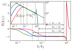
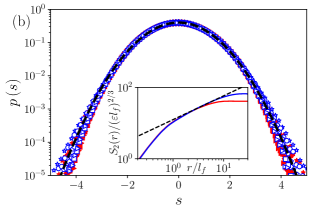
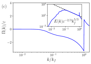
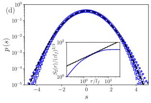
Figure 1: (a) Time-averaged energy flux $\Pi(k)$ for $Re_{\alpha}=40$ (red line), $Re_{\alpha}=80$ (blue line) and $Re_{\alpha}=160$ (green line). Ranges between the two gray dotted lines correspond to the inertial ranges as determined by the plateau regions of the energy flux in the Fourier space. The inset shows the time-averaged energy spectrum $E(k)$ for $Re_{\alpha}=40$ (red line), $Re_{\alpha}=80$ (blue line) and $Re_{\alpha}=160$ (green line). (b) Normalized PDFs of the longitudinal velocity increments for $Re_{\alpha}=40$ (red) and $Re_{\alpha}=80$ (blue) at various separations, $r/l_{f}=1.1,1.5,2.2,3.2,4.8$ and $7.1$. Here, $l_{f}=2\pi/k_{f}$ is the forcing scale and longitudinal velocity increment, $\delta u_{l}$, normalized by the second-order moment and is denoted by $s$: $s=\delta u_{l}/\sqrt{\langle\delta u_{l}^{2}\rangle}$. The dotted line denotes the Gaussian distribution with zero mean and unit variance. The inset shows the second-order longitudinal structure function, $S_{2}(r)$ for $Re_{\alpha}=40$(red) and $Re_{\alpha}=80$(blue). The dashed line represents the K41 scaling, $r^{2/3}$, for $S_{2}(r)$. (c) Same as (a) albeit for the normal viscous case ($h=1$). (d) Same as (b) albeit for the normal viscous case ($h=1$).

Subsequently, we demonstrate that the Eulerian statistics on the velocity field are consistent with the established picture of the 2D inverse energy-cascade turbulence. As shown in the inset of Fig. 1(a) and (c), the energy spectra in the inertial range is consistent with the K41 and more precisely with the Kraichnan-Leith-Batchelor phenomenology. Figures 1(b) and (d) show that the PDFs of the longitudinal velocity increments, $\delta u_{l}(r,t)=[\bm{u}(\bm{x}+\bm{r},t)-\bm{u}(\bm{x},t)]\cdot\bm{r}/r$, at various $r$’s in the inertial range collapse well to the Gaussian distribution irrespective of $r$, and this is in agreement with Boffetta et al. (2000). Here, $l_{f}=2\pi/k_{f}$ denotes the forcing length scale.

To obtain the Lagrangian statistics, we employ a standard particle tracking method. The flow is seeded with a large number of tracer particles, i.e., $N_{p}^{2}$, in the velocity field. The particles are tracked in time via integrating the advection equation,

$$\frac{\mathrm{d}}{\mathrm{d}t}\bm{x}_{p}(t)=\bm{u}(\bm{x}_{p}(t),t),$$ (4)

where $\bm{x}_{p}(t)$ denotes the particle position vector. The numerical integration of Eq. (4) is performed using the Euler method. The velocity value at an off-grid particle position is estimated by the fourth-order Lagrangian interpolation of the velocity calculated on the grid points.

The relative separation, $\bm{r}(t)$, is defined by $\bm{r}(t)=\bm{x}_{1}(t)-\bm{x}_{2}(t)$, where $\bm{x}_{1}$ and $\bm{x}_{2}$ denote the positions of a particle pair. The particles are initially seeded on square grid points where the grid spacing corresponds to $r_{0}$. The statistics on the relative separation are calculated for the nearest neighbor particles at the initial time. In this study, we vary the initial separation $r_{0}$ while maintaining the same total number, $N_{p}^{2}$, of the particles for each $r_{0}$. For small values of $r_{0}$ (which are typically lower than the Eulerian grid size $\delta x$), the initial particles do not cover the whole periodic domain. We verify that the inhomogeneity of the initial positions of the particles does not affect Lagrangian statistics that are examined here by comparing results with different initial particle positions covering different parts of the periodic domain. In addition to the separation, $r(t)$, our focus is on the longitudinal relative velocity of particle pairs as defined by $v_{l}(t)\equiv[\bm{u}(\bm{x}_{1}(t),t)-\bm{u}(\bm{x}_{2}(t),t)]\cdot\bm{r}(t)/r(t)$.

We next discuss on how long we track the particles. We continue the tracking until all the particle pairs leave the inertial range. We observe that this time typically concerns $10$ large-scale eddy turn-over times ($L/u_{\rm rms}$) for the hyperviscous $Re_{\alpha}=40$ case and approximately $20$ turn-over times for the hyperviscous $Re_{\alpha}=80$ case. With respect to each $r_{0}$, we perform the simulation of the duration twice.

The largest resolution simulation ($N^{2}=4098^{2}$) as listed in Table 1 is used only for confirming self-similarity of PDF of $v_{l}(t)$ in Sec. IV. We define the Lagrangian average $\langle\cdot\rangle$ as $\langle A\rangle=\frac{1}{N_{\mathrm{adj}}}\sum_{i=1}^{N_{\mathrm{adj}}}A_{i}$, where $A$ denotes any Lagrangian quantity and $A_{i}$ denotes a realization of $A$ by the $i$-th particle pair. $N_{\mathrm{adj}}=2N_{p}(N_{p}-1)$ denotes the number of pairs of particles which adjoin each other at the initial time.

In the following sections, we mainly use hyperviscosity rather than normal viscosity for DNSs. This is because the hyperviscosity extends the inertial range for a given spatial resolution. However, it is known to affect the statistics at the transition between the inertial and dissipation ranges Boffetta and Ecke (2012). Thus, it is possible that the hyperviscosity affects particle-pair statistics. Therefore, we perform hyperviscous and normal-viscous simulations and confirm that the hyperviscosity does not affect the particle-pair statistics.

III Initial separation dependence of relative diffusion statistics and conditional sampling

III.1 Proper initial separation

At the Reynolds numbers currently available in experiments and numerical simulations, the time evolution of $\langle r^{2}(t)\rangle$ depends on the initial separation. Hence, it is not possible to conclude whether it obeys the Richardson–Obukhov prediction $\langle r^{2}(t)\rangle\propto\varepsilon t^{3}$ ( for e.g., Biferale et al. (2005); Bitane et al. (2013) for the 3D case and Jullien et al. (1999); Boffetta and Sokolov (2002) for the 2D inverse energy-cascade case). The same is applicable to the second-order moment of relative velocity, $\langle v^{2}_{l}(t)\rangle$ for which the K41 dimensional analysis yields $\langle v^{2}_{l}(t)\rangle\propto\varepsilon t$ (for e.g., Yeung and Borgas (2004) for the 3D case). In the 2D simulation at moderate Reynolds numbers, the initial-separation dependence is clearly confirmed for both $\langle r^{2}(t)\rangle$ shown in Fig. 2(a) and (c) and $\langle v^{2}_{l}(t)\rangle$ shown in Fig. 2(b) and (d) where $t_{f}=(l_{f}^{2}/\varepsilon)^{1/3}$ denotes the forcing time scale. We examine the results by varying the initial separations below the forcing scale, namely $r_{0}<l_{f}$. Thus, the initial separations are in the scales lower than the inertial range. If we set the initial separation in the inertial range, the graphs of $\langle r^{2}(t)\rangle$ and $\langle v^{2}_{l}(t)\rangle$ are located (they are not shown) above the curves plotted in Fig. 2. Thus, we normalize all quantities by $l_{f}$ and $t_{f}$ unless there is some particular reason. This is because $l_{f}$ and $t_{f}$ approximately define the lowest length and time scale of the inertial range, respectively.

The data with the initial-separation dependence indicates that it is possible to select a special value corresponding to $r_{0}$ for which $\langle r^{2}(t)\rangle$ becomes consistent with the Richardson–Obukhov law $\langle r^{2}(t)\rangle=g\varepsilon t^{3}$. Further, we include the Richardson constant, $g$, which is non-dimensional and possibly universal. We show the squared separation of the special case in the inset of Fig. 2(a) as a logarithmic local slope. However, it should be noted that (even for the special case) agreement of the squared velocity with the K41 prediction, $\langle v_{l}^{2}(t)\rangle\propto\varepsilon t$ is not as good as that of the squared separation. This is observed in the inset of Fig. 2(b).

Given the apparent failures of the K41, in this study, we still argue that a certain bulk of the particle pairs starting from each initial separation $r_{0}$ shown in Fig. 2 obey the Richardson–Obukhov law of the squared separation even at the moderate Reynolds numbers. Thus, we perform conditional sampling of particle pairs. The qualitative condition is that we remove particle pairs that prevent from separating too fast. In the following section, we demonstrate that this type of a conditional average $\langle r^{2}(t)\rangle_{c}$ becomes independent of the initial separation and that $\langle r^{2}(t)\rangle_{c}$ is the same as the unconditioned $\langle r^{2}(t)\rangle$ commencing from the special initial separation (see Fig. 4). Hence, the conditional sampling recovers the Richardson-Obukhov law, $\langle r^{2}(t)\rangle_{c}=g\varepsilon t^{3}$, including the Richardson constant and flux. Thus, we term the special initial separation as the proper initial separation, which we denote as $r_{0}^{(p)}$

Evidently, our conditional sampling is contrived. It has several tuning parameters as we will specify them. We determine their values empirically by ensuring that $\langle r^{2}(t)\rangle_{c}\propto t^{3}$ holds. In order to demonstrate the extent to which it is contrived, we examine the manner in which conditional statistics change by varying tuning parameters. Furthermore, we demonstrate that the number of removed pairs decreases when the Reynolds number increases. The details of the conditional sampling are given in the next subsection.

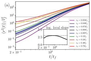
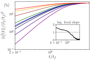
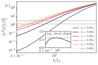
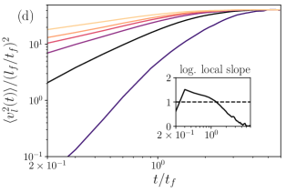
Figure 2: (a) Mean squared separation for the hyperviscous case with $Re_{\alpha}=40$ as a function of time for various initial separations. Here, $t_{f}=(l_{f}^{2}/\varepsilon)^{1/3}$ denotes the forcing time scale. The ranges between the two horizontal lines correspond to the inertial range determined by the region of the mean exit time that is proportional to $r^{2/3}$, which is discussed later. Inset: the logarithmic local slope for the special initial separation, $r_{0}=0.088l_{f}\sim r_{0}^{(p)}$, where $\varepsilon$ denotes the mean energy flux in the inertial range. The gray dashed line corresponds to the Richardson scaling exponent, $3$. (b) mean squared relative velocity for various initial separations. Inset: the logarithmic local slope for the special initial separation, $r_{0}=0.088l_{f}$. The gray dashed line corresponds to the Kolmogorov scaling exponent, $1$. (c) Same as (a) albeit for the normal viscous case. (d) Same as (b) albeit for the normal viscous case.

III.2 Conditional sampling via mean exit time

Figure 2(a) plots nine cases of the different initial separations. To develop the conditional sampling, we first focus on initial separations that satisfy $r_{0}>r_{0}^{(p)}$, where $r_{0}^{(p)}$ denotes the proper initial separation. Thus, we consider three cases from above in In Fig. 2(a). Our estimate of the proper initial separation is empirical: we examine the compensated plot of the unconditional moment $\langle r^{2}(t)\rangle$ as shown in Fig. 2(a) by changing $r_{0}$. Subsequently, we select $r_{0}$ for which the compensated plot exhibits the widest plateau. We evaluate the proper initial separation in this manner as $r_{0}^{(p)}=0.088l_{f},0.101l_{f}$, and $0.121l_{f}$ for $Re_{\alpha}=40,80$, and $160$, respectively.

With respect to the initial separations $r_{0}>r_{0}^{(p)}$, the graphs of the mean squared separation $\langle r^{2}(t)\rangle$ are situated above the graph starting from $r_{0}^{(p)}$ as shown in Fig. 2. This indicates that it is necessary to remove particle pairs that separate too fast to recover the $t^{3}$ scaling. Now, we pose two questions on the conditional sampling: (A) Is it possible to instantaneously determine whether it is excessively fast, i.e., exhibiting excessively large $r(t)$?; (B) How to draw a line between excessively fast pairs and not excessively fast pairs, i.e., the threshold level between the two sets? We handle both the questions with exit-time statistics that are proved as effective tools in the study of relative diffusion.

The exit time concerns the first passage time. The first passage time of the separation $r(t)$ for a given value $R$ is defined by the first instance when the separation $r(t)$ becomes equal to $R$. (for the first passage time of a general stochastic process, see, e.g., Gardiner (2009)). We express the first passage time as $T_{F}(R)$. To define the exit time, it is necessary to set the domains. We denotes the domain as a series $R_{0},R_{1},R_{2},\ldots$. The exit time of the $j$-th zone $R_{j-1}\leq r(t)<R_{j}$ is then defined as $T^{(j)}_{E}=T_{F}(R_{j})-T_{F}(R_{j-1})$ where $R_{j}=r_{s}\rho^{j}$ with parameters $r_{s}$ and $\rho>1$ for $j=1,2,\ldots$. In the relative diffusion problem, exit-time statistics are introduced to solve the finite-size problems Artale et al. (1997); Boffetta et al. (1999); Boffetta and Sokolov (2002); Rivera and Ecke (2005). By selecting thresholds $R_{j}$s in the inertial range, it is possible to exclusively extract information of the inertial range. It is known that exit-time statistics are insensitive to the Reynolds number(for e.g.,Ogasawara and Toh (2006a)). It is also known that the mean exit time is consistent with the K41 prediction, $\langle T^{(j)}_{E}\rangle\propto R_{j}^{2/3}$ when $R_{j}$ is in the inertial range. Furthermore, the scaling behavior holds independent of the initial separations Boffetta and Sokolov (2002); Biferale et al. (2005). In our simulation with $r_{s}=1.3l_{f}$ and $\rho=1.1$, the K41 scaling of the mean exit time is observed for $1\leq j\leq 7$ for the hyperviscous $Re_{\alpha}=40$ case and $1\leq j\leq 14$ for the hyperviscous $Re_{\alpha}=80$ case as shown in Fig. 3. Typical value of $\rho$ as used in the previous studies corresponded to $1.1$ or $1.2$ Artale et al. (1997); Boffetta et al. (1999); Boffetta and Sokolov (2002); Rivera and Ecke (2005); Ogasawara and Toh (2006a) and the properties of exit-time statistics as mentioned above do not change in the range of $\rho$.

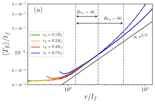
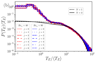
Figure 3: (a) Mean exit time for the hyperviscous cases with $Re_{\alpha}=40$ (dash-dotted line) and $Re_{\alpha}=80$ (solid line). Black solid line denotes $r^{2/3}$ power law. The ranges between the two gray dashed lines denote the inertial range estimated with the exit time at $Re_{\alpha}=40$ and $Re_{\alpha}=80$. (b) The PDFs of exit time normalized by the mean at $Re_{\alpha}=40$ (red) and $80$ (blue) for $j=0$ to $6$. Black dashed line and solid line denote longtime asymptotic forms for the PDF of exit times, i.e., $P(T_{E})\langle T_{E}\rangle\sim C\sum_{i=1}^{N}j_{2,i}J_{2}^{\prime}(j_{2,i})\exp[-\frac{j_{2,i}^{2}}{12}\frac{\rho^{2/3}-1}{\rho^{2/3}}\frac{t}{\langle T_{E}\rangle}]$ Boffetta and Sokolov (2002), at $N=1$ and $N=3$, respectively. Here, $C$ denotes the normalized factor, $J_{2}$ denotes the Bessel function, and $j_{2,i}$ denotes the $i$-th zero point of $J_{2}$ and $\rho=1.1$.

Now, we describe how we address the two questions of conditional sampling with the exit time. For the first question (A), we assume that it is not possible to instantaneously determine excessively-fast pairs. This is performed over certain consecutive zones in the inertial range. We express the number of the zones by $N_{Q}$ (at the end of Sec. III.2. We change the parameter $N_{Q}$ and discuss question (A).).

With respect to the second question (B), evidently small exit time $T_{E}^{(j)}$ corresponds to pairs separating fast. Hence, to remove the excessively-fast pairs, we set an upper threshold, $\tau$, in terms of the exit time over the zones $j=1,2,\ldots,N_{Q}$. Hence, if the exit time of the particle pair satisfies

$$\frac{T_{E}^{(j)}}{\langle T_{E}^{(j)}\rangle}\leq\tau$$ (5)

in all of the zones, $j=1,2,\ldots,N_{Q}$, then this type of a pair is removed from the Lagrangian average. It should be noted that the threshold $\tau$ is independent of $j$. The condition implies that the removed pairs spend a short time when compared to the average in any of the $N_{Q}$ zones. Thus, the removed pair separate too fast in all of the monitored zones. Conversely, the remaining pairs in the conditional sampling generally spend a sufficiently long time such that $T_{E}^{(j)}/\langle T_{E}^{(j)}\rangle>\tau$. However, they can become excessively-fast in several (but not all) of the $N_{Q}$ zones. It should be noted that the conditional sampling includes two parameters: $N_{Q}$ and $\tau$.

Our physical picture of the conditional sampling is as follows: The pair separation $r(t)$ is given by the time integral of the relative velocity from time $0$ to $t$. The accumulating nature of $r(t)$ suggests that it is necessary to consider the history of a pair in conditional sampling. We consider it in terms of the $N_{Q}$ zones starting from the lowest scale of the inertial range. An actual value of $N_{Q}$ will be determined empirically. With respect to $\tau$, it is noted that the right part of the PDF of the exit time is given by the Richardson PDF of the separation, $P(r,t)\propto\varepsilon^{-1}t^{-3}\exp[-({\rm const.})\varepsilon^{-1/3}t^{-1}r^{2/3}]$, which denotes the self-similar solution to the Richardson’s diffusion (Fokker-Plank) equation Boffetta and Sokolov (2002). The correspondence of the PDFs shown in Fig. 3(b) indicates that the pairs in the left part in the exit-time PDF should be removed in the conditional sampling, thereby leading to the criterion, Eq. (5). This picture is only qualitative in nature.

We then describe the determination of parameter values in practice. In the case of $Re_{\alpha}=40$, the inertial range is covered by $7$ zones. Hence, we set the number of the monitored zones to $N_{Q}=7$. Subsequently, we tune the threshold $\tau$’s based on the initial separation $r_{0}$ to recover the Richardson–Obukhov law by examining whether the compensated plot $\langle r^{2}(t)\rangle_{c}/(\varepsilon t^{3})$ exhibits a plateau. We empirically determine that the $\tau$ values correspond to $0.40,1.2,3.4$, and $4.6$ for the initial separations $r_{0}/l_{f}=0.12,0.24,0.48$, and $0.71$, respectively. Given the parameters, we present the results of the conditional average of the squared separations in Fig. 4(a). With respect to the hyperviscous $Re_{\alpha}=80$ case, the inertial range is covered by $14$ zones. However, we demonstrate the result with the same $N_{Q}=7$ as that in the lower Reynolds number case to enable a better comparison in Fig. 4(b).

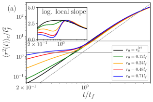
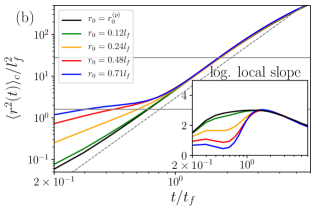
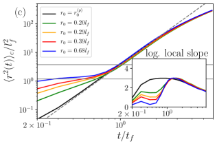
Figure 4: Conditionally sampled second-order moments of relative separations. The initial separations exceed the proper initial separation $r_{0}^{(p)}$. (a) Conditional sampling for the hyperviscous $Re_{\alpha}=40$ case starting from various initial separations. (b) Conditional sampling for the hyperviscous $Re_{\alpha}=80$ starting from various initial separations. (c) Conditional sampling for the viscous $Re_{\alpha}=39$ case starting from various initial separations. Inset shows the logarithmic local slopes of the conditionally sampled $\langle r^{2}(t)\rangle$. Black solid curve shows the second-order moment of the relative separation without any conditional sampling starting from the proper initial separation, $r_{0}=r_{0}^{(p)}$. The gray dashed line denotes $t^{3}$ power law. The range between the two horizontal gray solid lines denotes the inertial range estimated with the exit time.

The thresholds are observed as $\tau=0.25,0.50,1.4$ and $3.0$ for the same set of the initial separations $r_{0}/l_{f}=0.12,0.24,0.48$ and $0.71$, respectively. In the normal-viscous case, $N_{Q}=7$ and the thresholds correspond to $\tau=0.45,1.05,2.4$, and $4.4$ for the initial separations $r_{0}/l_{f}=0.20,0.29,0.39$ and $0.68$, respectively.

As shown in Fig. 4, the conditioned curves $\langle r^{2}(t)\rangle_{c}$ collapse in the inertial range and beyond the unconditioned curve for proper initial separation. It should be noted that the width of the collapsed region increases as we increase $Re_{\alpha}$. When we compare $\tau$ between the two Reynolds number cases for the same normalized initial separation $r_{0}/l_{f}$, it approximately decreases by a factor of $1/2$. The fraction of the remaining pairs in the conditional sampling corresponds to $41$ % for $Re_{\alpha}=40$ and $65$ % for $Re_{\alpha}=80$. Qualitatively, the increase in the fraction is interpreted as follows. We assume that we compare each pair’s distance $r(t)$ at the same time $t$ for the two Reynolds numbers. Given the wider inertial range at higher $Re_{\alpha}$, pairs with larger separation $r(t)$ (i.e., pairs separating fast) are tolerated in the higher $Re_{\alpha}$ case to recover the Richardson–Obukhov law. The increase in the fraction supports the working hypothesis that a certain bulk of particle pairs obey the Richardson–Obukhov law even at moderate Reynolds numbers.

We then examine changes in the results of the conditional sampling when we vary parameters $N_{Q}$ and $\tau$’s for various initial separation $r_{0}$. For the purpose of simplicity, we limit ourselves to the two hyperviscous cases with $Re_{\alpha}=40$ and $80$. With respect to the reference exit-time statistics, we do not change the parameters $r_{s}=1.30l_{f}$ and $\rho=1.1$. At $Re_{\alpha}=40$, we use $N_{Q}=7$ as the number of monitored zones independent of the initial separation $r_{0}$. The $N_{Q}$ zones, $R_{1}=r_{s}\rho\leq R\leq R_{7}=r_{s}\rho^{7}$, cover almost the entire inertial range. We consider the initial separations satisfying $r_{0}^{(p)}<r_{0}<r_{s}$. We then reduce $N_{Q}$ to $6,5,4,3,2$, and $1$ although we use the same set of $\tau$’s determined with $N_{Q}=7$. The results indicate that further tuning of $\tau$ for the change in $N_{Q}$ is not necessary. The reduction of $N_{Q}$ does not alter the behavior of $\langle r^{2}(t)\rangle_{c}$ as shown in Fig. 4(a). The same is applicable to the higher $Re_{\alpha}=80$ case shown in Fig. 4(b). In this case, we change $N_{Q}$ to $14,13,\dots,1$ although we use the same $\tau$ for each $N_{Q}$. Therefore, the result of the conditional sampling is robust relative to changes in the parameters. An important result obtained in the examination is that $N_{Q}=1$ is sufficient. This answers question (A) on the conditional sampling, namely it is not possible to instantaneously determine if a given pair is excessively fast (consequently exhibiting excessively high $r(t)$). However, it can be performed in terms of the exit time of the first zone in the inertial range. Thus, it is possible to locally remove excessively-fast pairs to recover the Richardson–Obukhov law in space at the entry of the inertial range. Evidently, this is not locally in time. This implies that evolution of a pair in the inertial range is somewhat monotone after the entry. As shown in the next section, this is observed as a self-similar evolution of the relative velocity.

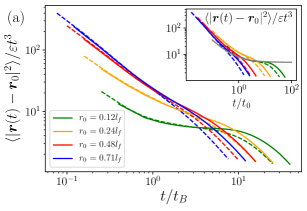
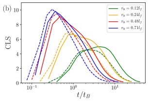
Figure 5: (a) Mean squared separations for the hyperviscous case with $Re_{\alpha}=40$ (dashed line) and $Re_{\alpha}=80$ (solid line), although the initial separation is subtracted for various initial separations. This is compensated by the scaling $\varepsilon t^{3}$. Inset shows the same plots as the main panel although the horizontal axis is compensated by the Bitane time scale, $t_{0}=S_{2}(r_{0})/2\varepsilon$. Gray line denotes the scaling law, $\langle\bm{r}(t)-\bm{r}_{0}\rangle=g\varepsilon t^{3}(1+Ct_{0}/t)$ as suggested by Bitane et al. Bitane et al. (2012). Here, $C=0.6$. (b) Cubed-local slopes of $\langle r^{2}(t)\rangle$ for various initial separations at the hyperviscous $Re_{\alpha}=40$ (dashed line) and $Re_{\alpha}=80$ (solid line). In panel (a) and (b), the time is normalized with the Batchelor time, $t_{\mathrm{B}}=r_{0}^{2/3}\langle\varepsilon\rangle^{-1/3}$. In the inset of panel (a), the time is normalized with Bitane time, $t_{0}=S_{2}(r_{0})/2\varepsilon$.

Other methods are developed to remove the initial separation dependence. For the purpose of comparison, we apply two methods used for 3D turbulence Bitane et al. (2012, 2013); Buaria et al. (2015) to 2D data without utilizing conditional sampling. A method involves subtracting the initial-separation vector ${\bm{r}}_{0}$ from the separation vector ${\bm{r}}(t)$. In Fig. 5 (a), we plot $\langle|{\bm{r}}-{\bm{r}}_{0}|^{2}\rangle/(\varepsilon t^{3})$ of our data for the $Re_{\alpha}=80$ case with the hyperviscosity. The Richardson–Obukhov law appears as a plateau in the region $t/t_{B}\gg 1$ or $t/t_{0}\gg 1$. Although the range of $t/t_{B}$ in our data is comparable to that in the 3D study Buaria et al. (2015), the degree of collapse of our 2D data is worse than that of the 3D result. The other method involves extracting the possibly subdominant $t^{3}$ term in $r(t)$ with a suitable exponentiation and temporal finite difference. In Fig. 5 (b), we plot the cubed local-slope (CLS), $\left\{(d/dt)[\langle r^{2}(t)\rangle^{1/3}]\right\}^{3}/\varepsilon$, Buaria et al. (2015) of our 2D data. The Richardson–Obukhov law appears as a plateau in the CLS in $t/t_{B}\gg 1$. However, the degree of the collapse for the 2D result is worse. The discrepancy between the 2D and 3D cases can be ascribed to the difference in the physics of turbulence in 2D and 3D. Conversely, the plateau is unclear irrespective of the dimensions. This can be due to finite Reynolds number effects. However, in order to evaluate the effects, it is necessary to add the tuning parameter to the Richardson–Obukhov law. A physical meaning of the tuning parameter is obscure in many cases. Although the scaling law suggested by Bitane et al. Bitane et al. (2012) approximately corresponds to data for finite Reynolds number at small time, $t\lesssim t_{0}$, by tuning the parameter, $C$, it does not correspond to the data at large time, $t\gtrsim t_{0}$. Hence, it is necessary to add another tuning parameter for large time. Furthermore, the cause for the difference between $\langle r^{2}(t)\rangle$ and $\langle|{\bm{r}}(t)-{\bm{r}}_{0}|^{2}\rangle$ is not clarified. Hence, it is insufficient to only investigate statistical moments of all particle pairs. Thus, it is necessary to investigate the PDF of particle pairs. We should consider extreme events of particle pairs that can affect even lower moments such as $\langle r^{2}(t)\rangle$. It is intrinsically necessary to consider conditional statistics on a special part of particle pairs.

So far, we restricted the conditional sampling for the cases of $r_{0}>r_{0}^{(p)}$. For lower initial separations, $r_{0}<r_{0}^{(p)}$, we can also recover $t^{3}$ scaling with the same conditional statistics. However, we found that the results indicate the condition for the threshold, $\tau$, changes from the inequality (5) to

$$\tau_{1}\leq\frac{T_{E}^{(j)}}{\langle T_{E}^{(j)}\rangle}\leq\tau_{2},$$ (6)

where $\tau_{1}\not=0$. For example, we empirically determine $(\tau_{1},\tau_{2})=(0.16,7.5),(0.2,1.0)$ and $(0.18,0.50)$ for initial separations $r_{0}/l_{f}=0.024,0.049$, and $0.073$, respectively at $Re_{\alpha}=40$. Although $t^{3}$ scaling law is recovered via conditional sampling, the Richardson constant, $g=\langle r^{2}(t)\rangle_{c}/\varepsilon t^{3}$, for the conditional data is extremely sensitive to the initial separations (figure not shown). The sensitivity considerably differs from the cases of $r_{0}>r_{0}^{(p)}$. This indicates that for $r_{0}<r_{0}^{(p)}$ cases, we fail to construct conditional statistics that remove the initial separation dependence. We infer that in these cases the bulk of particle pairs do not obey the Richardson–Obukhov law in the aforementioned cases. The initial separations are extremely small such that the pairs experience effects from the dissipation range and the small-scale forcing is longer than that of the cases with $r_{0}>r_{0}^{(p)}$. Hence, two parameters are required for conditional sampling. We do not focus on cases with $r_{0}<r_{0}^{(p)}$ in the remaining part of the paper. However, the failure implies that $r_{0}^{(p)}$ corresponds to the border line of the initial separation, beyond which the bulk of the particle pairs becomes consistent with the Richardson–Obukhov law.

IV Scaling of the relative velocity

IV.1 Conditional sampling

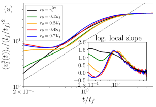
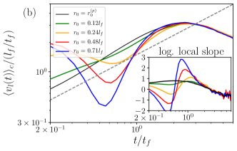
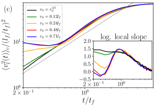
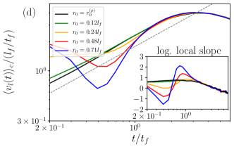
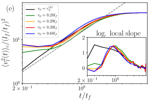
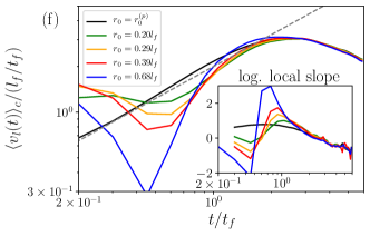
Figure 6: Second-order (left panels) and first-order (right panels) moments of the longitudinal relative velocity for conditionally sampled data starting from various initial separations and for the unconditioned data starting from the proper initial separation, $r_{0}^{(p)}$. Inset: Logarithmic local slope. (a) (b) $Re_{\alpha}=40$ with hyperviscosity. (c) (d) $Re_{\alpha}=80$ with hyperviscosity. (e) (f) $Re_{\alpha}=39$ with normal viscosity. Dashed line denotes $t^{1.23}$ and $t^{0.7}$ scalings for second-order and first-order moments, respectively.

Using the conditional sampling described in the previous section, we show conditional averages of the squared longitudinal relative velocity, $\langle v^{2}_{l}(t)\rangle_{c}$ in Fig. 6. Conditional velocity statistics exhibit a collapse similar to that of the conditional separations. Hence, the second-order and first-order conditional moments, $\langle v^{2}_{l}(t)\rangle_{c}$ and $\langle v_{l}(t)\rangle_{c}$, respectively, starting from various initial separations become almost identical to the unconditioned moments starting from the proper initial separation. However, the degree of collapse of the velocity data is worse at the hyperviscous $Re_{\alpha}=40$ and normal viscous $Re_{\alpha}=39$ although it improves at $Re_{\alpha}=80$ with hyperviscosity. The results indicate that the second-order conditional moment $\langle v^{2}_{l}(t)\rangle_{c}$ and conditional average $\langle v_{l}(t)\rangle_{c}$ deviate from their K41 power-law predictions, $t^{1}$ and $t^{1/2}$, respectively. This contrasts with the conditional relative separation $\langle r^{2}_{l}(t)\rangle_{c}$ that is driven as consistent with the K41 prediction or the Richardson–Obukhov law.

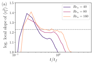
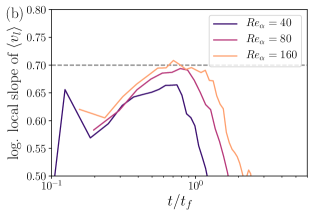
Figure 7: $Re_{\alpha}$-dependence of the logarithmic local slope of (a) $\langle v_{l}^{2}(t)\rangle$, and (b) $\langle v_{l}(t)\rangle$, for unconditioned data at the proper initial separation, $r_{0}^{(p)}$ at $Re_{\alpha}=40,80$, and $160$. Gray dashed lines correspond to (a) $1.23$ and (b) $0.70$, respectively.

We observe the deviation from the Kolmogorov scaling exponents and then measure the exponents from the logarithmic local slopes of $\langle v_{l}^{2}(t)\rangle$ and $\langle v_{l}(t)\rangle$ shown in the insets of Fig.6. At large times, the converging behavior of the local slopes to that of the proper initial separation is observed. However, a plateau is absent in the converged part. We then assume that at higher $Re_{\alpha}$, the converged part corresponds to plateau and that the level of the converged (hypothetical) plateau is identical to that of the proper initial separation. We then plot the logarithmic local slopes of the data starting from the proper initial separation with three $Re_{\alpha}$s in Fig.7. We observe that increases in $Re_{\alpha}$ widen the plateau and that the levels of the plateaus do not approach the K41 scaling exponents, which correspond to the bounds of vertical axis in Fig.7. Furthermore, it should be noted that the differences between the neighbor levels decreases when $Re_{\alpha}$ increases. This indicates that asymptotic exponent values are present. As shown in Fig.7, given our assumptions of the converged behavior, we infer that the scaling exponents of the velocity statistics are

$$\langle v_{l}(t)\rangle \propto t^{0.7},$$ (7)

$$\langle v_{l}^{2}(t)\rangle \propto t^{1.23}.$$ (8)

The scaling exponents are visually determined from Fig.7. The values increase with increases in $Re_{\alpha}$.

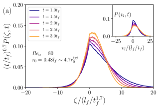
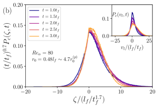
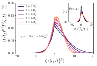
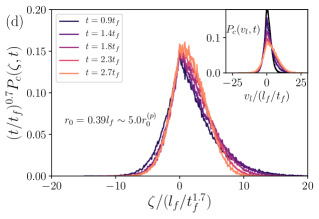
Figure 8: (a) PDFs of the rescaled longitudinal relative velocity, $\zeta(t)=v_{l}(t)/t^{0.7}$ for unconditioned data at different instances $t/t_{f}=1.0,1.5,2.0,2.5,3.0$ for $Re_{\alpha}=80$ with hyperviscosity. Here, the initial separation corresponds to $r_{0}=0.48l_{f}$ which is different from the proper initial separation. It should be noted that $\zeta$ is non-dimensionalized as it is divided by $l_{f}/t_{f}^{1.7}$. Inset: PDFs without re-scaling of the longitudinal relative velocity for the unconditioned data with the initial separation $r_{0}=0.48l_{f}$. (b) Same as (a) albeit for the conditionally sampled data. (c) Same as (a) albeit for $Re_{\alpha}=39$ with normal viscosity at different instances $t/t_{f}=0.9,1.4,1.8,2.3,2.7$. Here, the initial separation corresponds to $r_{0}=0.39l_{f}$. (d) Same as (c) albeit for conditionally sampled data.

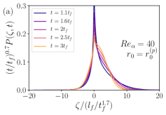
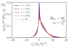
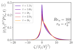
Figure 9: Evolution of PDFs of the rescaled longitudinal relative velocity, $\zeta(t)=v_{l}(t)/t^{0.7}$, of the unconditioned pairs starting from the proper initial separation, $r_{0}^{(p)}$. The PDFs are for (a) $Re_{\alpha}=40$. (b) $Re_{\alpha}=80$. (c) $Re_{\alpha}=160$.

Furthermore, by normalizing with temporal scaling in Eq. (7), the time evolution of the PDF of the conditionally sampled $v_{l}$ becomes self-similar as shown in Fig. 8(b). Here, $P_{c}(A,t)$ corresponds to the conditional PDF for a quantity, $A$. The collapse among different instances does not appear perfect. The collapse around the peak is important because the probability in the tails decays faster than the exponential decay (we compare the degree of the collapse around the peak of the scaled PDF to that of the PDF in the inset). Conversely, the unconditional $v_{l}$ scaled with the same scaling in Eq. (7) does not exhibit the self-similar evolution as shown in Fig. 8(a). Even if we scale the relative velocity with $t^{a/2}$, where the exponent $a$ is measured from $\langle v_{l}(t)^{2}\rangle\propto t^{a}$ shown in Fig. 2(b) for each $r_{0}$, the head parts of the PDFs do not collapse each other as shown in the inset of Fig. 8(a). This implies that the evolution becomes self-similar only for conditionally sampled relative velocity with scaling relations (7). We obtained similar results for the normal viscous case as shown in Fig. 8(c) and (d). It should be noted that in the instances plotted in Fig. 8, the conditional separation, $\langle r^{2}(t)\rangle_{c}$, is forced to agree with the Richardson–Obukhov law. The self-similar evolution of the PDF of $v_{l}(t)$ also holds for unconditioned data starting from the proper initial separation as shown in Fig. 9 for three cases of $Re_{\alpha}$ with hyperviscosity.

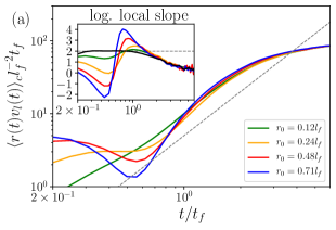
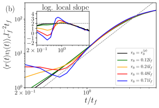
Figure 10: (a) Mean separation rate, $\langle r(t)v_{l}(t)\rangle_{c}$ for conditioned data at various initial separations and for unconditioned data at the proper initial separation, $r_{0}^{(p)}$ for $Re_{\alpha}=40$ with hyperviscosity. Dashed line denotes $t^{2}$ scaling. Inset: The logarithmic local slopes of the data shown in the outset. Dashed line denotes $t^{2}$ scaling. (b) Same as (a) but for $Re_{\alpha}=80$ with hyperviscosity.

Now, we obtain two evidently incompatible results via conditional sampling and selecting the proper initial separation. The second-order moment of the separation, $r(t)$, obeys the K41 scaling (although this is enforced). Conversely, the statistics of relative velocity, $v_{l}(t)$, deviate from the K41 scaling although its evolution is self-similar. As a soft argument in favor of the compatibility between the two results, we examine the mean of the product $r(t)v_{l}(t)$. It should be noted that it is directly related to the evolution of the mean squared separation as $d\langle r^{2}(t)\rangle/dt=2\langle r(t)v_{l}(t)\rangle$, and thus it is termed as the separation rate. As shown in Fig. 10(a), the conditional mean separation rate obeys $\langle r(t)v_{l}(t)\rangle_{c}\propto t^{2}$ as expected given that we enforced the Richardson–Obukhov law. The same $t^{2}$ scaling also holds for the unconditioned mean separation rate starting from the proper initial separation (figure not shown). Evidently, $r(t)$ and $v_{l}(t)$ are statistically dependent, and this is also evident from the kinematics. Hence $\langle r(t)v_{l}(t)\rangle_{c}\neq\langle r(t)\rangle_{c}\langle v_{l}(t)\rangle_{c}$. This indicates that $\langle v_{l}(t)\rangle_{c}\sim t^{0.7}$ does not affect the $t^{2}$ law of the mean separation rate. We observe that the mean separation rate differs from scaling $\langle r(t)\rangle_{c}\langle v_{l}(t)\rangle_{c}\sim t^{3/2+0.7}=t^{2.2}$ , as shown in the insets of Fig. 10(a) and (b), if we consider proper initial separation data as the truly asymptotic data. Therefore, non-Kolmogorov scaling $\langle v_{l}(t)\rangle_{c}\sim t^{0.7}$ is not ruled out due to the dependence despite the Richardson–Obukhov law $\langle r^{2}(t)\rangle_{c}\sim t^{3}$ or, equivalently, the scaling of its time derivative $\langle r(t)v_{l}(t)\rangle_{c}\sim t^{2}$.

IV.2 Quasi-steady state simulation

The non-K41 scaling of the relative velocity as shown in Fig. 6 is not convincing due to the limited scaling range. Here, we increase the scaling range by using the quasi-steady state of the inverse energy-cascade turbulence Kraichnan (1967).

Specifically, we solve the Navier–Stokes equation, Eq. (3), without the hypodrag term, i.e., $\alpha=0$ by maintaining the other parameters as identical to those in Table 1 with hyperviscosity ($h=8$). With respect to averaging, we generate ten random initial data with flat energy spectra extending up to the truncation wavenumber $k_{\max}=(N+2)/3$ with kinetic energy corresponding to $0.010$. Over the ten runs, we take the ensemble average. We perform the simulation with the three resolutions corresponding to $N=1024,2048$, and $4096$. We use the statistically quasi-steady velocity field obtained in time $24.0\leq t\leq 26.5$ for advecting the particle pairs. In the time window, the energy spectrum shows the $k^{-5/3}$ scaling extending down to approximately $k=1$ and the energy grows linearly in time as $\varepsilon t$. Here, we do not use conditional sampling and consider only the particle pairs starting from the proper initial separation estimated as $r_{0}^{(p)}=0.60\times(2\pi/N)$ for each resolution, which amounts to $0.145l_{f}$. The value exceeds those of the statistically steady state, $r_{0}^{(p)}=0.078l_{f}$ at $Re_{\alpha}=39$ with normal viscosity and, $r_{0}^{(p)}=0.089l_{f}$ at $Re_{\alpha}=40$, $r_{0}^{(p)}=0.104l_{f}$ at $Re_{\alpha}=80$, and $r_{0}^{(p)}=0.122l_{f}$ at $Re_{\alpha}=160$ with hyperviscosity. This indicates that $r_{0}^{(p)}$ is affected by the cut-off scale of the inertial range because small-scale quantities are expected to be identical to steady-state simulations.

Figure 11(a) shows $\langle r^{2}(t)\rangle$ satisfying the $t^{3}$ scaling law for longer duration than statistically steady-state cases. In Fig. 11(b), we present $\langle v_{l}^{2}(t)\rangle$ that confirms the non-K41 power-law scaling observed in the statistically steady-state simulations. In more precise terms, from the logarithmic local slope in the inset of Fig. 11(b), we estimate that the scaling exponent is approximately $1.2$. This is consistent with the relation (8). We note that the slopes in the inset of Fig. 11(b) do not exhibit well-developed plateaus.

To summarize Sec. IV, we find the non-K41 scaling law of the relative velocity, $v_{l}(t)\propto t^{0.7}$, and self-similar evolution of the PDFs of $v_{l}(t)$ in the two selected ensembles of the particle pairs. An ensemble corresponds to pairs starting from the proper initial separation $r_{0}^{(p)}$. The other ensemble corresponds to the conditional sampling of the pairs starting from $r_{0}>r_{0}^{(p)}$. For both ensembles, the Richardson–Obukhov law, $\langle r^{2}(t)\rangle=g\varepsilon t^{3}$, is designed to hold.

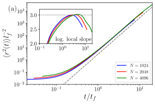
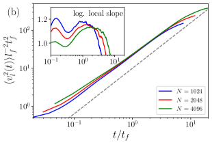
Figure 11: (a) Second-order moments of the relative separations, $\langle r^{2}(t)\rangle$, starting from the proper initial separations in the quasi-steady simulations with resolution $N=1024,2048$, and $4096$. Dashed lines denote $t^{3}$ scaling. Inset: the logarithmic local slope of $\langle r^{2}(t)\rangle$. (b) Same as (a) albeit for the second-order moments of the longitudinal relative velocity, $\langle v_{l}^{2}(t)\rangle$. Dashed line denotes $t^{1.2}$ scaling. Inset: the logarithmic local slope of $\langle v_{l}^{2}(t)\rangle$.

V Concluding Remarks

In the 2D inverse energy-cascade turbulence, we developed conditional sampling to recover the Richardson–Obukhov law by using the relation between the exit-time PDF and Richardson PDF. The conditional squared separation obeys the Richardson–Obukhov law, $\langle r^{2}(t)\rangle_{c}=g\varepsilon t^{3}$, irrespective of the initial separation $r_{0}$. It is noted that we mainly considered $r_{0}>r_{0}^{(p)}$. The fraction of the particle pairs remaining in the conditional sampling increased with increases in $Re_{\alpha}$. This supports our assumption that a bulk of the particle pairs for various initial separations at the moderate Reynolds numbers are in agreement with the Richardson–Obukhov law. As $Re_{\alpha}\to\infty$, deviation in $\langle r^{2}(t)\rangle$ from the Richardson–Obukhov law $g\varepsilon t^{3}$ is likely to vanish. This leads to a conclusion similar to that in a study of the Richardson–Obukhov law in 3D Buaria et al. (2015). Furthermore, conditional sampling indicated that the relative velocity exhibits a different temporal scaling from the prediction of the K41. The results are also obtained for the normal viscous and hyperviscous cases. Therefore, we conclude that the hyperviscosity does not affect the statistical properties of particle pairs.

Evidently, it is always possible to devise conditional sampling to obtain any desired result. To avoid the pitfall, we showed that the conditional statistics are weakly dependent on the parameters, number of the monitored zones $N_{Q}$, and the thresholds of the exit time $\tau$’s. An important finding is that $N_{Q}=1$ is sufficient. This implies that the deviation from the Richardson–Obukhov law is caused in the dissipation range and also by the forcing. It implies that a major deviation is not produced later in the inertial range. The latter implication can result from the intermittency-free Eulerian velocity field of the 2D inverse energy-cascade turbulence.

However, the implications can overlook the behavior of pairs starting from the proper initial separation for which the deviation is negligible. The results indicated that the self-similar evolution of the longitudinal relative velocity is a common feature between the conditionally sampled pairs and unconditional pairs staring from $r_{0}^{(p)}$. This self-similarity is not observed in the unconditional pairs starting from $r_{0}>r_{0}^{(p)}$. It should be noted that the self-similarity emerges only with the non-K41 power law of the equal-time relative velocity correlation, namely the relation (8). Furthermore, the self-similarity among the PDFs of various instances indicates that the non-K41 scaling differs from the intermittency observed in the Eulerian velocity increments of 3D turbulence. We argued that the non-K41 velocity scaling is not immediately ruled out by the enforced Richardson–Obukhov law.

The non-K41 power-law scaling obtained here, $\langle v_{l}^{2}(t)\rangle\propto t^{1.23}$, exhibits an exponent that differs from the K41 prediction, $\langle v_{l}^{2}(t)\rangle\propto\varepsilon t$. This can be qualitatively explained by the following behavior of the two-time correlation function of the Lagrangian relative velocity, $\langle\delta{\bm{v}}(s_{1})\cdot\delta{\bm{v}}(s_{2})\rangle$, where $\delta{\bm{v}}(t)={\bm{v}}(t|{\bm{a}}+{\bm{r}}_{0})-{\bm{v}}(t|{\bm{a}})$. We use DNS data starting from the proper initial separation and plot the correlation function in the 2D space $(s_{1},s_{2})$. This type of a plot is presented for the 3D case in Ishihara and Kaneda (2002). The two-time correlation is characterized by two functional forms as follows: one along the diagonal line and the other along the line perpendicular to the diagonal line. The preliminary study suggests that the two functional forms exhibit distinct self-similar functions. Specifically, we speculate that the self-similarity of the latter one along the line normal to the diagonal line leads to the deviation from the K41 scaling of the relative velocity. Thus, the non-K41 behavior of the velocity can be ascribed to the temporal correlation, which is ignored in the K41 argument Falkovich et al. (2001); Ogasawara and Toh (2006b). A future study will detail the two-time correlation.

The results obtained with the enforced Richardson–Obukhov law lead us to conclude that self-similarity of the relative velocity with the non-K41 scaling plays an indispensable role in the Richardson-Obukhov law of the squared separation. The condition is fulfilled for the pairs starting from the proper initial separation, $r_{0}^{(p)}$. An explanation for this is absent. It can be cautiously stated that quantitative aspects of the proper initial separation depend on the forcing because $r_{0}^{(p)}<l_{f}$.

We qualitatively discuss the characteristics of the special particle pairs initially separated by $r_{0}^{(p)}$ with respect to conditional sampling. The conditional sampling classifies particle pairs into three groups as follows: (i) removed particles for $r_{0}>r_{0}^{(p)}$, (ii) removed particles for $r_{0}<r_{0}^{(p)}$, and (iii) unremoved particles. It should be noted that we here include the result of the conditional sampling for $r_{0}<r_{0}^{(p)}$. We argue that the nature of each group can be different. For $r_{0}>r_{0}^{(p)}$, the power-law exponent of the unconditional $\langle r^{2}(t)\rangle$ is lower than the Richardson–Obukhov exponent $3$ as shown in Fig. 2(a). In the conditional sampling, we remove particle pairs in which the exit time per the mean is lower than the threshold, $\tau$. Subsequently, the power-law exponent of $\langle r^{2}(t)\rangle_{c}$ rises to 3. This implies that the removed pairs for $r_{0}>r_{0}^{(p)}$ lower the power-law exponent of $\langle r^{2}(t)\rangle$.

A physical interpretation can be as follows. The removed pairs in the group (i) typically either hardly expand and consequently stay at around the initial separation or exit from the inertial range and then behave as standard Brownian particles while the unremoved particle pairs are still in the inertial range. Conversely, for $r_{0}<r_{0}^{(p)}$, the power-law exponent of $\langle r^{2}(t)\rangle$ is larger than $3$ as shown in Fig. 2(a). In the conditional sampling, we remove the particle pairs in which the exit time per the mean is within the interval, $[\tau_{1},\tau_{2}]$. Subsequently the power-law exponent of $\langle r^{2}(t)\rangle_{c}$ decreases to 3. This implies that the removed pairs for $r_{0}<r_{0}^{(p)}$ increase the power-law exponent of $\langle r^{2}(t)\rangle$. A physical interpretation is as follows. The removed pairs for $r<r_{0}^{(p)}$ in the group (ii) typically expand anomalously fast through the inertial range while the unremoved particle pairs are still in the inertial range. The pairs in the group (iii), namely, the unremoved pairs in the conditional sampling regardless of the initial separation, are typically those that satisfy the Richardson–Obukhov law. The results indicated that the fraction of the pairs belonging to the groups (i) and (ii) significantly depend on the initial separation. Groups (i) and (ii) are potentially related to the extreme events Scatamacchia et al. (2012); Biferale et al. (2014). We now return to the proper initial separation. It is inferred that the effects of the two removed groups on $\langle r^{2}(t)\rangle$ are balanced at the proper initial separation. Hence, the Richardson–Obukhov law recovers for $r_{0}^{(p)}$ without the conditional sampling because contamination from the two groups is cancelled. Additionally, the cancelling also supports the dependence of the proper initial separation on the width of the inertial range mentioned in Sec.IVB, i.e., $r_{0}^{(p)}$ increases with $Re_{\alpha}$. The number of particle pairs in the group (i) that exit the inertial range relatively fast and separate based on the $t^{2}$ law decreases inversely with the width of the inertial range, and the value of $r_{0}^{(p)}$ should be increased to cancel the anti-effects of groups (i) and (ii) on the scaling exponent.

We observed the non-Kolmogorov scaling law of the Lagrangian velocity. Evidently, an important question is whether or not the deviation from the K41 exponent persists when the Reynolds number increases. The trend shown in Fig.7(a) indicates that the deviation persists. However, it is not possible to eliminate the possibility that the Kolmogorov scaling law $\langle v_{l}^{2}(t)\rangle\propto t$ prevails at significantly higher Reynolds numbers. To address the question, an approach that differs from numerical simulation such as Lagrangian two-point closure theory, is preferable.

Our conditional sampling method can be easily adopted to 3D turbulence. However, the insights gained in 3D should significantly differ from those obtained here in the 2D inverse energy-cascade turbulence. Physics of the 2D energy inverse-cascade turbulence considerably differs from that of the 3D turbulence although the scaling argument using the dissipation rate (i.e., the mean energy flux) leads to the same prediction of scaling exponents of various statistics. The main difference is that it is necessary to add the forcing at a small scale for the 2D case. This implies that Lagrangian particles in 2D turbulence are more directly affected by the forcing than those in 3D turbulence. A future study will present a detailed analysis of the 3D problem.