[table]capposition=top

Explicit Estimation of Derivatives from Data and Differential Equations by Gaussian Process Regression

Abstract

In this work, we employ the Bayesian inference framework to robustly estimate the derivatives of a function from noisy observations of only the function values at given location points, under the assumption of a physical model in the form of differential equation governing the function and its derivatives. To overcome the instability of numerical differentiation of the fitted function solely from the data or the prohibitive costs of solving the differential equation on the whole domain, we use the Gaussian processes to jointly model the solution, the derivatives, and the differential equation, by utilising the fact that differentiation is a linear operator. By regarding the linear differential equation as a linear constraint, we develop the Gaussian process regression with constraint method (GPRC) at Bayesian perspective to improve the prediction accuracy of derivatives. For nonlinear equations, we propose a Picard-iteration approximation of linearization around the Gaussian process obtained only from data to iteratively apply our GPRC. Besides, a product of experts method is applied if the initial or boundary condition is also available. We present several numerical results to illustrate the advantages of our new method and show the new estimation of the derivatives from GPRC improves the parameter identification with less data samples.

Keywords: estimation of derivative, Gaussian process, Bayesian inference

1 Introduction

To infer a nonlinear function from its noisy measurements at a given set of inputs is a classical statistical learning problem and a vast of well-established methods, ranging from polynomial and spline to kernel method and neural network, are available for many important applications[9]. However, if the interest is the derivatives and there is no additional observations of derivatives, the problem of estimating derivatives is more challenging and subtle than estimating the function itself and less attentions have been given to this issue. When the measurements are on the gridded data, the naive method of finite difference deteriorates the accuracy of numerical derivatives and the algorithm may become extremely unstable if the data is scarce and the order of derivatives is high. The modern machine learning approach [21, 9] enforces certain regularity in learning the function and practically relies on cross-validation technique to select the right model. But the lack of data from derivatives generally hinders the direct use of this framework. In applications, many practitioners simply take the symbolic or numerical differentiation after the function is trained first, and seem to pay less attention to the accuracy and robustness of the obtained derivatives.

As we will explain soon, many applications in need of robust estimation of derivatives arise from various problems related to differential equation (DE) models which the function and its derivatives should satisfy. This situation in fact offers an extra advantage for estimating the function and derivatives. In this paper, we shall assume that the observation data are the measurements (subject to uncertainty noise) of the solution of the DE model and the (partial or complete) information of the underlying DE model is also known to us. We study the problem of efficiently and robustly estimating the function and its derivatives up to the order of interest within a Bayesian inference framework, by taking into account of the solution observations and the corresponding DE model simultaneously and intrinsically. In the next, before we present our main ideas, we provides some further backgrounds on the importance of estimate of derivatives.

Differential equations which include ordinary differential equation (ODE) and partial differential equation (PDE) are used to model a wide variety of physical phenomena such as heat transfer, electromagnetism, and structural deformations. In physics or chemistry problems, the state, which is the solution of the model, and its derivatives (time derivative or spatial gradient) usually have specific meanings, e.g., location and velocity in Newton mechanics, electric potential and electric field in electrostatics. In ODE models, often the time derivative of a state variable is of as much interest as the state variable itself [20]. Many physical constitutive laws appear in form of PDEs linking the derivatives to the state variable. In the deterministic PDE, the derivatives are generally computed by numerical differentiation techniques after the solution is computed from numerical methods like finite element method, for instance. In general, the convergence order of errors for such derivatives is one order lower than the convergence rate for the solution itself. In history, this accuracy degradation problem for the gradient is alleviated to certain extent by the mixed finite element method ([2]), which treats the gradient as an independent variable and constructed an extended system jointly for the solution and its gradient. When the PDE models have random or missing parameters/coefficients, the estimate of the solution and the derivatives of the solution becomes a non-trivial task because the numerical solution is typically a random function with uncertainties inherited from the randomness of the PDE or the noisy measurement. Various numerical experiments suggest that a direct numerical difference scheme for the derivative for a random function usually lacks of robustness and the higher order the derivatives, the less accuracy of the estimation.

The demand of robust estimation of derivatives becomes more critical when a DE model is supplemented with available data as the measurement of the state variable, while the DE model is too complicated to solve precisely or is incomplete with missing parameters or with random coefficients. One of such scenarios is the problem of identifying the missing information of a DE model from the noisy measurement of the state variable [22, 16, 10, 23, 3, 17, 13, 15]. In these problems, the noisy measurements of the solution are given at randomly drawn or deliberately chosen points and optimization frameworks are proposed to identify the missing information in the DE. In these optimization problems, the state variables and its all derivatives appearing in the DEs are required as the input information, however there is no measurement data for the derivatives. One mainstream approach is the two-stage procedure [22, 10, 12], which in the first stage estimates the function and its derivatives from noisy observations using data smoothing methods without considering differential equation models, and then in the second stage identifies the missing parameters by the method of least squares. Many data smoothing methods are applicable in the first stage to fit the state function, such as polynomial interpolation [17], local polynomial regression [10] and spline-based approach [22]. These methods are easy to implement and can achieve excellent fitting result for the state function itself, however the derivatives of the fitted function in fact are not as accurate and robust as the function itself, which may significantly affect the parameter identification in the second stage. So, the main drawback of the two-stage method is that the underlying differential equation is not fully utilized.

There have been efforts to incorporate the DE model in the first stage to improve the accuracy of both the state function and its derivatives appearing in the DE model. In [23] X. Xun et al proposed to incorporate the differential equation as a penalty term in the first stage, where the solution is expressed by B-spline basis functions and the derivatives are based on analytical derivatives of B-splines. This produces more reliable derivatives for the second stage and finally improves the accuracy of estimating parameters significantly, particularly for the parameters associated with derivatives. However, this approach of treating differential equation as a squared penalty gives rise to difficult optimization problem or Markov chain Monte Carlo step [23].

In view of the critical importance of robust estimation of derivatives for the above applications, we focus on how to combine the data of the state function and the DE information to improve the derivative estimation by a new approach. We propose a new statistical approach based on Gaussian process regression (GPR) to efficiently and robustly predict the derivatives in need. Compared with the basis-function expansion method and MCMC Bayesian approach, the Gaussian process (GP) model [19] is flexible and efficient for fitting noisy data. The prior knowledge can also be easily encoded by the covariance of the GP. More importantly, the derivatives of a GP is also a GP since taking derivatives is a linear operation. When the DE model is also linear, we can gain favourable advantages from this linearity property of GP.

To achieve our goal, we build our method, with the name Gaussian Process Regression with Constraint (GPRC), on the following ideas. Firstly, we treat the state variable and the derivatives appearing in the differential equation jointly as a multi-dimensional GP to leverage the advantage of a jointly Gaussian distribution over the function and its derivatives [19]. Secondly, to take account of the differential equation that state and derivatives should satisfy, we exploit the fact that the residual of the differential operator corresponding to the DE should be zero, which provides the zero-valued measurements of the residual. We model the residual for linear DEs as a mean-zero prior Gaussian with a small variance. Then, the observations for training the GP are the paired values of the state variable and the residual. In other words, the available information of DE is treated as additional constraint for the multi-dimensional GP of state and derivatives should satisfy. Thirdly, to generalize our method to nonlinear equations, we consider a Picard approximation of linearization in which the nonlinear part is approximated by linearization around a function obtained from the standard GPR first without using the equation, and the multi-dimensional GP is then recursively updated based on the linearized equation. Lastly, in the prediction for the function and its derivatives on a new test location, the zero-valued residual observation from the DE model on the test location is also exploited to further strengthen the prediction accuracy of the derivatives. In addition, if the linear boundary/initial condition (BC/IC) is available, they can also be added as one of linear constraints that the GP should satisfy like the DE itself, by the product of experts method [11, 4, 1]. Our method can be applied to the parameter identification problems but it certainly fits in any application which needs a robust scheme of derivative estimation when a differential equation model underlying the data is available.

In our numerical experiments, we shall demonstrate the effectiveness of this new method GPRC by comparing the obtained derivatives with the results from the traditional GPR on a few linear DE models. We also present a nonlinear Van der Pol equation with a parameter $\mu$. Based on the dataset corresponding to the ground-truth $\mu^{*}=0.5$, we not only show a better estimation of the derivatives for this $\mu^{*}$, but also illustrate the supremacy of our method when applied to identify $\mu^{*}$ when the observations are scarce. In this example, the traditional GPR fails to find the correct $\mu^{*}$ because of the inaccurate estimation of derivatives.

In the last part of this section, we selectively comment on some general works related to the GP. For the use of GP to solve differential equations, there has been a considerable amount of literature. For example, [8] has used GP to solve linear differential equations with noisy forcing terms. The use of GPR for inference related to differential equation is intensively studied in the communities of machine learning [18, 1] and statistics [10, 23]. For the idea of exploring the GP for the state function and the state-derivatives jointly rather separately, [4] focused on a Bayesian inference of the parameters in ODE models. [7] used the GP prior in Bayesian method to infer parameters in the ODE models of chemical networks. For recent advancement of parameter identification, [3, 17] worked on the PDE “discovery” problem by $\ell_{0}$ or $\ell_{1}$ optimization to learn a spars set of coefficients in PDE. [15, 13] worked with the scarce and noisy measurement of both the state variable and a black-box forcing term in the PDE and the joint GPR model is applied to solve the solution function and infer the forcing-term function. But in existing literature, we have not yet seen a specific method for efficiently and robustly processing the derivative estimation if the differential equation is also given.

The structure of the paper is organized as follows: We first formulate the problem setup in Section 2. Our GPRC method for estimating the state and its derivatives is presented in Section 3. A product of experts method for initial or boundary conditions is introduced in Section 4. Numerical examples are presented in Section 5 to demonstrate the effectiveness of the proposed method and the extension to nonlinear differential equation problems (Section 5.3). Lastly, in Section 5.4, we use the nonlinear toy model to illustrate the new estimation of derivatives by GPRC improves the quality the parameter identification with less data samples. Section 6 offers some closing remarks and outlooks.

2 Problem setup

In general we formulate the differential equation system as a multidimensional dynamic process and view the ordinary differential equation as a one-dimensional partial differential equation case. The solution function is denoted as $u({\bm{x}})$, where ${\bm{x}}=(x_{1},\dots,x_{D})^{T}\in\mathbb{R}^{D}$. The PDE is modeled as

$$\mathcal{F}({\bm{x}},u,\frac{\partial u}{\partial x_{1}},\dots,\frac{\partial u}{\partial x_{i}},\dots,\frac{\partial^{2}u}{\partial x_{i}\partial x_{j}},\dots)=0,$$ (2.1)

where the left-hand side of Eq. (2.1) consists of the state $u({\bm{x}})$ and its partial derivative terms ($\frac{\partial u}{\partial x_{i}},\frac{\partial^{2}u}{\partial x_{i}\partial x_{j}},\dots,$). In practice, we only can directly observe the noisy observation $y({\bm{x}})$ instead the state $u({\bm{x}})$ . We assume that $u({\bm{x}})$ is observed with measurement error and specifically, the noisy measurements satisfy

$$y_{i}=u({\bm{x}}_{i})+\epsilon_{i},$$ (2.2)

where $i=1,\dots,n$, is the observation index, each point ${\bm{x}}_{i}\in{\mathbb{R}}^{D}$ and $\epsilon_{i}$ is the measurement error, also called noisy/observation error. Assumption is made that the error $\epsilon_{i}$ is an iid random variable and follows a Gaussian distribution with mean $0$ and variance $\sigma_{u}^{2}$.

Our objective is to estimate the state $\bm{u}$ and its derivative terms $\frac{\partial^{K}\bm{u}}{\partial^{k}x_{i}\partial^{K-k}x_{j}}$, $k=0,\dots,K$, $K=1,2,\dots$, from the noisy data $({\bm{x}}_{i},y({\bm{x}}_{i}))$ together with the equation (2.1), and to quantify the uncertainty of our estimations. The estimation problem in linear dynamic process where $\mathcal{F}$ in (2.1) is a linear operator is more fundamental and has been serving as the very start of nonlinear equations[15, 18, 8]. To discuss the linear equation case first, we use $\mathcal{L}u({\bm{x}})$ to denote $\mathcal{F}({\bm{x}},u,\frac{\partial{\bm{u}}}{\partial x_{i}},\dots,\frac{\partial^{2}{\bm{u}}}{\partial x_{i}\partial x_{j}},\dots)$ as a function of ${\bm{x}}$ if $\mathcal{F}$ is a linear operator.

3 Methodology

The proposed algorithm for estimating the state and its derivatives, employs Gaussian process prior that is tailored to the corresponding differential operators.

3.1 Gaussian process regression

Specifically, the method starts by assuming that $u({\bm{x}})$ is a Gaussian process with the zero mean and the covariance function $k_{uu}({\bm{x}},{\bm{x}}^{\prime};\bm{\gamma})$, which is denoted as

$$u({\bm{x}})\sim\mathcal{GP}(0,k_{uu}({\bm{x}},{\bm{x}}^{\prime};\bm{\gamma})),$$ (3.1)

where $\bm{\gamma}$ denotes the hyper-parameters of the kernel function $k_{uu}$. This means that $\mathbb{E}[u({\bm{x}})]\equiv 0$ and $\mathrm{Cov}(u({\bm{x}}),u({\bm{x}}^{\prime}))=k_{uu}({\bm{x}},{\bm{x}}^{\prime};\bm{\gamma})$. The kernel $k_{uu}$ allows us to encode any prior knowledge we may have about $u({\bm{x}})$, and can accommodate the approximation of arbitrarily complex functions. The choice of the specific form of $k_{uu}$ will be discussed later.

The key property of Gaussian process in our favor is that any linear transformation, such as differentiation and integration, of a Gaussian process is still a Gaussian process. With the assumption (3.1), we consider the linear differential operator, $\mathcal{L}$, acted on $u({\bm{x}})$. Then the function $\mathcal{L}u({\bm{x}})$ is also a mean-zero Gaussian process

$$\mathcal{L}u({\bm{x}})\sim\mathcal{GP}(0,k_{LL}({\bm{x}},{\bm{x}}^{\prime}))$$ (3.2)

where $k_{LL}({\bm{x}},{\bm{x}}^{\prime})=\mathrm{Cov}(\mathcal{L}u({\bm{x}}),\mathcal{L}u({\bm{x}}^{\prime}))$ denotes the covariance function of $\mathcal{L}u$ between ${\bm{x}}$ and ${\bm{x}}^{\prime}$. The following fundamental relationship between the kernels $k_{uu}$ and $k_{LL}$ is well-known (see e.g. [19, 8]),

$$k_{LL}({\bm{x}},{\bm{x}}^{\prime};\bm{\gamma})=\mathcal{L}_{\bm{x}}\mathcal{L}_{{\bm{x}}^{\prime}}k_{uu}({\bm{x}},{\bm{x}}^{\prime};\bm{\gamma}).$$ (3.3)

Here we add the subindex in the linear differential operator $\mathcal{L}$ to specify the differentiation is for ${\bm{x}}$ or ${{\bm{x}}}^{\prime}$ variable in the kernel function. $k_{uu}$ and $k_{LL}$ share the same hyper-parameter $\bm{\gamma}$. Simiarly, for the covariance between $u$ and $\mathcal{L}u$, $k_{uL}({\bm{x}},{\bm{x}}^{\prime})=\mathrm{Cov}(u({\bm{x}}),\mathcal{L}u({\bm{x}}^{\prime}))$ and $k_{Lu}({\bm{x}},{\bm{x}}^{\prime})=\mathrm{Cov}(\mathcal{L}u({\bm{x}}),u({\bm{x}}^{\prime}))$, we have

$$k_{uL}({\bm{x}},{\bm{x}}^{\prime};\bm{\gamma})=\mathcal{L}_{{\bm{x}}^{\prime}}k_{uu}({\bm{x}},{\bm{x}}^{\prime};\bm{\gamma}),~{}\text{ and }~{}k_{Lu}({\bm{x}},{\bm{x}}^{\prime};\bm{\gamma})=\mathcal{L}_{{\bm{x}}}k_{uu}({\bm{x}},{\bm{x}}^{\prime};\bm{\gamma}).$$ (3.4)

Since we shall work on the differential equation $\mathcal{L}u({\bm{x}})=0$, we introduce a random function $r({\bm{x}})$ as the residual of the linear differential equation $\mathcal{L}u=0$ for convenience:

$$r({\bm{x}}):=\mathcal{L}u({\bm{x}}).$$ (3.5)

We refer the original equation as the equation constraint, $r({\bm{x}})=0$, and the equation will be interpreted later as the observation of zero values of the function $r({\bm{x}})$ at any point ${\bm{x}}$, in a similar way to the observation $y_{i}$ of $u({\bm{x}})$ at ${\bm{x}}_{i}$. With the given prior of the GP $u({\bm{x}})$, we then have the the prior for the pair $(u({\bm{x}}),r({\bm{x}}))$. The covariances above for $u$ and $\mathcal{L}u$ can be rewritten as

$$\begin{split}k_{rr}({\bm{x}},{\bm{x}}^{\prime};\bm{\gamma})&=\mathcal{L}_{\bm{x}}\mathcal{L}_{{\bm{x}}^{\prime}}k_{uu}({\bm{x}},{\bm{x}}^{\prime};\bm{\gamma}),\\ k_{ur}({\bm{x}},{\bm{x}}^{\prime};\bm{\gamma})&=\mathcal{L}_{{\bm{x}}^{\prime}}k_{uu}({\bm{x}},{\bm{x}}^{\prime};\bm{\gamma}),\\ k_{ru}({\bm{x}},{\bm{x}}^{\prime};\bm{\gamma})&=\mathcal{L}_{{\bm{x}}}k_{uu}({\bm{x}},{\bm{x}}^{\prime};\bm{\gamma}),\end{split}$$ (3.6)

respectively.

So the equation residual $r({\bm{x}})$ is also a Gaussian process, whose kernel is related to the derivatives of the kernel of $u({\bm{x}})$. Based on the Gaussian assumption and the covariance expression between $u$ and $r$ in (3.6), a joint inference framework of Gaussian process regression for the available observation data of $u$ and $r$ can be naturally constructed. By interpreting the equation $r=\mathcal{L}u=0$ as the constraint of the function $r$, we refer this approach as Gaussian Process Regression with Constraint (GPRC). GPRC will significantly improve the accuracy of estimation of solution and its derivatives due to the additional equation information. The advantages in the comparison with standard Gaussian process regression (without constraint) will be shown in Section 5.

Remark 1.

The linear differential operator can be easily generalized to an affine operator, i.e., the equation $\mathcal{L}u({\bm{x}})=f({\bm{x}})$. Then the linear constraint $r({\bm{x}})=0$ should be modified as $r({\bm{x}})=f({\bm{x}})$. To be concise, we present our ideas and methods only for the linear case $f({\bm{x}})=0$.

The differential equation discussed above is the linear constraint, i.e., $r=\mathcal{L}u$ is a linear mapping of $u$. For the non-linear differential equation $\mathcal{F}(u)=0$, we propose a linearizaiton strategy to make GPRC applicable to nonlinear problems. To illustrate idea, consider a special case $\mathcal{F}(u)=\mathcal{L}(u)+\mathcal{N}(u)$ for example, where $\mathcal{N}$ is the nonlinear part. We apply the standard GPR only from the data $\{{\bm{x}}_{i},y_{i}\}$ to train a GP $u_{0}$, and then apply the GPRC to the affine constraint $\mathcal{F}_{0}(u):=\mathcal{L}(u)+\mathcal{N}(u_{0})=0$ and the data $\{{\bm{x}}_{i},y_{i}\}$ to train $u$ as an update of $u_{0}$. This approach can be implemented recursively and is a type of Picard iteration per se. The stopping criterion is based on the Root Mean Square Error (RMSE) of the true (nonlinear) residual. In Section 5.3, we shall specifically show how to apply this idea to a nonlinear oscillator equation.

3.2 Kernel

The kernel (covariance function) is the crucial ingredient in a Gaussian process predictor, as it encodes our assumptions about the function we wish to learn. Without loss of generality, the Gaussian prior of the solution used in this work is assumed to have a squared exponential covariance function (other kinds of kernels are also suitable in this framework), i.e.,

$$k_{uu}({\bm{x}},{\bm{x}}^{\prime},\bm{\gamma})=\gamma^{2}_{\alpha}\exp(-\frac{1}{2}||{\bm{x}}-{\bm{x}}^{\prime}||^{2}_{\bm{\gamma}_{l}})$$ (3.7)

where $\gamma^{2}_{\alpha}$ is a variance parameter, ${\bm{x}}$ is a $D$-dimensional vector that includes spatial and/or temporal coordinates, the norm $||\cdot||_{\bm{\gamma}_{l}}$ is defined as

$$||\bm{v}||_{\bm{\gamma}_{l}}=(\bm{v}^{T}\bm{\gamma}_{l}\bm{v})^{\frac{1}{2}},~{}\bm{\gamma}_{l}=\mbox{diag}(\gamma_{l1},\dots,\gamma_{lD}).$$ (3.8)

$\bm{\gamma}_{l}$ is the length scale parameter and $\bm{\gamma}=(\gamma_{\alpha},\bm{\gamma}_{l})$. The squared exponential covariance function chosen above implies smooth approximations. More complex function class can be accommodated by appropriately choosing kernels. For example, non-stationary kernels employing nonlinear warpings of the input space can be constructed to capture discontinuous response. In general, the choice of kernels is crucial and in many cases still remains an art that relies on one’s ability to encode any prior information (such as known symmetries, invariant, etc.) into the regression scheme. In our problem here related to the differential operator $\mathcal{L}$, we require that the kernel satisfies the regularity such that the derivatives of the kernel, $\mathcal{L}_{\bm{x}}\mathcal{L}_{{\bm{x}}^{\prime}}k_{uu}({\bm{x}},{\bm{x}}^{\prime})$, which is the covariance function of $\mathcal{L}u$, are at least continuous. Our choice of squared exponential covariance function surely satisfies this requirement.

The kernel $k_{Lu}({\bm{x}},{\bm{x}}^{\prime};\bm{\gamma})$ can be easily computed based on (3.7). For instance the kernel of first order derivative term $\partial_{\bm{x}}u({\bm{x}})$ can be expressed as:

$$k_{Lu}({\bm{x}},{\bm{x}}^{\prime};\bm{\gamma}):=\frac{\partial k_{u,u}({\bm{x}},{\bm{x}}^{\prime};\bm{\gamma})}{\partial{\bm{x}}}\\ =-k_{uu}({\bm{x}},{\bm{x}}^{\prime},\bm{\gamma})\bm{\gamma}_{l}({\bm{x}}-{\bm{x}}^{\prime})$$ (3.9)

The expressions of other kernel for a general linear differential operator, such as $\frac{\partial^{2}k_{u,u}({\bm{x}},{\bm{x}}^{\prime};\bm{\gamma})}{{\partial{\bm{x}}}^{2}}$, $\frac{\partial^{2}k_{u,u}({\bm{x}},{\bm{x}}^{\prime};\bm{\gamma})}{\partial{\bm{x}}\partial{\bm{x}}^{\prime}}$ can be computed similarly.

Due to the irreducible measure noise in (2.2), the covariance matrix in the prior of $u({\bm{x}})$, $k_{uu}$ usually needs to be added with a noise kernel $\sigma_{u}^{2}\bm{I}_{u}$, $\bm{I}_{u}$ is identity matrix and the parameter of variance $\sigma_{u}^{2}$ can be optimized with the kernel parameters $\bm{\gamma}$ together. In a similar style, we can also introduce a small parameter $\sigma_{r}^{2}\bm{I}_{r}$ for the residual function $r({\bm{x}})$.

3.3 Training

The training process is to find the optimal parameters $\bm{\gamma}$ and $\sigma_{u}^{2}$ by maximum likelihood estimation (MLE). Since all GPs appearing above share the same set of hyper-parameters $\bm{\gamma}$, this helps reduce computational burden.

Given $n$ noisy observations of the state $u$ at $n$ points $\{{\bm{x}}_{i}:1\leq i\leq n\}$, we denote the state vector ${\bm{y}}\equiv[y_{1},y_{2},\dots,y_{n}]^{T}\in{\mathbb{R}}^{n\times 1}$, the residual vector $\bm{r}\equiv[r_{1},r_{2},\dots,r_{n}]^{T}\in{\mathbb{R}}^{n\times 1}$ and the training point matrix $X\equiv[{\bm{x}}_{1},{\bm{x}}_{2},\dots,{\bm{x}}_{n}]^{T}\in{\mathbb{R}}^{n\times D}$. Let $Y=\begin{bmatrix}{\bm{y}}\\ \bm{r}\end{bmatrix}\in{\mathbb{R}}^{2n}$. Then the negative log marginal likelihood of $p(Y|\bm{\gamma},\sigma^{2}_{u})$ has the following expression

$$\begin{split}-\log p(Y|\bm{\gamma},\sigma^{2}_{u})=\frac{1}{2}\log(\det{K})+\frac{1}{2}Y^{T}K^{-1}Y+\frac{n}{2}\log 2\pi,\end{split}$$ (3.10)

where the $2n\times 2n$ matrix $K$ is defined by

$$K=\begin{bmatrix}&K_{uu}+\sigma^{2}_{u}I&K_{ur}\\ &K_{ru}&K_{rr}+\sigma^{2}_{r}I\end{bmatrix},$$

The matrices $K_{uu},K_{ur}$, $K_{ru}$ and $K_{rr}$ correspond to, respectively, the kernel functions $k_{uu},k_{ur},k_{ru}$ and $k_{rr}$ in (3.7) and (3.6), evaluated at the $n$ points $\{{\bm{x}}_{i}\}$.

To compute the optimal kernel hyperparameters $\bm{\gamma}$ and observation noise variance $\sigma^{2}_{u}$, a Quasi-Newton optimizer L-BFGS is employed to minimize the negative log marginal likelihood (3.10). Cholesky factorarization of $K$ is used to compute both the inverse and the determinant.

It is noteworthy that the constraint from the DE model should be rigorous, which means $\sigma^{2}_{r}$ should be exactly zero. However, for numerical stability and statistical generalization, we add a regularization $\sigma^{2}_{r}$ term onto the constraint covariance matrix $K_{rr}$ and then $\sigma^{2}_{r}$ is a hyper-parameter to tune. In principle, the optimal value of $\sigma^{2}_{r}$ is related to the complexity of model (e.g., the choice of the kernel), the variance of the measurement noise (i.e., $\sigma_{u}^{2}$) in the data, and the DE model itself (e.g., the order of derivatives in appearance). The practical optimal $\sigma^{2}_{r}$ can be determined by any standard parameter-tuning method like cross-validation. A note is that $\sigma^{2}_{r}$ should be larger than $\sigma_{u}^{2}$ since taking derivatives in general amplifies the noise (with high frequency). We empirically find a tenfold size of $\sigma_{u}^{2}$ seems satisfactory if the DE model has up to a second order derivative.

3.4 Prediction

After the hyper-parameters in the GPRC are computed, the prediction of the function $u({\bm{x}})$ or its derivatives of interest, denoted as a function $l({\bm{x}})$ (e.g., $l({\bm{x}})=\partial_{{\bm{x}}}u({\bm{x}})$), at a new test point ${\bm{x}}_{*}$ is described below. The covariance function of the GP $l({\bm{x}})$ is denoted by $k_{ll}({\bm{x}},{\bm{x}}^{\prime})$ by the convenction.

With a given point ${\bm{x}}_{*}$, the differential equation provides the fact $r({\bm{x}}_{*})=0$, which is a useful observation to incorporate the Bayesian inference. To enhance this condition locally, we actually consider a small neighbourhood around ${\bm{x}}_{*}$ and choose $m$ equally-spaced points in this neighbourhood. The set $\chi$ is similar to the window/scale concept in local polynomial regression and thus adaptive strategy is possible ([6]). We refer the collection of these $m$ points as the extended set $\chi:=\{{\bm{x}}_{*}^{j}:1\leq j\leq m\}$ and by the differential equation, we have the equation constraints in this extend set, i.e., $\bm{r}_{\chi}=\bm{0}$. These points ${\bm{x}}_{*}^{j}$ are supposed to resolve a characteristic length for the residual process $r({\bm{x}})$. So, the size of the extend set $\chi$ and the number $m$ are related to the correlation length of the residual GP, specifically, $1/\bm{\gamma}_{l}$ with $/\bm{\gamma}_{l}$ and their choice is a balance between computational cost and the prediction accuracy from the DE model. In practice, just a few number of $m$ in each dimension is sufficient and we will give some details in Section 5.

Let $u_{*}$ and $l_{*}$ represent the state and its derivative at the test point ${\bm{x}}_{*}$, respectively. Adding the equation constraint vector $\bm{r}_{\chi}$ at the points in the extend set $\chi$, we have the joint distribution for the Gaussian priors

$$\begin{bmatrix}\begin{bmatrix}{\bm{y}}\\ \bm{r}_{\chi}\end{bmatrix}\\ u_{*}\\ l_{*}\end{bmatrix}=\mathcal{N}\Big{(}\begin{bmatrix}\begin{bmatrix}\bm{0}\\ \bm{0}\end{bmatrix}\\ 0\\ 0\end{bmatrix},\begin{bmatrix}\widehat{K}_{u\bm{r}_{\chi}}&\begin{matrix}K_{uu_{*}}&K_{ul_{*}}\\ K_{\bm{r}_{\chi}u_{*}}&K_{\bm{r}_{\chi}l_{*}}\end{matrix}\\ \begin{matrix}K_{uu_{*}}^{T}&K_{\bm{r}_{\chi}u_{*}}^{T}\\ K_{ul_{*}}^{T}&K_{\bm{r}_{\chi}l_{*}}^{T}\end{matrix}&\begin{matrix}K_{u_{*}}&K_{u_{*}l_{*}}\\ k_{u_{*}l_{*}}^{T}&K_{l_{*}}\end{matrix}\end{bmatrix}\Big{)},$$ (3.11)

where

$$\widehat{K}_{u\bm{r}_{\chi}}=\begin{bmatrix}K_{u}&K_{u\bm{r}_{\chi}}\\ K_{u\bm{r}_{\chi}}^{T}&K_{\bm{r}_{\chi}}\end{bmatrix}\in{\mathbb{R}}^{(n+m)\times(n+m)},$$

$K_{u}=K_{uu}+\sigma^{2}_{u}\bm{I}_{u}\in{\mathbb{R}}^{n\times n}$, $K_{\bm{r}_{\chi}}=K_{\bm{r}_{\chi}\bm{r}_{\chi}}+\sigma^{2}_{r}\bm{I}_{r}\in{\mathbb{R}}^{m\times m}$, $K_{u_{*}}=k_{uu}({\bm{x}}_{*},{\bm{x}}_{*})$, $K_{l_{*}}=k_{ll}({\bm{x}}_{*},{\bm{x}}_{*})$ and other matrices, e.g., $K_{uu_{*}},K_{u\bm{r}_{\chi}},K_{u_{*}l_{*}}$ are defined similarly via the kernels $k_{uu}$, $k_{ur}$ and $k_{ul}$. As mentioned above, $\bm{r}_{\chi}=\mathcal{L}u(\chi)$ is actually known as a zero vector since the differential equation $\mathcal{L}u=0$ holds everywhere. So, based on the Bayesian formula

$$p(\cdot|{\bm{y}},\bm{r}_{\chi})=\frac{p(\cdot,{\bm{y}},\bm{r}_{\chi})}{p({\bm{y}},\bm{r}_{\chi})},$$

and the Gaussian process priors assumption of $p(\cdot,{\bm{y}},\bm{r}_{\chi})$ and $p({\bm{y}},\bm{r}_{\chi})$, we can get an explicit formula $p(\cdot|{\bm{y}},\bm{r}_{\chi})$ as below:

$$p(u({\bm{x}}_{*})|{\bm{y}},\bm{r}_{\chi}) =\mathcal{N}(\bar{u}({\bm{x}}_{*}),S_{u}({\bm{x}}_{*})),$$ (3.12)

$$p(l({\bm{x}}_{*})|{\bm{y}},\bm{r}_{\chi}) =\mathcal{N}(\bar{l}({\bm{x}}_{*}),S_{l}({\bm{x}}_{*})),$$ (3.13)

with

$$\bar{u}({\bm{x}}_{*}) =K_{u_{*}\bullet}\widehat{K}_{u\bm{r}_{\chi}}^{-1}\begin{bmatrix}{\bm{y}}\\ \bm{r}_{\chi}\end{bmatrix},$$ (3.14)

$$S_{u}({\bm{x}}_{*}) =K_{uu}({\bm{x}}_{*},{\bm{x}}_{*})-K_{u_{*}\bullet}\widehat{K}_{u\bm{r}_{\chi}}^{-1}K_{u_{*}\bullet}^{T},$$ (3.15)

$$\bar{l}({\bm{x}}_{*}) =K_{l_{*}\bullet}\widehat{K}_{u\bm{r}_{\chi}}^{-1}\begin{bmatrix}{\bm{y}}\\ \bm{r}_{\chi}\end{bmatrix},$$ (3.16)

$$S_{l}({\bm{x}}_{*}) =K_{ll}({\bm{x}}_{*},{\bm{x}}_{*})-K_{l_{*}\bullet}\widehat{K}_{u\bm{r}_{\chi}}^{-1}K_{l_{*}\bullet}^{T},$$ (3.17)

where $K_{u_{*}\bullet}=[K_{u_{*}u},K_{u_{*}\bm{r}_{\chi}}]\in{\mathbb{R}}^{1\times(n+m)}$ and $K_{l_{*}\bullet}=[K_{l_{*}u},K_{l_{*}\bm{r}_{\chi}}]\in{\mathbb{R}}^{1\times(n+m)}$. The posterior variances $S_{u}({\bm{x}}_{*})$ and $S_{l}({\bm{x}}_{*})$ can be used as good indicators of how confident the predictions are. The above results can be easily generalized to multiple test points and multiple outputs of different derivaties $l$.

Then the estimation of posterior of state $p(u({\bm{x}}_{*})|{\bm{y}},\bm{r}_{\chi})$ and its derivative $p(l({\bm{x}}_{*})|{\bm{y}},\bm{r}_{\chi})$ include the data and differential equation information. Furthermore, such built-in quantification of uncertainty encoded in the posterior variances is a direct consequence of the Bayesian approach adopted in this work. Although not pursued here, this information is very useful in designing a data acquisition plan, often referred to as active learning, which can be used to optimally enhance our knowledge about the parametric linear equation under consideration.

4 Initial and Boundary Conditions (IC/BC)

The Gaussian process regression method may have a poor prediction near the initial stage or boundary which is caused by imbalance data there. To improve the predictions by a given IC/BC, we employ a Product of Experts method which has been widely used [11, 1, 4], to correct the posteriors of state and its derivatives. We define a normal distribution $p(u|{\bm{x}},IC/BC)$ which contains the IC/BC information, whose mean is the state value at the point ${\bm{x}}_{0}$ (the nearest initial or boundary point to ${\bm{x}}$) and whose variance increases as ${\bm{x}}$ moves away from ${\bm{x}}_{0}$. The notation $IC/BC$ represents the initial and boundary condition information. The formula of Product of Experts links the statistical models $p(u_{*}|{\bm{x}}_{*},{\bm{y}},\bm{r}_{\chi})$ in (3.12) and the normal distribution $p(u_{*}|{\bm{x}}_{*},IC/BC)$ by

$$\begin{split}&p(u_{*}|{\bm{x}}_{*},{\bm{y}},\bm{r}_{\chi},IC/BC)\\ &\propto p(u_{*}|{\bm{x}}_{*},{\bm{y}},\bm{r}_{\chi})\cdot p(u_{*}|{\bm{x}}_{*},IC/BC),\end{split}$$ (4.1)

where $p(u_{*}|{\bm{x}}_{*},{\bm{y}},\bm{r}_{\chi},IC/BC)$ is the posterior both considering the equation constraint and the IC/BC. We propose the following Gaussian assumption for $p(u_{*}|{\bm{x}}_{*},IC/BC)$

$$p(u_{*}|{\bm{x}}_{*},IC/BC)=\mathcal{N}\big{(}\bar{u}_{IC/BC}({\bm{x}}_{*}),S_{IC/BC}({\bm{x}}_{*})\big{)},$$ (4.2)

where

$$\bar{u}_{IC/BC}({\bm{x}}_{*})=u({\bm{x}}_{0}),\qquad S_{IC/BC}({\bm{x}}_{*})=\exp(||{\bm{x}}_{*}-{\bm{x}}_{0}||^{2}_{\bm{\gamma}_{l}})-1.$$

Here ${\bm{x}}_{0}$ is an initial or boundary point closest to ${\bm{x}}_{*}$ and $\bm{\gamma}_{l}$ is the same kernel hyper-parameters as in $k_{uu}$. Then the posterior distribution $p(u_{*}|{\bm{x}}_{*},{\bm{y}},\bm{r}_{\chi},IC/BC)$ in (4.1) is also a Gaussian distribution with the density function

$$\begin{split}p(u_{*}|{\bm{x}}_{*},{\bm{y}},\bm{r}_{\chi},IC/BC)=C_{c}({\bm{x}}_{*})\cdot p_{\mathcal{N}}\big{(}u_{*};u_{c}({\bm{x}}_{*}),S_{c}({\bm{x}}_{*})\big{)},\end{split}$$ (4.3)

where $p_{\mathcal{N}}(\cdot\,;\mu,\Sigma)$ refers to the probability density function for the Gaussian distribution with mean $\mu$ and covariance $\Sigma$, and

$$C_{c}({\bm{x}}_{*}) =p_{\mathcal{N}}(\bar{u};\bar{u}_{IC/BC},(S_{u}+S_{IC/BC})),$$

$$u_{c}({\bm{x}}_{*}) =(S_{u}^{-1}+S_{IC/BC}^{-1})(S_{u}^{-1}\bar{u}+S_{IC/BC}^{-1}\bar{u}_{IC/BC}),$$

$$S_{c}({\bm{x}}_{*}) =(S_{u}^{-1}+S_{IC/BC}^{-1})^{-1}.$$

$\bar{u}$ is defined by (3.14) and $S_{u}$ is defined by (3.15).

The formulation of (4.1)(4.2) and (4.3) can also be extended to the estimation of derivative terms for satisfying the initial and boundary conditions if we knew the IC/BC of the derivatives in concern from the given differential equation.

5 Numerical examples

5.1 Linear ordinary differential equation

In this example $u$ is a function of time and $u,u^{\prime},u^{\prime\prime}$ refer to the state, the first order and second order derivative functions respectively. The linear ODE here is

$$u^{\prime\prime}(t)+bu^{\prime}(t)+cu(t)=0,$$ (5.1)

where $b=1$ and $c=3$. The initial condition is given $u(0)=\pi-0.1,u^{\prime}(0)=0$, then the second order derivative can be computed directly by (5.1), $u^{\prime\prime}(0)=0.3-3\pi$. We assume the prior of the sate function $u$ is a zero-mean Gaussian process expressed in (3.1). As discussed in Section 3, the equation constraint $r=u^{\prime\prime}+bu^{\prime}+cu$ is also a Gaussian process, $r\sim\mathcal{GP}(0,k_{rr}({\bm{x}},{\bm{x}}^{\prime};\bm{\gamma})).$ With the property of covariance, the covariance between $r$ and $u$ can be expanded as

$$\mathrm{Cov}(r,u) =\mathrm{Cov}(u^{\prime\prime}+bu^{\prime}+cu,u)$$

$$=\mathrm{Cov}(u^{\prime\prime},u)+b\mathrm{Cov}(u^{\prime},u)+c\mathrm{Cov}(u,u).$$

So, $k_{ru}=k_{u^{\prime\prime}u}+bk_{u^{\prime}u}+ck_{u,u}$. Similarly, the kernel functions corresponding to covariances $\mathrm{Cov}(r,u^{\prime}),\mathrm{Cov}(r,u^{\prime\prime})$ and $\mathrm{Cov}(r,r)$ are expressed as

$$k_{ru^{\prime}} =k_{u^{\prime\prime}u^{\prime}}+bk_{u^{\prime}u^{\prime}}+ck_{u,u^{\prime}},$$

$$k_{ru^{\prime\prime}} =k_{u^{\prime\prime}u^{\prime\prime}}+bk_{u^{\prime}u^{\prime\prime}}+ck_{u,u^{\prime\prime}},$$

$$k_{rr} =k_{u^{\prime\prime}u^{\prime\prime}}+b^{2}k_{u^{\prime}u^{\prime}}+c^{2}k_{uu}+2bk_{u^{\prime\prime}u^{\prime}}+2ck_{u^{\prime\prime}u}+2bck_{u^{\prime}u}.$$

By Section 3.4, the posterior distributions $p(u_{*}|{\bm{y}},\bm{r}_{\chi})={\mathcal{N}}(m_{u},\Sigma_{u})$, $p(u_{*}^{\prime}|{\bm{y}},\bm{r}_{\chi})={\mathcal{N}}(m_{u^{\prime}},\Sigma_{u^{\prime}})$ and $p(u_{*}^{\prime\prime}|{\bm{y}},\bm{r}_{\chi})={\mathcal{N}}(m_{u^{\prime\prime}},\Sigma_{u^{\prime\prime}})$ are given below

$$m_{u_{*}} =K_{\bullet u_{*}}^{T}\widehat{K}_{u\bm{r}_{\chi}}^{-1}Y,\quad\Sigma_{u_{*}}=K_{u_{*}}-K_{\bullet u_{*}}^{T}\widehat{K}_{u\bm{r}_{\chi}}^{-1}K_{\bullet u_{*}}$$

$$m_{u^{\prime}_{*}} =K_{\bullet u_{*}^{\prime}}^{T}\widehat{K}_{u\bm{r}_{\chi}}^{-1}Y,\quad\Sigma_{u^{\prime}_{*}}=K_{u^{\prime}_{*}}-K_{\bullet u_{*}^{\prime}}^{T}\widehat{K}_{u\bm{r}_{\chi}}^{-1}K_{\bullet u_{*}^{\prime}}$$

$$m_{u^{\prime\prime}_{*}} =K_{\bullet u_{*}^{\prime\prime}}^{T}\widehat{K}_{u\bm{r}_{\chi}}^{-1}Y,\quad\Sigma_{u^{\prime\prime}_{*}}=K_{u^{\prime\prime}_{*}}-K_{\bullet u_{*}^{\prime\prime}}^{T}\widehat{K}_{u\bm{r}_{\chi}}^{-1}K_{\bullet u_{*}^{\prime\prime}},$$

where $Y=[{\bm{y}},\bm{r}_{\chi}]^{T}$. This is the posterior estimation of state and derivative functions without considering initial condition. Then (4.3) is applied for the initial conditions for $u,u^{\prime}$ and $u^{\prime\prime}$.

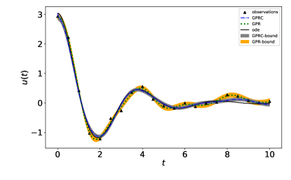
Figure 1: The posterior of the state function $u$. The black triangles represent the $21$ observation data. The black solid curve represents the true solution computed by ODE solver. The blue dash-dot/green dotted traces are the inferred posterior means by GPRC and GPR methods, respectively. The confidence bounds of one posterior standard deviation are also shown.

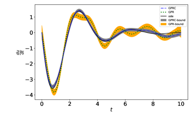
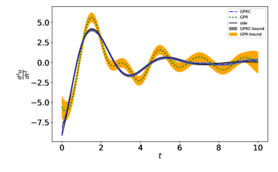
Figure 2: The posterior of the first (left) and second (right) order derivatives. The black curves represent the true solutions. The blue dash-dot/green dotted traces are the inferred posterior means by GPRC and GPR methods, respectively.

In our experiment, there are $21$ observations contaminated by the additive Gaussian noise with zero-mean and variance $\bar{\sigma}_{u}^{2}=0.01$. We set the parameter for the equation constraint $\sigma^{2}_{r}=0.1$. In the prediction, for each $t_{*}$, the extended set $\chi$ is chosen as $60$ points equally spaced in its neighbour $[t_{*}-3,t_{*}+3]$. Figure 1 and 2 show the posteriors of the state and its derivatives in comparison between GPRC and GPR methods. The numerical solution from the ODE solver is regarded as the true solution. The results show that the estimations of all three functions from the GPRC method are much closer to the true solution than the traditional GPR and demonstrate a great ability to correct the model from the noisy observations with the consideration of equation information. Besides, the GPRC gives a greater extent to the variance reduction of the posteriors estimation since the additional observations from the equation constraint $\bm{r}$ in the training and $\bm{r}_{\chi}$ in the prediction are both used.

To examine the effectiveness of our method of incorporating the equation, Figure 3 shows the residual function $r(t)=\mathcal{L}{u}(t)$ where all derivatives in $\mathcal{L}u$ are the mean function of the estimations from GPRC and GPR. We see from this figure that the GPRC with the Product of Experts method in Section 4 show an overall smallness for the residuals. For a quantitative comparison, Table 1 presents the Root Mean Square Error (RMSE) values computed by the posterior mean functions $u$, $u^{\prime}$, $u^{\prime\prime}$ and $r$ with different data noise levels. This confirms the better accuracy of GPRC method with a proper choice of $\sigma_{r}^{2}$. We also tested the effect of the hyper-parameter $\sigma_{r}^{2}$ in the GPRC method by comparing three different values $\sigma_{r}^{2}$ in this table. It is found that a very large value of $\sigma_{r}^{2}$ simply reduces GPRC back to GPR and a smaller $\sigma_{r}^{2}$ does not always help reduce the RMSE, which is consistent with our interpretation of the regularization effect of $\sigma_{r}^{2}$. Recall $\sigma_{r}^{2}$ in the matrix $\sigma_{r}^{2}\bm{I}_{r}$ is used as a regularization for the covariance matrix $K_{rr}$ of the residual $r$. The introduction of this non-zero factor $\sigma_{r}^{2}$ is a beneficial regularization technique. Empirically, we find $\sigma_{r}^{2}\approx 10\sigma_{u}^{2}$ sounds a good choice where $\sigma_{u}^{2}$ can be first approximated from the traditional GPR.

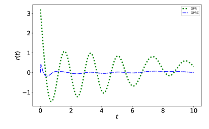
Figure 3: The constraint value computed with posterior means by GPR (green dotted line) and GPRC (blue dash-dot line) method respectively.

Table 1: RMSE of the posterior mean of state, first derivative, second derivative and residual computed by GPR and GPRC when measurement noise with different variances is injected to the measurement data. $\sigma_{r}^{2}$ is the hyper-parameter in GPRC.

noise variance: $0.1$	$u$	$u^{\prime}$	$u^{\prime\prime}$	$r$
GPR	0.36	0.93	3.32	2.09
GPRC($\sigma_{r}^{2}=1e{-3}$)	0.28	0.39	0.75	0.69
GPRC($\sigma_{r}^{2}=1e{-1}$)	0.15	0.20	0.44	0.38
GPRC($\sigma_{r}^{2}=1e{2}$)	0.35	0.91	3.20	1.93
noise variance: $0.05$
GPR	0.16	0.40	2.13	1.28
GPRC($\sigma_{r}^{2}=1e{-3}$)	0.20	0.25	0.55	0.49
GPRC($\sigma_{r}^{2}=1e{-1}$)	0.14	0.17	0.41	0.36
GPRC($\sigma_{r}^{2}=5e{-1}$)	0.11	0.16	0.60	0.37
GPRC($\sigma_{r}^{2}=1e{2}$)	0.16	0.41	1.89	1.12

It is worth noting that too many constraint points is not necessary in prediction process. This viewpoint can be easily verified in this example, shown in Figure 4. In prediction, we select the constraint points in domain $[t_{*}-width,t_{*}+width]$ with spacing $step$, i.e. $t_{*}=2$, $width=1$ and $step=0.5$, then the constraint points are $\{1,1.5,2,2.5,3\}$. Figure 4 Left shows the prediction accuracy would tend to constant with the smaller $step$ values. Same tendency occurs in the Figure 4 right, one with respect to the bigger $width$ values. Both figures illustrate one criterion: the prediction ability would not improve with more constraint points, which is an advantage for the computation complexity of GPRC in Eq.(3.14)-(3.17).

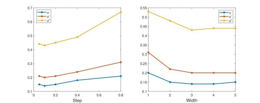
Figure 4: RMSE values of $u$, $u^{\prime}$ and $u^{\prime\prime}$ with respect to different $step$ and $width$. Left: $width=3$ and Right: $step=0.1$.

5.2 Poisson equation

Poisson equation describes the spatial variation of a potential function for given source terms and have important applications in electrostatics and fluid dynamics. Our setting of Poisson equation is as follows

$$\begin{split}\nabla^{2}_{x}u({\bm{x}})&=g(\bm{x}),\\ g(\bm{x})&=\exp(-x_{1})(x_{1}-2+x^{3}_{2}+6x_{2}),\end{split}$$ (5.2)

with Dirichlet boundary conditions

$$\begin{split}u(0,x_{2})&=x^{3}_{2},\\ u(1,x_{2})&=(1+x^{3}_{2})\exp(-1),\\ u(x_{1},0)&=x_{1}\exp(-x_{1}),\\ u(x_{1},1)&=(x_{1}+1)\exp(-x_{1}),\end{split}$$ (5.3)

and the domain is $[0,1]\times[0,1]$. The analytic solution is

$$u({\bm{x}})=\exp(-x_{1})(x_{1}+x_{2}^{3}).$$

This PDE corresponds to the zero value of the residual $r:=\frac{\partial^{2}u}{\partial x_{1}^{2}}+\frac{\partial^{2}u}{\partial x_{2}^{2}}-g$. Assume the state is a Gaussian process as (3.1), and then the constraint is also a Gaussian process which is written as $r({\bm{x}})\sim\mathcal{N}(0,k_{r})$, where $k_{r}=k_{u_{1}^{\prime\prime}u_{1}^{\prime\prime}}+k_{u_{2}^{\prime\prime}u_{2}^{\prime\prime}}+k_{u_{2}^{\prime\prime}u_{1}^{\prime\prime}}+k_{u_{1}^{\prime\prime}u_{2}^{\prime\prime}}$. The boundary conditions of $u$ and $\frac{\partial^{2}u}{\partial x_{2}^{2}}$ can be easily obtained by Poisson equation (5.2) and Dirichlet BCs (5.3).

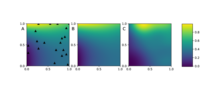
Figure 5: A: The black triangles represent the positions of the observation data and the contour plot of the true solution $u({\bm{x}})$. B and C show the posterior mean of state computed by GPRC and GPR, respectively.

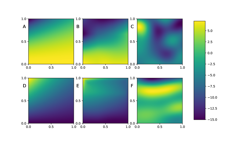
Figure 6: The first and second rows represent the estimation of $\frac{\partial^{2}u}{\partial x_{1}\partial x_{2}}$ and $\frac{\partial^{2}u}{\partial x_{2}^{2}}$, respectively. A and D show the analytical solutions. B and E represent the posterior means estimated by GPRC. C and F represent the posterior means estimated by GPR.

$15$ observations of $u$ at $15$ locations in the square domain were measured as shown in Figure 5 with additive noise with the variance $\sigma_{u}^{2}=0.01$. Here we set the slack parameter $\sigma^{2}_{r}=0.3$. The extended set $\chi$ in the neighbourhood of a test point ${\bm{x}}_{*}$ is composed of $5\times 5$ points equally spaced in square domain $[x_{*1}-0.33,x_{*1}+0.33]\times[x_{*2}-0.33,x_{*2}+0.33]$. Figure 5 also shows the posterior mean functions of the state $u$ estimated by GPRC and GPR, respectively. Figure 6 shows the posterior mean functions of the second order derivatives $\frac{\partial^{2}u}{\partial x_{1}\partial x_{2}}$ and $\frac{\partial^{2}u}{\partial x_{2}^{2}}$, respectively. The predictions of these derivatives by GPRC are much better than the ones by the GPR method. Table 2 shows the RMSE of the posterior mean of state and second derivatives computed by GPR and GPRC respectively. The RMSE values of GPRC is much smaller than the ones computed by GPR, which indicates the advantage of modeling with constraint information.

Table 2: RMSE for the Poisson equation

		$u$		$\frac{\partial^{2}u}{\partial x_{1}\partial x_{2}}$		$\frac{\partial^{2}u}{\partial x_{2}^{2}}$
GPR		0.0720		1.91		4.71
GPRC		0.0067		0.26		0.32

5.3 Van der Pol equation

Van der Pol equation is a typical nonlinear ODE which can generate shock wave solution. It is defined as

$$\frac{d^{2}u}{dt^{2}}-\mu(1-u^{2})\frac{du}{dt}+u=0,$$ (5.4)

where $\mu=0.5$ and the initial conditions are $u(0)=2,u^{\prime}(0)=0$. We can’t directly make use of GPRC method to formulate the residual of (5.4) as an aforementioned Gaussian process $r$, since the product of Gaussian processes is not a Gaussian process anymore. Here we propose an iteratively linearization method for nonlinear equations, motivated by the Picard iteration method[5]. Assume we have an initial guess of the solution $u_{0}$, then we can rewrite the equation (5.4) as:

$$\frac{d^{2}u}{dt^{2}}-\mu(1-u_{0}^{2})\frac{du}{dt}+u=0,$$ (5.5)

where the original $u$ in the nonlinear coefficient term is replaced by $u_{0}$. Now (5.5) is a linear equation of $u$ and GPRC can be directly applied to estimate the solution $u$ and its derivatives $u^{\prime},u^{\prime\prime}$. The constraint variable for (5.5) is then expressed as $r_{0}=\frac{d^{2}u}{dt^{2}}-\mu(1-u_{0}^{2})\frac{du}{dt}+u$ and the corresponding value is $0$. This is a quite straightforward linearlization strategy and can be easily applied to most non-linear differential equations. The initial solution guess $u_{0}$ can be roughly estimated by the classical GPR (or any other data smoothing method) from observations of $u$. The new estimation of $u$ from GPRC then serves as a new $u_{0}$ in (5.4) in a recursive way. The number of such iterations depends on the quality of learning initial $u_{0}$ from data, the specific linearization form of (5.5), and the convergence of Picard iteration. So it is problem-dependent, but as a practical tool, this strategy is easy to implement and in some cases it only takes one or two iterations in practice, as shown numerically below in the nonlinear Van der Pol oscillator.

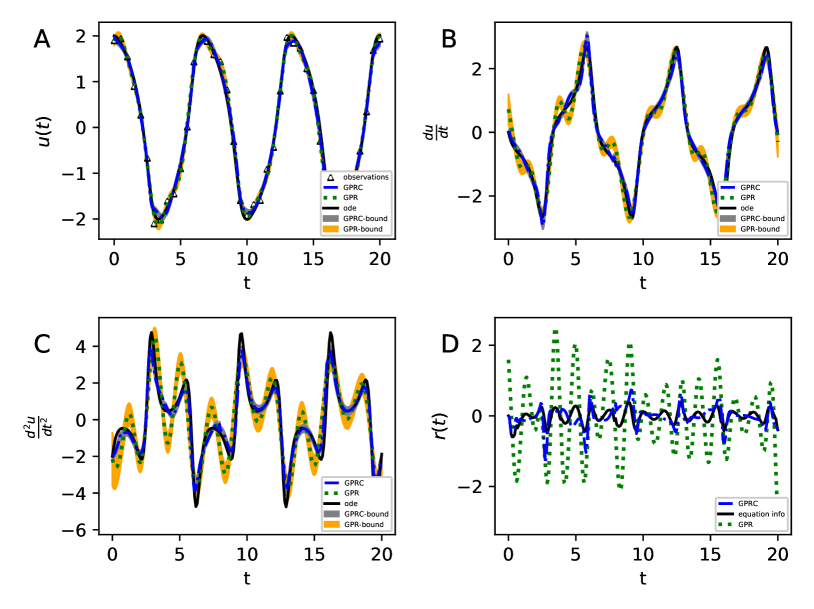
Figure 7: (Van der Pol equation.) A, B and C: The triangles represent the observed data-points of the noisy process. The black line shows the true solution (computed by the ODE solver). The blue dash-dotted annd green dotted lines are, respectively, the inferred posterior means by GPRC and GPR method with a confidence band of $\pm$ one posterior standard deviation. D: The black line shows the residual $r_{0}$ of the linearlization equation (5.5). The blue dash-dotted and the green dotted lines are the true (nonlinear residual) in (5.4) computed on the posterior means respectively by GPRC and GPR.

40 observations are measured with equal space in the time interval $[0,20]$, contaminated by the additive Gaussian noise with variance $\sigma^{2}_{u}=0.01$. The extend set $\chi$ for each test point $x_{*}$ is chosen as $4$ points equally spaced in $[x_{*}-0.2,x_{*}+0.2]$ and the hyper-parameter $\sigma^{2}_{r}=0.1$. The initial $u_{0}$ is from GPR with the given $40$ observations. Here we only take one iteration of Picard approximation to obtain a very good result and we found more iterations did not improve the posterior estimation further. Figure 7 compares the result from GPR and GPRC. Although both methods perform well on the estimation of the state variable $u$, for the first order derivative function, the GPR method starts to show spurious small oscillations and for the second order derivative, the GPR method produces the erratic phase and amplitude. By contrast, the GPRC method gives a consistent and robust posterior prediction for the derivatives from zero order to second order. Note that GPRC here did not solve the Van del Pol equation on the whole interval $[0,20]$ and the extended set $\chi$ only has a width $0.6$.

Panel D of Figure 7 further shows the residual $r_{0}$ of the linearized equation (black line) and the true $r$ of the Van der Pol equation (blue line), which confirms that just one Picard iteration in this example has achieved quite good results. The RMSE (Root Mean Square Error) of the nonlinear constraint $r$ with increased measurement noise variances are summarized in Table 3 and illustrates the trend of convergence of the GPRC algorithm with only one Picard iteration.

Table 3: (Van der Pol equation) The RMSE of the true (nonlinear) residual $r$ based on the mean function from GPRC with observation contaminated by different noise variances.

noise variance		0.10		0.05		0.01
RMSE		0.0128		0.0094		0.0079

5.4 Application to identify the parameter $\mu$

We continue to consider the Van del Pol model and explain how the robust estimation of derivatives by GRPC can help improve the method for the problem of parameter identification $\mu$ . Our previous numerical results are all associated with a given parameter $\mu=0.5$ in (5.4). We denote this ground truth as $\mu^{\star}=0.5$ and make $\mu$ a generic variable. Let $(t_{i},y_{i})$ be $n$ given observations of $u(t)$ on the given location $t_{i}$. The general methodology [23, 3, 17] is to estimate a function $\widehat{u}(t)$ first from the data, for instance, by minimizing the sum-of-squared loss $\sum_{i}|y_{i}-\widehat{u}_{i}|^{2}$ where $\widehat{u}_{i}=\widehat{u}(t_{i})$ and then to find the optimal parameter $\mu$ by minimizing the squared error of the equation’s residual $\sum_{j}|r_{j}|^{2}$ on a set of $m$ design points $\{\widehat{t}_{j}\}$ (which can be either the same as the original measurement locations or a new set with $m>n$). We can write the sum of two losses as follows (with the equal weight for both losses for simplicity):

$$L_{loss}(\mu)=\frac{1}{n}\sum_{i=1}^{n}(y_{i}-\widehat{u}_{i})^{2}+\frac{1}{m}\sum_{j=1}^{m}\bigg{(}\widehat{\frac{d^{2}u_{j}}{dt^{2}}}-\mu(1-\widehat{u}_{j}^{2})\widehat{\frac{du_{j}}{dt}}+\widehat{u}_{j}\bigg{)}^{2}.$$ (5.6)

The key issue here in our focus is the computation of derivatives in the second part: $\widehat{\frac{du_{j}}{dt}}$, $\widehat{\frac{d^{2}u_{j}}{dt^{2}}}$ are just $\frac{d}{dt}\widehat{u}(t)$ and $\frac{d^{2}}{dt^{2}}\widehat{u}(t)$ at $t=\widehat{t}_{j}$ or estimated alternatively. The traditional method, such as GPR, estimates $\widehat{u}(t)$ only based on the data $(t_{i},y_{i})$, and the derivatives in (5.6) are the numerical or analytical differentials of $\widehat{u}$. So the obtained function $\widehat{u}$ is independent of $\mu$ and (5.6) is exactly a quadratic function of $\mu$ for this example (the first term has no effect in identifying $\mu$). However, when our GPRC is applied to this problem, for each $\mu$, we use the data $(t_{i},y_{i})$ and the equation associated with this postulated $\mu$ to jointly estimate $\widehat{u}(t)$, $\widehat{\frac{du}{dt}}(t)$ $\widehat{\frac{d^{2}u}{dt^{2}}}(t)$ to compute $L_{loss}(\mu)$ and consequently, all hatted terms in (5.6) $L_{loss}(\mu)$ depend on $\mu$ and $L_{loss}(\mu)$ no longer has a simple quadratic expression. The optimal $\mu$ is then the minimizer of this $L_{loss}(\mu)$. In summary, the application of GPRC for parameter identification problem, conceivably, is to solve $\displaystyle\min_{\mu}\min_{\widehat{u},\widehat{u^{\prime}},\widehat{u^{\prime\prime}}}L_{loss}(\mu;\{t_{i},y_{i}\})$ where the $\min$ inside is the GPRC.

To demonstrate the importance of getting the right estimation of derivatives used in the loss function $L_{loss}$, Figure 8 shows the values of $L_{loss}$ with respect to the parameter $\mu$. Note the ground truth $\mu^{\star}=0.5$. With the same $n=40$ observations, the minimizer in the first subplot corresponding to GPRC can recover this parameter between $0.4\sim 0.5$, while the minimizer in the middle subplot corresponding to GPR gives a completely wrong answer because the derivatives used are not as accurate and robust as from GPRC even at the true $\mu^{\star}$. If we are able to use a large number of observations of $u$, say $n=400$ in the right subplot of Figure 8, the traditional GPR is then capable to find the correct optimal parameter $\mu^{\star}$. So, the traditional method like GPR method to estimate the function $\widehat{u}(t)$ only and to rely on numerical/analytical differentiation of $\widehat{u}(t)$ works only if the number of observations is sufficiently large. The benefit of the new GPRC method advocated here has a potential advantage when the available data points are limited.

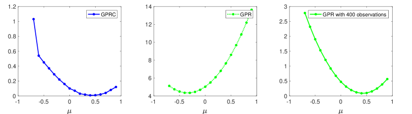
Figure 8: Left and Middle: $L_{loss}$ in (5.6) with respect to the parameter $\mu$, computed by GPRC (left) and GPR (middle), respectively, based on the same measurements on 40 locations in Section 5.3. Right: $L_{loss}$ with respect to the parameter $\mu$, computed by GPR from a larger dataset of $400$ observations.

6 Conclusions

In this work, we have shown how to improve the accuracy and robustness for the numerical estimation of derivatives from the noisy state data by our new method of Gaussian process regression with constraint (GPRC) for linear and nonlinear differential equations. Explicit posteriors with uncertainty information are obtained in the Bayesian framework for the joint multi-dimensional GPR. For nonlinear differential equations, a strategy of linearization method motivated from the Picard iteration is applied. From the perspective of incorporating the differential equations into the Gaussian process regression (GPR), our work is a kind of physics-informed Gaussian process regression, compatible with the recent awareness of the importance of combining the observations of solution data and the underlying physical model [14].

An important toy example of Van de Pol equation has been presented to show, when applied to the parameter identification problem, the joint estimation of the solution and its derivatives by our new method make an important contribution to identifying the missing parameter correctly with fewer samples. The method developed here may have a potential application for the more complication problems like parameter identification [17]. It is foreseen that the price to pay could be the extra optimization costs since all terms in $L_{loss}(\mu)$ in (5.6) involve the unknown parameter $\mu$. It would be interesting to develop certain fast sequential methods to improve the efficiency for such problems.

So far, the equations we have considered are deterministic with known or missing coefficients, and the hyper-parameter parameter $\sigma_{r}^{2}$ is beneficial in practice as regularization to allow some prior distribution for the zero residual. For the stochastic differential equations with random coefficients, one may include this uncertainty of residual into the likelihood function in the same Bayesian framework; however with the restriction of Gaussian assumption, the approach of GPR may not be applicable except in some special cases in [15].

References

- [1] David Barber and Yali Wang. Gaussian processes for Bayesian estimation in ordinary differential equations. In International Conference on Machine Learning, pages 1485–1493, 2014.
- [2] F. Brezzi. A survey of mixed finite element methods. In D. L. Dwoyer, M. Y. Hussaini, and R. G. Voigt, editors, Finite Elements, pages 34–49, New York, NY, 1988. Springer New York.
- [3] Steven L. Brunton, Joshua L. Proctor, J. Nathan Kutz, and William Bialek. Discovering governing equations from data by sparse identification of nonlinear dynamical systems. Proc. Natl. Acad. Sci. U. S. A., 113(15):3932–3937, 2016.
- [4] Ben Calderhead, Mark Girolami, and Neil D Lawrence. Accelerating Bayesian Inference over Nonlinear Differential Equations with Gaussian Processes. In Advances in Neural Information Processing Systems, 2009.
- [5] Earl A Coddington and Norman Levinson. Theory of Ordinary Differential Equations. Tata McGraw-Hill Education, 1955.
- [6] Jianqing Fan and Irène Gijbels. Local Polynomial Modelling and its Applications. Chapman & Hall, London, 1996.
- [7] Pei Gao, Antti Honkela, Magnus Rattray, and Neil D. Lawrence. Gaussian process modelling of latent chemical species: applications to inferring transcription factor activities. Bioinformatics, 24(16):i70–i75, 08 2008.
- [8] Thore Graepel. Solving noisy linear operator equations by Gaussian process: Application to ordinary and partial differential equations. In International Conference on Machine Learning, pages 234–241, 2003.
- [9] T. Hastie, R. Tibshirani, and J.H. Friedman. The Elements of Statistical Learning: Data Mining, Inference, and Prediction. Springer, second edition, 2009.
- [10] Hua Liang and Hulin Wu. Parameter estimation for differential equation models using a framework of measurement error in regression models. Journal of the American Statistical Association, 103(484):1570–1583, 2008.
- [11] Guy Mayraz and Geoffrey E Hinton. Recognizing hand-written digits using hierarchical products of experts. In Advances in Neural Information Processing Systems, pages 953–959, 2001.
- [12] AA Poyton, M Saeed Varziri, Kim B McAuley, P James McLellan, and Jim O Ramsay. Parameter estimation in continuous-time dynamic models using principal differential analysis. Computers & Chemical Engineering, 30(4):698–708, 2006.
- [13] Maziar Raissi and George Em Karniadakis. Hidden physics models: Machine learning of nonlinear partial differential equations. Journal of Computational Physics, 357:125–141, 2018.
- [14] Maziar Raissi, Paris Perdikaris, and George E Karniadakis. Physics-informed neural networks: A deep learning framework for solving forward and inverse problems involving nonlinear partial differential equations. Journal of Computational Physics, 378:686–707, 2019.
- [15] Maziar Raissi, Paris Perdikaris, and George Em Karniadakis. Machine learning of linear differential equations using Gaussian processes. Journal of Computational Physics, 348:683–693, 2017.
- [16] J. O. Ramsay, G. Hooker, D. Campbell, and J. Cao. Parameter estimation for differential equations: A generalized smoothing approach. J. R. Stat. Soc. Ser. B Stat. Methodol., 69(5):741–796, 2007.
- [17] Samuel H Rudy, Steven L Brunton, Joshua L Proctor, and J Nathan Kutz. Data-driven discovery of partial differential equations. Science Advances, 3(4):e1602614, 2017.
- [18] Simo Särkkä. Linear operators and stochastic partial differential equations in Gaussian process regression. In International Conference on Artificial Neural Networks, pages 151–158. Springer, 2011.
- [19] Matthias Seeger. Gaussian processes for machine learning. International Journal of Neural Systems, 14(02):69–106, 2004.
- [20] Peter S Swain, Keiran Stevenson, Allen Leary, Luis F Montano-Gutierrez, Ivan BN Clark, Jackie Vogel, and Teuta Pilizota. Inferring time derivatives including cell growth rates using processes. Nature communications, 7:13766, 2016.
- [21] Vladimir N. Vapnik. Statistical Learning Theory. Wiley-Interscience, 1998.
- [22] James M Varah. A spline least squares method for numerical parameter estimation in differential equations. SIAM Journal on Scientific and Statistical Computing, 3(1):28–46, 1982.
- [23] Xiaolei Xun, Jiguo Cao, Bani Mallick, Arnab Maity, and Raymond J Carroll. Parameter estimation of partial differential equation models. Journal of the American Statistical Association, 108(503):1009–1020, 2013.