The QCD critical point from the Nambu-Jona-Lasino model with a scalar-vector interaction

Abstract

We study the critical point in the QCD phase diagram in the Nambu-Jona-Lasino (NJL) model by including a scalar-vector coupled interaction. We find that varying the strength of this interaction, which has no effect on the vacuum properties of QCD, can significantly affect the location of the critical point in the QCD phase diagram, particularly the value of the cirtical temperature. This provides a convenient way to use the NJL-based transport or hydrodynamic model to extract information about the QCD phase diagram from relativistic heavy-ion collisions.

I Introduction

Studying the QCD phase structure is among the most important goals of ongoing experiments on heavy-ion collisions Braun-Munzinger et al. (2016); Luo and Xu (2017); Bzdak et al. (2019). By changing the beam energy and selecting different system sizes and the rapidities of measured particles, it is possible to probe different regions of the QCD phase diagram, particularly the critical endpoint (CEP) Stephanov (2006) on the first-order phase transition line. To make this possible requires, however, versatile dynamic models to describe the expansion of created hot dense matter with a flexible equation of state that can have the critical point at varying temperatures ($T$) and baryon chemical potentials ($\mu_{B}$) in the QCD phase diagram Nahrgang (2015); Bluhm et al. (2020); Murase and Hirano (2016); Hirano et al. (2019); Nahrgang et al. (2017); Bluhm et al. (2018); Singh et al. (2019); Akamatsu et al. (2017); An et al. (2019); Stephanov and Yin (2018); Rajagopal et al. (2019).

At zero and small baryon chemical potentials, the lattice quantum chromodynamics (LQCD) Bernard et al. (2005); Aoki et al. (2006); Bazavov et al. (2012) has shown that the quark-gluon plasma (QGP) to hadronic matter phase transition is a smooth crossover. Although it is not yet possible for the lattice QCD to study the quark-hadron phase transition at high baryon chemical potential due to the fermion sign problem. Studies based on effective theories have suggested that the phase transition is a first-order one at large baryon chemical potential Asakawa and Yazaki (1989); Fukushima (2008); Carignano et al. (2010); Bratovic et al. (2013); Stephanov (2004, 2006); Fukushima and Sasaki (2013); Baym et al. (2018), indicating the existence of a CEP on the first-order phase transition line in the $\mu_{B}-T$ plane of the QCD phase diagram. However, its predicted location has large uncertainties and even its existence remains unclear Stephanov (2004).

Among the effective models for studying the QCD phase diagram at finite baryon chemical potential, a frequently used one is the Nambu-Jona-Lasinio model Nambu and Jona-Lasinio (1961a, b). Formulated in terms of quark degrees of freedom Eguchi (1976); Kikkawa (1976), this model allows the description of chiral phase transition at both finite temperature and chemical potential Buballa (2005a) besides providing a framework to describe hadronic systems in the vacuum based on dynamical chiral symmetry breaking and its restoration Vogl and Weise (1991a); Klevansky (1992); Hatsuda and Kunihiro (1994). The improved NJL model with the Polyakov-loop (PNJL) also makes it possible to describe the confinement-deconfinement phase transition of the quark matter Meisinger and Ogilvie (1996); Meisinger et al. (2002, 2004); Fukushima (2004); Mocsy et al. (2004); Ratti et al. (2006); Roessner et al. (2007); Fukushima (2008). The parameters in the NJL model and the PNJL model are largely constrained by the vacuum properties of QCD and the known chiral dynamics in hadron systems at zero temperature. The predicted temperature of the critical point in the NJL model varies from 40 to 80 MeV Stephanov (2004); Buballa (2005a), while its value in the PNJL model can be larger than 100 MeV Roessner et al. (2007); Costa et al. (2010). For the purpose of locating the critical point via comparing model calculations with the experimental data from heavy-ion collisions, it will be useful to extend the NJL-type models to further expand the region in the $\mu_{B}-T$ plane where possible locations of the critical point can be accommodated.

Although a repulsive vector interaction can be included in the NJL or PNJL model to change the critical temperature of the chiral and/or deconfinement phase transition Fukushima (2008), it, however, leads to a decrease of the critical temperature, making the deviation from the LQCD results even larger Steinheimer and Schramm (2014). Another way to extend the NJL model is to include higher-order multi-quark interactions. Besides the six-quark interaction term from the ’t Hooft determinant interaction that breaks the $U_{A}(1)$ symmetry ’t Hooft (1976), the eight-quark interactions including scalar-scalar, vector-vector, and scalar-vector coupled interaction terms have also been considered Kashiwa et al. (2007); Osipov et al. (2006a, b). These higher-order interactions are produced from quantum effects in the high momentum region of the nonperturbative renormalization group calculation Aoki et al. (2000). Since the attractive scalar-scalar coupled interaction affects the QCD vacuum properties, its strength is constrained and can not be arbitrarily changed to modify the location of the critical point. Although the repulsive vector-vector coupled interaction does not affect the QCD vacuum properties, it always decreases the critical temperature of baryon-rich quark matter, similar to the effect due to the vector interaction. For the scalar-vector coupled interaction, it is known to be important for reproducing the nuclear saturation properties when using the NJL-type model for nuclear matter Koch et al. (1987). As to its application to the quark-hadron phase transition Lee et al. (2013), it turns out to be a good candidate because it has no effects on the QCD vacuum properties, and more importantly, its strength can affect the location of the critical point as to be shown below. By tuning the coupling constant of the scalar-vector coupled interaction, we can easily change the location of the critical point in the phase diagram from low to very high temperatures. These features of the scalar-vector coupled interaction term were not fully appreciated in previous studies Kashiwa et al. (2007); Osipov et al. (2006a, b).

In the present work, we first calculate the phase diagram from the two-flavor NJL model by including the scalar-vector coupled interaction among quarks. We then extend the calculations to the three-flavor case and also to the PNJL model to study in detail its effect on the location of the critical point in the QCD phase diagram.

II The Scalar-Vector coupled interaction in the (P)NJL model

II.1 The two-flavor NJL model

We begin by considering the two-flavor NJL model that is usually described by the following Lagrangian density Buballa (2005a),

$$\mathcal{L}_{\text{NJL}}^{\text{SU(2)}} = \mathcal{L}_{0}+\mathcal{L}_{\text{S}}+\mathcal{L}_{\text{SV}},$$ (1)

with

$$\mathcal{L}_{0}=\bar{\psi}(i\gamma^{\mu}\partial_{\mu}-\hat{m})\psi,$$

$$\mathcal{L}_{\text{S}}=G_{S}[(\bar{\psi}\psi)^{2}+(\bar{\psi}i\gamma_{5}\vec{\tau}\psi)^{2}],$$

$$\mathcal{L}_{\text{SV}}=G_{SV}[(\bar{\psi}\psi)^{2}+(\bar{\psi}i\gamma_{5}\vec{\tau}\psi)^{2}]$$

$$\qquad\quad\times[(\bar{\psi}\gamma^{\mu}\psi)^{2}+(\bar{\psi}\gamma_{5}\gamma^{\mu}\vec{\tau}\psi)^{2}].$$ (2)

In the above, $\psi=(u,d)^{T}$ represents the 2-flavor quark fields, $\hat{m}=\text{diag}(m_{u},m_{d})$ is the current quark mass matrix, $\gamma^{\mu}$ and $\gamma_{5}=i\gamma_{0}\gamma_{1}\gamma_{2}\gamma_{3}$ are Dirac matrices, and $\vec{\tau}=(\tau_{1},\tau_{2},\tau_{3})$ is the Pauli matrices in the flavor space. The Lagrangian densities $\mathcal{L}_{0}$, $\mathcal{L}_{\text{S}}$, and $\mathcal{L}_{\text{SV}}$ are, respectively, for the free quarks and their scalar and pseudoscalar interactions with the coupling constant $G_{S}$ as well as the scalar-vector, scalar-axial vector, pseudoscalar-vector and pseudoscalar-axial vector coupled interactions with the coupling constant $G_{SV}$. We note that the sign of the $G_{SV}$ term in Eq. (2) is the same as the original one introduced in Ref. Koch et al. (1987), which is opposite to that used in Refs. Kashiwa et al. (2007); Lee et al. (2013).

As in most studies using the NJL model, we adopt the mean-field approximation Vogl and Weise (1991b) to linearize the model by introducing the following substitutions,

$$(\bar{\psi}\Gamma_{i}\psi)^{2} = 2\bar{\psi}\Gamma_{i}\psi\langle\bar{\psi}\Gamma_{i}\psi\rangle-\langle\bar{\psi}\Gamma_{i}\psi\rangle^{2}$$

$$(\bar{\psi}\Gamma_{i}\psi\bar{\psi}\Gamma_{j}\psi)^{2} = \langle\bar{\psi}\Gamma_{i}\psi\rangle^{2}(2\bar{\psi}\Gamma_{j}\psi\langle\bar{\psi}\Gamma_{j}\psi\rangle)$$ (3)

$$+\langle\bar{\psi}\Gamma_{j}\psi\rangle^{2}(2\bar{\psi}\Gamma_{i}\psi\langle\bar{\psi}\Gamma_{i}\psi\rangle)$$

$$-3\langle\bar{\psi}\Gamma_{i}\psi\rangle^{2}\langle\bar{\psi}\Gamma_{j}\psi\rangle^{2},$$

where $\Gamma=\{1,i\gamma_{5}\vec{\tau},\gamma_{\mu},\gamma_{5}\gamma_{\mu}\}$ and the angular bracket denotes the expectation value from the quantum-statistical average. Due to the parity symmetry in a static quark matter, one has $\langle\bar{\psi}\gamma^{k}\psi\rangle=\langle\bar{\psi}\gamma_{5}\vec{\tau}\psi\rangle=\langle\bar{\psi}\gamma_{5}\gamma^{\mu}\psi\rangle=0$, and the Lagrangian density can then be rewritten as

$$\mathcal{L}_{\text{NJL}}^{\text{SU(2)}}=\bar{u}(\gamma^{\mu}i\partial_{u\mu}-M_{u})u+\bar{d}(\gamma^{\mu}i\partial_{d\mu}-M_{d})d$$

$$\quad+2G_{SV}(\rho_{u}+\rho_{d})(\phi_{u}+\phi_{d})^{2}(\bar{u}\gamma^{0}u+\bar{d}\gamma^{0}d)$$

$$\quad-G_{S}(\phi_{u}+\phi_{d})^{2}-3G_{SV}(\phi_{u}+\phi_{d})^{2}(\rho_{u}+\rho_{d}),$$ (4)

In the above, $M_{u}$ and $M_{d}$ are the in-medium effective masses of $u$ and $d$ quarks, respectively, given by

$$M_{u} = m_{u}-2G_{S}(\phi_{u}+\phi_{d})$$

$$- 2G_{SV}(\rho_{u}+\rho_{d})^{2}(\phi_{u}+\phi_{d}),$$

$$M_{d} = m_{d}-2G_{S}(\phi_{u}+\phi_{d})$$ (5)

$$- 2G_{SV}(\rho_{u}+\rho_{d})^{2}(\phi_{u}+\phi_{d}),$$

with $\phi_{u}=\langle\bar{u}u\rangle$ and $\phi_{d}=\langle\bar{d}d\rangle$ being the $u$ and $d$ quark condensates, respectively, and $\rho_{u}$ and $\rho_{d}$ denoting the net $u$ and $d$ quark number densities, respectively.

The thermodynamic properties of a two-favour quark matter are determined by the partition function $\mathcal{Z}=\text{Tr}[\exp[-\beta(\hat{H}-\mu\hat{N})]]$, where $\beta=1/T$ and $\hat{H}$ are, respectively, the inverse of the temperature $T$ and the Hamiltonian operator, and $\mu$ and $\hat{N}$ are, respectively, the chemical potential and corresponding conserved charge number operator. The thermodynamic grand potential of the system is then given by

$$\Omega_{\text{NJL}}^{\text{SU(2)}}=-\frac{1}{\beta V}\text{ln}\mathcal{Z}$$ (6)

$$\qquad=G_{S}(\phi_{u}+\phi_{d})^{2}+3G_{SV}(\phi_{u}+\phi_{d})^{2}(\rho_{u}+\rho_{d})$$

$$\qquad-2N_{c}\sum_{i=u,d}\int\frac{\text{d}^{3}p}{(2\pi)^{3}}E_{i}$$

$$\qquad-2T\sum_{i=u,d}\int\frac{\text{d}^{3}p}{(2\pi)^{3}}(z^{+}(E_{i})+z^{-}(E_{i})),$$

where $V$ is volume of the system, $N_{c}=3$ is the number of colors, $E_{i}=(m_{i}^{2}+{\bf p}^{2})^{1/2}$, and

$$z^{\pm}(E_{i}) = N_{c}\text{ln}[1+\text{e}^{-\beta(E_{i}\mp\mu_{i}^{*})}].$$ (7)

with the effective chemical potentials,

$$\mu_{u}^{*} = \mu_{u}+2G_{SV}(\rho_{u}+\rho_{d})(\phi_{u}+\phi_{d})^{2},$$

$$\mu_{d}^{*} = \mu_{d}+2G_{SV}(\rho_{u}+\rho_{d})(\phi_{u}+\phi_{d})^{2}.$$ (8)

Table 1: Parameters in the two-flavor NJL model Ratti et al. (2006); Roessner et al. (2007).

$\Lambda$ [MeV]	$G_{S}\Lambda^{2}$	$m_{u,d}$ [MeV]	$M_{u,d}$ [MeV]	$\langle\bar{u}u\rangle^{1/3}$ [MeV]
651	2.135	5.5	325.1	-251.3

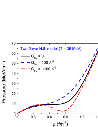
Figure 1: (Color online) Pressure as a function of net quark number density at temperature $T=36$ MeV from the two-flavor NJL model for different values of the scalar-vector coupling constant $G_{SV}$ and with the values of other parameters given in Table 1.

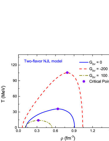
Figure 2: (Color online) Coexistence lines in the temperature and net quark number density plane from the two-flavor NJL model for different values of the scalar-vector coupling constant $G_{SV}$ and with the values of other parameters given in Table 1. The solid circles denote corresponding critical points.

The quark condensate $\phi_{i}$ and the net quark number density $\rho_{i}$ can be determined by minimizing the grand potential, i.e.,

$$\frac{\partial\Omega_{\text{NJL}}^{\text{SU(2)}}}{\partial\phi_{i}}=\frac{\partial\Omega_{\text{NJL}}^{\text{SU(2)}}}{\partial\rho_{i}}=0,$$ (9)

and they are

$$\phi_{i} = 2N_{c}\int\frac{d^{3}p}{(2\pi)^{3}}\frac{M_{i}}{E_{i}}(n^{+}_{i}+n^{-}_{i}-1),$$ (10)

$$\rho_{i} = 2N_{c}\int\frac{d^{3}p}{(2\pi)^{3}}(n^{+}_{i}-n^{-}_{i}),$$ (11)

with $n^{\pm}_{i}=[e^{\beta(E_{i}\mp\mu_{i}^{*})}+1]^{-1}$. Because the NJL model is unrenormalizable, a momentum cutoff $\Lambda$ is needed in evaluating the momentum integral in Eqs. (10) and (11). In the present study, we employ the parameters $m_{u}=m_{d}=5.5$ MeV, $G_{S}\Lambda^{2}=2.135$, and a cut-off $\Lambda=651$ MeV Ratti et al. (2006); Roessner et al. (2007), which are summarized in Table 1 together with the quark in-medium mass and condensate, to study the QCD phase diagram with various values for $G_{SV}$.

With the quark condensates and net quark density given in the above, one can see from Eq. (5) and Eq. (8) that the $G_{SV}$ term affects the effective masses of quarks and their effective chemical potentials in a quark matter. Although its effects depend on the quark condensates, which have negative values and increase with decreasing quark density, they also depend on the quark density. As a result, including the $G_{SV}$ term in the NJL model does not affect its description of QCD vacuum properties at zero baryon density, and treating the value of $G_{SV}$ as a free parameter allows one to obtain different scenarios for the properties of quark matter.

The effects of the $G_{SV}$ term can be qualitatively understood for quark matter at low density. According to Eq.(II.1), a negative $G_{SV}$ resembles a vector interaction in the NJL model Buballa (2005a), which induces a repulsive interaction among quarks or anti-quarks and an attractive interaction between quark and anti-quark. Compared to the scalar coupled term $G_{S}$ in the NJL model, which reduces the quark masses in a medium because of the reduction of quark condensates, a negative $G_{SV}$ counteracts this effect as can be seen from Eq.(5). With its quadratic dependence on the quark density, the effect of the $G_{SV}$ term on the quark in-medium masses at low quark densities is, however, significantly reduced with increasing quark density, thus resulting in an effectively attractive interaction among quarks. Since the repulsive quark interaction due to a negative $G_{SV}$ in the vector channel turns out to be stronger than the attractive quark interaction in the scalar channel for quark matter at low densities, the net effect of a negative $G_{SV}$ is repulsive. In quark matter at very high densities, where the chiral symmetry is largely restored and the quark condensates are thus close to zero, the effects of the $G_{SV}$ term become less important, which is different from the usual vector interaction in the NJL model Buballa (2005a) that gets stronger at high densities. For quark matter at intermediate densities, the effects of the $G_{SV}$ term are, however, more complex, and whether this leads to a repulsive or an attractive quark interaction depends on the value of the quark density. For a positive $G_{SV}$, its effects on the properties of quark matter are opposite to those of a negative $G_{SV}$.

The effects of the $G_{SV}$ term can be quantitatively understood from the pressure of a quark matter, which is given by $p=-\Omega_{\text{NJL}}^{\text{SU(2)}}$, as a function of the net quark number density. In Fig. 1, we show the results for quark matter at temperature $T=36$ MeV for different values of the scalar-vector coupling constant $G_{SV}$. The temperature $T=36$ MeV is the critical temperature in the two-flavor NJL model for $G_{SV}=0$. It is seen that a positive $G_{SV}=$ 100$\Lambda^{-8}$ hardens the equation of state at net quark number density of around 0.9 fm^-3, while a negative $G_{SV}=$ -100$\Lambda^{-8}$ has the opposite effects. As a result, a negative $G_{SV}$ leads to a higher critical temperature while a positive one leads to a lower critical temperature.

Figure 2 shows the coexistence line in the temperature and net quark number density plane for different values of $G_{SV}$. For points on the coexistence line that have same temperature, they are obtained by requiring equal pressure and chemical potential for the two phases with different quark number densities. The region below the coexistence line is unstable with regard to the phase separation. The blue solid line is the result calculated with $G_{SV}$ = 0, i.e., the default NJL model, and the corresponding critical point is located at temperature $T\approx$ 36 MeV and net quark number density $\rho\approx$ 0.64 fm^-3. Results obtained with a scalar-vector coupled interaction of $G_{SV}=$ -200 $\Lambda^{-8}$ are shown by the dashed line, and the critical point in this case shifts to the temperature $T\approx$ 105.5 MeV and net quark density $\rho\approx$ 0.79 fm ^-3. Changing to a scalar-vector coupled interaction of $G_{SV}=$ 100 $\Lambda^{-8}$, reduces the temperature and net quark number density of the critical point to $T\approx$ 14 MeV and $\rho\approx$ 0.32 fm ^-3, respectively. Hence, the critical temperature can be easily increased or decreased by decreasing or increasing the value of $G_{SV}$. For later comparisons of results from the three-flavor NJL model and the NJL model with the Polyakov loop, we also show in Fig. 3 by the red line the locations of the critical point in the temperature and baryon chemical potential plane from the two-flavor NJL model with various values of $G_{SV}$. Although it is not possible to make the critical point approach the $\mu_{B}=0$ axis by further reducing the value of $G_{SV}$ because its effects on the effective mass and chemical potential vanish on this axis, the range of values for the critical temperature shown in Fig. 2 by varying $G_{SV}$ is already large enough to cover the region that can be probed in realistic heavy-ion collisions.

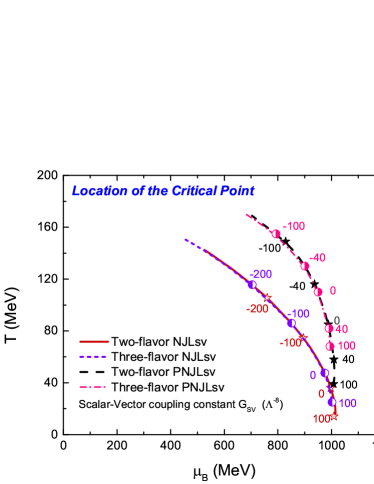
Figure 3: (Color online) Location of the critical point in two-flavor and three-flavor NJL models and PNJL models with the scalar-vector coupled interaction in the plane of temperature $T$ versus baryon chemical potential $\mu_{B}$. The lines are obtained by changing the value of the coupling constant $G_{SV}$ with other parameters in the two-flavor and three-flavor (P)NJL models given in Table 1 and Table 2, respectively.

II.2 The three-flavor NJL model

Table 2: Parameters in the three-flavor NJL model Buballa (2005a); Ratti et al. (2006); Roessner et al. (2007).

$\Lambda$ [MeV]   $G_{S}\Lambda^{2}$	$K\Lambda^{5}$	$m_{u,d}$ [MeV]	$m_{s}$ [MeV]
631.4   1.835	9.29	5.5	135.7
$M_{u,d}$ [MeV]	$M_{s}$ [MeV]	$\langle\bar{u}u\rangle^{1/3}$ [MeV]	$\langle\bar{s}s\rangle^{1/3}$ [MeV]
335	527	-246.9	-267

The three-flavor NJL model includes also the strange quark, which plays an important role in the partonic dynamic of heavy-ion collisions at high collision energies, The Lagrangian density in this model is given by Buballa (2005a)

$$\mathcal{L}_{\text{NJL}}^{\text{SU(3)}} = \mathcal{L}_{0}+\mathcal{L}_{\text{S}}+\mathcal{L}_{\text{SV}}+\mathcal{L}_{\text{det}},$$ (12)

with

$$\mathcal{L}_{0} = \bar{\psi}(i\gamma^{\mu}\partial_{\mu}-\hat{m})\psi,$$

$$\mathcal{L}_{\text{S}} = G_{S}\sum_{a=0}^{8}[(\bar{\psi}\lambda^{a}\psi)^{2}+(\bar{\psi}i\gamma_{5}\lambda^{a}\psi)^{2}],$$

$$\mathcal{L}_{\text{det}} = -K[\text{det}\bar{\psi}(1+\gamma_{5})\psi+\text{det}\bar{\psi}(1-\gamma_{5})\psi],$$ (13)

where $\psi=(u,d,s)^{T}$ now represents the 3-flavor quark fields and $\hat{m}=\text{diag}(m_{u},m_{d},m_{s})$ is the corresponding current quark mass matrix. In the above, $\lambda^{a}$($a$=1,…,8) with $\lambda^{0}$ being the identity matrix multiplied by $\sqrt{2/3}$ are the Gell-Mann matrices. The Lagrangian density $\mathcal{L}_{\text{det}}$ is the Kobayashi-Maskawa-t’Hooft (KMT) interaction ’t Hooft (1976) that breaks $U(1)_{A}$ symmetry with ‘det’ denoting the determinant in comthe flavor space Buballa (2005b), i.e., $\text{det}(\bar{\psi}\Gamma\psi)=\sum_{i,j,k}(\bar{u}\Gamma q_{i})(\bar{d}\Gamma q_{j})(\bar{s}\Gamma q_{k})$. This term gives rise to six-point interactions in three flavors and is responsible for the flavor mixing effect. We assume in the present study that only $u$ and $d$ quarks can have the scalar-vector coupled interaction, so the term $\mathcal{L}_{\text{SV}}$ has the same form as in Eq. (2).

In the mean-field approximation Vogl and Weise (1991b), the gap equations in the three-flavor NJL model for the quark in-medium effective masses including that ($M_{s}$) of the strange quark are given by

$$M_{u} = m_{u}-4G_{S}\phi_{u}+2K\phi_{d}\phi_{s}$$

$$-2G_{SV}(\rho_{u}+\rho_{d})^{2}(\phi_{u}+\phi_{d}),$$

$$M_{d} = m_{d}-4G_{S}\phi_{d}+2K\phi_{u}\phi_{s}$$

$$-2G_{SV}(\rho_{u}+\rho_{d})^{2}(\phi_{u}+\phi_{d}),$$

$$M_{s} = m_{s}-4G_{S}\phi_{s}+2K\phi_{u}\phi_{d}.$$ (14)

Besides the light quark condensates $\phi_{u}$ and $\phi_{d}$ as in the two-flavor NJL model, there is also the strange quark condensate given by

$$\phi_{s}=2N_{c}\int\frac{d^{3}p}{(2\pi)^{3}}\frac{M_{s}}{E_{s}}(n^{+}_{s}+n^{-}_{s}-1),$$ (15)

where $n^{\pm}_{s}=[e^{\beta(E_{s}\mp\mu_{s})}+1]^{-1}$ with $E_{s}=(M_{s}^{2}+{\bf p}^{2})^{1/2}$ and $\mu_{s}$ being the the strange quark chemical potential. The thermodynamic potential of the system can then be written as

$$\Omega_{\text{NJL}}^{\text{SU(3)}} = 2G_{S}(\phi^{2}_{u}+\phi^{2}_{d}+\phi^{2}_{s})$$ (16)

$$+ 3G_{SV}(\phi_{u}+\phi_{d})^{2}(\rho_{u}+\rho_{d})$$

$$- 4K\phi_{u}\phi_{d}\phi_{s}-2N_{c}\sum_{i=u,d,s}\int_{0}^{\Lambda}\frac{\text{d}^{3}p}{(2\pi)^{3}}E_{i}$$

$$- 2T\sum_{i=u,d,s}\int\frac{\text{d}^{3}p}{(2\pi)^{3}}(z^{+}(E_{i})+z^{-}(E_{i})).$$

To calculate the thermodynamic quantities of a quark matter in the three-flavor NJL model, we employ the parameters $m_{u}=m_{d}=5.5$ MeV, $m_{s}=135.7$ MeV, $G_{S}\Lambda^{2}=1.835$, $K\Lambda^{5}=9.29$, and a cut-off $\Lambda=631.4$ MeV Buballa (2005a), which are summarized in Table 2 together with the quark in-medium masses and condensates. The locations of the critical point in the temperature and baryon chemical obtained from the three-flavor NJL model with the scalar-vector coupled interaction are shown in Fig. 3 by the short dashed line. This line is almost identical to the solid line from the two-flavor NJL model except that the critical point in the three-flavor case moves to a higher temperature and smaller baryon chemical potential compared to the two-flavor case when the same $G_{SV}$ is used in the two calculations. The main reason for this similarity is because the parameters in the two-flavor and three flavor NJL models (see Tables 1 and 2) give similar properties of the QCD vacuum, e.g., the quark condensates and effective masses in vacuum. Results from these two models will not be identical if one uses different values for the parameters Buballa (2005a).

In principle, one can also include the scalar-vector coupled interactions for strange quarks. In this case, the dependence of the critical temperature on the value of $G_{SV}$ becomes much weaker than the results shown in the above, and this is because the in-medium mass of strange quark is much larger than the light quark masses, which makes it much harder to reach the chiral limit like the light quarks. Since the purpose of present study is to obtain a flexible critical point in the QCD phase diagram by tuning the strength of the scalar-vector coupled interaction, we have thus neglected the scalar-vector coupled interaction of the strange quark in the three-flavor NJL and PNJL models.

II.3 The NJL model with Polyakov loop

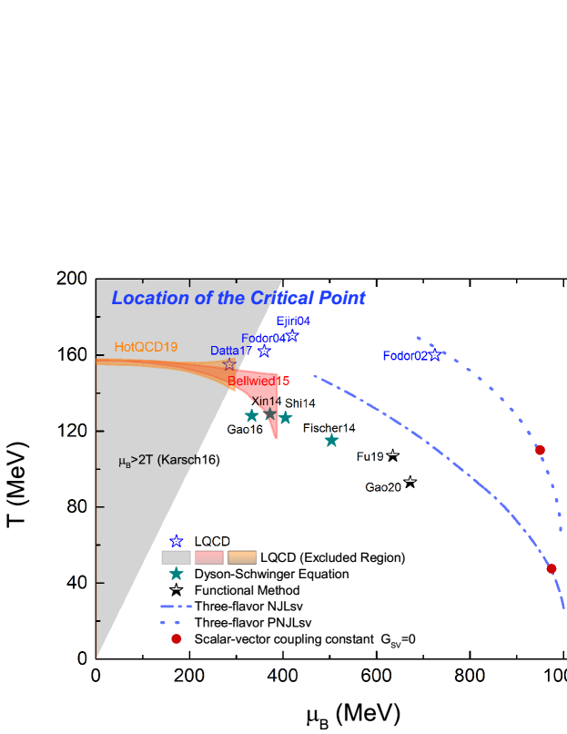
Figure 4: (Color online) Comparison of the location of the critical point in the plane of temperature $T$ versus baryon chemical potential $\mu_{B}$ from the three-flavor NJL (dash line) and PNJL (dotted line) models by varying the value of the scalar-vector coupling constant $G_{SV}$, with red solid circles denoting that obtained with $G_{SV}=0$, with predictions from LQCD Ejiri et al. (2004); Fodor and Katz (2004); Datta et al. (2013); Karsch et al. (2016); Datta et al. (2017); Bellwied et al. (2015); Bazavov et al. (2019), Dyson-Schwinger equation Xin et al. (2014); Fischer et al. (2014); Shi et al. (2014); Gao et al. (2016), and the functional renormalization method Fu et al. (2019); Gao and Pawlowski (2020).

To include also the confinement-deconfinement phase transition, a constant temporal background gauge field representing the Polyakov loops $\Phi$ and $\bar{\Phi}$ has been added to the NJL model Fukushima (2008). This so-called PNJL model changes the NJL Lagrangian density to

$$\mathcal{L}_{\text{PNJL}} = \bar{\psi}(i\gamma^{\mu}D_{\mu}-\hat{m})\psi+\mathcal{L}_{\text{S}}+\mathcal{L}_{\text{SV}}$$ (17)

$$- \mathcal{U}(\Phi[A],\bar{\Phi}[A],T),$$

where the covariant derivative is defined as $D^{\mu}=\partial^{\mu}-iA^{\mu}$ with $A^{\mu}=g\mathcal{A}^{\mu}_{a}(x)\lambda_{a}/2=\delta_{0}^{\mu}A_{0}$ being the $SU(3)$ gluon field in the Polyakov gauge and $g$ being the QCD strong coupling constant. The effective potential $\mathcal{U}$ for the Polyakov loops is given by

$$\frac{\mathcal{U}(\Phi,\bar{\Phi},T)}{T^{4}}=-\frac{1}{2}a(T)\bar{\Phi}\Phi+$$

$$b(T)\text{ln}[1-6\bar{\Phi}\Phi+4(\bar{\Phi}^{3}+\Phi^{3})-3(\bar{\Phi}\Phi)^{2}],$$ (18)

with

$$a(T)=a_{0}+a_{1}\left(\frac{T_{0}}{T}\right)+a_{2}\left(\frac{T_{0}}{T}\right)^{2},$$

$$b(T)=b_{3}\left(\frac{T_{0}}{T}\right)^{3},$$ (19)

where the parameters $a_{0}=3.51$, $a_{1}=-2.47$, $a_{2}=15.2$, and $b_{3}=-1.75$ are fitted to the results from the LQCD calculations of the thermodynamic properties of a pure gluon system Ratti et al. (2006); Roessner et al. (2007). For the temperature parameter $T_{0}$, its value is 270 MeV, corresponding to the critical temperature for the deconfinement phase transition of a pure gluon matter at zero baryon chemical potential Fukugita et al. (1990). The inclusion of quarks leads to a smaller value of $T_{0}=210$ MeV.

The grand potential of a quark matter at finite temperature and quark baryon potential in the PNJL model has a similar expression to Eq. (6) for the two-flavor or Eq. (16) for the three-flavor NJL model except the expression in Eq. (7) is replaced by

$$z_{\Phi}^{\pm}=\text{ln}[1+3(\bar{\Phi}+\Phi\text{e}^{-\beta(E_{i}\mp\mu_{i}^{*})})\text{e}^{-\beta(E_{i}\mp\mu_{i}^{*})}$$

$$\qquad+\text{e}^{-3\beta(E_{i}\mp\mu_{i}^{*})}].$$ (20)

As in the NJL model, the quark condensate and quark density are obtained by minimizing the grand potential, i.e., $\frac{\partial\Omega_{\text{PNJL}}^{\text{SU(3)}}}{\partial\phi_{i}}=\frac{\partial\Omega_{\text{PNJL}}^{\text{SU(3)}}}{\partial\rho_{i}}=0$. Their expressions are similar to those given in Eqs.(10) and (11) except the color-averaged equilibrium quark occupation numbers $n_{i}^{\pm}$ are replaced by

$$n_{\Phi}^{\pm} = \frac{\bar{\Phi}\text{e}^{2\beta(E\mp\mu^{*})}+2\Phi\text{e}^{\beta(E\mp\mu^{*})}+1}{e^{3\beta(E\mp\mu^{*})}+3\bar{\Phi}e^{2\beta(E\mp\mu^{*})}+3\Phi e^{\beta(E\mp\mu^{*})}+1}.$$

From the above expression, one can see that the quark distribution retains the normal Fermi-Dirac form at high temperature when the Polyakov loops are $\Phi=\bar{\Phi}=1$, while it becomes the Fermi-Dirac form with a reduced temperature $T/3$ at low temperature when $\Phi=\bar{\Phi}=0$. Hence, the critical temperature in the PNJL model is generally higher than that in the NJL model as the quarks in PNJL model experience a lower effective temperature. Note that the PNJL model at zero temperature is identical to the NJL model.

Minimizing the grand potential with respect to the Polyakov loops, i.e., $\frac{\partial\Omega_{\text{PNJL}}^{\text{SU(3)}}}{\partial\Phi}=\frac{\partial\Omega_{\text{PNJL}}^{\text{SU(3)}}}{\partial\bar{\Phi}}=0$, leads to the following mean-field equations for $\Phi$ and $\bar{\Phi}$:

$$\partial_{\Phi}\mathcal{U}$$

$$=6T\sum_{i=u,d,s}\int\frac{d^{3}p}{(2\pi)^{3}}\left[\frac{\text{e}^{-\beta(E_{i}-\mu_{i}^{*})}}{\exp(z_{\Phi}^{+}(E_{i}))}+\frac{\text{e}^{-2\beta(E_{i}+\mu_{i}^{*})}}{\exp(z_{\Phi}^{-}(E_{i}))}\right],$$

$$\partial_{\bar{\Phi}}\mathcal{U}$$

$$=6T\sum_{i=u,d,s}\int\frac{d^{3}p}{(2\pi)^{3}}\left[\frac{\text{e}^{-2\beta(E_{i}-\mu_{i}^{*})}}{\exp(z_{\Phi}^{+}(E_{i}))}+\frac{\text{e}^{-\beta(E_{i}+\mu_{i}^{*})}}{\exp(z_{\Phi}^{-}(E_{i}))}\right].$$

In Fig. 3, we show the locations of the critical point in the plane of temperature and baryon chemical potential obtained from both the two-flavor and the three-flavor PNJL model with the inclusion of the quark scalar-vector coupled interaction. As shown by the dashed line for the two flavor PNJL model and the dash-dotted line for the three-flavor NJL model, the effects of $G_{SV}$ are similar in these two cases. We also see that the effect of $G_{SV}$ on the critical chemical potential is smaller in the PNJL model than in the NJL model for both the two-flavor and the three-flavor case.

We further compare in Fig. 4 the critical point obtained from the three-flavor NJL (dash line) and PNJL (dotted line) models by varying the value of $G_{SV}$, with solid circles denoting those obtained with $G_{SV}=0$, with selected predictions from LQCD Ejiri et al. (2004); Fodor and Katz (2004); Datta et al. (2013); Karsch et al. (2016); Datta et al. (2017); Bellwied et al. (2015); Bazavov et al. (2019), Dyson-Schwinger equation Xin et al. (2014); Fischer et al. (2014); Shi et al. (2014); Gao et al. (2016), and the functional renormalization method Fu et al. (2019); Gao and Pawlowski (2020). Predictions from other effective methods can be found in Refs. Stephanov (2004) and references therein. It is seen that with sufficiently attractive scalar-vector coupled interaction, the locations of the critical point in the NJL and PNJL models can be brought closer to those predicted from these first principle approaches.

III conclusions

Based on the NJL model with both two flavors and three flavors as well as with the inclusion of Polyakov loops, we have studied the effect of the eight-fermion scalar-vector coupled interaction, which has no effects on the QCD vacuum properties, on the critical endpoint of the first-order QCD phase transition line in the QCD phase diagram. We have found that the location of the critical point in the temperature and baryon chemical potential plane is extremely sensitive to the strength of this interaction and can be easily shifted by changing its value. This flexible dependence of the quark equation of state due to the quark scalar-vector coupled interaction is very useful for locating the phase boundary in QCD phase diagram by comparing the experimental data with results from transport model simulations Li and Ko (2017) or hydrodynamic calculations based on equations of states from such generalized NJL and PNJL models.