Deep-Edge: An Efficient Framework for Deep Learning Model Update on Heterogeneous Edge

Abstract

Deep Learning (DL) model-based AI services are increasingly offered in a variety of predictive analytics services such as computer vision, natural language processing, speech recognition. However, the quality of the DL models can degrade over time due to changes in the input data distribution, thereby requiring periodic model updates. Although cloud data-centers can meet the computational requirements of the resource-intensive and time-consuming model update task, transferring data from the edge devices to the cloud incurs a significant cost in terms of network bandwidth and are prone to data privacy issues. With the advent of GPU-enabled edge devices, the DL model update can be performed at the edge in a distributed manner using multiple connected edge devices. However, efficiently utilizing the edge resources for the model update is a hard problem due to the heterogeneity among the edge devices and the resource interference caused by the co-location of the DL model update task with latency-critical tasks running in the background. To overcome these challenges, we present Deep-Edge, a load- and interference-aware, fault-tolerant resource management framework for performing model update at the edge that uses distributed training. This paper makes the following contributions. First, it provides a unified framework for monitoring, profiling, and deploying the DL model update tasks on heterogeneous edge devices. Second, it presents a scheduler that reduces the total re-training time by appropriately selecting the edge devices and distributing data among them such that no latency-critical applications experience deadline violations. Finally, we present empirical results to validate the efficacy of the framework using a real-world DL model update case-study based on the Caltech dataset and an edge AI cluster testbed.

I Introduction

The past decade has seen substantial progress in Deep Learning (DL), particularly Deep Neural Networks (DNNs), leading to its widespread adoption in various domains, such as medicine [1], geology [2] and vehicular navigation [3]. DL models are trained using a large amount of data and have outperformed previous AI-based approaches. However, training a DL model is a resource-intensive and time-consuming task. Various distributed DL frameworks, such as Tensorflow [4], MXNET [5] and Ray [6], have been developed to reduce the training time by distributing the training workload among multiple machines (cluster) consisting of one or more Graphics Processing Units (GPUs) or Application Specific Integrated Circuits (ASICs), such as Tensor Processing Units (TPUs).

However, an application composed of a deep learning component can experience degradation in accuracy over time due to changes in the input data distribution. This phenomenon is referred to as Concept Drift. To overcome model staleness and incorporate changes due to input data streams, continual learning [7] has been used to periodically refine the static models by re-training the existing model using recent data. Figure 1 shows the lifecycle of a machine learning model in production, where an inference API hosts the DL model. Recent data, along with the predicted and actual labels are stored in a data store that is fed to the model update process based on a user-defined trigger to replace the stale model with an updated one.

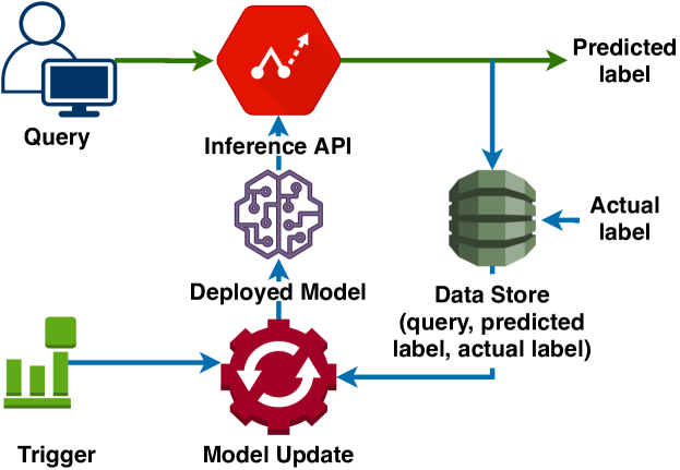
Figure 1: Machine learning model life cycle

I-A Emerging Trends

Traditionally, the model update occurs in the cloud, where the data collected from the edge of the network is transferred to the cloud data centers. However, the availability of powerful and reliable GPU-accelerated edge AI products, such as NVIDIA’s Jetson family (TX2, Nano, Xavier) and Google’s edge TPU [8] (Coral), has made continual learning viable using edge devices. In particular, the edge devices are suitable for performing the model update due to the following reasons:

• The computational power of edge devices is sufficient for updating small to medium-sized DNNs (up to 150 million parameters), such as VGG, Resnet, Inception, Mobilenet.

• The duration of the model update task is far less than the initial model training time, as fewer full data iterations (epochs) are required.

• Performing model update at the edge avoids costly data transfers to the cloud.

• Using edge devices for the model update also handles data privacy concerns and reduces data security threats.

I-B Challenges

There exist several resource managers (e.g., Borg [9], Tetricsched [10], Barista [11]) for different kinds of workloads in the cloud environment that perform static and dynamic scheduling. However, most of the approaches do not apply to edge clusters, which illustrate higher levels of heterogeneity among the edge devices. The heterogeneity can be the result of different physical characteristics of the devices, such as the number of processors, CUDA cores, memory, etc. or due to the workload associated with the devices. Another challenge is caused by the performance interference resulting from resource contention due to tasks running in the background. Running the resource-intensive model update task can cause the background latency-critical tasks to miss deadlines leading to Service-Level Objective (SLO) violations [12]. Hence, the selection of an edge device to participate in the model update task should be contingent on the latency constraints of the background tasks. Resolving these challenges calls for a custom resource manager for DL model update workloads at the edge by considering the timing constraints of the background applications, the computational capabilities, and workloads of the individual edge devices along with the structure and characteristics of the DL jobs.

I-C Overview of Technical Contributions

In this paper, we propose Deep-Edge, a custom resource management framework for DL model update jobs to minimize the model update time by distributing the re-training workloads among a set of heterogeneous edge devices while adhering to the timing and latency constraints of the background tasks. We focus on data-parallel distributed training based on the centralized parameter server architecture. Specifically, we make the following contributions:

• We define unified monitoring, profiling, and deployment framework for model update tasks at the edge.

• We build accurate performance and interference models for DL model update task and latency-critical background tasks by profiling them under various system metrics, such as CPU, GPU, Memory utilization, etc.

• We formulate an optimization problem that incorporates the edge node selection and workload distribution decisions to minimize the overall model update time.

• We present a polynomial-time heuristic solution based on the timing constraints, the performance, and interference models of the model update and background tasks.

• We show the efficacy of the framework by evaluating the accuracy of the proposed solution on a real-world DL model update task based on the Caltech dataset and an edge AI cluster testbed.

I-D Paper Organization

The rest of the paper is organized as follows: Section II provides a brief introduction to DL and the challenges associated with updating a DL model using edge devices. Section III describes the problem formulation. Section IV discusses the design and implementation of the Deep-Edge framework. Section V evaluates Deep-Edge using a prototypical case study. Section VI presents a survey of existing solutions in the literature and compares them with Deep-Edge. Finally, Section VII presents the concluding remarks and future directions.

II Background and Motivation

Deep learning is the process of learning very complex functions by multiple transformations of the raw input to an abstract high-level representation [13]. Training a DL model such as a DNN is an iterative process that requires a large amount of data due to the number of parameters to be learned. The data is typically divided into shards, which are further sliced up into batches. The processing of a batch constitutes a training step, which involves: 1) inferring the output and calculating a loss function for each data sample in the batch (forward pass); 2) determining the gradients based on the loss function, i.e., changes to be made to the parameters of the DL model (backward pass); and 3) updating the parameters of the DL model for the given batch of samples. When all batches are processed, one epoch is said to be completed.

Training a DL model is a resource-intensive and time-consuming task. Several machine learning frameworks, such as MXNET, TensorFlow, and Ray, support distributed training in which the task is divided among multiple workers. Primarily, there are two kinds of parallelism associated with distributed training: 1) Model Parallelism has all workers learn a part of the DL model parameters while working on the complete dataset; 2) Data Parallelism involves sharding the dataset among different workers such that each worker learns the complete DL model parameters while working on the part of the dataset. In this work, we focus on data-parallelism-based distributed training.

There exists another classification in distributed training based on how the knowledge (parameters) learned by individual workers is shared across the group. Most DL frameworks implement either centralized or decentralized architecture for storing and sharing the updated parameters of a DL model. In the centralized architecture, all workers compute forward and backward passes locally and send the gradients to a central entity, called the parameter server, for updating the parameters based on an optimization algorithm such as Stochastic Gradient Descent (SGD). The parameters are then pulled back by the workers to continue the next training step. In the decentralized architecture, no central entity exists, and the workers exchange among each other the locally learned gradients. The decentralized architecture is not suitable for the model update at the edge because it incurs higher transfer costs due to the need to broadcast the learned gradients to all the other workers.

There are also two kinds of training loops associated with data-parallel, centralized distributed training: 1) Synchronous training loop, where each worker waits for the others to finish a training step before starting another step, i.e., the training progress is synchronized at each step; 2) Asynchronous training loop, where the training progress is not synchronized, and the parameter server updates the model parameters upon receiving the gradients from each worker. Using an asynchronous training loop is more favorable for the model update at the edge as it avoids the costly synchronization overhead. Figure 2 shows a centralized parameter server-based distributed training with $n$ asynchronous training loops.

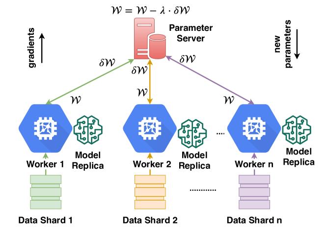
Figure 2: Parameter server architecture for distributed DL training

The following subsections motivate the development of Deep-Edge by describing the impact of heterogeneity and resource interference on the model update task and latency-critical tasks running in the background.

II-A Impact of Heterogeneity on Model Update Time

Typically, an equal amount of data is distributed among the workers in multi-machine training. However, this approach can result in a longer time to complete because of the heterogeneity of the edge devices. For instance, we observed that TX2 is 30% faster on an average in completing a training step than Nano when updating a state-of-the-art Inception model [14] using the Caltech-256 Object category dataset [15]. Figure 3 shows the cumulative distribution of time to complete one step, where the average step times for TX2 and Nano are 1.89 and 2.69 seconds, respectively. Thus, equal distribution can lead to underutilization of edge resources. Moreover, the performance of the model update task can be impacted by the state of the node (e.g., CPU, GPU, Memory utilization) as shown in Figure 4, where an initial GPU utilization of 88% and 66% for the two devices increases the average step time by almost 20%. Hence, an intelligent data sharding policy is required by considering the actual states of the workers.

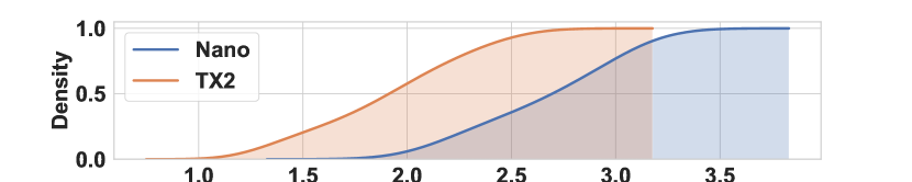
Figure 3: Variation of step time w.r.t device type

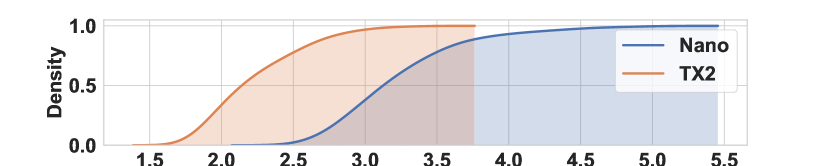
Figure 4: Increase in step time due to resource contention

II-B Impact of Resource Interference on Background Tasks

The selection of a worker to participate in the model update task depends upon the degree of interference that can be tolerated by the worker’s background tasks. Each curve in Figure 5 shows the sensitivity of a resource (GPU, CPU, Memory) towards the DL model update task. The x-axis represents the initial resource utilization before running the DL update task, and the y-axis represents the final resource utilization. The updated system state (defined in terms of the system metrics) can lead to deadline violation of a latency-critical background task. Moreover, adding more workers can reduce the training throughput, as described in [16]. Hence, a resource scheduler for a DL task needs to find the optimal number of workers, along with the ideal data shards, without violating the SLO constraints of background tasks.

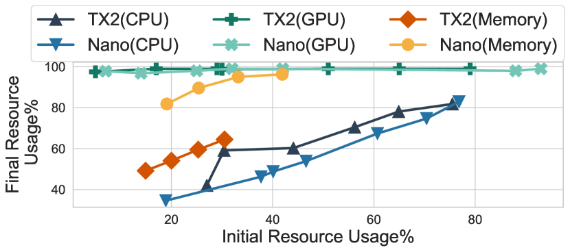
Figure 5: Initial and final resource usage along multiple resource dimensions.

III Problem Formulation

In this paper, we consider distributed data-parallel training of DL models using a centralized parameter server architecture with asynchronous training loops. This section models the various costs involved in the DL model update process formulates an optimization problem to minimize the overall cost and states our assumptions.

III-A Cost Models

We consider a set $\mathcal{W}=\{w_{1},w_{2},\dots,w_{N}\}$ of $N$ heterogeneous edge nodes (or workers) that can perform distributed training, and a set $\mathcal{M}$ of data samples for training a DL model. Let $\mathcal{D}=\{d_{1},d_{2},\dots,d_{N}\}$ denote the size of data shards among all the workers, i.e., the number of data samples assigned to each worker, such that $\sum_{i=1}^{N}d_{i}=|\mathcal{M}|$.

III-A1 Data transfer cost

All data samples are assumed to be initially stored in a data store $ds\in\mathcal{DS}$, where $\mathcal{DS}$ is the set of data stores. The data samples need to be transferred to each edge worker for training. Let $transfer^{ds}_{i}$ denote the cost of transferring a single data sample from data store $ds$ to edge node $w_{i}$. Thus, the total transfer cost for node $w_{i}$ is given by $Transfer^{ds}_{i}=d_{i}\cdot transfer^{ds}_{i}$.

III-A2 Initialization cost

After receiving the data samples, each edge node $w_{i}$ incurs a one-time initialization cost, denoted by $Initialize_{i}$, before the training begins. This cost is DL framework-dependent and consists mainly of data pre-processing (un-packing), loading the DL model, setting up the logical DL cluster, etc.

III-A3 Training cost

The data shards at each worker $w_{i}$ are further divided into batches of size $b_{i}$, and let $\mathcal{B}=\{b_{1},b_{2},\dots,b_{N}\}$ denote the set of batch sizes for all workers. The cost to process each batch includes the time to do forward propagation (for computing the loss function) and the time to do backward propagation (for computing the gradients). Let $forward_{i}$ denote the forward propagation time for one data sample on worker $w_{i}$, and let $backward_{i}$ denote the backward propagation time, which is typically incurred once per batch and is not related to the size of the batch. Given a batch size $b_{i}$, the per-sample compute time on worker $w_{i}$ is then given by $t_{i}^{compute}=forward_{i}+backward_{i}/b_{i}$.

After processing each batch, each worker $w_{i}$ pushes the gradients to a centralized parameter server $ps$ for update, and then pulls the updated parameters before continuing to train on the next batch. Let $push^{ps}_{i}$, $update^{ps}$ and $pull^{ps}_{i}$ denote the time to push, update and pull the parameters, respectively. Then, the update time is given by the sum of these three times, i.e., $t_{i}^{update}=push^{ps}_{i}+update^{ps}+pull^{ps}_{i}$. Since each worker $w_{i}$ has $B_{i}\approx d_{i}/b_{i}$ batches, the total time to process all the data samples on the worker, called an epoch, is given by:

$$epochTime_{i} =B_{i}\Big{(}b_{i}\cdot t_{i}^{compute}+t_{i}^{update}\Big{)}.$$

Note that the per-sample compute time $t_{i}^{compute}$ to perform forward and backward propagation depends on the computing capability of the individual worker as well as the background tasks running on the worker. Further, the update time $t_{i}^{update}$ to perform push, update, and pull on each worker is also not fixed. It depends on the batch size, the total number of deployed workers, as well as the states of the workers and the parameter server.

III-A4 Total cost

The total cost includes the data transfer and initialization costs for all workers, followed by the asynchronous training and update costs from different workers. Note that all costs are expressed in terms of time.

As the set of workers is assumed to be heterogeneous, some of them may not be deployed for training (e.g., due to high data transfer cost or low computational capability). Typically, having more workers will reduce the workload of each participating worker, thus decreasing the compute time (i.e., $t_{i}^{compute}$). However, it may also incur a larger update time (i.e., $t_{i}^{update}$) due to contentions caused by different workers trying to update the parameters at the same time.

Let $\gamma_{i}\in\{0,1\}$ denote a binary variable indicating if worker $w_{i}$ will be deployed for training or not, i.e., $\gamma_{i}=1$ if $d_{i}>0$ and $\gamma_{i}=0$ if $d_{i}=0$. Then, for all workers to complete a specified number of epoches, denoted by $numEpoch$, the total cost of distributed training can be expressed as:

$$Tota\_cost =\max_{i}\{\gamma_{i}\cdot\big{(}Transfer^{s}_{i}+Initialize_{i}$$

$$~{}~{}~{}~{}~{}~{}~{}+epochTime_{i}\cdot numEpoch\big{)}\}$$

III-B Optimization Problem

The goal of Deep-Edge is to minimize the overall cost of distributed training on a set of heterogeneous edge nodes by choosing a data sharding scheme $\mathcal{D}$, the batch sizes $\mathcal{B}$, as well as the number of deployed workers while subject to some system and performance constraints. The following states the optimization problem:

minimize $$Total\_cost$$

subject to $$b_{\min}\leq b_{i}\leq b_{\max},~{}\forall i$$ (1)

$$0\leq d_{i}\leq|\mathcal{M}|,~{}\forall i$$ (2)

$$\sum\nolimits_{i}d_{i}=|\mathcal{M}|$$ (3)

$$pressure_{i}^{a}\leq\delta^{a},~{}\forall a\in backApp_{i},\forall i$$ (4)

Constraint (1) requires the batch size to be within the range of minimum and maximum system-specific batch size, which could be determined by the DL model or the device’s memory constraint. Constraints (2) and (3) require that each worker receives a portion of the data samples, and altogether they cover the entire set of data samples. Finally, Constraint (4) requires that, for each worker $w_{i}$, the pressure to its set of background applications, $backApp_{i}$, due to running the distributed training job on the same device, should be contained to be within an application-specific threshold $\delta_{a}$ for each application $a\in backApp_{i}$ in order not to violate the SLO of the application. The estimation of the pressure function to a background task, and the sensitivity function for the training job will be discussed further in Section IV.

As the objective function (i.e., $Total\_cost$) and the pressure constraint in the above optimization problem have complex, non-linear relationships with the decision variables (i.e., $\mathcal{D},\mathcal{B}$), they cannot be expressed analytically. Thus the problem cannot be solved using standard solvers and/or analytical techniques. Therefore, we will design efficient heuristic solutions for the problem, which will be described in Section IV.

III-C Assumptions

We assume that the user specifies the maximum number of epochs (i.e., $numEpoch$) required for the training of the DL model, which is independent of the configuration of the workers. The user also provides the model trigger condition, and the model is only updated whenever the trigger condition is received. As the DL model is usually updated on a large amount of data, we further assume that the one-time transfer cost (i.e., $Transfer^{s}_{i}$) and initialization cost (i.e., $Initialize_{i}$) are negligible compared to the total training cost. Finally, we assume that the location of the parameter server is given, and we do not need to select a node as a parameter server based on some specific criteria.

IV Design and Implementation of Deep-Edge

This section presents the design and implementation details of Deep-Edge by describing the architecture model, various components of the framework, and its modes of operation.

IV-A Architecture Model

The architecture model is shown in Figure 6 consists of $K$ edge nodes, out of which $N$ are workers, $O$ are data stores, and $P$ are parameter servers, and they are represented by the disjoint sets $\mathcal{W}$, $\mathcal{DS}$ and $\mathcal{PS}$, respectively. These edge nodes form a local area network and are connected via a layer 2 switch. As mentioned in the previous section, the nodes in $\mathcal{W}\cup\mathcal{PS}$ form the DL model update cluster, where the worker nodes perform the actual re-training and the parameter server nodes act as a central repository for model parameters. The nodes in $\mathcal{DS}$ store data samples for the model update task.

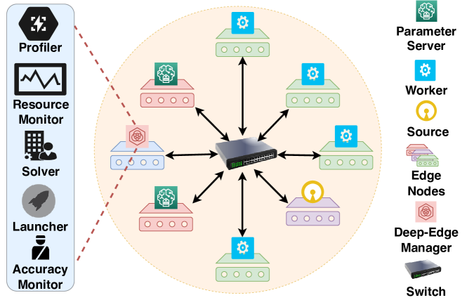
Figure 6: Deep-Edge architecture

One of the nodes in $\mathcal{DS}$ also acts as a Deep-Edge Manager (DEM), which implements the Deep-Edge framework. DEM consists of a collection of components that enables profiling, resource scheduling and runtime monitoring of the DL cluster. The components are hosted as REST endpoints as http://<ip>:<port>/<endpt_name>?<endpt_args>, where ip is the IP address of the host, port is the port associated with the DEM, and endpt_name, endpt_args are the name and input arguments of the endpoint. The following subsections describe the different components and modes of operation associated with the DEM.

IV-B Components of Deep-Edge Manager

The DEM consists of five components, which together provide a unified solution for profiling, scheduling, and monitoring the DL model update tasks.

IV-B1 Profiler

Deep-Edge uses a data-driven approach to estimate various performance and interference models (i.e., $t^{compute}$, $t^{update}$ and $pressure$ experienced by the background applications). This component allows both latency-critical and model update tasks to be profiled against stress points along the dimensions of CPU, GPU, and Memory utilization. The Profiler accepts different system metrics and stress points as the input arguments. Deep-Edge uses CPU, Memory, Disk I/O stressors from the well-known library Stress-ng [17], and the GPU load stressing application is based on the NVIDIA Cuda-10 library.

IV-B2 Solver

This component implements the scheduling strategy to identify the candidate workers and their respective data shards. The Solver takes the number of data samples, the current state of the edge cluster along with the performance and interference models as inputs, and outputs a data sharding scheme. The scheduling strategy is explained in more detail in Section IV-C2

IV-B3 Resource Monitor

The Resource Monitor maintains a map of active workers in the edge cluster and periodically monitors the ongoing model update tasks. This component is responsible for re-triggering the model update task in response to worker node failure.

IV-B4 Launcher

This component is responsible for launching applications (DL & stressing) on the worker and parameter server nodes. It accepts three different kinds of arguments: a) Stressor arguments; b) DL arguments; and c) Logging arguments. The Stressor arguments include parameters for the different stressing applications. The DL arguments include machine learning specific arguments, such as batch size, number of epochs, optimizer, etc. The Logging arguments include the file path for creating log files.

IV-B5 Accuracy Monitor

Deep-Edge allows dynamic stopping of the model update task by tracking the accuracy of the validation set. The update task is launched based on the initial estimate of the number of epochs provided by the user, and the estimate of the number of epochs is refined in an online fashion using logistic regression, similar to Optimus [16].

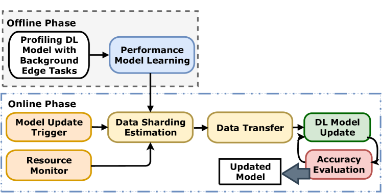
Figure 7: Modes of operation

IV-C Modes of Operation

The operation of DEM can be categorized into two modes, offline and online, as illustrated in Figure 7. In the offline or design mode, we build machine learning models to predict the execution times of the DL re-training task and latency-critical background tasks. In the online mode, appropriate workers, along with batch size distribution and data shards, are calculated based on the developed performance models such that re-training time is minimized while adhering to the SLO constraints imposed by the background applications. The online mode also handles worker failures by trying to restart the DL re-training task. The details of these features are described in the following.

IV-C1 Performance and Interference Modeling

Deep-Edge uses a data-driven approach for modeling the performance of DL re-training tasks on each node as well as the interference experienced by latency-critical background tasks. The performance of the DL re-training task is measured by the time to complete one epoch, $epochTime_{i}$, which is the function of per-sample compute time, $t^{compute}_{i}$, and update time, $t^{update}_{i}$, as defined in the optimization problem. Here, $t^{compute}_{i}$ depends upon the node type, state and batch size. We describe node state as a vector of system metrics containing CPU, GPU and Memory utilizations. However, $t^{update}_{i}$ depends not only on the node state but also on the complete batch distribution, state of the parameter server and number of workers. We define two functions, EstComputeTime and EstUpdateTime, to model the relation between the state of the DL cluster and $t^{compute}_{i}$ and $t^{update}_{i}$ as shown in Equations (5) and (6) below, where $\mathcal{X}_{i}$ and $b_{i}$ represent the state and batch size associated with worker $w_{i}\in\mathcal{W}$, $\mathcal{B}$ is the batch size distribution and $\mathcal{X}_{ps}$ is the state of the parameter server.

$$t^{compute}_{i}=\texttt{EstComputeTime}(\mathcal{X}_{i},b_{i})$$ (5)

$$t^{update}_{i}=\texttt{EstUpdateTime}(\mathcal{X}_{i},\mathcal{B},\mathcal{X}_{ps},|\mathcal{W}|)$$ (6)

In order to create an interference profile of the DL re-training task, we model interference as performance degradation experienced by the background applications. We use a two-step approach to quantify performance degradation, i.e., increase in execution time. In the first step, we model the effects of running the DL re-training task on a node whose state is described in Equation (7). The function, EstState, gives the relation between the initial state of the node, $\mathcal{X}^{initial}_{i}$, and its new state, $\mathcal{X}^{new}_{i}$, while executing the DL re-training task. Since the system metrics can vary during the execution of the re-training task, we use the 95th percentile value statistic. The second step involves learning the performance degradation, i.e., the pressure on a background task, as a function of the new node state, defined by EstExecTime as shown in Equation (8).

$$\mathcal{X}^{new}_{i}=\texttt{EstState}(\mathcal{X}^{initial}_{i})$$ (7)

$$pressure^{a}_{i}=\texttt{EstExecTime}(\mathcal{X}^{new}_{i})$$ (8)

The models mentioned above are learned by first performing a sensitivity analysis to understand the importance/influence of the prospective features. Based on the candidate feature set obtained after the sensitivity analysis, regression models are learned. In Deep-Edge, we use H2O’s AutoML framework [18] to find the best hyper-parameter tuned algorithm.

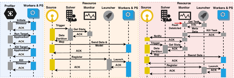
Figure 8: Event sequence diagram: Profiling (Left), Job scheduling (Middle), Failure handling (Right)

IV-C2 Resource Scheduling

Figure 8 (Middle) shows the sequence of events pertaining to a new request of model update. A data store makes a request to DEM’s solver endpoint to trigger the mode update. Upon the receipt of the request, the Solver gets the updated states of the workers, i.e., the number of prospective workers and their respective states (system metrics). Then, the Solver calculates the candidate worker nodes, data shards, and batch distribution using the scheduling strategy illustrated in Algorithm 1. The data and batch distributions are sent back to the data store to initiate data and base model transfer. After successful transmission, the data store registers the task information, such as the number of workers, data source, worker hostnames, data shards, and batch distribution, with the Launcher. In the end, the Launcher sends the acknowledgment back to the data store after successfully starting the DL re-training task on the selected workers.

The heuristic presented in Algorithm 1 provides an efficient solution to the optimization problem described in Section III. The input of the algorithm includes the workers’ state map $\mathcal{X}=[\mathcal{X}_{1},\mathcal{X}_{2},\dots,\mathcal{X}_{N}]$, where $\mathcal{X}_{i}$ = [$\mathcal{X}_{i}^{cpu}$, $\mathcal{X}_{i}^{gpu}$, $\mathcal{X}_{i}^{mem}$] represents the state of worker $w_{i}\in\mathcal{W}$, the parameter server’s state $\mathcal{X}_{ps}$ = [$\mathcal{X}_{ps}^{cpu}$, $\mathcal{X}_{ps}^{gpu}$, $\mathcal{X}_{ps}^{mem}$], the number of data samples $\mathcal{M}$, the stopping threshold $\varepsilon$, and the maximum number of iterations $\tau$ attempted by the algorithm. The output of the algorithm is the data distribution $\widetilde{\mathcal{D}}$ and the batch size distribution $\widetilde{\mathcal{B}}$, such that $d_{i}\in\widetilde{\mathcal{D}}$ and $b_{i}\in\widetilde{\mathcal{B}}$ indicate, respectively, the data shard and batch size associated with worker $w_{i}\in\mathcal{W}$. Note that if any worker $w_{k}\in\mathcal{W}$ is not selected for the model update task, the algorithm will return $d_{k}=0$ and $b_{k}=0$ for that worker.

The heuristic computes the data shards and batch distribution in an iterative fashion, where the initial estimate of the size of all data shards is set to be $\infty$ [Lines 2-3]. Using the initial data shards and the memory utilization of a node, the corresponding batch size $b_{i}$ is calculated [Line 6] using the function GetMaxBatchSize, which provides the maximum batch size given the current memory utilization of the node while enforcing adherence of the memory constraint described in the optimization problem. With the batch size estimates, $t^{compute}_{i}$, $t^{update}_{i}$ and $t^{total}_{i}$ are calculated for all the workers [Lines 7-9]. A refined data shard $d_{i}$ for worker $w_{i}$ is then calculated based on $t^{total}_{i}$ to balance the workloads of all the workers [Line 10]. After calculating the refined data shards, all workers check for adherence for resource interference constraints [Lines 11-22]. A worker is removed from the DL cluster [Lines 19-21] if any of its background tasks will experience deadline violations [Lines 14-17]. The cycle [Lines 5-28] repeats until the data shards in two consecutive iterations are almost the same, i.e., the $\mathcal{L}^{2}$ norm is less than a threshold $\varepsilon$, or the maximum number of iterations $\tau$ have been reached [Lines 24-26].

Then, we calculate the epoch time based on the data shards, which is given by the maximum time taken by any worker to process the data samples assigned [Line 29]. Note that, based on our proportional data sharding scheme, the difference between the epoch times from the different workers should be minimal (only due to rounding-off errors). If the resulting epoch time is better than the best one we have found so far, we remember the configuration as a potential solution [Lines 30-32]. Finally, to explore if better solutions are possible, we calculate the effect of removing the slowest worker (in terms of the total per-sample training time) on the overall epoch time [Lines 33-34]. As fewer workers are now present, this may affect the update time for each remaining worker, which will, in turn, affect the data shards and the epoch time. This process is performed iteratively until removing a worker no longer improves the overall epoch time, in which case the algorithm will eventually terminate [Line 36]. The final data shard size will then be given by the best one found so far.

1

2Initialize: $min\_t^{*}\leftarrow\infty$, $\widetilde{\mathcal{W}}\leftarrow\phi$, $\widetilde{\mathcal{B}}\leftarrow\phi$, $\widetilde{\mathcal{D}}\leftarrow\phi$; $Iter$ $\leftarrow$ 0

3 $d_{i}=\infty,~{}\forall w_{i}\in\mathcal{W}$;

4 $\mathcal{D}\leftarrow\{d_{1},d_{2},\dots,d_{N}\},~{}Iter\leftarrow 0$;

5 while True do

6       while True do

7             $b_{i}\leftarrow\min(\textnormal{GetMaxBatchSize}(\mathcal{X}_{i}^{mem}),d_{i}),~{}\forall w_{i}\in\mathcal{W}$;

8             $t_{i}^{compute}\leftarrow\textnormal{EstComputeTime}(\mathcal{X}_{i},b_{i}),~{}\forall w_{i}\in\mathcal{W}$;

9             $t^{update}_{i}\leftarrow\textnormal{EstUpdateTime}(\mathcal{X}_{i},\mathcal{X}_{ps},\mathcal{B},|\mathcal{W}|),\forall w_{i}\in\mathcal{W}$;

10             $t^{total}_{i}\leftarrow t^{compute}_{i}+t^{update}_{i}/b_{i},\forall w_{i}\in\mathcal{W}$;

11             $d_{i}=\frac{|\mathcal{M}|}{t^{total}_{i}\cdot\sum_{w_{i}\in\mathcal{W}}\frac{1}{t^{total}_{i}}},\forall w_{i}\in\mathcal{W}$;

12             for each $w_{i}\in W$ do

13                   $flag\leftarrow$ False;

14                   for each a $\in$ backApp_i  do

15                         if pressure${}_{i}^{a}$ > $\delta_{i}^{a}$ then

16                               $flag\leftarrow$ True;

17                               break; $\triangleright$ Constraint violated

18                              

19                         end if

20                        

21                   end for

22                  if $flag$ then

23                         $\mathcal{W}\leftarrow\mathcal{W}\setminus w_{i},b_{i}\leftarrow 0,d_{i}\leftarrow 0$; $\triangleright$ Remove worker

24                        

25                   end if

26                  

27             end for

28            $\mathcal{D}_{new}\leftarrow\{d_{1},d_{2},\dots,d_{N}\},~{}Iter$++;

29             if ($||\mathcal{D}_{new}$ - $\mathcal{D}||_{2}\leq\epsilon$) $\lor$ ($Iter==\tau$) then

30                   break;

31             end if

32            $\mathcal{D}\leftarrow\mathcal{D}_{new}$;

33            

34       end while

35      $epochTime=\max_{w_{i}\in\mathcal{W}}(d_{i}\cdot t^{total}_{i})$;

36       if $epochTime<min\_t^{*}$ then

37             $min\_t^{*}\leftarrow epochTime$;

38             $\widetilde{\mathcal{W}}\leftarrow\mathcal{W}$ , $\widetilde{\mathcal{B}}\leftarrow\mathcal{B}$ , $\widetilde{\mathcal{D}}\leftarrow\mathcal{D}$;

39             $w_{k}\leftarrow\operatorname*{arg\,max}_{w_{i}\in\mathcal{W}}(t^{total}_{i})$; $\triangleright$ Find slowest worker

40             $\mathcal{W}\leftarrow\mathcal{W}\setminus w_{k},b_{k}\leftarrow 0,d_{k}\leftarrow 0$; $\triangleright$ Remove worker

41            

42       else

43            break;

44       end if

45      

46 end while

Algorithm 1 Scheduling Heuristic

IV-C3 Fault Tolerance

When a worker node experiences a failure while executing a model update task either due to process crash or node failure, the Resource Monitor in the DEM will detect such events and trigger the re-launching of the task. The DEM uses a three-strike rule, i.e., a worker will not be considered part of the DL cluster if it has experienced at least three interruptions while running a model update task. Figure 8 (Right) highlights the sequence of events as a result of worker failure. After detecting a worker failure, the Resource Monitor gets the DL task information such as data shards, batch distribution, worker hostnames, data source and task id from the Launcher, and kills the model update processes on the remaining workers. After the processes are killed, the Resource Monitor notifies the appropriate data source to re-trigger the model update task.

V Evaluation Results

In this section, we present the evaluation results of different phases of the Deep-Edge framework.

V-A Experimental Setup

Testbed: Our testbed comprises one NVIDIA Jetson TX2 (256-core NVIDIA Pascal GPU, 8GB memory, Dual-Core NVIDIA Denver 2 64-Bit CPU and Quad-Core ARM Cortex-A57), three NVIDIA Jetson Nano (128-core Maxwell GPU, Quad-Core ARM Cortex-A57, 4GB memory), and two Raspberry Pi 4 (Broadcom BCM2711, Quad-core Cortex-A72 (ARM v8), 4GB memory). These devices are connected by a layer 2 switch. One Raspberry Pi acts as a parameter server while the second acts as a data store and also hosts the DEM.

Workloads: The model update task consists of updating a base DNN, namely Inception [14], with 3,855 data samples from the Caltech-256 dataset [15] using MXNET [5]. The base Inception model is created using transfer learning [7], where the last layer of a pre-trained Inception model based on Imagenet [19] is replaced by a new layer. We trained the base model (last layer) with 2,700 data points to reach an accuracy of 60%. The latency-critical background task is based on a distributed real-time computer vision application, which performs image reconstruction from multiple video streams where an initial image processing step is done in parallel on multiple edge devices. The image processing step involves identifying scale and rotation invariant descriptors (features) using Scale Invariant Feature Transform (SIFT) [20]. The latency-critical task constitutes executing SIFT on the acquired frame and sending the serialized SIFT features along with the original frame to an image stitching server over a UDP socket every 200ms. The size and resolution of the acquired frame are 56KB and 640$\times$320, respectively.

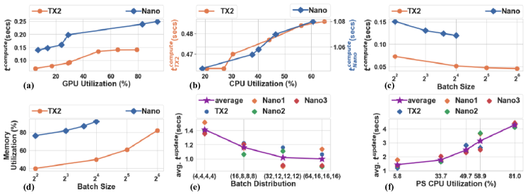
Figure 9: Sensitivity analysis

V-B Performance Modeling

We performed sensitivity analysis along the dimensions of GPU, CPU, and Memory utilization, as well as the number of workers and batch size. The following behaviors are observed:

• Increasing the GPU utilization increases the compute time $t^{compute}$ (Figure 9(a)).

• Increasing the CPU utilization increases the compute time $t^{compute}$ (Figure 9(b)).

• Increasing the batch size of the DL model update process decreases the compute time $t^{compute}$ (Figure 9(c)).

• Increasing the batch size of the DL model update process increases the memory utilization (Figure 9(d)).

• Increasing the batch size of the DL model update process decreases the update time $t^{update}$ (Figure 9(e)).

• Increasing the CPU utilization of the parameter server increases the update time $t^{update}$ (Figure 9(f)).

• Increasing the number of workers increases the DL model update time $t^{update}$.

• Increasing Memory utilization does not affect the throughput of the model update task. However, insufficient free memory can result in terminating a process by the OS.

Based on the above observations, we considered CPU utilization, GPU utilization, and batch size as the candidate features to learn the function EstComputeTime and added server CPU utilization, the number of workers along with batch distribution of all nodes to the above list as the set of features to learn the function EstUpdateTime. The function, EstState, has multiple outputs in nature, i.e., GPU, CPU, Memory, and a separate regressor is learned for each one of them. We extend the label with the feature name to indicate the individual regression model (for instance, EstState^mem represents the memory regressor). GetMaxBatchSize uses EstState^mem recursively to identify the maximum feasible batch size to run the model update task on a node. Finally, EstExecTime uses all system metrics of the node as features to predict the time to finish the latency-critical task. We used H2O’s AutoML framework [18] to select the best regression algorithm as well as to perform hyperparameter tuning. Table I highlights the number of data points, regression algorithm along with the accuracy for all learned functions. In particular, the gradient boosting based ensemble methods outperformed other algorithms with an average MAPE (mean absolute percentage error) of 3.433% overall for all the learned functions.

Device	Function	Data-points	Accuracy
		(train/test)	(MAPE)
Nano	EstComputeTime	1386/264	1.668 $\pm$ 2.074
Nano	EstUpdateTime	1386/264	9.617 $\pm$ 7.383
Nano	EstStategpu	1386/264	1.498 $\pm$ 3.9
Nano	EstStatecpu	1386/264	5.21 $\pm$ 4.53
Nano	EstStatemem	1386/264	1.508 $\pm$ 1.306
Nano	EstExecTime	1386/264	1.73 $\pm$ 0.21
TX2	EstComputeTime	378/72	5.916 $\pm$ 6.721
TX2	EstUpdateTime	378/72	7.721 $\pm$ 6.598
TX2	EstStategpu	378/72	0.509 $\pm$ 0.479
TX2	EstStatecpu	378/72	6.294 $\pm$ 5.468
TX2	EstStatemem	378/72	0.894 $\pm$ 0.704
TX2	EstExecTime	378/72	1.48 $\pm$ 0.12
Pi	EstStatecpu	630/120	2.32 $\pm$ 1.58
Pi	EstStatemem	630/120	1.70 $\pm$ 1.15

TABLE I: Estimator results

V-C Scheduling

We compare the scheduling policy of Deep-Edge with the fairness-based scheduler adopted in many resource managers, such as Hadoop [21], Yarn [22] and Mesos [23]. We performed 120 random experiments, and in each experiment, all worker nodes are running the SIFT feature detector task along with some randomly selected stressors, such that the initial state of every node does not violate the deadline of the background application. Figure 10 highlights the average epoch times observed when using the Deep-Edge and the fairness schedulers. On average, the Deep-Edge scheduler reduced the epoch time by 1.54 times compared to the fairness scheduler without violating any deadline. Figure 11 shows a histogram of speedups for the DL task achieved by the Deep-Edge scheduler over the fairness scheduler. We can see that the speedup can be as high as 200%, and more than half of the experiments have a speedup of more than 50%.

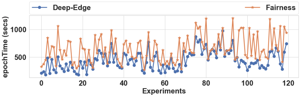
Figure 10: Epoch time distribution

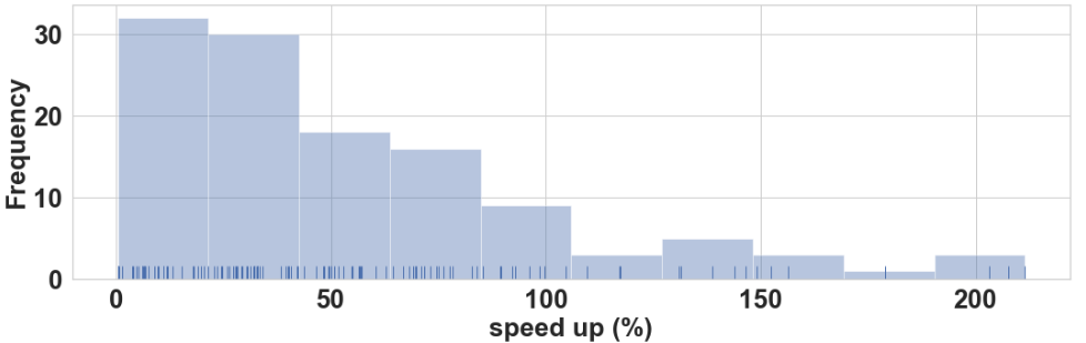
Figure 11: Speedup distribution

VI Related Work

This section provides a literature survey along the dimensions of interference aware resource management in edge devices and DL task scheduling.

VI-A Performance & Interference-aware Resource Management

Resource interference is studied extensively in the literature, and different approaches are proposed to understand and quantify interference. Paragon [24] presents an interference-aware job scheduler, in which an application’s performance is predicted using collaborative filtering. The performance prediction model is built by subjecting the target application by varying each resource stressor at a time. Authors in [25] studied the impact of co-located application performance for a single multi-core machine and developed a piece-wise regression model using cache contention and bandwidth consumption of co-located applications as input features. The ESP project [26] also uses a regression model to predict performance interference for every possible co-location combination. Pythia [27] proposed a linear regression model approach for predicting combined resource contention by training on a small fraction of the large configuration space of all possible co-locations. Both ESP and Pythia assume that they have a priori information of all possible running workloads, based on which an interference model is created for a new application. PARTIES [28] proposes a feedback-based controller to dynamically adjust resources between co-scheduled latency-critical applications using fine-grained monitoring and resource partitioning to guarantee the Quality-of-Service (QoS). INDICES [29] proposes interference aware fog server selection using a gradient boosting based performance model of latency-critical applications. The authors extend the same approach in [30] to offload a latency-critical task between fog and edge devices while considering user mobility. However, none of these approaches are designed for distributed tasks such as DL model re-training and do not consider GPU utilization.

VI-B Deep Learning Task Scheduling

There are several approaches in the scientific literature for resource allocation to achieve a variety of objectives in cloud settings such as Borg [9], Coral [31] and TetriSched [10], Morpheus [32]. However, the schedulers mentioned above are not designed for DL workloads. There are recent research efforts on GPU sharing for machine learning tasks. Baymax [33] explores GPU sharing as a way to mitigate both queuing delay and resource contention. Following that, Prophet [34] proposes an analytical model to predict the performance of GPU workloads. Gandiva [35] aims GPU time-sharing in shared GPU clusters through check-pointing at low GPU memory usage of the training job. CROSSBOW [36] proposes a dynamic task scheduler to automatically tune the number of workers to speed up the training and to use the infrastructure optimally. Optimus [16] also dynamically adjusts the number of workers and parameter servers to minimize the training completion time while achieving the best resource efficiency. SLAQ [37] targets the training quality of experimental ML models instead of models in production. It adopts an online fitting technique similar to Optimus to estimate the training loss of convex algorithms. Dorm [38] uses a utilization-fairness optimizer to schedule jobs. However, these approaches are not applicable for edge clusters as none of them considers resource interference while allocating heterogeneous resources for the DL model update task.

VII Conclusion and Future Work

This paper presents Deep-Edge, an interference aware DL model update framework for the edge devices that minimizes the re-training time by intelligently distributing data among edge nodes while adhering to the latency constraints of the background applications. We described different components of the framework and showed its efficacy by validating it against a realistic case study.

In the future, we would like to extend this work in three dimensions: 1) improving performance and interference models by adding more features such as memory and disk bandwidth; 2) adding support for Multi-Process Service (MPS) based GPU workloads; 3) including parameter server load balancing as part of the scheduling problem; and 4) considering a more diverse set of edge devices such as TPUs and FPGAs.

References

- [1] F. Milletari, N. Navab, and S.-A. Ahmadi, “V-net: Fully convolutional neural networks for volumetric medical image segmentation,” in 2016 Fourth International Conference on 3D Vision (3DV). IEEE, 2016, pp. 565–571.
- [2] L. Huang, X. Dong, and T. E. Clee, “A scalable deep learning platform for identifying geologic features from seismic attributes,” The Leading Edge, vol. 36, no. 3, pp. 249–256, 2017.
- [3] C. Chen, A. Seff, A. Kornhauser, and J. Xiao, “Deepdriving: Learning affordance for direct perception in autonomous driving,” in Proceedings of the IEEE International Conference on Computer Vision, 2015, pp. 2722–2730.
- [4] M. Abadi, P. Barham, J. Chen, Z. Chen, A. Davis, J. Dean, M. Devin, S. Ghemawat, G. Irving, M. Isard et al., “Tensorflow: A system for large-scale machine learning,” in 12th USENIX Symposium on Operating Systems Design and Implementation (OSDI 16), 2016, pp. 265–283.
- [5] T. Chen, M. Li, Y. Li, M. Lin, N. Wang, M. Wang, T. Xiao, B. Xu, C. Zhang, and Z. Zhang, “Mxnet: A flexible and efficient machine learning library for heterogeneous distributed systems,” arXiv preprint arXiv:1512.01274, 2015.
- [6] P. Moritz, R. Nishihara, S. Wang, A. Tumanov, R. Liaw, E. Liang, M. Elibol, Z. Yang, W. Paul, M. I. Jordan et al., “Ray: A distributed framework for emerging AI applications,” in 13th USENIX Symposium on Operating Systems Design and Implementation (OSDI 18), 2018, pp. 561–577.
- [7] H. Tian, M. Yu, and W. Wang, “Continuum: A platform for cost-aware, low-latency continual learning,” in Proceedings of the ACM Symposium on Cloud Computing, 2018, pp. 26–40.
- [8] M. Hosseinabady, M. A. B. Zainol, and J. Nunez-Yanez, “Heterogeneous fpga+ gpu embedded systems: Challenges and opportunities,” arXiv preprint arXiv:1901.06331, 2019.
- [9] A. Verma, L. Pedrosa, M. Korupolu, D. Oppenheimer, E. Tune, and J. Wilkes, “Large-scale cluster management at google with borg,” in Proceedings of the Tenth European Conference on Computer Systems, 2015, pp. 1–17.
- [10] A. Tumanov, T. Zhu, J. W. Park, M. A. Kozuch, M. Harchol-Balter, and G. R. Ganger, “Tetrisched: global rescheduling with adaptive plan-ahead in dynamic heterogeneous clusters,” in Proceedings of the Eleventh European Conference on Computer Systems, 2016, pp. 1–16.
- [11] A. Bhattacharjee, A. D. Chhokra, Z. Kang, H. Sun, A. Gokhale, and G. Karsai, “Barista: Efficient and scalable serverless serving system for deep learning prediction services,” in 2019 IEEE International Conference on Cloud Engineering (IC2E). IEEE, 2019, pp. 23–33.
- [12] A. Bhattacharjee, Y. Barve, S. Khare, S. Bao, Z. Kang, A. Gokhale, and T. Damiano, “Stratum: A bigdata-as-a-service for lifecycle management of iot analytics applications,” in 2019 IEEE International Conference on Big Data (Big Data). IEEE, 2019, pp. 1607–1612.
- [13] Y. LeCun, Y. Bengio, and G. Hinton, “Deep learning,” nature, vol. 521, no. 7553, pp. 436–444, 2015.
- [14] C. Szegedy, V. Vanhoucke, S. Ioffe, J. Shlens, and Z. Wojna, “Rethinking the inception architecture for computer vision,” in Proceedings of the IEEE conference on computer vision and pattern recognition, 2016, pp. 2818–2826.
- [15] G. Griffin, A. Holub, and P. Perona, “Caltech-256 object category dataset,” 2007.
- [16] Y. Peng, Y. Bao, Y. Chen, C. Wu, and C. Guo, “Optimus: an efficient dynamic resource scheduler for deep learning clusters,” in Proceedings of the Thirteenth EuroSys Conference, 2018, pp. 1–14.
- [17] C. I. King, “Stress-ng,” URL: http://kernel. ubuntu. com/git/cking/stressng. git/(visited on 28/03/2018), 2017.
- [18] [Online]. Available: https://www.h2o.ai/
- [19] O. Russakovsky, J. Deng, H. Su, J. Krause, S. Satheesh, S. Ma, Z. Huang, A. Karpathy, A. Khosla, M. Bernstein et al., “Imagenet large scale visual recognition challenge,” International journal of computer vision, vol. 115, no. 3, pp. 211–252, 2015.
- [20] D. G. Lowe, “Distinctive image features from scale-invariant keypoints,” International journal of computer vision, vol. 60, no. 2, pp. 91–110, 2004.
- [21] R. C. Taylor, “An overview of the hadoop/mapreduce/hbase framework and its current applications in bioinformatics,” in BMC bioinformatics, vol. 11, no. S12. Springer, 2010, p. S1.
- [22] V. K. Vavilapalli, A. C. Murthy, C. Douglas, S. Agarwal, M. Konar, R. Evans, T. Graves, J. Lowe, H. Shah, S. Seth et al., “Apache hadoop yarn: Yet another resource negotiator,” in Proceedings of the 4th annual Symposium on Cloud Computing, 2013, pp. 1–16.
- [23] B. Hindman, A. Konwinski, M. Zaharia, A. Ghodsi, A. D. Joseph, R. H. Katz, S. Shenker, and I. Stoica, “Mesos: A platform for fine-grained resource sharing in the data center.” in NSDI, vol. 11, no. 2011, 2011, pp. 22–22.
- [24] C. Delimitrou and C. Kozyrakis, “Paragon: Qos-aware scheduling for heterogeneous datacenters,” ACM SIGPLAN Notices, vol. 48, no. 4, pp. 77–88, 2013.
- [25] J. Zhao, X. Feng, H. Cui, Y. Yan, J. Xue, and W. Yang, “An empirical model for predicting cross-core performance interference on multicore processors,” in Proceedings of the 22nd international conference on Parallel architectures and compilation techniques. IEEE, 2013, pp. 201–212.
- [26] N. Mishra, J. D. Lafferty, and H. Hoffmann, “Esp: A machine learning approach to predicting application interference,” in 2017 IEEE International Conference on Autonomic Computing (ICAC). IEEE, 2017, pp. 125–134.
- [27] R. Xu, S. Mitra, J. Rahman, P. Bai, B. Zhou, G. Bronevetsky, and S. Bagchi, “Pythia: Improving datacenter utilization via precise contention prediction for multiple co-located workloads,” in Proceedings of the 19th International Middleware Conference, 2018, pp. 146–160.
- [28] S. Chen, C. Delimitrou, and J. F. Martínez, “Parties: Qos-aware resource partitioning for multiple interactive services,” in Proceedings of the Twenty-Fourth International Conference on Architectural Support for Programming Languages and Operating Systems, 2019, pp. 107–120.
- [29] S. Shekhar, A. D. Chhokra, A. Bhattacharjee, G. Aupy, and A. Gokhale, “Indices: exploiting edge resources for performance-aware cloud-hosted services,” in 2017 IEEE 1st International Conference on Fog and Edge Computing (ICFEC). IEEE, 2017, pp. 75–80.
- [30] S. Shckhar, A. Chhokra, H. Sun, A. Gokhale, A. Dubey, and X. Koutsoukos, “Urmila: A performance and mobility-aware fog/edge resource management middleware,” in 2019 IEEE 22nd International Symposium on Real-Time Distributed Computing (ISORC). IEEE, 2019, pp. 118–125.
- [31] V. Jalaparti, P. Bodik, I. Menache, S. Rao, K. Makarychev, and M. Caesar, “Network-aware scheduling for data-parallel jobs: Plan when you can,” ACM SIGCOMM Computer Communication Review, vol. 45, no. 4, pp. 407–420, 2015.
- [32] S. A. Jyothi, C. Curino, I. Menache, S. M. Narayanamurthy, A. Tumanov, J. Yaniv, R. Mavlyutov, Í. Goiri, S. Krishnan, J. Kulkarni et al., “Morpheus: Towards automated slos for enterprise clusters,” in 12th USENIX Symposium on Operating Systems Design and Implementation (OSDI 16), 2016, pp. 117–134.
- [33] Q. Chen, H. Yang, J. Mars, and L. Tang, “Baymax: Qos awareness and increased utilization for non-preemptive accelerators in warehouse scale computers,” ACM SIGPLAN Notices, vol. 51, no. 4, pp. 681–696, 2016.
- [34] Q. Chen, H. Yang, M. Guo, R. S. Kannan, J. Mars, and L. Tang, “Prophet: Precise qos prediction on non-preemptive accelerators to improve utilization in warehouse-scale computers,” in Proceedings of the Twenty-Second International Conference on Architectural Support for Programming Languages and Operating Systems, 2017, pp. 17–32.
- [35] W. Xiao, R. Bhardwaj, R. Ramjee, M. Sivathanu, N. Kwatra, Z. Han, P. Patel, X. Peng, H. Zhao, Q. Zhang et al., “Gandiva: Introspective cluster scheduling for deep learning,” in 13th USENIX Symposium on Operating Systems Design and Implementation (OSDI 18), 2018, pp. 595–610.
- [36] A. Koliousis, P. Watcharapichat, M. Weidlich, L. Mai, P. Costa, and P. Pietzuch, “Crossbow: scaling deep learning with small batch sizes on multi-gpu servers,” Proceedings of the VLDB Endowment, vol. 12, no. 11, pp. 1399–1412, 2019.
- [37] H. Zhang, L. Stafman, A. Or, and M. J. Freedman, “Slaq: quality-driven scheduling for distributed machine learning,” in Proceedings of the 2017 Symposium on Cloud Computing, 2017, pp. 390–404.
- [38] P. Sun, Y. Wen, N. B. D. Ta, and S. Yan, “Towards distributed machine learning in shared clusters: A dynamically-partitioned approach,” in 2017 IEEE International Conference on Smart Computing (SMARTCOMP). IEEE, 2017, pp. 1–6.