Complaint-driven Training Data Debugging
for Query 2.0

Abstract.

As the need for machine learning (ML) increases rapidly across all industry sectors, there is a significant interest among commercial database providers to support “Query 2.0”, which integrates model inference into SQL queries. Debugging Query 2.0 is very challenging since an unexpected query result may be caused by the bugs in training data (e.g., wrong labels, corrupted features). In response, we propose Rain, a complaint-driven training data debugging system. Rain allows users to specify complaints over the query’s intermediate or final output, and aims to return a minimum set of training examples so that if they were removed, the complaints would be resolved. To the best of our knowledge, we are the first to study this problem. A naive solution requires retraining an exponential number of ML models. We propose two novel heuristic approaches based on influence functions which both require linear retraining steps. We provide an in-depth analytical and empirical analysis of the two approaches and conduct extensive experiments to evaluate their effectiveness using four real-world datasets. Results show that Rain achieves the highest recall@k among all the baselines while still returns results interactively.

1. Introduction

Database researchers have long advocated the value of integrating model inference within the DBMS: data used for model inference is already in the DBMS, it brings the code (models) to the data, and it provides a familiar relational user interface. Early libraries such as MADLib (Hellerstein et al., 2012) provide this functionality by leveraging user-defined functions and type extensions in the DBMS. The recent and tremendous success of ML in recommendation, ranking, predictions, and structured extraction over the past decade have led commercial data management systems (SQLFlow, 2019; Agrawal et al., 2019; Hellerstein et al., 2012; LLC, 2019) to increasingly providing first-class support for in-DBMS inference: Google’s BigQuery ML (LLC, 2019) integrates native TensorFlow support, and SQLServer supports ONNX (Exchange, 2019) models. These developments point towards mainstream adoption of this new querying paradigm that we call Query 2.0.

Many companies already leverage Query 2.0 in their core business. CompanyX customers can define user cohorts using traditional and model-based predicates (details in Section 2). For example, Figure 1 finds and counts the number of active users in the previous month (active_last_month) that are likely to churn ($M_{\boldsymbol{\theta}}$.predict()). The latter predicate uses the model $M_{\boldsymbol{\theta}}$ to estimate whether the user will churn. Cohorts are used for email campaigns, downstream analyses, and client monitoring. In fact, 100% of the company’s user segmentation logic are performed within the DBMS. Beyond CompanyX, both industry (Logicblox, 2019; SQLFlow, 2019) and research (Li et al., 2019a; Kraska et al., 2013; Boehm et al., 2016; Lu et al., 2018; Jankov et al., 2019) are advocating for Query 2.0.

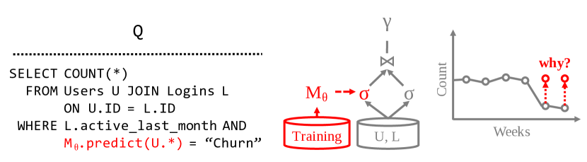
Figure 1. CompanyX cohort query, its workflow, and output visualization where the user specifies surprising output values. Training and model inference steps in red.

Unfortunately, Query 2.0 is considerably more challenging to debug than traditional relational queries because the results depend on not only the queried data  (e.g., U,L), but also the training data that are used to fit the predictive models used in the query. Training data are a major factor in determining a model’s accuracy, and when a model makes incorrect predictions, it is challenging to even identify the erroneous training records (Varma et al., 2018). Thus, even if the query and queried data are correct, errors in the training data can cause incorrect query results.

As one example, CompanyX tracks users on e-commerce websites and scrapes the pages for data to estimate user retention. They regularly retrain their model $M_{\boldsymbol{\theta}}$. However, systematic errors, such as changing the name of a product category or adding a new check-out step, can cause $M_{\boldsymbol{\theta}}$ to suddenly underestimate user churn likelihoods. Customers will see a surprising cohort size drop in the monitoring chart (Figure 1) and complain. Despite assertions and error checking in their workflow systems, CompanyX engineers still spend considerable time to find the training errors. Ideally, a debugging system can help them quickly identify examples of the training records that were responsible for the customer complaint.

Query debugging is not new, and there are existing explanation and debugging approaches for relational queries or machine learning models. SQL explanation (Wu and Madden, 2013; Meliou and Suciu, 2012; Roy et al., 2015; Abuzaid et al., 2018) uses user complaints of query results to identify queried records or predicates, and can fix the complaint through intervention (deleting those records). However in the context of Query 2.0, these methods would only identify errors in the queried data (e.g., U,L in Figure 1), rather than in $M_{\boldsymbol{\theta}}$’s training data.

On the other hand, case-based ML explanation algorithms (Khanna et al., 2019; Zhang et al., 2018) use labeled mispredictions to identify training points that, if removed, would fix the mispredictions. This is akin to specifying complaints over the intermediate outputs of the query (specifically, the outputs of the $M_{\boldsymbol{\theta}}\texttt{.predict()}$ predicate). Unfortunately, finding and labeling the mispredictions can take considerable effort. Further, users such as CompanyX’s customers only see the final chart.

To this end, we present Rain, a system to facilitate complaint-driven data debugging for Query 2.0. Given that the query and the queried data are correct, Rain detects label errors in the training data. Users simply report errors in intermediate or final query results as complaints, which specify whether an output value should be higher, lower, or equal to an alternative value, or if an output tuple should not exist. Rain returns a subset of training records that, if the models are retrained without those records, would most likely address the complaints. This problem combines aspects of integer programming, bi-level optimization, and combinatorial search over all subsets of training records—each is challenging in isolation, and together poses novel challenges faced neither by SQL nor ML explanation approaches.

To address these challenges, this paper describes and evaluates two techniques that bring together SQL and ML explanation techniques. Both iteratively identify training records that, if removed, are most likely to fix user complaints. TwoStep uses a two-step approach: it models the output of model inference as a view, and uses an existing SQL explanation method to identify records in the view that are responsible for user complaints. Those records are marked as mispredictions and then used as input to a case-based ML explanation algorithm. This method works well when SQL explanation can correctly identify the model mispredictions (or the user directly labels them). However, it can work poorly when there are many satisfying solutions for the complaints in the SQL explanation step; we call this complaint ambiguity, and provide theoretical intuition and empirical evidence that it causes TwoStep to incorrectly identify erroneous training points.

To address these limitations, the Holistic approach models the entire pipeline—the query plan, model training, and user complaints—as a single optimization problem. This directly measures the effect of each training record on the user complaints, without needing to guess mispredictions correctly. We also provide theoretical intuition for when and why Holistic should be more effective than existing approaches that do not account for SQL queries nor user complaints. To summarize, our contributions include:

• A formalization of complaint-driven training data debugging for Query 2.0, along with motivating use cases.

• The design and implementation of Rain, a solution framework that integrates elements of existing SQL and case-based ML explanation algorithms. Rain supports SPJA queries that use differentiable models such as linear models and neural networks.

• TwoStep, which sequentially combines existing ILP-based SQL explanation approaches and ML influence analysis techniques. Our theoretical analysis shows that TwoStep is sensitive to the ILP’s solution space, and we empirically validate this in the experiments.

• Holistic, which combine user complaints, the query, and model training in a single problem that avoids the ambiguity issues in TwoStep.

• An extensive evaluation of Rain against existing explanation baselines. We use a range of datasets containing relational, textual, and image data. We validate our theoretical analyses: TwoStep is susceptible to performance degradation when ambiguity is high, and that approaches that do not use complaints are misled when there are considerable systematic training set errors. We find that Holistic’s accuracy dominates the other approaches—including settings where alternative approaches cannot find any erroneous training records—and iteratively returns training records in interactive time.

The remainder of this paper is organized as follows. Section 2 presents example use cases. Section 3 formally defines the Query 2.0 debugging problem and discusses the computational challenge. We propose two novel approaches to solve the problem. Section 4 presents their main ideas and Section 5 describes the overall system architecture and details. Experimental results are presented in Section 6, followed by related work (Section 7) and conclusion (Section 8).

2. Use case

Rain helps identify systematic errors in training datasets that cause model mispredictions that, later on, introduce errors in downstream analyses. These errors can come from errors in manual labeling, procedural labelling (Ratner et al., 2017), or automated data generation processes (Colyer, 2019). This section presents illustrative use cases that can benefit from complaint-based debugging.

2.1. Example Use Cases

E-commerce Marketing: CompanyX specializes in retail marketing. One of its core services manages email marketing campaigns for its customers. 10-20 ML models predict different user characteristics (e.g., will a user churn, product affinity). Customers see model predictions as attributes in views, and can use them, or raw user profile data, to create predicates to define user cohorts that are used in email campaigns and tracked over time (e.g., Figure 1).

For development simplicity, CompanyX uses Google BigQuery for model training, cohort creation, and monitoring; the queries are instrumented at different points to be visualized or monitored purposes. For example, customer-facing metrics dashboards visualize user cohort sizes over time, and customers can set alerts for when the cohort’s size drops or increases very rapidly, or exceeds some threshold.

CompanyX collects training data by scraping their customers’ e-commerce websites. However, changes to the website—such as adding a new check-out step, or changing a product category—can introduce systematic training errors that degrade the re-trained models, and ultimately trigger customer monitoring alerts and lead to customer questions. Pipeline monitoring is not enough to pinpoint the relevant training records, and their engineers are challenged to find and characterize the culprit training records.

Entity Resolution: A data scientist scrapes and trains a boolean classification model to use for entity resolution (e.g., given two business records, the model can determine whether they refer to the same real-world entity). However, when she uses it as the join condition over two business listings ($Listings_{1}\bowtie_{M_{\theta}.predict(*)=1}Listings_{2}$), she finds that the dining business categories have zero matches. She is sure that should not be the case and wants to understand why the classifier is incorrect.

Image Analysis: An engineer collects an image dataset and wants to train a hot-dog classifier. To create labels, she decides to use distant supervision (Zeng et al., 2015), and writes a programmatic labelling function. She uses the classifier to label a hot-dog, and a non-hot-dog dataset, equi-joins the two datasets on the predicted label, and plots the resulting count. She is surprised that there are many join results when there should not have been any, and complains that the count should be $0$.

2.2. Desired Criteria

Ultimately, manual pipeline and training data analysis is time-consuming and difficult. The above use cases highlight desired criteria that motivate complaint-driven data debugging for Query 2.0. First, is the ability to express data errors at different points in the query pipeline. This is important because users may only have access to specific output or intermediate results, or only have the time/expertise to comment on aggregated query results rather than manually label individual model predictions.

For example in Figure 1, the user may specify errors in the final query result, but an ML engineer may collect a sample of the model predictions in the output of $M_{\boldsymbol{\theta}}$.predict(U.*) and identify errors there as well. Similarly, another customer may find errors in a separate query that uses $M_{\boldsymbol{\theta}}$. The system should be able to use all pieces of information to identify the erroneous training records.

Second, users want to describe how data are incorrect and what their expectations of what correct data should look like. This requires a flexible complaint specification, rather than labeling mispredictions. For instance, when viewing Figure 1’s chart, the customer may state that the right-most erroneous points should be the value of the red points, or perhaps that they should not exist at all.

3. Problem Definition

This section formalizes the Query 2.0 debugging problem that we will study in this work. Also, we are going to discuss the computational hurdles in solving the problem efficiently.

3.1. Defining Query 2.0

Query 2.0 consists of a SQL query that embeds one or more ML models. This work focuses on Select-Project-Join-Aggregate (SPJA) SQL queries which have zero or more inner joins and embed a single classification ML model. In contrast to classification models, which assign probabilities to each class, regression does not always have probabilistic interpretations to the outputs. Supporting those models, the full SQL standard, and multiple models is left to future work. Note however, that the query can use the same model in multiple expressions.

Specifically, we support SP, SPJ, SPJA queries, such as:

⬇

SELECT agg($\cdot$), $\cdots$ FROM $R_{1},R_{2}\cdots R_{n}$

WHERE $C_{1}$ AND $\cdots$ AND $C_{m}$

GROUP BY $G_{1},G_{2}\cdots G_{k}$

where agg can be COUNT, SUM, or AVG, and each $C_{i}$ is either a filter condition or a join condition. Conjunctive and disjunctive predicates are supported as well. A model $M$ can appear in the SELECTION, WHERE, or GROUP BY clause (Table 1).

$Q_{1}:$	SELECT AVG(M.predict(R)) FROM R
$Q_{2}:$	SELECT COUNT(*) FROM R WHERE M.predict($R$)
$Q_{3}:$	SELECT * FROM $R_{1}$ and $R_{2}$ WHERE M.predict($R_{1}$) = M.predict($R_{2}$)
$Q_{4}:$	SELECT * FROM $R_{1}$ and $R_{2}$ WHERE M.predict($R_{1}$+$R_{2}$)
$Q_{5}:$	SELECT COUNT(*) FROM $R$ GROUP BY M.predict($R$)

Table 1. Query 2.0 examples. Model prediction can be embedded in an aggregation/projections ($Q_{1}$), filters ($Q_{2}$), join conditions ($Q_{3}$, $Q_{4}$), and group bys ($Q_{5}$).

• SELECTION: model prediction appears in an aggregation function, denoted by agg(M.predict). For example, if $M$ estimates customer salary, then $Q_{1}$ returns the average estimated salary.

• WHERE: model prediction appears in a filter condition or a join condition. For example, if $M$ predicts if a customer will churn or not, then $Q_{2}$ returns the number of customers that may churn. If $M$ extracts the user type, then $Q_{3}$ returns pairs of customers from two datasets that are the same user type (note that $Q_{3}$ is a SPJ query). Finally, if $M$ estimates if two records are the same entity, then $Q_{4}$ finds pairs of records that are the same entity.

• GROUP BY: model prediction appears in the GROUP BY clause. For example, if $M$ predicts the sentiment of a customer comment, then $Q_{5}$ returns the number of comments for each sentiment class (positive, neutral, or negative).

Let $T$ be the training set for model $M$ and $\mathcal{D}=\{R_{1},R_{2},\cdots,R_{n}\}$ denotes a database containing queried relations. The trained model $M$ will make predictions using data from $\mathcal{D}$. Given a query $Q$, we denote its output result over $\mathcal{D}$ by $Q(\mathcal{D};M(T))$. If the context is clear, the notation is simplified as $Q(\mathcal{D};T)$.

3.2. Complaint Models

A user may have a complaint about the query output $Q(\mathcal{D};T)$. We consider two types: value complaints and tuple complaints.

A value complaint lets the user ask why an output attribute value in $Q(\mathcal{D};T)$ is not equal to (larger than or smaller than) another value. In Figure 1, the user can specify why the two right-most low points in the visualization are not equal to (or larger than) the corresponding red points.

A tuple complaint lets the user ask why an output tuple in $Q(\mathcal{D};T)$ appears in the output. This can be because a tuple should have been filtered by a predicate that compares with a model prediction, or because an aggregated group exists when it should not. For example, the user may ask why a pair of loyal customers are in the join output of $Q_{3}$ in Table 1.

Definition 3.1 presents a formal definition of complaints.

Definition 3.1 (Complaint).

A complaint $c(t)$ is expressed as a boolean constraint over a tuple $t$ in the output relation $Q(\mathcal{D};T)$. The complaint can take two forms. The first is a Value Complaint over an attribute value $t[a]$, where $op\in\{=,\leq,\geq\}$ and $v$ may take any value in the attribute’s domain (if $t[a]$ is discrete, then $\leq,\geq$ do not apply):

(1) $$c_{\textsf{value}}\big{(}t,Q(\mathcal{D};T)\big{)}=\begin{cases}True,&\text{if}\ \textsf{ t[a] op v}\\ False,&\text{otherwise}\end{cases}$$

The second is a Tuple Complaint over the tuple $t$ which states that $t$ should not be in the output relation:

(2) $$c_{\textsf{tuple}}\big{(}t,Q(\mathcal{D};T)\big{)}=\begin{cases}True,&\text{if}\ \textsf{ $t\notin Q(\mathcal{D};T)$}\\ False,&\text{otherwise}\end{cases}$$

Multiple Complaints: The user may express multiple complaints against the result of $Q(\mathcal{D};T)$ or even against intermediate results of the query. In addition, if the user executed other queries using the same model $M(T)$, then complaints against those queries may also be used to identify training set errors. For ease of presentation, the text will focus on the single complaint case. However, the proposed approaches support multiple complaints, and we evaluate them in the experiments.

3.3. Problem Statement

Given a Query 2.0 query, there can be several ways to account for a user’s complaint $c$ by making changes to the training set $T$. For example, one might modify training examples in $T$, augment it with new training examples or even delete training examples. While all the above interventions make sense in different scenarios, for simplicity in this work we will focus on deletions of training examples from $T$. Given the definitions of the previous subsection, we are ready to define the Query 2.0 debugging problem.

Definition 3.2 (Query 2.0 Debugging Problem).

Given a training dataset $T$, a database $\mathcal{D}$ containing queried relations, a query $Q$, and a complaint $c$, the goal is to identify the minimum set of training records such that if they were deleted, the complaint would be resolved:

$$\underset{{\Delta\subseteq T}}{\text{minimize}} |\Delta|\hskip 28.45274pt$$

subject to $$c\big{(}t,Q(\mathcal{D};T\setminus\Delta)\big{)}=True$$

A brute force solution is to enumerate every possible set of deletions, and for each set, to retrain the model, update the query result, and evaluate the complaint. However, this needs to retrain up to $2^{|T|}$ models. The key is to reduce the number of models retrained. In the following, we propose two novel heuristic approaches which both reduce the number from exponential to linear.

4. Background and Preliminaries

In this section, we first introduce the concept of influence functions in ML explanation and then present the main ideas of our approaches.

4.1. Influence Functions

Influence functions provide a powerful way to estimate how the model parameters change by adding/deleting/updating a training point without retraining the model. For example, suppose one wants to know to delete which training point will lead to the best model parameters (i.e., the minimum model loss). A brute-force approach needs to enumerate every training point and retrain $|T|$ models. As will be shown below, influence functions do not involve any retraining.

Let a training set $T$ include $n$ pairs of feature vectors and labels $\boldsymbol{z}_{i}=(\boldsymbol{x}_{i},y_{i})$. An ML model parametrized by $\boldsymbol{\theta}$ is trained with the following loss function ($\ell$ is the training record loss):

$$L(\boldsymbol{\theta})=\frac{1}{n}\sum_{i=1}^{n}\ell(\boldsymbol{z}_{i},\boldsymbol{\theta})$$

A strongly convex function $L$ has a unique solution:

$$\boldsymbol{\theta}^{*}=\operatorname*{arg\,min}_{\boldsymbol{\theta}}L(\boldsymbol{\theta})$$

Adding a new training sample $\boldsymbol{z}$ with weight $\epsilon$ to the training loss leads to new set of optimal parameters $\boldsymbol{\theta}_{\epsilon}^{*}$:

(3) $$\boldsymbol{\theta}_{\epsilon}^{*}=\operatorname*{arg\,min}_{\boldsymbol{\theta}}\;\{L(\boldsymbol{\theta})+\epsilon\cdot\ell(\boldsymbol{z},\boldsymbol{\theta})\}$$

In general, we are interested in a closed-form expression of $\boldsymbol{\theta}_{\epsilon}^{*}$ for $\epsilon=\pm\frac{1}{n}$, which can estimate the effect of adding or removing a training point without retraining. Unfortunately, such a closed-form expression does not generally exist. The Influence Function approach quantifies the case when $\epsilon\approx 0$. By the first order optimality condition, since $\boldsymbol{\theta}_{\epsilon}^{*}$ minimizes the objective of Equation 3

$$\nabla_{\boldsymbol{\theta}}L(\boldsymbol{\theta}_{\epsilon}^{*})+\epsilon\cdot\nabla_{\boldsymbol{\theta}}\ell(\boldsymbol{z},\boldsymbol{\theta}_{\epsilon}^{*})=\boldsymbol{0}$$

The derivative of the equation above with respect to $\epsilon$, taking into account that $\boldsymbol{\theta}_{\epsilon}^{*}$ is a function of $\epsilon$, yields

$$\nabla_{\boldsymbol{\theta}}^{2}L(\boldsymbol{\theta}_{\epsilon}^{*})\frac{d\boldsymbol{\theta}_{\epsilon}^{*}}{d\epsilon}+\epsilon\cdot\nabla_{\boldsymbol{\theta}}^{2}\ell(\boldsymbol{z},\boldsymbol{\theta}_{\epsilon}^{*})\frac{d\boldsymbol{\theta}_{\epsilon}^{*}}{d\epsilon}+\nabla_{\boldsymbol{\theta}}\ell(\boldsymbol{z},\boldsymbol{\theta}_{\epsilon}^{*})=\boldsymbol{0}$$

Recent work has shown that using the derivative where $\epsilon=0$ is a good approximation of the change in model parameters for ($\boldsymbol{\theta}_{-1/n}^{*}$ or $\boldsymbol{\theta}_{1/n}^{*}$) (Giordano et al., 2019; Koh et al., 2019). Substituting $H_{\boldsymbol{\theta}^{*}}=\nabla^{2}_{\theta}L(\boldsymbol{\theta^{*}})$, where $H_{\boldsymbol{\theta}^{*}}$ is the Hessian of the loss function $L(\boldsymbol{\theta})$, and simple algebra derives the following when $\epsilon=0$:

$$\left.\frac{d\boldsymbol{\theta}_{\epsilon}^{*}}{d\epsilon}\right|_{\begin{subarray}{c}\epsilon=0\end{subarray}}=-H_{\boldsymbol{\theta}^{*}}^{-1}\nabla_{\boldsymbol{\theta}}\ell(\boldsymbol{z},\boldsymbol{\theta}^{*})$$

Note $\epsilon$ is dropped from $\boldsymbol{\theta}_{\epsilon}^{*}$ because it is set to $0$.

In our problem, we wish to approximate the effect of training points on user complaints. To do so, we will construct a differentiable function $q(\boldsymbol{\theta}_{\epsilon}^{*})$ that represents user complaints by encoding the SQL query, ML model, and user complaints. Section 5.3 and Section 5.2 describe two encoding procedures. Given $q(\boldsymbol{\theta}_{\epsilon}^{*})$, the effect of a training point is straightforward using the chain rule:

(4) $$\left.\frac{dq(\boldsymbol{\theta}_{\epsilon}^{*})}{d\epsilon}\right|_{\begin{subarray}{c}\epsilon=0\end{subarray}}=-\nabla_{\boldsymbol{\theta}}q(\boldsymbol{\theta}^{*})\ H_{\boldsymbol{\theta}^{*}}^{-1}\nabla_{\boldsymbol{\theta}}\ell(\boldsymbol{z},\boldsymbol{\theta}^{*})$$

Computing $H_{\boldsymbol{\theta}^{*}}^{-1}\nabla_{\boldsymbol{\theta}}\ell(\boldsymbol{z},\boldsymbol{\theta}^{*})$ can become a significant bottleneck as a naive implementation requires $\mathcal{O}(d^{2})$ space and $\mathcal{O}(d^{3})$ time. The authors of (Koh and Liang, 2017) leverage prior work (Martens, 2010) so that the total time and space complexity scales linearly in the dimension $d$. The calculation is posed as a linear system of equations, and approximately solved using the conjugate gradient algorithm. Instead of inverting the Hessian, the conjugate gradient relies on Hessian vector products that can be efficiently computed via backpropagation.

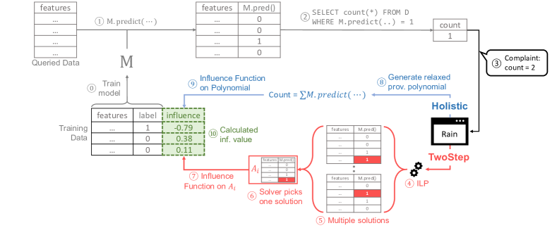
Figure 2. Rain architecture.

4.2. Main Ideas of Our Approaches

Unfortunately, influence functions cannot be directly applied to solve the Query 2.0 Debugging Problem since we need to calculate the impact of deletions of training points on a Query 2.0 query output, and SQL queries are not naturally differentiable.

We use two novel ideas to address this challenge. TwoStep first calculates the impact of deletions of training points on model parameters and then calculates the impact of the changes of model parameters on the query result. Holistic encodes a Query 2.0 query (both SQL and model parts) into a single differentiable function and then directly calculates the impact of deletions of training points on the query result.

We developed Rain, a Query 2.0 debugging system that implements TwoStep and Holistic approaches. The next section will describe the system details.

4.3. Why are Complaints Important?

Influence analysis can already be used to detect training errors based on the model loss without the need for complaints (Koh and Liang, 2017). The high sensitivity of the loss on a training record can be interpreted as a corrupted training record. Thus why are complaints important?

The main reason is that models can overfit to systematic training errors, and cause loss-based rankings to rank such errors arbitrarily low in terms of loss sensitivity. For example, changes in the checkout code might cause CompanyX to not log successful transactions for some customers; the trained model may then assume that similar customers will churn.

In contrast, SQL queries and complaints provide a vocabulary to specify systematic errors. This vocabulary generalizes existing work that labels individual mispredictions (Zhang et al., 2018; Khanna et al., 2019) or specifies undesirable prediction output distributions (Agarwal et al., 2018). Our experiments show that even a single aggregation complaint can identify systematic training errors more effectively than hundreds of labeled mispredictions.

5. The Rain System

This section describes the overall architecture of Rain, which uses either TwoStep (Section 5.2) or Holistic (Section 5.3) to solve the Query 2.0 Debugging Problem.

5.1. Architecture Overview

Rain (Figure 2) consists of a query processor that supports training machine learning models (step ), performing model inference (step ) and executing SQL queries based on the model outputs (step ). The user examines the output or intermediate result set of a query $Q$, and specifies a set of complaints $C$ (step complaints that the result should be 2 instead of 1). The optimizer uses a simple heuristic to choose between the two methods. As we will discuss in Section 5.2, TwoStep is preferable when there is a unique way to fix the querying set predictions that resolves $C$. For all other cases, Holistic is used.

TwoStep turns the complaints into a discrete ILP problem and uses an off-the-shelf solver (step ) to label a subset of the model inferences with their (estimated) correct predictions. If multiple satisfying solutions exist (step ), solvers will opaquely output one of the solutions dependent on the specific implementation (step ). The solution is encoded as an influence function to estimate how each training record “fixes” the mispredictions (step ). Holistic encodes the query and model training as a single relaxed provenance polynomial (step ) that serves as an influence function to estimate how much each training record “fixes” the complaints (step ). For both approaches, Rain finds the top $k$ training records by influence (step ).

Both approaches will first rerun $Q$ (step ) in a “debug mode” to generate fine-grained lineage metadata that encodes the optimization problem. Rain then runs a train-rank-fix scheme, where each iteration (re)trains the model (step ), reruns the query (step - ), finds and deletes the top training records by influence (step - ), and repeats. The result is a sequence of training records that comprise the output explanation $\Delta$. Assuming each iteration selects the top-$k$ training records, then Rain executes $\frac{|\Delta|}{k}$ iterations.

5.2. TwoStep Approach

Query 2.0 plans consist of relational pipelines and model inference. Since there are existing solutions to address each in isolation, the naive approach combines them into a TwoStep solution. This section describes this approach, and provides intuition on its strengths and limitations.

5.2.1. Approach Details

We now describe the SQL and Influence Analysis steps of TwoStep.

SQL Step: At a high level, TwoStep replaces each model inference expression, such as $M_{\theta}$.predict(U.*) in Figure 1, with a materialized prediction view containing the input’s primary key and the prediction result. Let $V_{M}$ be the prediction view for model $M$, and $D_{T}$ be the database containing the views. $Q(D;T)$ can be rewritten as $Q_{m}(D_{T})$ to instead refer to the model views rather than perform model inference directly. For instance, the query in Figure 1 would be rewritten as follows:

⬇

SELECT COUNT(*) FROM Users U, Logins L, $\mathbf{V_{m}}$

WHERE U.ID = L.ID AND U.ID = $V_{m}$.ID

AND L.active_last_month

AND $\mathbf{V_{m}}$.prediction = "Churn"

We build on Tiresias (Meliou and Suciu, 2012), which takes as input a set of complaints, along with attributes in queried relations that can be changed to fix those complaints. It translates the complaints and query into an ILP, where marked attributes are replaced with free variables that the solver (e.g., Gurobi (Gurobi Optimization, 2019), CPLEX (ILOG, 2014)) assigns. We mark the predicted attribute in the prediction views, and the objective minimizes the number of prediction changes.

The translation to an ILP relies on database provenance concepts. Each potential output of $Q_{m}$ defines a function over the prediction view that evaluates to $1$ if the tuple exists in the query output for the given prediction view or $0$ if not. In addition, each aggregation output value of $Q_{m}$ defines a function over the prediction view that returns the aggregation value. Prior provenance work (Green et al., 2007; Amsterdamer et al., 2011) shows how to translate the supported queries into symbolic representations of these functions also known as provenance polynomials, which Tiresias encodes as ILP constraints.

We illustrate the reduction for the example in Figure 1:

Example 5.1.

Let the query plan for Figure 1 first filter and join $L$ with $U$, and then apply the churn filter before the aggregation. Let $K$ be the number of the remaining rows after the join and filter on $L$, and $\boldsymbol{r}\in\{0,1\}^{K}$ be the binary model predictions over these rows. $r_{i}=1$ means the user is predicted to churn, and the query result is $\sum_{i=1}^{K}r_{i}$. If the user complains that the query output should be $X$, then the generated ILP is as follows, where $t_{i}\neq r_{i}$ means that record $i$ should be labeled as a misprediction:

(5) $$\underset{\boldsymbol{t}\in\{0,1\}^{K}}{\text{minimize}} \sum_{i=1}^{K}|t_{i}-r_{i}|\hskip 28.45274pt$$

subject to $$\sum_{i=1}^{K}t_{i}=X$$

Rain goes beyond this simple example and supports the queries and complaints described in Section 3.

Influence Analysis Step: The previous step assigns each record $\boldsymbol{x}_{i}$ a (possibly “corrected”) label $t_{i}$: $\{\boldsymbol{x}_{i},t_{i}\}_{i=1}^{K}$. Let $p_{t_{i}}(\boldsymbol{x}_{i},\boldsymbol{\theta})$ be the probability that model $M_{\boldsymbol{\theta}}$ predicts $\boldsymbol{x}_{i}$ to be class $t_{i}$, where $\boldsymbol{\theta}$ is the vector of the ML model parameters. We construct function $q(\boldsymbol{\theta})=-\sum_{i=1}^{K}p_{t_{i}}(\boldsymbol{x}_{i},\boldsymbol{\theta})$ that is used as input to an influence analysis framework (Koh and Liang, 2017; Hara et al., 2019; Zhang et al., 2018; Khanna et al., 2019). These frameworks return a ranking of training points that, if removed, are most likely to change the predictions of $\boldsymbol{x}_{i}$ to $t_{i}$; this indirectly addresses the user’s complaint.

For example, suppose we use the influence analysis framework of (Koh and Liang, 2017). TwoStep uses Equation 4 to score every training record. The initially trained model has optimal parameters $\boldsymbol{\theta}^{*}$. The training loss Hessian $H_{\boldsymbol{\theta}^{*}}$ and the training loss gradient of each training record $\nabla_{\boldsymbol{\theta}}\ell(\boldsymbol{z},\boldsymbol{\theta}^{*})$ are evaluated at $\boldsymbol{\theta}^{*}$. The function $q$ constructed by TwoStep is then substituted to encode the user’s complaint. Training records with large positive scores imply that their removal would decrease $q$ the most, implicitly addressing the complaint. TwoStep ranks these records at the top.

In most settings, the number of records not marked as a misprediction ($t_{i}=r_{i}$) is considerably larger than those marked as mispredictions ($t_{i}\neq r_{i}$), and encoding all of them slows down the influence analysis step. In our experiments, we only encode the marked mispredictions into $q(\cdot)$ in Equation 4, and empirically find that they result in comparable rankings as when encoding all records.

5.2.2. Limitations and Analysis

Although TwoStep is simple, there are several limitations due to the nature of the ILP formulation of the SQL step. First, the ILP problem can be ambiguous and is not guaranteed to identify the correct solution. Second, TwoStep depends on the user submitting a correct complaint. We discuss both limitations in this subsection.

Ambiguity: The generated ILP may not always have a unique solution. For example, Figure 2 shows how the ILP of a complaint on a COUNT aggregation can have multiple solutions $A_{1},A_{2},\dots,A_{n}$ (step ). We call such complaints ambiguous. Picking a solution $A_{i}$ in step that makes incorrect prediction fixes can negatively affect the influence step . Intuitively, a complaint with more ILP solutions should lead to worse rankings because, among all solutions that minimize the ILP problem, only a few minimize Definition 3.2. We identify two sources of ambiguity.

The first are aggregations. In Figure 2, flipping any single prediction $0$ is a valid and minimal solution, but only one solution is correct. The same argument extends to all the aggregates supported by Rain as all of them are symmetric with respect to their inputs.

The second are join and selection predicates. Consider a join $A\bowtie_{A.a=B.b}B$, where $A.a$ and $B.b$ are both estimated by a model $M$. If the user specifies that a join result should not exist, then one has to choose between changing $A.a$ or $B.b$. More generally, selection predicates that involve two or more model predictions can also be ambiguous.

Our appendix lists specific settings where ambiguity provably causes TwoStep to rank the true training errors arbitrarily low, thus forbidding us sampling multiple solutions from ILP to avoid bad results for the whole problem. Unfortunately, formally quantifying its effect in the general case is challenging because partially correct solutions $A_{i}$ can still yield high quality rankings depending on the model and the corrupted training records.

Our experiments vary the level of ambiguity and empirically suggest that TwoStep performs better when the number of solutions of the SQL step is smaller.

Complaint Sensitivity: The second limitation is due to the discrete formulation of the ILP: identifying correct assignments depends on the correctness of the complaint. For example, if the user selected a slightly incorrect $X$ in Equation 5, the satisfying assignments can be considerably different than the true mispredictions. Unfortunately, if the user finds surprising points in a visualization, she may have an intuition that the point should be higher or lower, but is unlikely to know its exact correct value. We see this sensitivity in our experiments.

5.3. Holistic Approach

In this section, we present the Holistic approach that addresses many of the limitations of TwoStep. The key insight is to connect training records with the user complaints by modeling the query probabilistically and interpreting the confidence of model predictions as probabilities. This lets us leverage prior work in probabilistic databases (Dalvi and Suciu, 2004; Kanagal et al., 2011) to represent Query 2.0 statements as a differentiable function that is amendable to influence analysis. Note that although provenance and influence analysis alone build on prior work, integrating them for the purpose of complaint-driven training data debugging is the key novelty.

5.3.1. Relaxation Approach

As noted above, the symbolic SQL query representations are not naturally differentiable due to discrete inputs (values in the prediction views), and thus are incompatible with an influence analysis framework. In contrast to TwoStep, Holistic leverages techniques from probabilistic databases (Kanagal et al., 2011; Dalvi and Suciu, 2004) to relax these functions of discrete inputs into continuous variable functions.

Revisiting Equation 5, Holistic substitutes the count of churn predictions with the expectation of the count. For example, let $r_{i}(\boldsymbol{\theta})$ be the boolean churn prediction and $p_{i}(\boldsymbol{\theta})$ be the churn probability assigned by $M_{\boldsymbol{\theta}}$, Holistic substitutes:

$$\sum_{i=1}^{K}r_{i}(\boldsymbol{\theta})\rightarrow\sum_{i=1}^{K}p_{i}(\boldsymbol{\theta}).$$

Unfortunately, expectations of provenance polynomials are not always straightforward to compute. Even calculating the expectation of a k-DNF formula is #P-complete (Kanagal et al., 2011). To sidestep the computational difficulty of exact probabilistic relaxation, we propose a tractable alternative under the simplifying assumption that variables and sub-expressions are independent. We first replace discrete predictions in the provenance polynomial with their corresponding probabilities (similar to $r_{i}(\boldsymbol{\theta})\rightarrow p_{i}(\boldsymbol{\theta})$ above). We then replace boolean operators (AND, OR, NOT) with continuous alternatives

$$x y \rightarrow x\cdot y$$ AND

$$x y \rightarrow 1-(1-x)\cdot(1-y)$$ OR

NOT $$x \rightarrow(1-x).$$

Observe that the first two formulas above can be mapped to the probability formulas for the AND and OR of two independent random variables. Our relaxation applies this rule even when $x$ and $y$ are complex expressions that share random variables and thus may not be independent. When each variable appears only once in the provenance polynomial as discussed in (Kanagal et al., 2011), our approach yields the actual expectation.

Our relaxation focuses on tractability. Alternative differentiable relaxations of logical constraints based on probabilistic interpretations are axiomatically principled (Xu et al., 2018) albeit generally intractable. Comparing relaxation approaches is a promising direction for future work.

5.3.2. Translating complaints to influence functions

To adapt the above into an influence analysis framework, we translate user complaints over relaxed provenance polynomials into a differentiable function $q(\boldsymbol{\theta})$ that we want to minimize. We will first assume one equality complaint $t_{i}[a]=X$ on a single value, and then relax these assumptions to support multiple, more general complaints.

Let $r_{q}(\boldsymbol{\theta})$ be the relaxed provenance polynomial for $t_{i}[a]$. We adapt it to the complaint by defining $q(\boldsymbol{\theta})=\left(r_{q}(\boldsymbol{\theta})-X\right)^{2}$. Minimizing $q(\boldsymbol{\theta})$ forces $t_{i}[a]$ to be close to $X$. Akin to Section 5.2, this function is now compatible with modern influence analysis frameworks (Koh and Liang, 2017; Hara et al., 2019; Zhang et al., 2018).

We support tuple complaints by taking the relaxed tuple polynomial $r_{q}(\boldsymbol{\theta})$ for tuple $t$, and defining $q(\boldsymbol{\theta})=(r_{q}(\boldsymbol{\theta})-0)^{2}$. Inequality value complaints like $t[a]>=X$ are supported within the train-rank-fix scheme of the system. While the complaint is false, we model it as an equality complaint; iterations where the inequality is satisfied can ignore the complaint until it is once again violated. Finally, to support multiple complaints, we sum their $q$ functions.

6. Experiments

Our experiments seek to understand the trade-offs of Rain as compared to existing SQL-only and ML-only explanation methods, and to understand when complaint-based data debugging can be effective. We then study how ambiguity, increasing the number of complaints, and errors in the complaints affect Rain and the baselines. The majority of our experiments are performed using linear models. Our appendix also uses neural network models.

6.1. Experimental Settings

We now describe the experimental settings. We use a range of SPJA queries summarized in Table 2.

$Q_{1}$	SELECT COUNT(*) FROM DBLP WHERE predict(*)=’match’
$Q_{2}$	SELECT COUNT(*) FROM Enron
	WHERE predict(*)=‘spam’ AND text LIKE ‘%word%’
$Q_{3}$	SELECT * FROM MNIST L, MNIST R WHERE predict(L) = predict(R)
$Q_{4}$	SELECT COUNT(*) FROM MNIST L, MNIST R WHERE predict(L) = predict(R)
$Q_{5}$	SELECT COUNT(*) FROM MNIST WHERE predict(*)=1
$Q_{6}$	SELECT AVG(predict(*)) FROM Adult GROUP BY gender
$Q_{7}$	SELECT AVG(predict(*)) FROM Adult GROUP BY agedecade

Table 2. Summary of queries used in the experiments. $predict(\cdot)$ is shorthand for $M_{\theta}.predict(\cdot)$.

6.1.1. Approaches

We evaluate 3 baselines and the two approaches in this paper. Each approach returns a ranked list of training points using a train-rank-fix scheme. Each iteration trains the model, and then selects and removes the top-10 ranked training records. Thus, removed records affect future iterations and potentially improves the results.

For the baselines, Loss ranks from the highest training loss to lowest, it is the most convenient approach because it is naturally computed during training; InfLoss uses the model-based influence analysis (Koh and Liang, 2017) to rank a training point higher if removing it increases its individual training loss the most. This is the state of the art approach of using the influence analysis framework for training set debugging without requiring additional labels. We compare these against TwoStep (Section 5.2) and Holistic (Section 5.3).

6.1.2. Datasets

We use record, text, and image-based datasets. In each experiment, we will systematically corrupt the labels of $\mathcal{K}$ training records.

DBLP-GOOG publication entity resolution dataset used in (Das et al., [n.d.]). Each publication entry contains four attributes: title, author list, venue, and year. It contains two bibliographical sources—DBLP and Google Scholar—and the logistic regression model classifies a pair of DBLP, Scholar entries as same or not. We represent each pair using 17 features from (Konda et al., 2016). The dataset is split in a training and querying set and a logistic regression model is trained.

ADULT income dataset (Dua and Graff, 2017), also known as the “Census Income” dataset. The task of this dataset is to predict based on census data whether a person makes more than 50K$ per year. Following the code of the author’s of (du Pin Calmon et al., 2017), we take three features of the dataset, namely age, education and gender and turn them in 18 binary variables. This process creates a lot of training examples with identical features (but not necessarily identical labels). Creating large groups of training examples with identical features is a necessary preprocessing step for many approaches of countering bias in learning (Salimi et al., 2019). In Section 6.5, we shall see that it also introduces complications in training bug detection.

ENRON spam classification dataset (Metsis et al., 2006). It contains 5172 emails received and sent by ENRON employees. The logistic regression model classifies each email as spam or not spam. Each email is represented as a bag of words.

MNIST digits recognition dataset (LeCun et al., 2010) contains 70000 hand-written images of 0-9 digits, each consisting of a $28\times 28$ grid of pixels. The task is given an input image to output the digit depicted. We will experiment on this dataset using both logistic regression and neural architectures trained on 10000 training examples.

6.1.3. Training Errors:

Our experiments generate systematic training set errors by corrupting training labels. To do so, we choose records that match a predicate, and change the labels for a subset of the matching records. For example, for some of the MNIST image experiments, we select images of the digit $1$, and change varying subsets of those images to be labeled $7$. We describe the predicate and subset size in the corresponding experiments.

6.1.4. Complaints:

The majority of our experiments specify equality value complaints for outputs of aggregation queries, tuple deletion complaints for outputs of join and non-aggregation queries. The complaints are generated from the ground truth. In Section 6.6, we execute two queries on the same query dataset and submit complaints for both queries; we also simulate misspecified equality value complaints that overestimate or underestimate the correct value, or where the value is completely incorrect.

6.1.5. Metrics:

We report recall $r_{k}$ as the percentage of correctly identified training records in the top-$k$ returned records, where $k\in[0,\mathcal{K}]$ increases to the number of actual corruptions $\mathcal{K}$. Unlike ML model evaluation, we note that for a given $k$, precision can be derived from recall.

Comparing curves across experiments can be challenging, thus we take inspiration from the area under the curve measure for precision-recall curves ($AUC_{PR}$) to introduce an area under the curve measure for our corruption-recall curves. We call it $AUC_{CR}$, and compute it as the normalized average of the recalls across all $k$ values: $AUC=\frac{2}{\mathcal{K}}\sum_{k=1}^{\mathcal{K}}r_{k}$ where $r_{k}$ are the recall percentages. We also report running time when appropriate.

6.1.6. Implementation:

All our experiments are implemented in Tensorflow (Abadi et al., 2015) and run on a google cloud n1-highmem-32 machine (32 vCPU, 208GB memory) with 4 NVIDIA V100 GPU. All models are implemented in Keras, and trained using the L-BFGS algorithm in Tensorflow. As noted in Section 4, we use the conjugate gradient algorithm to efficiently calculate $\nabla_{\boldsymbol{\theta}}q(\boldsymbol{\theta}^{*})H_{\boldsymbol{\theta}^{*}}^{-1}$.

6.2. Baseline Comparison: SPA Queries

We first evaluate the efficacy of complaint-based methods as compared to the baselines for detecting systematic errors in training records. We use a COUNT(*) query, and a single value complaint with the correct equality value. We first report detailed results for systematic corruptions of the DBLP dataset, where we flip a percentage of the match training labels to be notmatch. The percentage varies from 30% to 70% of the match training records, affecting 7% to 17% of the training labels accordingly. We run $Q_{1}$ from Table 2, and complain that the count is incorrect.

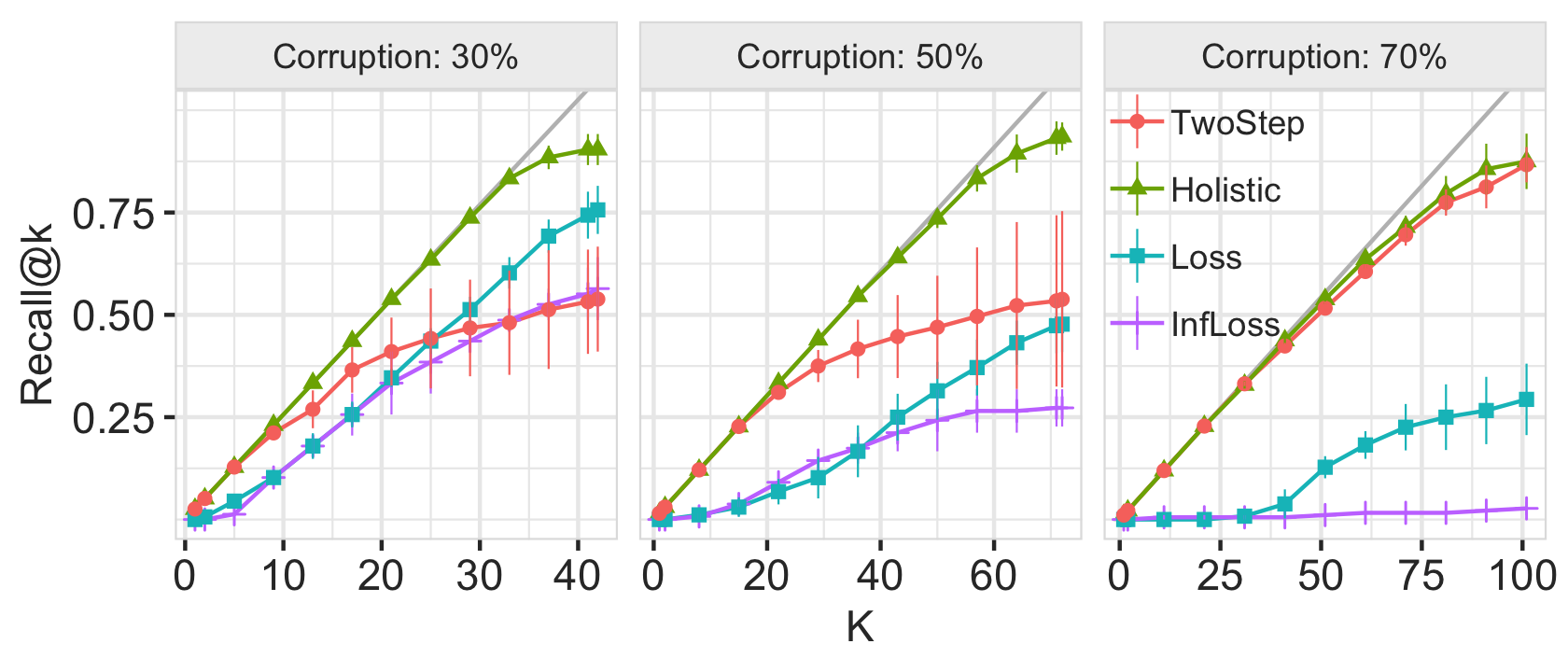
Figure 3. Recall curves when varying corruption rate for DBLP (grey line is perfect recall). Loss-based approaches perform poorly as corruption rate increases, while TwoStep improves at very high corruption rates (70%). Holistic dominates the other approaches.

Figure 3 shows the recall curves for low (30%), medium (50%), and high (70%) corruption rates, where the grey line is a reference for perfect recall. Both loss-based approaches (Loss, InfLoss) degrade substantially as the corruption rate increases because the model begins to overfit to the training corruptions instead. This is corroborated by Figure 5. There we observe the F1 score of the model, the geometric mean of the model precision and recall, on the querying set as the corruption rate increases. For small corruption rates, the model treats the few corruptions as outliers and it does not fit them leading to robust performance. However, this changes for corruption rates larger than $50\%$ where performance starts to drop drastically indicating that the model has started fitting to the corrupted data. TwoStep initially performs poorly, but improves as the systematic errors dominate the training set ($70\%$) and reduce the complaint ambiguity. In contrast, Holistic is nearly perfect, and is robust to the different corruption rates. For reference, the $AUC_{CR}$of the approaches for medium corruption are shown as the first row in Table 3.

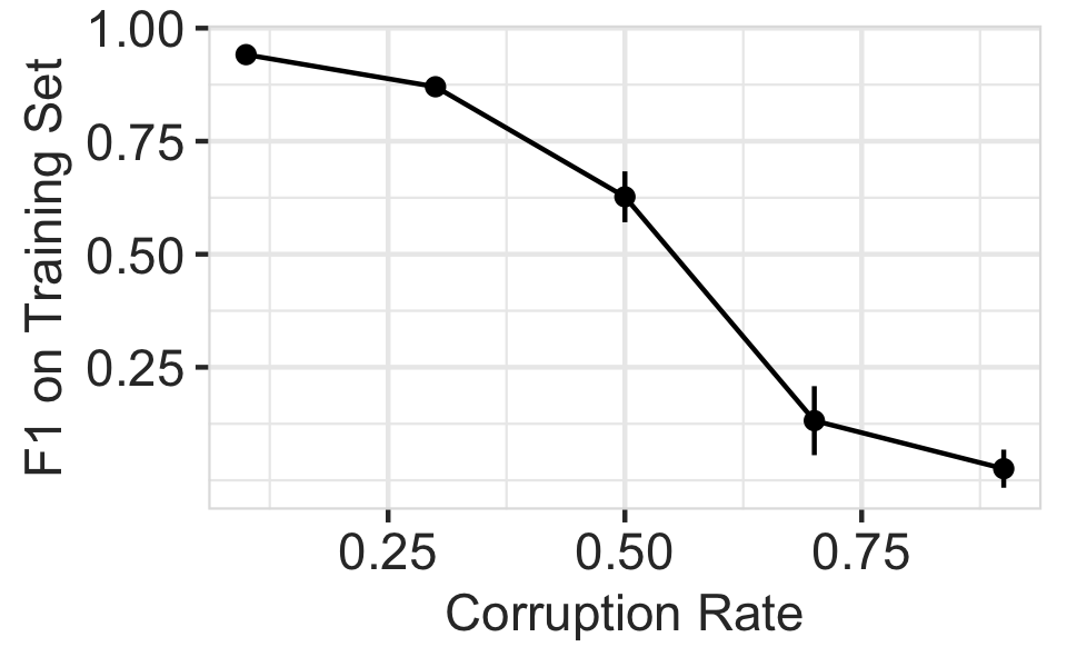
Figure 4. F1 vs corruption rate on DBLP

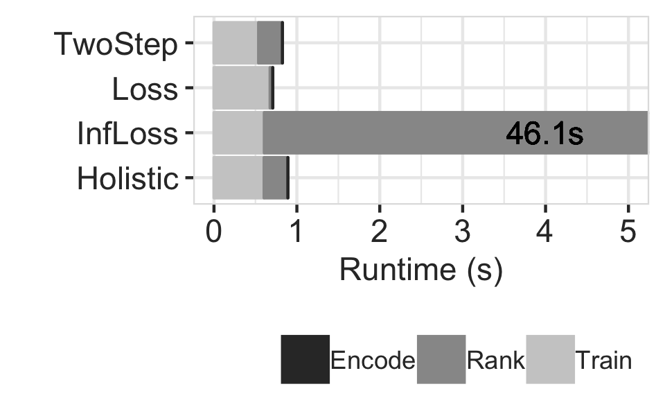
Figure 5. Per-iteration runtime on DBLP, 50% corruption. InfLoss takes 46.1s.

Figure 5 shows the runtime for each train-rank-fix iteration. We report three values, based on the terms in Equation 4. Train refers to model retraining to compute the model parameters $\boldsymbol{\theta}^{*}$; Encode refers to the cost of computing the influence function $-\nabla_{\boldsymbol{\theta}}q(\boldsymbol{\theta}^{*})$; Rank refers to evaluating $\nabla_{\boldsymbol{\theta}}q(\boldsymbol{\theta}^{*})H_{\boldsymbol{\theta}^{*}}^{-1}$, which is dominated by calculating the Hessian vector products required by the conjugate gradient approach of (Martens, 2010). Loss is the fastest because it simply uses the training loss and avoids costly influence estimation; InfLoss has similar or worse recall curves than Loss, but is by far the slowest because it computes a unique influence function for each training record. Holistic and TwoStep are comparable, and dominated by the ranking cost.

We next evaluate the ENRON dataset using $Q_{2}$, where the search word in the LIKE predicate is either ‘http’ or ‘deal’. The corruptions simulate rule-based labeling functions. For the ‘http’ query, we label all training emails containing ‘http’ as spam (13% of emails, of which 76% already labeled spam). The label corruption method is similar for the ‘deal’ query (18% of emails, 2.7% labeled spam). Table 3 summarizes the results: InfLoss, Loss and TwoStep perform poorly. It is worth pointing out that InfLoss takes 2 days to produce the results. Holistic performs much better for ‘deal’ because 17.5% more training labels were flipped, in contrast to only 3.14% for ‘http’.

Dataset		InfLoss	Loss	TwoStep	Holistic
DBLP		0.30	0.35	0.71	0.99
ENRON	’%http%’	0.05	0.02	0.04	0.12
ENRON	’%deal%’	0.17	0.02	0.07	0.40

Table 3. AUC for DBLP with medium corruption, and ENRON with different search words.

Takeaways: Loss-based approaches are sensitive to the number of systematic errors in the training set—at large corruption rates, the model can overfit to the errors and lead to poor debugging quality. In contrast, complaints help ensure training records are ranked according to their effects on the complaints. We find that InfLoss takes over 40s per iteration, yet performs poorly under systematic errors. For these reasons, we do not evaluate InfLoss in subsequent experiments, but keep Loss to serve as a comparison point.

6.3. Baseline Comparison: SPJA Queries

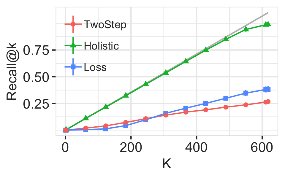
(a) Recall for point complaints (50% corruption).

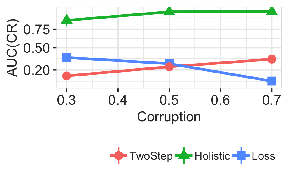
(b) $AUC_{CR}$for point complaints.

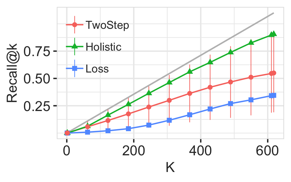
(c) Recall for COUNT complaint (50% corruption).

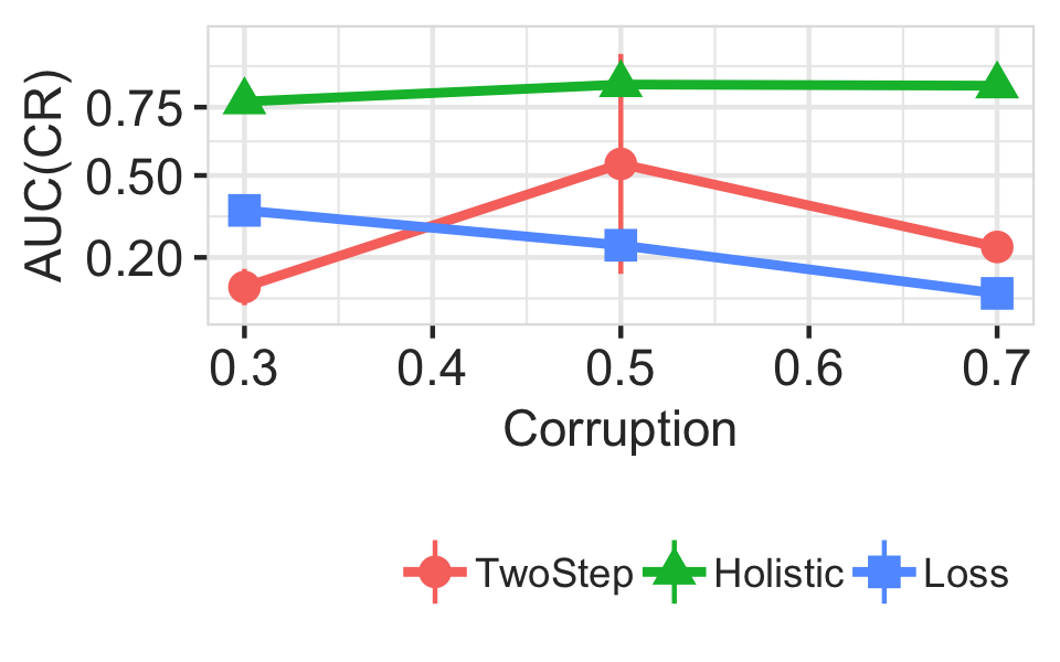
(d) $AUC_{CR}$for COUNT complaint.

Figure 6. MNIST complaints on individual join rows (a-b), or COUNT of join results (c-d).

This section uses the MNIST dataset to evaluate complaint-based debugging against the baselines for SPJA queries containing joins. The first two experiments join two image subsets that do not overlap in their digits, and thus expect no results of the join operation. We introduce corruptions by flipping a random subset of digit $1$ images to be labeled $7$ instead. We corrupt 30% (low), 50% (medium), and 70% (high) of the labels, impacting 3%, 5% and 7% of the total training labels accordingly. We chose MNIST to make the problem more ambiguous: the model is a 10-digit classifier, thus there are 10 ways ($1=1$, $2=2$, e.t.c.) to incorrectly satisfy the join condition, but 90 ways to incorrectly fix it (all other label combinations). We thus expect TwoStep to perform poorly due to a large number of satisfying, but incorrect, ILP solutions.

We first use $Q_{3}$, which joins images of $1$ with images of $7$. We generate tuple complaints for join results where the left (or right) side of the join was correctly predicted, but the right (left) side was incorrect. This results in 121, 550, and 931 complaints for the low, medium, and high corruption rates. Figure 6(a) shows that TwoStep and Loss perform poorly compared to Holistic, despite 550 complaints. When varying the corruption rate in Figure 6(b), TwoStep improves slightly, but is still dominated by Holistic.

Our second experiment runs a COUNT aggregation ($Q_{4}$) on $Q_{3}$’s results. The left relation contains images with digits $1$ through $5$; the right relation contains digits $6-9,0$. The complaint says that the result should be $0$—this is the same as a delete complaint on all join tuples, and states that all left tuples should not have the same prediction as any in the right relation. As expected, the lower ambiguity improves the likelihood that TwoStep’s ILP picks a good satisfying solution, but the large standard deviation shows that it is unstable (Figure 6(a)). Figure 6(d) shows both Loss and TwoStep perform poorly across corruption rates; note that TwoStep is erratic between runs and doesn’t show a clear trend.

Our third experiment joins two image datasets that overlap. We use the same relations as the previous experiment, and set the corruption rate to 50%. However, we move a subset of the $1$ digit images from the left relation to the right, which we call the mix rate. For example, a mix rate of 25% means that we move 25% of the $1$ images ($296$ out of 1125) from the left relation to the right—the true output of $Q_{4}$ should be $829\times 296=245384$, whereas the incorrect output was $1044470$. As noted in Section 5.2.2, this is far more ambiguous than the previous experiment. As we vary the mix rate between $5\%$, $25\%$, $35\%$, the $AUC_{CR}$for Loss is stable at $\approx 0.24$, whereas Holistic is initially high then decreases slightly ($AUC_{CR}$$=0.78,0.57,0.48$, respectively). TwoStep does not solve the ILP within $30$ minutes, thus we cannot report its results.

Takeaways: Overall, Holistic achieves the highest recall on SPA and SPJA queries as compared to the baselines as well as TwoStep. TwoStep is sensitive to the ILP solver as well as the level of ambiguity, which we will evaluate in the next subsection.

6.4. Effects of Ambiguity

The previous experiments suggested the effects of high ambiguity on the different approaches. In this experiment, we use the same setup as $Q_{3}$ in the SPJ experiment, and carefully vary the amount of complaint ambiguity. In the previous experiment, the complaint only specifies that the join output record should not exist, but does not prescribe how to fix it. Here, we will replace a subset $\alpha$ of those complaints with unambiguous complaints. Specifically, for a complaint over a join output record $(l\in L,r\in R)$, we replace it with value complaints on the output of the model predictions $predict(l)$ and $predict(r)$. We corrupt 30% of the $1$ digits as in the previous experiment.

Figure 7 shows that Holistic dominates the approaches at high ambiguity (10% complaints), however at low ambiguity (80%), TwoStep is competitive with Holistic. In addition, this experiment illustrates how Rain can make use of complaints from different parts of the query plan. Specifically, we can view the join record complaints as complaints on the output of $Q_{3}$ and the unambiguous complaints on the predictions of $L$ and $R$ as complaints that target the provenance of $Q_{3}$.

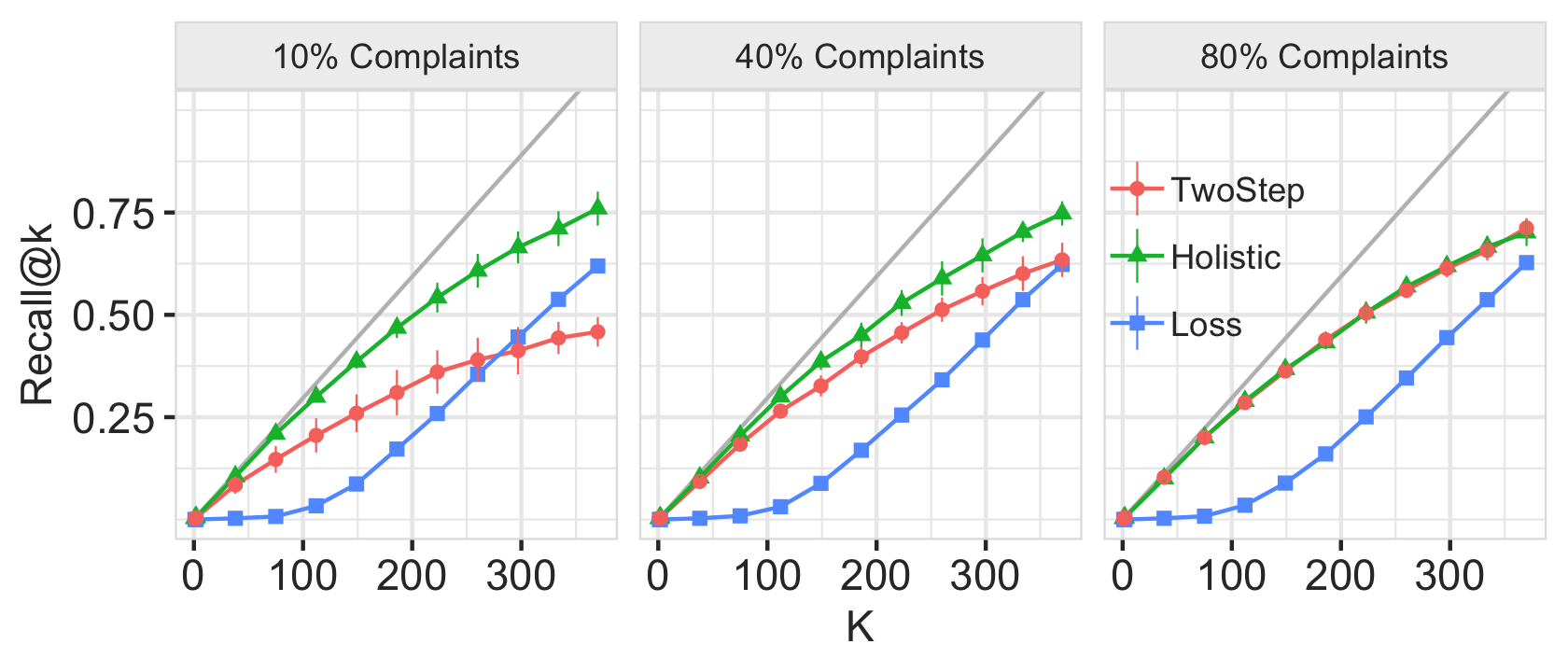
Figure 7. Varying ambiguity of the MNIST point complaints experiment. Each facet varies the percentage of join result complaints that are replaced with direct complaints over the model mispredictions.

Takeaways: TwoStep is sensitive to ambiguity. TwoStep converges to Holistic when ambiguity is reduced by, for example, directly labelling many model mispredictions.

6.5. Multi-Query Complaints

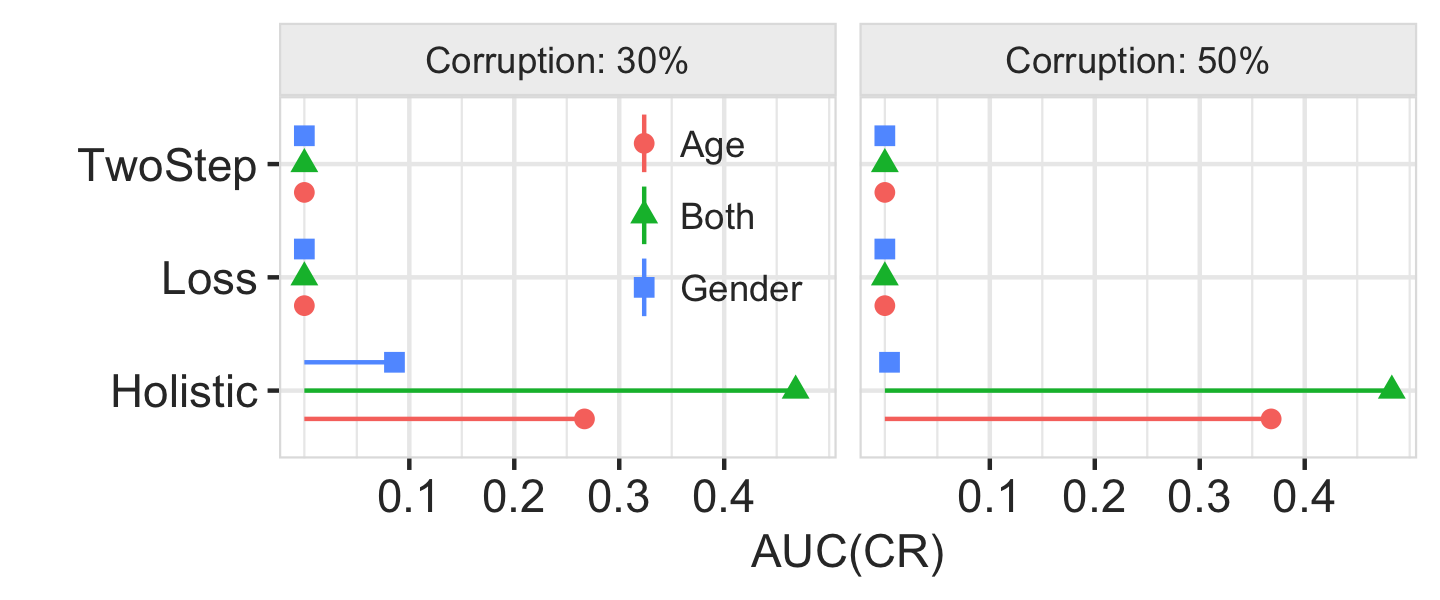
Figure 8. Holistic can benefit from combining complaints of multiple queries.

So far, we have evaluated Rain using a single query and on a single attribute. In this experiment, we use the multi-attribute Adult dataset, and illustrate that complaints over different queries (that use the same model) can be combined to more effectively identify training set errors. We execute $Q_{6}$ and $Q_{7}$ from Table 2. $Q_{6}$ groups the dataset by Gender and creates a value complaint for the male average value. $Q_{7}$ aggregates the dataset by Age (bucketed into decades), and creates a value complaint for the 40-50 age group’s average value. To corrupt the training set, we select records that satisfy the conjunction of low income, male, and 40-50 years old, and flip $\alpha\%$ of their labels from low income (y=0) to high income (y=1). $8.2\%$ of the training set matches this predicate. We set $\alpha\in\{30\%,50\%\}$ thus affecting the labels of $2.4\%$ and $4.1\%$ training points respectively.

Figure 8 shows that TwoStep, Loss, and Holistic when given each complaint in isolation, and when given both. TwoStep and Loss are unable to find any erroneous training records. One of the reasons is that the preprocessing step borrowed from  (du Pin Calmon et al., 2017) only uses three attributes to construct their features. This results in many duplicate training points (118/6512 points are unique). Thus, considerably more iterations for TwoStep and Loss are spent proposing and removing duplicates. Further, TwoStep’s SQL step is agnostic to the model and training set, and fails to leverage this information when solving the ILP.

Holistic is, to a lesser degree, affected by the duplicates for the Gender complaint. This is because Gender is less selective than Age: in the training set, only $23.1\%$ of males are between 40 and 50 but $71.3\%$ of people between 40 and 50 are males. Holistic benefits considerably from using both complaints because they serve to narrow the possible training errors to those within the corrupted subspace.

Takeaways: Users often run multiple queries over the same dataset. We find that Holistic is able to leverage complaints across multiple queries. In contrast, techniques that are oblivious to the complaints (Loss) or oblivious to the model and training (TwoStep) perform poorly.

6.6. Do Complaints Reduce Debugging Effort?

One of the potential benefits of a complaint-based debugging approach is that users can specify a few aggregate but potentially ambiguous complaints, rather than label many individual, unambiguous, model predictions. In addition, it is desirable that complaints are robust to mis-specifications. For example, if a result value is 20 but should be 49, then a value complaint that is $50$, or $60$, or $45$ should not greatly affect the returned training records. We now evaluate both of these questions in sequence. We use the MNIST dataset with corruptions that flip 10% of the training images with the digit $1$ to be labeled $7$.

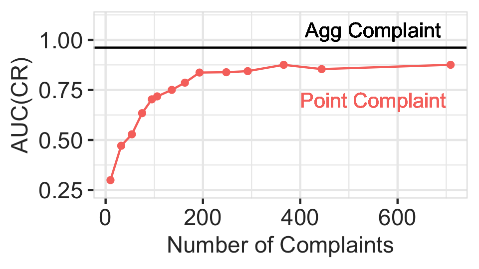
Figure 9. Comparison of one aggregate complaint (black) and increasing the number of point complaints (red)

First, we compare aggregate-level and prediction-level complaints. Agg Complaint is a single value complaint over $Q_{5}$, which counts the number of $1$ digits; Point Complaints varies the number of complaints of model mispredictions from 1 to 709, and is equivalent to state-of-the-art influence analysis (Koh and Liang, 2017)). Figure 9 shows that the aggregate complaint is enough to achieve $AUC_{CR}$$\approx 1$, whereas TwoStep requires over $200$ point complaints to reach $AUC_{CR}$$\approx 0.87$. This suggests that, from an user perspective, aggregate-level complaints can require less effort.

A potential drawback of aggregate-level complaints is that they may be sensitive to mis-specification. To evaluate this, we introduce three types of errors to the user’s value complaint. The errors vary in the user-specified $X$ in the equality complaint $t[a]=X$, as compared to the ground truth $X^{*}$. Overshoot overcompensates for the error by setting $X=1.2\times X^{*}$, meaning if the query result was $10$ and the ground truth was $100$, then $X$ is set to $120$. Partial under-estimates the error but correctly identifies the direction the query result should move—$X$ is set to the average of the query result and the ground truth (e.g., $55$ in the preceding example). Wrong overcompensates in the incorrect direction, and sets $X=0.8\times t[a]$.

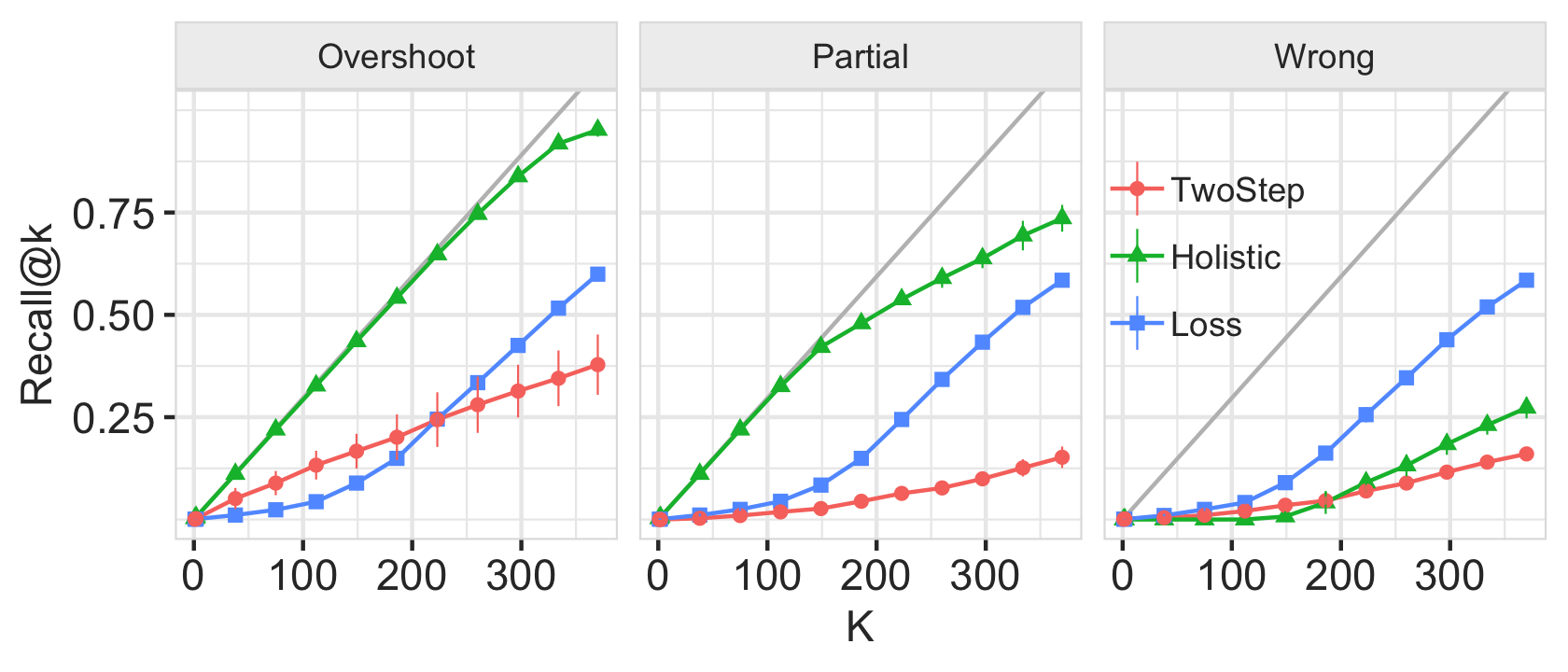
Figure 10. How errors in complaints affect each approach.

Figure 10 shows that Holistic is relatively robust to misspecified complaints, as long as they point in the correct direction of error. Specifically, the HolisticPartial curve degrades around $K=150$ because the complaint has been satisfied. Holistic performs poorly when the complaint direction is Wrong because it tries to identify training records that if removed reduce the count whereas the true corruptions do the opposite. TwoStep similarly degrades, whereas Loss is insensitive because it does not rely on complaints at all.

Takeaways: Complaint-based approaches allow users to provide few ambiguous complaints over aggregated results, and still accurately identify training set errors. Holistic is robust to misspecifications as long as the direction of the complaint is correct.

7. Related Work

Rain provides complaint-driven data debugging for relational queries that use machine learning inference. This is most closely related to SQL explanations in the DB community, ML explanations in the ML community. It is also related to data cleaning for machine learning, as well as debugging ML pipelines in general.

SQL Explanation: SQL explanation seeks to explain errors in a query result. Errors may be specified as incorrect values, how values should change, tuples that should not exist, or tuples that should exist. These errors can be explained as subsets of the queried relations (Kanagal et al., 2011), predicates over the queried relations that should be deleted (Wu and Madden, 2013; Roy et al., 2015; Abuzaid et al., 2018; Roy and Suciu, 2014), values of the queried relations that should be changed (Meliou and Suciu, 2012), changes to the query (Chapman and Jagadish, 2009; Tan et al., 2017; Tran and Chan, 2010), or changes to past queries (Wang et al., 2017). This line of work is generally related to causal interventions in queries (Meliou et al., 2014; Salimi et al., 2018) and reverse data management (Meliou et al., 2011).

Provenance (Kanagal et al., 2011; Green et al., 2007; Dalvi and Suciu, 2004) returns the queried records, and how they were combined, for a given output record. This is a form of explanation, serves as the starting point for many of the SQL explanation approaches above, including this work. From our perspective, Rain traces user complaints back through the query, and by using influence analysis, back to the training records.

ML Explanation: Gilpin et. al (Gilpin et al., 2018) provide an excellent survey of ML Interpretation. A major aspect of ML explanation is in understanding why a model makes a specific prediction for a data point, and techniques include surrogate models (Ribeiro et al., 2016), saliency maps (Simonyan et al., 2013; Zeiler and Fergus, 2014; Shrikumar et al., 2017), decision sets (Lakkaraju et al., 2016), rule summaries (Ribeiro et al., 2018; Krishnan and Wu, 2017), hidden unit analysis (Sellam et al., 2019), sensitivity analysis (Kantchelian et al., 2016; Nilforoshan and Wu, 2017), and general feature attribution methods (Sundararajan et al., 2017; Lundberg and Lee, 2017).

Most related are case-based explanations that identify training records that affected a set of mispredictions. Of these, influence analysis methods are prominent. Techniques such as DUTI (Zhang et al., 2018) model this task as a bi-level optimization problem that may require several rounds of model retraining to identify a single training point. Influence Functions (Koh and Liang, 2017) avoid retraining by approximating this influence locally.

The limitation of these approaches is that they assume that the user has identified model mispredictions. In contrast, Rain focuses on query result complaints that have been affected by model mispredictions. However, it may not be directly known which of the queried records have been mispredicted.

Debugging ML Pipelines: Relational plans, such as those studied in this work, can be viewed as a restricted form of general data analysis pipelines. Within this context, data errors are a major issue in ML pipelines (Polyzotis et al., 2017). Systems such as Data X-Ray (Wang et al., 2015) help debug large-scale data pipelines by summarizing data errors that share a common cause. Data validation (Breck et al., 2019; Shawi et al., 2019) and model assertions (Kang et al., 2020) help catch errors before deployment. This work relies on record-level provenance to address complaints; provenance is increasingly viewed as an integral part of any modern ML pipeline (Varma et al., 2018; Agrawal et al., 2019).

Data Cleaning: Machine learning relies on training data. Data cleaning is both used to clean errors in training datasets to improve ML models, and leverage ML to identify errors. Traditional data cleaning is largely based on constraints (Rahm and Do, 2000; Chu et al., 2013). In contrast, recent work leverages knowledge of downstream ML models (Krishnan et al., 2016; Krishnan et al., 2017; Krishnan and Wu, 2019; Li et al., 2019b), integrates cleaning signals from heterogeneous sources (Rekatsinas et al., 2017), and leverages machine learning to perform error detection (Heidari et al., 2019; Mahdavi et al., 2019; Abedjan et al., 2016).

In addition to general methods for addressing noisy labels (Frénay and Verleysen, 2013), techniques such as Snorkel help identify conflicting and noisy labels from different labeling sources (Ratner et al., 2017), while other work leverages oracles (Dolatshah et al., 2018).

Unlike the existing studies in data cleaning, our work is focused on detecting training set errors w.r.t. the user complaints expressed as Query 2.0.

8. Conclusions and Discussion

Leveraging model inference within query execution (which we call Query 2.0) is rapidly gaining wide-spread adoption. However, query results are now susceptible to errors in the model’s training data. Although there exist techniques to individually debug outliers of SQL queries, and prediction errors in ML models, techniques to address the combination of the two do not exist.

To this end, Rain helps users identify training set errors by leveraging not only the model and data, but also user complaints about final or intermediate query results. Rain integrates these together to find the training records that will most address the user’s complaints. To do so, we introduce two approaches. TwoStep splits the query into SQL-only and ML prediction-only subplans that can be solved using existing SQL and ML explanation techniques. Holistic is an optimization that integrates both steps to directly estimate each training record’s influence on user complaints. Our experiments show that Holistic more accurately identifies systematic training set errors as compared to existing ML explanation techniques, across relational, image, and text datasets; linear and neural network models; and different SPJA queries.

Other Interventions: The type of intervention for fixing the training data is not restricted to only the deletion. Existing techniques like (Tanaka et al., 2018) advocates doing label fixing while training and others like (Krishnan et al., 2016) proposes both feature and label fixing. Rain chooses deletion based intervention for two reasons: 1. Deletion based intervention is a natural and wide used in SQL explanation (Wu and Madden, 2013). Rain uses deletion as the first step towards this broader Query 2.0 Debugging problem, 2. There can be many choices to fix the labels, even more for features. It is unclear how to find the correct fix. We leave other interventions as the future work.

Systematic Debugging: Combining separate analysis methods in a piece-wise manner, such as TwoStep, can perform poorly. This is both because errors from one step will propagate and affect subsequent steps, and because information cannot be shared between steps. Holistic suggests that it is important to consider the entire pipeline and user specifications in a holistic manner.

Stepping back, there is an increasing need for system-wide debugging of data analytic pipelines that use model inference. This paper advocates for a complaint-driven approach towards pipeline debugging. Different users—customers, engineers, data scientists, and ML experts—have differing access, perspective, and expertise of the data that flows through these analytic pipelines (Baylor et al., 2017; Polyzotis et al., 2017). We plan to extend this work beyond SPJA queries to general relational and non-relational workflows, to improve the runtime of the system, and to study interventions beyond training record deletion.

Appendix A Ambiguity & TwoStep

In this section, we will describe a setting where TwoStep is unlikely to identify the correct training errors because the complaint is ambiguous. Specifically, we will formally prove that very few solutions to the SQL step of TwoStep can lead to a training error discovery in the influence step.

For the needs of our setting, we will focus on debugging a binary logistic regression model $M$. Its training set $T$ consists of data that is drawn from a clean distribution as well as a single noisily labeled example $\boldsymbol{t}$. Let $l^{\prime}\in\{0,1\}$ be the noisy label of $\boldsymbol{t}$. For convenience, let the feature vector of $\boldsymbol{t}$ be orthogonal to the other records in $T$, i.e. its inner product with all other feature vectors is zero. Symmetrically, the queried records distribution contains $n$ records with all but $m$ being orthogonal to $\boldsymbol{t}$, just like the clean distribution. The remaining $m$ records can be arbitrary.

Let the query $Q$ count the number of records in the queried dataset where $M.predict(r)=1-l^{\prime}$, the opposite of the $\boldsymbol{t}$’s incorrect label. The user complaint is that the query result should be $k$ when the current result is $0$. We use TwoStep with an influence analysis step based on (Koh and Liang, 2017).

Theorem A.1.

Assuming that the ILP solver picks uniformly at random from the satisfying solution space, then for fixed $m,k$ the probability that TwoStep assigns $\boldsymbol{t}$ a non-zero score in the influence analysis step converges to $0$ as $n\to\infty$.

The intuition of the proof is straightforward. Given the orthogonality condition, the predictions of the $n-m$ queried records coming from the clean distribution would be the same regardless if $\boldsymbol{t}$ existed or not. Unless the ILP assignment picks at least one of the remaining $m$ records, influence analysis at the second step will always assign a zero score for $\boldsymbol{t}$. As $n$ increases with $k$ and $m$ fixed the probability of picking even one of the $m$ records decreases to 0.

For each of the ILP solutions that do not favor the recovery of $\boldsymbol{t}$, we can always construct clean training records with positive scores that are ranked above $\boldsymbol{t}$. Injecting as many as we want for each ILP solution, we can guarantee that TwoStep ranks $\boldsymbol{t}$ arbitrarily low. We will conclude this section with the proof of the main theorem.

Proof.

Let $\boldsymbol{\theta}$ be the parameters of the logistic regression problem. We can write

$$\boldsymbol{\theta}=\boldsymbol{\theta}_{\textrm{noise}}+\boldsymbol{\theta}_{\textrm{clean}}$$

where $\boldsymbol{\theta}_{\textrm{noise}}$ is the projection of $\boldsymbol{\theta}$ on the direction of the feature vector of $\boldsymbol{t}$ and the second term is the orthogonal residue. We will call $\boldsymbol{v}_{\textrm{noise}}$ the feature vector of $\boldsymbol{t}$ and $\boldsymbol{v}_{i}$ and $y_{i}$ the feature vectors and labels of the clean data. Let $\ell$ be the sample loss function of $M$

$$L(\boldsymbol{\theta})=\sum_{i=1}^{T_{c}}\ell(\boldsymbol{v}_{i},y_{i},\boldsymbol{\theta})+\ell(\boldsymbol{v}_{\textrm{noise}},l^{\prime},\boldsymbol{\theta})+\lambda\left\lVert\boldsymbol{\theta}\right\rVert^{2}$$

where the first term corresponds to the loss of the clean data and the second term corresponds to the loss of $\boldsymbol{t}$. $\ell$ takes the feature vector and projects it to $\boldsymbol{\theta}$ and then applies the sigmoid function and then the log loss. Let $f$ denote the function implementing the steps after the projection

$$\ell(\boldsymbol{\theta},\boldsymbol{v}_{i},y_{i}) =f(\boldsymbol{\theta}\cdot\boldsymbol{v}_{i},y_{i})=f(\boldsymbol{\theta}_{\textrm{clean}}\cdot\boldsymbol{v}_{i},y_{i})$$

$$\ell(\boldsymbol{\theta},\boldsymbol{v}_{\textrm{noise}},l^{\prime}) =f(\boldsymbol{\theta}\cdot\boldsymbol{v}_{\textrm{noise}},l^{\prime})=f(\boldsymbol{\theta}_{\textrm{noise}}\cdot\boldsymbol{v}_{\textrm{noise}},l^{\prime})$$

That is the clean distribution loss depends only on $\boldsymbol{\theta}_{\textrm{clean}}$ and the loss on $\boldsymbol{t}$ depends only on $\boldsymbol{\theta}_{\textrm{noise}}$. Thus we essentially have two loss functions that depend on disjoint variables

$$L(\boldsymbol{\theta}) =\sum_{i=1}^{T_{c}}f(\boldsymbol{\theta}_{\textrm{clean}}\cdot\boldsymbol{v}_{i},y_{i})+\lambda\left\lVert\boldsymbol{\theta}_{\textrm{clean}}\right\rVert^{2}$$

$$+f(\boldsymbol{\theta}_{\textrm{noise}}\cdot\boldsymbol{v}_{\textrm{noise}},l^{\prime})+\lambda\left\lVert\boldsymbol{\theta}_{\textrm{noise}}\right\rVert^{2}$$

$$=L_{1}(\boldsymbol{\theta}_{\textrm{clean}})+L_{2}(\boldsymbol{\theta}_{\textrm{noise}})$$

Essentially we have two distinct optimization problems

$$\boldsymbol{\theta}_{\textrm{clean}}^{*} =\operatorname*{arg\,min}_{\boldsymbol{\theta}_{\textrm{clean}}}L_{1}(\boldsymbol{\theta}_{\textrm{clean}})$$

$$\boldsymbol{\theta}_{\textrm{noise}}^{*} =\operatorname*{arg\,min}_{\boldsymbol{\theta}_{\textrm{noise}}}L_{2}(\boldsymbol{\theta}_{\textrm{noise}})$$

Observe that the existence of $\boldsymbol{t}$ does not affect the value of $\boldsymbol{\theta}_{\textrm{clean}}^{*}$. Additionally, predictions on queried records that have feature vectors that are orthogonal to $\boldsymbol{t}$ depend only on $\boldsymbol{\theta}_{\textrm{clean}}^{*}$. Thus complaints on these queried records cannot be resolved by deleting $\boldsymbol{t}$. For these complaints, $\boldsymbol{t}$ would be assigned a zero score by the influence step of TwoStep.

The feature vectors of the $m$ queried records are the only ones that could have a non-zero inner product with $\boldsymbol{t}$. Thus, out of all the satisfying solutions of the ILP, only ones that assign the label of $1-l^{\prime}$ to at least one of the $m$ queried records has any hope of giving $\boldsymbol{t}$ a non-zero score in the influence analysis step. Observe that there are $\binom{n}{k}$ solutions to the ILP and there are $\binom{n-m}{k}$ assignments that do not pick any of the $m$ points. The probability of picking such an assignment is converging to 1.

$$\lim_{n\to\infty}\frac{\binom{n-m}{k}}{\binom{n}{k}} =\lim_{n\to\infty}\frac{(n-m)!(n-k)!}{(n-m-k)!n!}$$

$$=\lim_{n\to\infty}\prod_{i=0}^{k-1}\frac{n-i-m}{n+i}=1$$

The probability of assigning $\boldsymbol{t}$ a non-zero score goes to 0. ∎

Appendix B Holistic Relaxation Examples

In this section, we will provide additional examples of how Holistic handles multi-class classification models and aggregate comparisons in SQL queries.

Multi-class models Relaxing SQL queries that use multi-class classification models is also supported. As an example, let us consider the MNIST dataset that we describe in Section 6. We can design a classifier that takes one image, represented by a $28\times 28$ grid of pixels, and yields a number from $0$ to $9$ corresponding to the digit displayed. We may want to use this model in an optical character recognition application that takes a handwritten multi-digit number, segments it into small images each containing a single digit and uses the classifier to figure out the numerical value of the whole number. Let us assume that the segmentation has occurred and that we have the sequence of $N$ images stored in a table DIGITS in an attribute called image. Along with each image we have a field position indicating the digit position from the right. The numeric value of the number is represented in SQL by the following query

$${\footnotesize\textsf{SELECT SUM(POWER(10, position)*predict(image)) FROM DIGITS}.}$$

Let $\boldsymbol{\theta}$ be the parameters of our model and $p_{ij}(\boldsymbol{\theta})$ be the probability assigned by the classifier that the image at position $i$ is digit $j$. Then the relaxation of the query output is the following quantity

$$\sum_{i=1}^{N}10^{i-1}\sum_{j=0}^{9}j\cdot p_{ij}(\boldsymbol{\theta})$$

Aggregate comparisons SQL queries are allowed to use comparisons in their selection and join predicates. Unfortunately, the relaxation rules for Holistic as described in Section 5.3 do not directly support comparison operators. Regardless of its complexity, every comparison has an equivalent logical formula involving only $\texttt{AND},\texttt{OR},\texttt{NOT}$ that Holistic supports. Finding such a logical formula can be non-trivial when aggregate values are compared. SQL can express aggregate comparisons through a HAVING clause.

For example, let us revisit the optical character recognition application of the previous subsection. We want to express a predicate selecting numbers that are greater or equal than $95$. Let $x_{i,j}$ be the boolean value expressing that the digit at position $i$ from the right is classified as being $j$. For simplicity we focus on the case of two-digit numbers. Then the aggregate comparison is equivalent to the following formula

$$x_{2,9}\texttt{ AND }\left(\bigvee_{9\geq\ell\geq 5}x_{1,\ell}\right)$$

In general, finding the equivalent formula can be a computationally expensive procedure and the resulting formula can have a large amount of terms slowing down the influence analysis step. Identifying ways to relax comparisons directly is a promising direction for future work. It is important to note that comparisons that are part of the complaint itself do not require special care. They can be handled directly based on the techniques described in Section 5.3.

Appendix C The value of complaints

In this section, we will describe a setting where ordering training records based on loss or loss sensitivity ranks training corruptions at the bottom. At the same time, an appropriately selected complaint is sufficient to rank all corrupted training records at the top.

For the needs of our setting, we will focus on debugging a binary logistic regression model $M$. Our training set $T$ is a mixture of clean and corrupted training records. Clean records have been perfectly labelled whereas the corrupted ones have had theirs inverted. Corrupted training records labelled as being in class $1$ are truly in class $0$ and vice versa.

For simplicity, we are going the two following assumptions. First, the feature vectors of the clean training records are all orthogonal to the ones in the corrupted distribution. That is for each pair of records from the two distributions, the corresponding feature vectors have zero inner product. Second, the feature vectors for all corrupted training records are parallel. That is for each pair of feature vectors $\boldsymbol{v}_{i}$ and $\boldsymbol{v}_{j}$ from the corrupted training records, there is a $\kappa_{ij}\in\mathbb{R}$ such that $\boldsymbol{v}_{i}=\kappa_{ij}\boldsymbol{v}_{j}$. Third, we are going to assume that the corrupted training records are linearly separable, i.e. there is a linear classifier that can correctly specify the labels of the corrupted training records.

Let us discuss the two ways we can use the model loss to rank training records. The first one is to use the loss value of each training record. The Loss baseline discussed in the experiments ranks training records with higher loss at the top. The second one ranks training records based on loss sensitivity. Specifically, (Koh and Liang, 2017) considers the effect of the removal of each training record on its own loss. This is the InfLoss baseline. For each training record $\boldsymbol{z}$ it computes a loss sensitivity

$$-\nabla_{\boldsymbol{\theta}}\ell(\boldsymbol{z},\boldsymbol{\theta}^{*})H_{\boldsymbol{\theta}^{*}}^{-1}\nabla_{\boldsymbol{\theta}}\ell(\boldsymbol{z},\boldsymbol{\theta}^{*}).$$

These scores are negative or zero since the Hessian of logistic regression, and thus its inverse, is positive definite. Large negative values indicate that when the training record is removed, its own loss tends to increase rapidly. These training records are ranked at the top by InfLoss. The following holds

Theorem C.1.

As the number of corrupted training records goes to infinity, the loss and loss sensitivity of corrupted training records goes to zero.

Observe that $0$ is the minimum value of the loss and maximum value of the loss sensitivity. Thus both approaches rank corrupted training records at the bottom. As a first step let us prove this theorem.

Proof.

Let $\boldsymbol{\theta}$ be the parameters of the logistic regression problem. We can once again write

$$\boldsymbol{\theta}=\boldsymbol{\theta}_{\textrm{noise}}+\boldsymbol{\theta}_{\textrm{clean}}.$$

$\boldsymbol{\theta}_{\textrm{noise}}$ is the projection of $\boldsymbol{\theta}$ on the direction of the feature vector of a corrupted training record. It does not matter which one since all are parallel. $\boldsymbol{\theta}_{\textrm{clean}}$ is the orthogonal residue.

We can apply the same techniques as in the proof of Theorem A.1 to get two independent optimization problems. Let $K$ be the number of corrupted points, $\boldsymbol{v}_{i}$ the feature vectors and $y_{i}$ the corresponding corrupted labels. Using the $f$ function from the proof of Theorem A.1

$$\boldsymbol{\theta}_{\textrm{noise}}^{*}=\operatorname*{arg\,min}_{\boldsymbol{\theta}_{\textrm{noise}}}\left(\sum_{i=1}^{K}f(\boldsymbol{v}_{i}\cdot\boldsymbol{\theta}_{\textrm{noise}},y_{i})+\lambda\left\lVert\boldsymbol{\theta}_{\textrm{noise}}\right\rVert^{2}\right)$$

As a first step we want to prove that

$$\lim_{K\to\infty}f(\boldsymbol{v}_{i}\cdot\boldsymbol{\theta}_{\textrm{noise}}^{*},y_{i})=0$$

for all pairs of $\boldsymbol{v}_{i}$ and $y_{i}$ from the corrupted training records. This states that the loss of the corrupted records goes to 0, our first claim. Let $\sigma$ be the sigmoid function. By first order conditions we have that $\boldsymbol{\theta}_{\textrm{noise}}^{*}$ satisfies

$$\sum_{i=1}^{K}\left(\sigma(\boldsymbol{v}_{i}\cdot\boldsymbol{\theta}_{\textrm{noise}}^{*})-y_{i}\right)\boldsymbol{v}_{i}+2\lambda\cdot\boldsymbol{\theta}_{\textrm{noise}}^{*}=\boldsymbol{0}.$$

We have assumed that the corrupted training records are linearly separable. Thus there exists a vector $\boldsymbol{u}$ that linearly separates the data with margin $1$. Let us multiply with this vector the equation above.

$$\sum_{i=1}^{K}\left(\sigma(\boldsymbol{v}_{i}\cdot\boldsymbol{\theta}_{\textrm{noise}}^{*})-y_{i}\right)\boldsymbol{v}_{i}\cdot\boldsymbol{u}+2\lambda\cdot\boldsymbol{\theta}_{\textrm{noise}}^{*}\cdot\boldsymbol{u}=0.$$

In turn we have that

$$\sum_{i=1}^{K}\frac{\left(\sigma(\boldsymbol{v}_{i}\cdot\boldsymbol{\theta}_{\textrm{noise}}^{*})-y_{i}\right)\boldsymbol{v}_{i}\cdot\boldsymbol{u}}{\boldsymbol{\theta}_{\textrm{noise}}^{*}\cdot\boldsymbol{u}}=-2\lambda.$$

Given that $\boldsymbol{u}$ has margin $1$, we have that

$$(2y_{i}-1)\cdot\boldsymbol{v}_{i}\cdot\boldsymbol{u}\geq 1$$

and thus for both $y_{i}$ equal to $0$ and $1$, all summation terms of the previous equation need to have the same sign. As the number of terms $K$ increases, the terms cannot be bounded away from $0$ while the sum remains finite. Thus $\boldsymbol{\theta}_{\textrm{noise}}^{*}$ is such that either the numerator goes to zero or the denominator goes to infinity or both. In either case

$$\lim_{K\to\infty}\boldsymbol{\theta}_{\textrm{noise}}^{*}\cdot\boldsymbol{u}=\infty$$

Given that all $\boldsymbol{v}_{i}$ are parallel to $\boldsymbol{u}$ and $\boldsymbol{\theta}_{\textrm{noise}}^{*}$, the loss of the samples going to $0$ follows immediately.

Similarly, the gradients of the losses go to a $0$ norm. For the loss sensitivity scores, we have

$$-\nabla_{\boldsymbol{\theta}}\ell(\boldsymbol{z},\boldsymbol{\theta}^{*})H_{\boldsymbol{\theta}^{*}}^{-1}\nabla_{\boldsymbol{\theta}}\ell(\boldsymbol{z},\boldsymbol{\theta}^{*})\geq-\left\lVert\nabla_{\boldsymbol{\theta}}\ell(\boldsymbol{z},\boldsymbol{\theta}^{*})\right\rVert^{2}\lambda_{\textrm{max}}(H_{\boldsymbol{\theta}^{*}}^{-1})$$

where $\lambda_{\textrm{max}}(H_{\boldsymbol{\theta}^{*}}^{-1})$ the biggest eigenvalue of the inverse Hessian. The minimum eigenvalue of the Hessian is at least $2\lambda$. Thus the inverse Hessian has bounded eigenvalues by $\frac{1}{2\lambda}$.

$$-\nabla_{\boldsymbol{\theta}}\ell(\boldsymbol{z},\boldsymbol{\theta}^{*})H_{\boldsymbol{\theta}^{*}}^{-1}\nabla_{\boldsymbol{\theta}}\ell(\boldsymbol{z},\boldsymbol{\theta}^{*})\geq-\left\lVert\nabla_{\boldsymbol{\theta}}\ell(\boldsymbol{z},\boldsymbol{\theta}^{*})\right\rVert^{2}\frac{1}{2\lambda}$$

With the gradient norms going to $0$, the loss sensitivity scores of all corrupted training records need to going to $0$ as well. ∎

Thus for a large enough number of corrupted training records and the clean ones fixed, we can force the corrupted training records to the bottom of the rankings for both Loss and InfLoss. What remains to discuss is how an appropriate complaint can bring these records to the top of the ranks.

Complaints on queried records with feature vectors parallel to the ones of the corrupted training records are particularly interesting. For these complaints, the clean training records receive $0$ influence scores following the same discussion as in Theorem A.1. It thus remains to find one such complaint that assigns positive scores to all corrupted training records.

Even identifying one of the mispredicted queried records that have the property above will do. Let $\boldsymbol{z}_{q}=(\boldsymbol{v}_{q},y_{q})$ be the identified record with its correct label. The influence score of each corrupted training record $\boldsymbol{z}_{i}=(\boldsymbol{v}_{i},y_{i})$ is

$$-\nabla_{\boldsymbol{\theta}}\ell(\boldsymbol{z}_{q},\boldsymbol{\theta}^{*})H_{\boldsymbol{\theta}^{*}}^{-1}\nabla_{\boldsymbol{\theta}}\ell(\boldsymbol{z}_{i},\boldsymbol{\theta}^{*}).$$

We have that

$$\nabla_{\boldsymbol{\theta}}\ell(\boldsymbol{z}_{q},\boldsymbol{\theta}^{*}) =\left(\sigma(\boldsymbol{v}_{q}\cdot\boldsymbol{\theta}_{\textrm{noise}}^{*})-y_{q}\right)\boldsymbol{v}_{q}$$

$$\nabla_{\boldsymbol{\theta}}\ell(\boldsymbol{z}_{i},\boldsymbol{\theta}^{*}) =\left(\sigma(\boldsymbol{v}_{i}\cdot\boldsymbol{\theta}_{\textrm{noise}}^{*})-y_{i}\right)\boldsymbol{v}_{i}.$$

$\boldsymbol{v}_{q}$ and $\boldsymbol{v}_{i}$ are parallel but $\boldsymbol{z}_{q}$ is mispredicted while $\boldsymbol{z}_{i}$ is correctly predicted. Simple algebra shows that the gradients have opposite directions. That is there is a $k>0$ such that

$$\nabla_{\boldsymbol{\theta}}\ell(\boldsymbol{z}_{q},\boldsymbol{\theta}^{*})=-k\nabla_{\boldsymbol{\theta}}\ell(\boldsymbol{z}_{i},\boldsymbol{\theta}^{*})$$

Since the Hessian of logistic regression and thus its inverse is positive definite, we have

$$- \nabla_{\boldsymbol{\theta}}\ell(\boldsymbol{z}_{q},\boldsymbol{\theta}^{*})H_{\boldsymbol{\theta}^{*}}^{-1}\nabla_{\boldsymbol{\theta}}\ell(\boldsymbol{z}_{i},\boldsymbol{\theta}^{*})=$$

$$\quad\quad k\nabla_{\boldsymbol{\theta}}\ell(\boldsymbol{z}_{i},\boldsymbol{\theta}^{*})H_{\boldsymbol{\theta}^{*}}^{-1}\nabla_{\boldsymbol{\theta}}\ell(\boldsymbol{z}_{i},\boldsymbol{\theta}^{*})>0.$$

Thus the influence scores of all corrupted training records are positive and the complaint ranks all of them at the top.

Appendix D Debugging on NN

In this section, we evaluate TwoStep, Loss, and Holistic on a convolutional neural network (CNN) model. We execute the COUNT query $Q_{5}$ on the MNIST dataset, and we corrupt the training set by flipping $50\%$ of the $1$ digit images to be labeled $7$. The CNN model consists of 3-layers (convolution, max pooling, dense with RELU activation). (Koh and Liang, 2017) showed empirically that the influence function analysis works even for neural networks, which are non-convex, including CNN architectures. We also include the logistic regression model for comparison.

This section reports the $AUC_{CR}$for the three approaches. We find that Holistic degrades slightly when debugging the CNN model. This agrees with the findings of (Koh and Liang, 2017), where the influence analysis scores were shown to be less accurate for non-convex than convex models. Recent work on influence analysis (Hara et al., 2019) has provided improved approaches that are more accurate on non-convex models. Rain is compatible with (Hara et al., 2019) and can continue to leverage any improvements on influence analysis by the ML community.

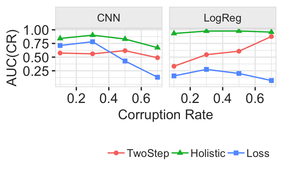
Figure 11. $AUC_{CR}$when using CNN and logistic regression models.

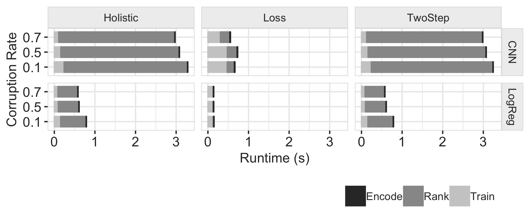
Figure 12. Per-iteration runtimes for debugging CNN and logistic regression models for different corruption rates.

Figure 12 shows that per-iteration runtimes for Loss is dominated by retraining costs. We note that the models are trained incrementally in each iteration i.e. the previous values of the weights are used as initializations for the next debugging iteration. Thus, retraining costs can vary across methods depending on which points are removed. Intuitively removing points with high loss may result in significant model changes and thus can lead to higher retraining costs, explaining the higher retraining time for Loss in Figure 12 when compared to TwoStep and Holistic.

In contrast, TwoStep and Holistic are dominated by calculating the Hessian vector products required by the conjugate gradient approach of (Martens, 2010). Even if the conjugate gradient approach is much faster than naively computing the inverse Hessian, its cost grows linearly with the number of parameters of the model. (Koh and Liang, 2017) suggested doing the influence analysis on neural networks by considering only the weights of the last layer as parameters, treating all the previous layer as a fixed feature transformation. We leave studying the effects of this optimization on debugging runtimes as future work.

Takeaways: Holistic supports queries that use neural network models. It performs well under low and moderate corruption rates and dominates TwoStep and Loss. However, each iteration takes $\approx 3$ seconds due to the cost of the ranking (hessian inverse) step, which is particularly costly for neural network models.

References

- (1)
- Abadi et al. (2015) Martín Abadi, Ashish Agarwal, Paul Barham, Eugene Brevdo, Zhifeng Chen, Craig Citro, Greg S. Corrado, Andy Davis, Jeffrey Dean, Matthieu Devin, Sanjay Ghemawat, Ian Goodfellow, Andrew Harp, Geoffrey Irving, Michael Isard, Yangqing Jia, Rafal Jozefowicz, Lukasz Kaiser, Manjunath Kudlur, Josh Levenberg, Dan Mané, Rajat Monga, Sherry Moore, Derek Murray, Chris Olah, Mike Schuster, Jonathon Shlens, Benoit Steiner, Ilya Sutskever, Kunal Talwar, Paul Tucker, Vincent Vanhoucke, Vijay Vasudevan, Fernanda Viégas, Oriol Vinyals, Pete Warden, Martin Wattenberg, Martin Wicke, Yuan Yu, and Xiaoqiang Zheng. 2015. TensorFlow: Large-Scale Machine Learning on Heterogeneous Systems. http://tensorflow.org/ Software available from tensorflow.org.
- Abedjan et al. (2016) Ziawasch Abedjan, Xu Chu, Dong Deng, Raul Castro Fernandez, Ihab F. Ilyas, Mourad Ouzzani, Paolo Papotti, Michael Stonebraker, and Nan Tang. 2016. Detecting Data Errors: Where Are We and What Needs to Be Done? Proc. VLDB Endow. 9, 12 (Aug. 2016), 993–1004. https://doi.org/10.14778/2994509.2994518
- Abuzaid et al. (2018) Firas Abuzaid, Peter Kraft, Sahaana Suri, Edward Gan, Eric Xu, Atul Shenoy, Asvin Ananthanarayan, John Sheu, Erik Meijer, Xi Wu, Jeff Naughton, Peter Bailis, and Matei Zaharia. 2018. DIFF: A Relational Interface for Large-Scale Data Explanation. Proc. VLDB Endow. 12, 4 (Dec. 2018), 419–432. https://doi.org/10.14778/3297753.3297761
- Agarwal et al. (2018) Alekh Agarwal, Alina Beygelzimer, Miroslav Dudik, John Langford, and Hanna Wallach. 2018. A Reductions Approach to Fair Classification. In Proceedings of the 35th International Conference on Machine Learning, Vol. 80. PMLR, Stockholmsmässan, Stockholm Sweden, 60–69. http://proceedings.mlr.press/v80/agarwal18a.html
- Agrawal et al. (2019) Ashvin Agrawal, Rony Chatterjee, Carlo Curino, Avrilia Floratou, Neha Gowdal, Matteo Interlandi, Alekh Jindal, Konstantinos Karanasos, Subru Krishnan, Brian Kroth, Jyoti Leeka, Kwanghyun Park, Hiren Patel, Olga Poppe, Fotis Psallidas, Raghu Ramakrishnan, Abhishek Roy, Karla Saur, Rathijit Sen, Markus Weimer, Travis Wright, and Yiwen Zhu. 2019. Cloudy with high chance of DBMS: A 10-year prediction for Enterprise-Grade ML. CoRR (2019). http://arxiv.org/abs/1909.00084
- Amsterdamer et al. (2011) Yael Amsterdamer, Daniel Deutch, and Val Tannen. 2011. Provenance for Aggregate Queries. In Proceedings of the Thirtieth ACM SIGMOD-SIGACT-SIGART Symposium on Principles of Database Systems (Athens, Greece) (PODS ’11). Association for Computing Machinery, New York, NY, USA, 153–164. https://doi.org/10.1145/1989284.1989302
- Baylor et al. (2017) Denis Baylor, Eric Breck, Heng-Tze Cheng, Noah Fiedel, Chuan Yu Foo, Zakaria Haque, Salem Haykal, Mustafa Ispir, Vihan Jain, Levent Koc, Chiu Yuen Koo, Lukasz Lew, Clemens Mewald, Akshay Naresh Modi, Neoklis Polyzotis, Sukriti Ramesh, Sudip Roy, Steven Euijong Whang, Martin Wicke, Jarek Wilkiewicz, Xin Zhang, and Martin Zinkevich. 2017. TFX: A TensorFlow-Based Production-Scale Machine Learning Platform. In Proceedings of the 23rd ACM SIGKDD International Conference on Knowledge Discovery and Data Mining (Halifax, NS, Canada) (KDD ’17). Association for Computing Machinery, New York, NY, USA, 1387–1395. https://doi.org/10.1145/3097983.3098021
- Boehm et al. (2016) Matthias Boehm, Michael W. Dusenberry, Deron Eriksson, Alexandre V. Evfimievski, Faraz Makari Manshadi, Niketan Pansare, Berthold Reinwald, Frederick R. Reiss, Prithviraj Sen, Arvind C. Surve, and Shirish Tatikonda. 2016. SystemML: Declarative Machine Learning on Spark. Proc. VLDB Endow. 9, 13 (Sept. 2016), 1425–1436. https://doi.org/10.14778/3007263.3007279
- Breck et al. (2019) Eric Breck, Neoklis Polyzotis, Sudip Roy, Steven Euijong Whang, and Martin Zinkevich. 2019. Data Validation for Machine Learning. https://mlsys.org/Conferences/2019/doc/2019/167.pdf
- Chapman and Jagadish (2009) Adriane Chapman and H. V. Jagadish. 2009. Why Not?. In Proceedings of the 2009 ACM SIGMOD International Conference on Management of Data (Providence, Rhode Island, USA) (SIGMOD ’09). Association for Computing Machinery, New York, NY, USA, 523–534. https://doi.org/10.1145/1559845.1559901
- Chu et al. (2013) Xu Chu, Ihab F Ilyas, and Paolo Papotti. 2013. Holistic data cleaning: Putting violations into context. In 2013 IEEE 29th International Conference on Data Engineering (ICDE). IEEE, 458–469.
- Colyer (2019) Adrian Colyer. 2019. Putting Machine Learning into Production Systems. Queue 17, 4, Article Pages 60 (Aug. 2019), 2 pages. https://doi.org/10.1145/3358955.3365847
- Dalvi and Suciu (2004) Nilesh Dalvi and Dan Suciu. 2004. Efficient Query Evaluation on Probabilistic Databases. In Proceedings of the Thirtieth International Conference on Very Large Data Bases - Volume 30 (Toronto, Canada) (VLDB ’04). VLDB Endowment, 864–875.
- Das et al. ([n.d.]) Sanjib Das, AnHai Doan, Paul Suganthan G. C., Chaitanya Gokhale, Pradap Konda, Yash Govind, and Derek Paulsen. [n.d.]. The Magellan Data Repository. https://sites.google.com/site/anhaidgroup/projects/data.
- Dolatshah et al. (2018) Mohamad Dolatshah, Mathew Teoh, Jiannan Wang, and Jian Pei. 2018. Cleaning Crowdsourced Labels Using Oracles for Statistical Classification. Proc. VLDB Endow. 12, 4 (Dec. 2018), 376–389. https://doi.org/10.14778/3297753.3297758
- du Pin Calmon et al. (2017) Flávio du Pin Calmon, Dennis Wei, Bhanukiran Vinzamuri, Karthikeyan Natesan Ramamurthy, and Kush R. Varshney. 2017. Optimized Pre-Processing for Discrimination Prevention. In Advances in Neural Information Processing Systems 30. 3992–4001. http://papers.nips.cc/paper/6988-optimized-pre-processing-for-discrimination-prevention
- Dua and Graff (2017) Dheeru Dua and Casey Graff. 2017. UCI Machine Learning Repository. http://archive.ics.uci.edu/ml
- Exchange (2019) Open Neural Network Exchange. 2019. ONNX. https://onnx.ai/. [Online; accessed 10-October-2019].
- Frénay and Verleysen (2013) Benoît Frénay and Michel Verleysen. 2013. Classification in the presence of label noise: a survey. IEEE transactions on neural networks and learning systems 25, 5 (2013), 845–869.
- Gilpin et al. (2018) Leilani H. Gilpin, David Bau, Ben Z. Yuan, Ayesha Bajwa, Michael Specter, and Lalana Kagal. 2018. Explaining Explanations: An Overview of Interpretability of Machine Learning. In 5th IEEE International Conference on Data Science and Advanced Analytics, DSAA 2018, Turin, Italy, October 1-3, 2018. IEEE, 80–89. https://doi.org/10.1109/DSAA.2018.00018
- Giordano et al. (2019) Ryan Giordano, William Stephenson, Runjing Liu, Michael Jordan, and Tamara Broderick. 2019. A Swiss Army Infinitesimal Jackknife. In Proceedings of Machine Learning Research, Vol. 89. PMLR, 1139–1147. http://proceedings.mlr.press/v89/giordano19a.html
- Green et al. (2007) Todd J. Green, Grigoris Karvounarakis, and Val Tannen. 2007. Provenance Semirings. In Proceedings of the Twenty-Sixth ACM SIGMOD-SIGACT-SIGART Symposium on Principles of Database Systems (Beijing, China) (PODS ’07). Association for Computing Machinery, New York, NY, USA, 31–40. https://doi.org/10.1145/1265530.1265535
- Gurobi Optimization (2019) LLC Gurobi Optimization. 2019. Gurobi Optimizer Reference Manual. http://www.gurobi.com
- Hara et al. (2019) Satoshi Hara, Atsushi Nitanda, and Takanori Maehara. 2019. Data Cleansing for Models Trained with SGD. In Advances in Neural Information Processing Systems 32. 4213–4222. http://papers.nips.cc/paper/8674-data-cleansing-for-models-trained-with-sgd.pdf
- Heidari et al. (2019) Alireza Heidari, Joshua McGrath, Ihab F. Ilyas, and Theodoros Rekatsinas. 2019. HoloDetect: Few-Shot Learning for Error Detection. In Proceedings of the 2019 International Conference on Management of Data (Amsterdam, Netherlands) (SIGMOD ’19). Association for Computing Machinery, New York, NY, USA, 829–846. https://doi.org/10.1145/3299869.3319888
- Hellerstein et al. (2012) Joseph M. Hellerstein, Christoper Ré, Florian Schoppmann, Daisy Zhe Wang, Eugene Fratkin, Aleksander Gorajek, Kee Siong Ng, Caleb Welton, Xixuan Feng, Kun Li, and Arun Kumar. 2012. The MADlib Analytics Library: Or MAD Skills, the SQL. Proc. VLDB Endow. 5, 12 (Aug. 2012), 1700–1711. https://doi.org/10.14778/2367502.2367510
- ILOG (2014) IBM ILOG. 2014. Cplex optimization studio. URL: http://www-01. ibm. com/software/commerce/optimization/cplex-optimizer (2014).
- Jankov et al. (2019) Dimitrije Jankov, Shangyu Luo, Binhang Yuan, Zhuhua Cai, Jia Zou, Chris Jermaine, and Zekai J. Gao. 2019. Declarative Recursive Computation on an RDBMS: Or, Why You Should Use a Database for Distributed Machine Learning. Proc. VLDB Endow. 12, 7 (March 2019), 822–835. https://doi.org/10.14778/3317315.3317323
- Kanagal et al. (2011) Bhargav Kanagal, Jian Li, and Amol Deshpande. 2011. Sensitivity Analysis and Explanations for Robust Query Evaluation in Probabilistic Databases. In Proceedings of the 2011 ACM SIGMOD International Conference on Management of Data (Athens, Greece) (SIGMOD ’11). Association for Computing Machinery, New York, NY, USA, 841–852. https://doi.org/10.1145/1989323.1989411
- Kang et al. (2020) Daniel Kang, Deepti Raghavan, Peter Bailis, and Matei Zaharia. 2020. Model Assertions for Monitoring and Improving ML Models. In Proceedings of Machine Learning and Systems 2020. 481–496.
- Kantchelian et al. (2016) Alex Kantchelian, J. D. Tygar, and Anthony Joseph. 2016. Evasion and Hardening of Tree Ensemble Classifiers. In Proceedings of The 33rd International Conference on Machine Learning, Vol. 48. PMLR, New York, New York, USA, 2387–2396. http://proceedings.mlr.press/v48/kantchelian16.html
- Karpathy (2017) Andrej Karpathy. 2017. Software 2.0. https://medium.com/@karpathy/software-2-0-a64152b37c35. [Online; accessed 10-October-2019].
- Khanna et al. (2019) Rajiv Khanna, Been Kim, Joydeep Ghosh, and Sanmi Koyejo. 2019. Interpreting Black Box Predictions using Fisher Kernels. In Proceedings of Machine Learning Research, Vol. 89. PMLR, 3382–3390. http://proceedings.mlr.press/v89/khanna19a.html
- Koh et al. (2019) Pang Wei Koh, Kai-Siang Ang, Hubert H. K. Teo, and Percy Liang. 2019. On the Accuracy of Influence Functions for Measuring Group Effects. In Advances in Neural Information Processing Systems 32. 5255–5265. http://papers.nips.cc/paper/8767-on-the-accuracy-of-influence-functions-for-measuring-group-effects
- Koh and Liang (2017) Pang Wei Koh and Percy Liang. 2017. Understanding Black-box Predictions via Influence Functions. In Proceedings of the 34th International Conference on Machine Learning, Vol. 70. PMLR, International Convention Centre, Sydney, Australia, 1885–1894. http://proceedings.mlr.press/v70/koh17a.html
- Konda et al. (2016) Pradap Konda, Sanjib Das, Paul Suganthan G. C., AnHai Doan, Adel Ardalan, Jeffrey R. Ballard, Han Li, Fatemah Panahi, Haojun Zhang, Jeff Naughton, Shishir Prasad, Ganesh Krishnan, Rohit Deep, and Vijay Raghavendra. 2016. Magellan: Toward Building Entity Matching Management Systems. Proc. VLDB Endow. 9, 12 (Aug. 2016), 1197–1208. https://doi.org/10.14778/2994509.2994535
- Kraska et al. (2013) Tim Kraska, Ameet Talwalkar, John C. Duchi, Rean Griffith, Michael J. Franklin, and Michael I. Jordan. 2013. MLbase: A Distributed Machine-learning System. In CIDR 2013, Sixth Biennial Conference on Innovative Data Systems Research, Asilomar, CA, USA, January 6-9, 2013, Online Proceedings. www.cidrdb.org. http://cidrdb.org/cidr2013/Papers/CIDR13_Paper118.pdf
- Krishnan et al. (2017) Sanjay Krishnan, Michael J. Franklin, Ken Goldberg, and Eugene Wu. 2017. BoostClean: Automated Error Detection and Repair for Machine Learning. CoRR (2017). http://arxiv.org/abs/1711.01299
- Krishnan et al. (2016) Sanjay Krishnan, Jiannan Wang, Eugene Wu, Michael J. Franklin, and Ken Goldberg. 2016. ActiveClean: Interactive Data Cleaning for Statistical Modeling. Proc. VLDB Endow. 9, 12 (Aug. 2016), 948–959. https://doi.org/10.14778/2994509.2994514
- Krishnan and Wu (2017) Sanjay Krishnan and Eugene Wu. 2017. PALM: Machine Learning Explanations For Iterative Debugging. In HILDA@SIGMOD.
- Krishnan and Wu (2019) Sanjay Krishnan and Eugene Wu. 2019. AlphaClean: Automatic Generation of Data Cleaning Pipelines. CoRR (2019). http://arxiv.org/abs/1904.11827
- Lakkaraju et al. (2016) Himabindu Lakkaraju, Stephen H. Bach, and Jure Leskovec. 2016. Interpretable Decision Sets: A Joint Framework for Description and Prediction. In Proceedings of the 22nd ACM SIGKDD International Conference on Knowledge Discovery and Data Mining, San Francisco, CA, USA, August 13-17, 2016. ACM, 1675–1684. https://doi.org/10.1145/2939672.2939874
- LeCun et al. (2010) Yann LeCun, Corinna Cortes, and Christopher J.C. Burges. 2010. MNIST handwritten digit database. http://yann.lecun.com/exdb/mnist/. http://yann.lecun.com/exdb/mnist/
- Li et al. (2019b) Peng Li, Xi Rao, Jennifer Blase, Yue Zhang, Xu Chu, and Ce Zhang. 2019b. CleanML: A Benchmark for Joint Data Cleaning and Machine Learning [Experiments and Analysis]. CoRR (2019). http://arxiv.org/abs/1904.09483
- Li et al. (2019a) Yuliang Li, Aaron Feng, Jinfeng Li, Saran Mumick, Alon Halevy, Vivian Li, and Wang-Chiew Tan. 2019a. Subjective Databases. Proc. VLDB Endow. 12, 11 (July 2019), 1330–1343. https://doi.org/10.14778/3342263.3342271
- LLC (2019) Google LLC. 2019. Introduction to BigQuery ML. https://cloud.google.com/bigquery-ml/docs/bigqueryml-intro. [Online; accessed 10-October-2019].
- Logicblox (2019) Logicblox. 2019. LogicBlox – Next Generation Analytics Applications. https://logicblox.com. [Online; accessed 10-October-2019].
- Lu et al. (2018) Yao Lu, Aakanksha Chowdhery, Srikanth Kandula, and Surajit Chaudhuri. 2018. Accelerating Machine Learning Inference with Probabilistic Predicates. In Proceedings of the 2018 International Conference on Management of Data (Houston, TX, USA) (SIGMOD ’18). Association for Computing Machinery, New York, NY, USA, 1493–1508. https://doi.org/10.1145/3183713.3183751
- Lundberg and Lee (2017) Scott M. Lundberg and Su-In Lee. 2017. A Unified Approach to Interpreting Model Predictions. In Advances in Neural Information Processing Systems 30. 4765–4774. http://papers.nips.cc/paper/7062-a-unified-approach-to-interpreting-model-predictions
- Mahdavi et al. (2019) Mohammad Mahdavi, Ziawasch Abedjan, Raul Castro Fernandez, Samuel Madden, Mourad Ouzzani, Michael Stonebraker, and Nan Tang. 2019. Raha: A Configuration-Free Error Detection System. In Proceedings of the 2019 International Conference on Management of Data (Amsterdam, Netherlands) (SIGMOD ’19). Association for Computing Machinery, New York, NY, USA, 865–882. https://doi.org/10.1145/3299869.3324956
- Martens (2010) James Martens. 2010. Deep learning via Hessian-free optimization. In Proceedings of the 27th International Conference on Machine Learning (ICML-10). Omnipress, Haifa, Israel, 735–742. http://www.icml2010.org/papers/458.pdf
- Meliou et al. (2011) Alexandra Meliou, Wolfgang Gatterbauer, and Dan Suciu. 2011. Reverse Data Management. Proc. VLDB Endow. 4, 12 (2011), 1490–1493. http://www.vldb.org/pvldb/vol4/p1490-meliou.pdf
- Meliou et al. (2014) Alexandra Meliou, Sudeepa Roy, and Dan Suciu. 2014. Causality and Explanations in Databases. Proc. VLDB Endow. 7, 13 (Aug. 2014), 1715–1716. https://doi.org/10.14778/2733004.2733070
- Meliou and Suciu (2012) Alexandra Meliou and Dan Suciu. 2012. Tiresias: The Database Oracle for How-to Queries. In Proceedings of the 2012 ACM SIGMOD International Conference on Management of Data (Scottsdale, Arizona, USA) (SIGMOD ’12). Association for Computing Machinery, New York, NY, USA, 337–348. https://doi.org/10.1145/2213836.2213875
- Metsis et al. (2006) Vangelis Metsis, Ion Androutsopoulos, and Georgios Paliouras. 2006. Spam Filtering with Naive Bayes - Which Naive Bayes?. In CEAS 2006 - The Third Conference on Email and Anti-Spam, July 27-28, 2006, Mountain View, California, USA. http://www.ceas.cc/2006/listabs.html#15.pdf
- Nilforoshan and Wu (2017) Hamed Nilforoshan and Eugene Wu. 2017. Leveraging Quality Prediction Models for Automatic Writing Feedback. In ICWSM.
- Polyzotis et al. (2017) Neoklis Polyzotis, Sudip Roy, Steven Euijong Whang, and Martin Zinkevich. 2017. Data Management Challenges in Production Machine Learning. In Proceedings of the 2017 ACM International Conference on Management of Data (Chicago, Illinois, USA) (SIGMOD ’17). Association for Computing Machinery, New York, NY, USA, 1723–1726. https://doi.org/10.1145/3035918.3054782
- Rahm and Do (2000) Erhard Rahm and Hong Hai Do. 2000. Data Cleaning: Problems and Current Approaches. IEEE Data Eng. Bull. 23 (2000), 3–13.
- Ratner et al. (2017) Alexander J. Ratner, Stephen H. Bach, Henry R. Ehrenberg, and Chris Ré. 2017. Snorkel: Fast Training Set Generation for Information Extraction. In Proceedings of the 2017 ACM International Conference on Management of Data (Chicago, Illinois, USA) (SIGMOD ’17). Association for Computing Machinery, New York, NY, USA, 1683–1686. https://doi.org/10.1145/3035918.3056442
- Ré et al. (2019) Christopher Ré, Feng Niu, Pallavi Gudipati, and Charles Srisuwananukorn. 2019. Overton: A Data System for Monitoring and Improving Machine-Learned Products. CoRR (2019). http://arxiv.org/abs/1909.05372
- Rekatsinas et al. (2017) Theodoros Rekatsinas, Xu Chu, Ihab F. Ilyas, and Christopher Ré. 2017. HoloClean: Holistic Data Repairs with Probabilistic Inference. Proc. VLDB Endow. 10 (2017), 1190–1201.
- Ribeiro et al. (2016) Marco Tulio Ribeiro, Sameer Singh, and Carlos Guestrin. 2016. “Why Should I Trust You?”: Explaining the Predictions of Any Classifier. In Proceedings of the 22nd ACM SIGKDD International Conference on Knowledge Discovery and Data Mining (San Francisco, California, USA) (KDD ’16). Association for Computing Machinery, New York, NY, USA, 1135–1144. https://doi.org/10.1145/2939672.2939778
- Ribeiro et al. (2018) Marco Túlio Ribeiro, Sameer Singh, and Carlos Guestrin. 2018. Anchors: High-Precision Model-Agnostic Explanations. In Proceedings of the Thirty-Second AAAI Conference on Artificial Intelligence. AAAI Press, 1527–1535. https://www.aaai.org/ocs/index.php/AAAI/AAAI18/paper/view/16982
- Roy et al. (2015) Sudeepa Roy, Laurel Orr, and Dan Suciu. 2015. Explaining Query Answers with Explanation-Ready Databases. Proc. VLDB Endow. 9, 4 (Dec. 2015), 348–359. https://doi.org/10.14778/2856318.2856329
- Roy and Suciu (2014) Sudeepa Roy and Dan Suciu. 2014. A Formal Approach to Finding Explanations for Database Queries. In Proceedings of the 2014 ACM SIGMOD International Conference on Management of Data (Snowbird, Utah, USA) (SIGMOD ’14). Association for Computing Machinery, New York, NY, USA, 1579–1590. https://doi.org/10.1145/2588555.2588578
- Salimi et al. (2018) Babak Salimi, Corey Cole, Peter Li, Johannes Gehrke, and Dan Suciu. 2018. HypDB: A Demonstration of Detecting, Explaining and Resolving Bias in OLAP Queries. Proc. VLDB Endow. 11, 12 (Aug. 2018), 2062–2065. https://doi.org/10.14778/3229863.3236260
- Salimi et al. (2019) Babak Salimi, Luke Rodriguez, Bill Howe, and Dan Suciu. 2019. Interventional Fairness: Causal Database Repair for Algorithmic Fairness. In Proceedings of the 2019 International Conference on Management of Data (Amsterdam, Netherlands) (SIGMOD ’19). Association for Computing Machinery, New York, NY, USA, 793–810. https://doi.org/10.1145/3299869.3319901
- Sellam et al. (2019) Thibault Sellam, Kevin Lin, Ian Huang, Michelle Yang, Carl Vondrick, and Eugene Wu. 2019. DeepBase: Deep Inspection of Neural Networks. In Proceedings of the 2019 International Conference on Management of Data (Amsterdam, Netherlands) (SIGMOD ’19). Association for Computing Machinery, New York, NY, USA, 1117–1134. https://doi.org/10.1145/3299869.3300073
- Shawi et al. (2019) Radwa El Shawi, Mohamed Maher, and Sherif Sakr. 2019. Automated Machine Learning: State-of-The-Art and Open Challenges. CoRR (2019). http://arxiv.org/abs/1906.02287
- Shrikumar et al. (2017) Avanti Shrikumar, Peyton Greenside, and Anshul Kundaje. 2017. Learning Important Features Through Propagating Activation Differences. In Proceedings of the 34th International Conference on Machine Learning, Vol. 70. PMLR, International Convention Centre, Sydney, Australia, 3145–3153. http://proceedings.mlr.press/v70/shrikumar17a.html
- Simonyan et al. (2013) Karen Simonyan, Andrea Vedaldi, and Andrew Zisserman. 2013. Deep Inside Convolutional Networks: Visualising Image Classification Models and Saliency Maps. CoRR (2013). http://arxiv.org/abs/1312.6034
- SQLFlow (2019) SQLFlow. 2019. SQLFlow: Bridging Data and AI. https://sqlflow.org. [Online; accessed 10-October-2019].
- Sundararajan et al. (2017) Mukund Sundararajan, Ankur Taly, and Qiqi Yan. 2017. Axiomatic Attribution for Deep Networks. In Proceedings of the 34th International Conference on Machine Learning, Vol. 70. PMLR, International Convention Centre, Sydney, Australia, 3319–3328. http://proceedings.mlr.press/v70/sundararajan17a.html
- Tan et al. (2017) Wei Chit Tan, Meihui Zhang, Hazem Elmeleegy, and Divesh Srivastava. 2017. Reverse Engineering Aggregation Queries. Proc. VLDB Endow. 10, 11 (Aug. 2017), 1394–1405. https://doi.org/10.14778/3137628.3137648
- Tanaka et al. (2018) Daiki Tanaka, Daiki Ikami, Toshihiko Yamasaki, and Kiyoharu Aizawa. 2018. Joint Optimization Framework for Learning With Noisy Labels. In 2018 IEEE Conference on Computer Vision and Pattern Recognition, CVPR 2018, Salt Lake City, UT, USA, June 18-22, 2018. IEEE Computer Society, 5552–5560. https://doi.org/10.1109/CVPR.2018.00582
- Tran and Chan (2010) Quoc Trung Tran and Chee-Yong Chan. 2010. How to ConQueR Why-Not Questions. In Proceedings of the 2010 ACM SIGMOD International Conference on Management of Data (Indianapolis, Indiana, USA) (SIGMOD ’10). Association for Computing Machinery, New York, NY, USA, 15–26. https://doi.org/10.1145/1807167.1807172
- Varma et al. (2018) Paroma Varma, Braden Hancock, Sahaana Suri, Jared Dunnman, and Chris Ré. 2018. Debugging Training Data for Software 2.0. https://dawn.cs.stanford.edu/2018/08/30/debugging2/. [Online; accessed 10-October-2019].
- Wang et al. (2015) Xiaolan Wang, Xin Luna Dong, and Alexandra Meliou. 2015. Data X-Ray: A Diagnostic Tool for Data Errors. In Proceedings of the 2015 ACM SIGMOD International Conference on Management of Data (Melbourne, Victoria, Australia) (SIGMOD ’15). Association for Computing Machinery, New York, NY, USA, 1231–1245. https://doi.org/10.1145/2723372.2750549
- Wang et al. (2017) Xiaolan Wang, Alexandra Meliou, and Eugene Wu. 2017. QFix: Diagnosing Errors through Query Histories. In Proceedings of the 2017 ACM International Conference on Management of Data (Chicago, Illinois, USA) (SIGMOD ’17). Association for Computing Machinery, New York, NY, USA, 1369–1384. https://doi.org/10.1145/3035918.3035925
- Wu and Madden (2013) Eugene Wu and Samuel Madden. 2013. Scorpion: Explaining Away Outliers in Aggregate Queries. Proc. VLDB Endow. 6, 8 (June 2013), 553–564. https://doi.org/10.14778/2536354.2536356
- Wu et al. (2020) Weiyuan Wu, Lampros Flokas, Eugene Wu, and Jiannan Wang. 2020. Complaint-driven Training Data Debugging for Query 2.0. CoRR (2020). https://sfu.ca/~youngw/files/Rain-arXiv.pdf
- Xu et al. (2018) Jingyi Xu, Zilu Zhang, Tal Friedman, Yitao Liang, and Guy Van den Broeck. 2018. A Semantic Loss Function for Deep Learning with Symbolic Knowledge. In Proceedings of the 35th International Conference on Machine Learning, Vol. 80. PMLR, Stockholmsmässan, Stockholm Sweden, 5502–5511. http://proceedings.mlr.press/v80/xu18h.html
- Zeiler and Fergus (2014) Matthew D. Zeiler and Rob Fergus. 2014. Visualizing and Understanding Convolutional Networks. In Computer Vision - ECCV 2014 - 13th European Conference, Zurich, Switzerland, September 6-12, 2014, Proceedings, Part I, Vol. 8689. Springer, 818–833. https://doi.org/10.1007/978-3-319-10590-1_53
- Zeng et al. (2015) Daojian Zeng, Kang Liu, Yubo Chen, and Jun Zhao. 2015. Distant Supervision for Relation Extraction via Piecewise Convolutional Neural Networks. In Proceedings of the 2015 Conference on Empirical Methods in Natural Language Processing, EMNLP 2015, Lisbon, Portugal, September 17-21, 2015. The Association for Computational Linguistics, 1753–1762. https://doi.org/10.18653/v1/d15-1203
- Zhang et al. (2018) Xuezhou Zhang, Xiaojin Zhu, and Stephen J. Wright. 2018. Training Set Debugging Using Trusted Items. In Proceedings of the Thirty-Second AAAI Conference on Artificial Intelligence. AAAI Press, 4482–4489. https://www.aaai.org/ocs/index.php/AAAI/AAAI18/paper/view/16155