Complex Discontinuity Designs Using Covariates: Impact of School Grade Retention on Later Life Outcomes in Chile

Abstract

Regression discontinuity designs are extensively used for causal inference in observational studies. However, they are usually confined to settings with simple treatment rules, determined by a single running variable, with a single cutoff. Motivated by the problem of estimating the impact of grade retention on educational and juvenile crime outcomes in Chile, we propose a framework and methods for complex discontinuity designs that encompasses multiple treatment rules. In this framework, the observed covariates play a central role for identification, estimation, and generalization of causal effects. Identification is non-parametric and relies on a local strong ignorability assumption. Estimation proceeds as in any observational study under strong ignorability, yet in a neighborhood of the cutoffs of the running variables. We discuss estimation approaches based on matching and weighting, including complementary regression modeling adjustments. We present assumptions for generalization; that is, for identification and estimation of average treatment effects for target populations. We also describe two approaches to select the neighborhood for analysis. We find that grade retention in Chile has a negative impact on future grade retention, but is not associated with dropping out of school or committing a juvenile crime.

Keywords: Causal Inference; Observational Studies; Regression Discontinuity Design

1 Introduction

1.1 Impact of grade retention in Chile

What is the impact of childhood grade retention on later life outcomes? This is a central question in education where two visions compete. From one perspective, through a negative impact on motivation and self esteem, which may in turn reduce the effectiveness of educational inputs, repeating a grade is associated with dropout later in schooling and other negative long-term effects. Alternatively, children who are lagging behind may benefit from repeating a grade by learning the content that they have missed and fitting better with younger peers.

In Chile, for example, school grades vary between 1 and 7, by increments of 0.1. In this grade system, 7 stands for “Outstanding,” 4 denotes “Sufficient,” and 1 is “Very Deficient.” The child fails a subject with a grade below 4.0. They repeat the year under either of the following two rules: (1) having a grade below 4 in one subject and having an average grade across all subjects lower than 4.5; or (2) having a grade below 4 in two subjects and having an average grade across all subjects lower than 5. In this context, we ask what is the effect of grade retention during childhood on later educational and criminal outcomes.

To answer this question, one option is to compare students who passed to those who repeated by carefully adjusting for differences in educational and socioeconomic background characteristics or covariates. However, this comparison will likely be biased by differences in covariates between the two groups that we fail to observe such as the students’ ability and motivation. Manifestly, in this question there are notions of proximity and chance, in which two similar students (with similar past grades and socioeconomic backgrounds) have marginally different results in a school subject, yet one ends up barely passing the grade while the other must repeat, in a haphazard way. These notions evoke the idea of a regression discontinuity design, where treated and control units are compared in a vicinity of a threshold to receive treatment. However, to our knowledge, existing methods do not readily apply to this and other related problems that simultaneously involve multiple treatment assignment variables and thresholds.

1.2 Review of discontinuity designs

1.2.1 Elements and frameworks

The regression discontinuity design (Thistlethwaite and Campbell 1960) or, simply, the discontinuity design, is widely recognized as one of the strongest designs for causal inference in observational studies. In a discontinuity design, the treatment assignment is governed by a covariate called the assignment, forcing, or running variable, such that for values of this covariate greater or smaller than a given cutoff, subjects are assigned to treatment or control. The basic intuition behind this design is that subjects just below the cutoff (who are not assigned to treatment) are good counterfactual comparisons to those just above the cutoff (who are assigned to treatment). In this design, treatment effects are essentially estimated by contrasting weighted average outcome values across treatment groups at the cutoff or in a small neighborhood around it. See, for example, the reviews by Imbens and Lemieux (2008), Lee and Lemieux (2014), and Cattaneo et al. (2019, 2020).

Following Cattaneo et al. (2019, 2020), there are two frameworks for interpreting and analyzing discontinuity designs: the continuity-based framework, which is asymptotic and identifies the effect of treatment at the cutoff (e.g., Hahn et al. 2001; Calonico et al. 2014; Gelman and Imbens 2018; Imbens and Wager 2019), and the local randomization framework, which is limitless, and formulates the design as a local randomized experiment around the cutoff (e.g., Cattaneo et al. 2015; Li et al. 2015; Mattei and Mealli 2016; Sales and Hansen 2020). Two important cases are addressed under both frameworks: the sharp design, where the treatment assignment rule is deterministic, and the fuzzy design, where the rule is not deterministic (e.g., if there is imperfect compliance with the treatment assignment). In both frameworks, most applications involve a single running variable with a single cutoff; however, as we describe in Section 1.3, many policies actually rely on more than one such variables and thresholds to determine treatment assignment.

1.2.2 Discontinuity designs with multiple cutoffs

To the best of our knowledge, there are methods that separately incorporate multiple cutoffs and multiple running variables, but not both simultaneously. One set of methods encompasses single running variables with multiple cutoffs; the other, multiple running variables each with a single cutoff. Examples of the former include Chay et al. (2005), who estimate the effect of government school funding on students’ achievement in Chile, where a school test score cutoff that varies across geographic regions determines funding eligibility; Egger and Koethenbuerger (2010), who analyze the effect of the size of city government councils on municipal expenditures in Germany, where the size of the council depends on population cutoffs at the municipality level; and De La Maza (2012), who studies the impact of Medicaid benefits on health care utilization, where household income cutoffs determine Medicaid benefits.

A widespread analytic approach in the presence of multiple cutoffs is to pool the data from the multiple cutoffs to produce a single effect estimate. More specifically, in this approach the running variable of each observation is centered around its corresponding cutoff, the data is pooled across the observations, and a single treatment effect estimate is obtained under the continuity-based framework via local linear regressions (e.g., Cattaneo et al. 2020). By pooling the information across different cutoffs, this estimator can have improved efficiency over the analogous estimator at each cutoff, yet at the cost of using the same kernel and bandwidth for all the cutoffs (see Cattaneo et al. 2016 for an analysis and interpretation of this pooled estimator under different assumptions). An alternative approach leverages the multiple cutoffs to estimate more general average treatment effects than those for the individuals observed around the cutoffs. For instance, Bertanha (2020) proposes an estimator for the average treatment effect when heterogeneity is explained by certain cutoffs characteristics.

1.2.3 Discontinuity designs with multiple running variables

In discontinuity designs with multiple running variables and single cutoffs, most existing methods again fall under the continuity-based framework and use local polynomial regression methods. Several of these developments have been motivated by problems in educational and in geographic settings. For example, Jacob and Lefgren (2004) study the effect of grade retention on student achievement, where retention is determined by cutoffs in both math and reading exams; and Matsudaira (2008) analyzes the impact of summer school on student attainment, where summer school attendance is defined by cutoffs in two standardized tests. In geographic settings, this design arises when units are assigned to treatment on the basis of a geographic boundary. For instance, using latitude and longitude as running variables, Keele and Titiunik (2015) analyze the impact of political advertisements on voter turnout, and Branson et al. (2019) study the effect of school district location on house prices (see also Keele et al. 2017). Naturally, in these settings the selection of the neighborhood and other relevant parameters such as the kernel function is more difficult than in one-dimensional settings (see, e.g., Imbens and Wager 2019 for a discussion). Some applied works avoid these choices by restricting the data (e.g., Jacob and Lefgren 2004; Matsudaira 2008) or aggregating the running variables into a single dimension (e.g., Cattaneo et al. 2020) to then apply local polynomial regression methods for a single running variable. Alternatively, Imbens and Wager (2019) directly minimize a bound of the conditional mean-squared error of a weighting estimator via explicit optimization. As the authors discuss, an important aspect of this method is the selection of two tuning parameters, which can be challenging with multiple running variables.

1.2.4 Discontinuity designs with discrete running variables

In discontinuity designs, an added complication arises when the running variables are discrete. The literature distinguishes between two cases, where the running variable is truly discrete (as in our study), and where this variable is rounded or measured with error (see Pei and Shen 2017 and Bartalotti et al. 2020). Examples of discontinuity designs with discrete running variables include Card and Shore-Sheppard (2004), who estimate the impact of Medicaid expansions on the health insurance status of low-income children, where a child age cutoff determines Medicaid coverage, and reported children age is rounded in years; Almond et al. (2010) and Barreca et al. (2011), who study the impact of low birth weight classification on infant mortality, where birth weight is rounded to different gram and ounce multiples; and Manacorda (2012) who analyzes the impact of grade retention on students’ achievement, where retention is mandatory for students that fail three or more school subjects, and the running variable is the number of failed subjects. Under the continuity-based framework, Dong (2015) shows that estimation using a discrete running variable leads to inconsistent estimates of treatment effects at the cutoff, even when the true regression function is known and is correctly specified. This implies that when the running variable takes only a few distinct values, the methods for estimation, inference, and bandwidth selection under the continuity-based framework via local polynomials do not apply. See Kolesar and Rothe (2018) who propose methods for constructing confidence intervals with guaranteed coverage properties when the running variable takes a moderate number of distinct values (see also Lee and Card 2008). As Cattaneo et al. (2020) argue, the local randomization framework is more natural for analysis in this case.

1.3 Other areas of application

Besides our motivating example, there are other areas of application where complex treatment rules with multiple (possibly discrete) running variables and multiple cutoffs that lead to the same treatment arise. For example, in education, an important question relates to the effects of free-college tuition programs on long-term outcomes. In Chile, free-college programs are in place through specific rules that combine several running variables, namely, four college admission test scores (in language, mathematics, science, and history) in addition to high school Grade Point Average (GPA) and household income. Students with household income below the country’s median and test scores and GPA above certain cutoffs are eligible for the free-college tuition program. However, the cutoffs vary from college to college, defining different treatment rules with several running variables across colleges.

In health care policy, the effect of the US Medicare program on health care utilization and patient well-being is a question of great interest. Entry into Medicare is based on several criteria, the most common of which is turning age 65 and having paid taxes for ten years or more. However, one can also enter Medicare through other criteria, including disability and end-stage renal disease. Any of these eligibility criteria could enable a person to enter the program. End-stage renal disease is in part determined by laboratory tests of kidney function. Disability is determined by physical or mental diagnoses. While many studies have used the age 65 discontinuity, to our knowledge, no studies have combined that with the additional eligibility criteria.

Finally, in clinical medicine, there are many potential examples where the same treatment or clinical service is indicated for multiple reasons. For example, if one is interested in the effect of a procedure, such as surgery, on an outcome, that procedure could be triggered due to various reasons such as bleeding, infection, or trauma, each with its own threshold. In this and other settings in medicine, where many clinical indications could qualify a patient for a given type of treatment, our framework could potentially be used.

1.4 Contribution and outline of the paper

Motivated by an observational study of the impact of grade retention on educational and juvenile crime outcomes in Chile, we propose a framework for complex discontinuity designs, where treatment assignment may be determined by multiple treatment rules, each with multiple running variables and several cutoffs, that lead to the same treatment. To our knowledge, existing approaches to discontinuity designs cannot readily accommodate such complex treatment rules. While it may be possible to analyze complex discontinuity designs under existing frameworks, e.g., by collapsing and simplifying the components of a complex treatment rule into a single dimension, this process may overlook important aspects of the assignment mechanism, such that its original structure is not preserved. Moreover, relevant information can be lost, and one may end up comparing treated and control units that are distant from the cutoff on one of the running variables. Fundamentally, the identification assumptions of existing frameworks are not plausible in the context of our case study, because relevant covariates are imbalanced even in the smallest possible neighborhood around the cutoffs. In the proposed framework, the observed covariates other than the running variable(s) play a central role for identification of average treatments effects in a neighborhood of the cutoffs via a local strong ignorability assumption; that is, via local unconfoundedness and local positivity assumptions. Our work builds on the local randomization framework as formalized by Cattaneo et al. (2015) and Li et al. (2015), where treatment assignment is analyzed as in a local randomized experiment. More specifically, we follow Keele et al. (2015), who use the local unconfoundedness assumption in the context of a geographic discontinuity design (see also Keele et al. 2017), and Branson and Mealli (2018), who extend the local randomization framework and formalize general assignment mechanisms with varying propensity scores. Similar assumptions have been invoked by Battistin and Rettore (2008), Angrist and Rokkanen (2015), and Forastiere et al. (2017). Mattei and Mealli (2016) articulates how this assumption and positivity form local strong ignorability. All these frameworks and methods, however, encompass simple treatment rules.

From a methodological standpoint, one of the points we wish to make in this paper is that, under the assumption of local strong ignorability, we cannot only handle complex discontinuity designs in a straightforward manner, but also facilitate different outcome analyses than those conventionally done in discontinuity designs. As we illustrate, this framework facilitates simple graphical displays of the outcomes across treatment groups as is done in the analysis of clinical trials, sensitivity analyses on near equivalence tests in matched observational studies, and methods for outcome analysis that combine matching and weighting with regression adjustments. To our knowledge, none of these analyses have been performed in discontinuity designs and some of them are facilitated by our framework. Further, under assumptions that we formalize for the first time in the context of a discontinuity design, we can also generalize the study findings of the discontinuity design to a target population. The validity of these analyses is predicated in forms of the strong ignorability assumption. We note that this assumption will not always be plausible and is different from the one invoked under the continuity-based framework. The plausibility of these assumptions will depend on their specific context.

From a substantive standpoint, our work contributes to the educational policy literature by providing new evidence of the impact of grade retention on crime and educational outcomes in a developing country. The case of Chile is relevant because its educational system is especially market-oriented and economically segregated, with high levels of grade retention among socially vulnerable students. In the United States, previous works that examine the effect of school grade retention using discontinuity designs include: Jacob and Lefgren (2004), who documented that grade retention increased the probability of dropping out of school among students in Chicago; Schwerdt et al. (2017), who found that third grade retained students in Florida tended to have higher grade point averages, but no difference in their probability of graduating; and Erena et al. (2017), who found no effect of grade retention on juvenile crime for 4th grade students and a small negative effect for 8th grade students in Louisiana, while Eren et al. (2021) found that grade retention had a positive impact on 8th graders’ future likelihood of committing crime during adulthood. In Chile, Díaz et al. (2021) estimated the effect of grade retention on school dropout and juvenile crime, finding a negative effect on both outcomes. Our work expands on the latter by covering more study cohorts and analyzing a more comprehensive set of educational and criminal outcomes. Furthermore, we use a framework for complex decision rules in order to analyze the effect of grade retention in terms of the primitive rules that determine it. All previous works follow the continuity-based framework, which is not viable in our case study because its basic assumptions are not satisfied in the observed data.

This paper is organized as follows. In Section 2, we describe the data of our case study. In Section 3, we present our framework for complex discontinuity designs, including the notation, estimands, and assumptions for identification and generalization. In Section 4, we discuss estimation using matching, weighting, and regression-assisted matching and weighing approaches. In Section 5, we propose methods for selecting the neighborhood for analysis. In Section 6, we present the results of our case study. In Section 7, we outline extensions to the fuzzy case. In Section Online supplementary materials, we conclude with some remarks.

2 Educational and criminal administrative records

In our case study, we use an administrative data set with extensive educational and criminal records of the same students, followed for 15 consecutive years. We assembled this data set from administrative records from the Ministries of Education and Justice in Chile. The resulting data set covers the period 2002-2016 and includes all students who were enrolled in the Chilean educational system. The data set contains detailed educational and sociodemographic variables of the students, their families, and their schools. In particular, between 2002 and 2006, our baseline covariates include the student’s gender, age, attendance, grades, and standardized test scores, the parents’ education and incomes, and the school and grade attended. In 2007, we have the school grades of all students, disaggregated by subject. At the end of 2007, we register whether the student was retained because of low school grades (the school year ends in December in Chile). Between 2008 and 2016, we measure as outcomes the yearly average school grade in 2008-2011, and the binary variables of grade retention, school dropout and prosecution for a criminal offense in 2008-2016. In total, we have 1,377,089 student observations in our data set; 4.4% of them repeated the grade they had taken in 2007, and 3.3% of them were prosecuted for a criminal offense between 2008 and 2016.

3 A framework for complex discontinuity designs

We consider complex discontinuity designs where the treatment assignment is determined by multiple rules that may lead to the same treatment. Importantly, each rule may depend on several running variables and some running variables may be common to multiple rules. For each running variable, there may be various cutoffs and neighborhoods around those cutoffs where the identification assumptions hold. To describe this framework, we introduce the following notation.

3.1 Notation

For each unit $i$, let $\boldsymbol{R}_{ij}$ be the vector of running variables that determine treatment assignment rule $j$, with $j=1,...,\mathrm{J}$. For each $\boldsymbol{R}_{ij}$, let $R_{ijk}$ be its $k$th component, with $k=1,...,\mathrm{K}_{\mathrm{j}}$. Based on $\boldsymbol{R}_{ij}$, each unit is assigned to treatment $j$ according to the rule

$$Z_{ij}=\begin{cases}1,&\text{if}\ R_{ijk}\in(-\infty,c_{jk})\ \text{for all}\ k=1,...,\mathrm{K}_{\mathrm{j}}\\ 0,&\text{otherwise,}\end{cases}$$ (1)

where $c_{jk}$ is the cutoff for running variable $k$ under rule $j$. Let $Z_{i}$ denote the treatment indicator, with $Z_{i}=1$ if unit $i$ receives the treatment and $Z_{i}=0$ otherwise. In our case study, we consider treatment assignment rules that lead to the same treatment so

$$Z_{i}=\begin{cases}1,&\text{if}\ Z_{ij}=1\ \text{for some}\ j=1,...,\mathrm{J}\\ 0,&\text{otherwise.}\end{cases}$$ (2)

Let $N_{ij}$ be an indicator variable that denotes if unit $i$ is in a neighborhood of the cutoffs of assignment rule $j$. Specifically,

$$N_{ij}=\begin{cases}1,&\text{if}\ R_{ijk}\in[c_{jk}-\underline{\delta}_{jk},c_{jk}+\overline{\delta}_{jk}]\ \text{for all}\ k=1,...,\mathrm{K}_{\mathrm{j}}\\ 0,&\text{otherwise,}\end{cases}$$ (3)

where $\underline{\delta}_{jk}$ and $\overline{\delta}_{jk}$ are positive scalars that define the neighborhood below and above cutoff $jk$, respectively. Let $N_{i}$ be an indicator variable that denotes if unit $i$ is in a neighborhood of cutoffs where the identification assumptions (described in Section 3.3) hold

$$N_{i}=\begin{cases}1,&\text{if}\ N_{ij}=1\ \text{for some}\ j=1,...,\mathrm{J}\\ 0,&\text{otherwise.}\end{cases}$$ (4)

By way of illustration, in our case study there are $\mathrm{J}=2$ treatment rules, with $\boldsymbol{R}_{1}=(R_{11},R_{12})^{\top}$, where $R_{11}$ is the lowest grade across all school subjects and $R_{12}$ is the average grade across all subjects, and $\boldsymbol{R}_{2}=(R_{21},R_{22})^{\top}$, where $R_{21}$ is the second lowest grade across all school subjects and $R_{22}$ is the average grade across all subjects, so $R_{12}=R_{22}$. Units are in the neighborhood of rule 1 ($N_{1}=1$) if $\boldsymbol{R}_{1}\in[c_{11}-\underline{\delta}_{11},c_{11}+\overline{\delta}_{11}]\times[c_{12}-\underline{\delta}_{12},c_{12}+\overline{\delta}_{12}]$, and/or in the neighborhood of rule 2 ($N_{2}=1$) if $\boldsymbol{R}_{2}\in[c_{21}-\underline{\delta}_{21},c_{21}+\overline{\delta}_{21}]\times[c_{22}-\underline{\delta}_{22},c_{22}+\overline{\delta}_{22}]$. Here, a student can be simultaneously in the neighborhood of two cutoffs, for example, of $c_{11}$, corresponding the lowest grade across all school subjects, and of $c_{12}=c_{22}$, the average grade across all subjects. See Figure 1 for details.

Figure 1: In our case study, there are two treatment rules that lead to the same treatment, which is grade retention. Under treatment rule 1, the treatment assignment region is given by the area with dashed lines in the left figure. Treatment rule 2 is depicted in the right figure. The grey shaded areas denote the neighborhoods where the identification assumptions plausibly hold. In general, these areas do not need to be symmetric around the cutoffs.

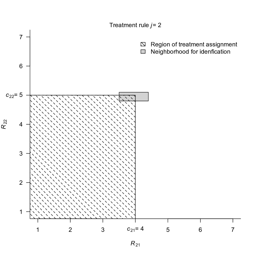
Now, let $Y_{i}(1)$ and $Y_{i}(0)$ denote the potential outcomes of unit $i$ under treatment and control, respectively. This notation implicitly makes the Stable Unit Treatment Value Assumption (SUTVA; Rubin 1980), which states that the treatment assignment of one unit does not affect the potential outcomes of other units and that there are no hidden versions of the treatment beyond those encoded by the treatment assignment indicator. In our framework, SUTVA is required only for units in a neighborhood of the cutoffs. Finally, let $\boldsymbol{X}_{i}$ denote a vector of observed, pretreatment covariates other than the running variables.

3.2 Estimand

We wish to estimate the average treatment effect in a neighborhood of the cutoffs where the treatment assignment is unconfounded given the observed covariates (which we term the “discontinuity neighborhood”). We call this estimand the Neighborhood Average Treatment Effect (NATE) and define it as

$$\tau_{\rm{NATE}}=\mathbb{E}\big{\{}Y_{i}(1)-Y_{i}(0)\ \big{|}\ N_{i}=1\big{\}}=\mathbb{E}\bigl{[}\mathbb{E}\bigl{\{}Y_{i}(1)-Y_{i}(0)\ \big{|}\ \boldsymbol{X}_{i},\ N_{i}=1\bigl{\}}\big{|}N_{i}=1\bigl{]}.$$ (5)

In our case study, this is the average effect of grade retention on criminal and educational outcomes for similar students in the discontinuity neighborhood. Possibly, this average effect varies across treatment rules; e.g., the effect of repeating under rule 1 differs from rule 2. Likewise, the effect of repeating could vary across running variables within the same rule; e.g., the effect of repeating differs across school subjects (see Wong et al. 2013, and Choi and Lee 2018, for a related discussion and methods). Furthermore, the effects could be modified by covariates; e.g., the effect of repeating is different for boys and girls. In brief, within the discontinuity neighborhood the effects can be heterogeneous on the treatment rules, running variables, and the covariates. From (5), we note that $\mathbb{E}\bigl{\{}Y_{i}(1)-Y_{i}(0)\ \big{|}\ \boldsymbol{X}_{i},\ N_{i}=1\bigl{\}}$ is the Conditional Average Treatment Effect (CATE) in the discontinuity neighborhood (see Chapter 12 of Imbens and Rubin 2015, for a discussion of the CATE). Under the following assumptions, all these heterogenous effects can be analyzed as in observational studies with strongly ignorable treatment assignment, albeit confined to a discontinuity neighborhood.

3.3 Assumptions

3.3.1 Assumptions for identification

In this section we state the assumptions needed to identify the NATE.

Assumption 1 (local strong ignorability of treatment assignment via the running variables).

Assumption 1a

$$\{\boldsymbol{R}_{ij}:j=1,...,\mathrm{J}\}\mathchoice{\mathrel{\hbox to0.0pt{$\displaystyle\perp$\hss}\mkern 2.0mu{\displaystyle\perp}}}{\mathrel{\hbox to0.0pt{$\textstyle\perp$\hss}\mkern 2.0mu{\textstyle\perp}}}{\mathrel{\hbox to0.0pt{$\scriptstyle\perp$\hss}\mkern 2.0mu{\scriptstyle\perp}}}{\mathrel{\hbox to0.0pt{$\scriptscriptstyle\perp$\hss}\mkern 2.0mu{\scriptscriptstyle\perp}}}\{Y_{i}(1),Y_{i}(0)\}\,|\,\boldsymbol{X}_{i},N_{i}=1$$

Assumption 1b

$$0<\mathrm{Pr}(Z_{i}=1\ |\ \boldsymbol{X}_{i},N_{i}=1)<1$$

∎

Assumption 1 has two components: local unconfoundedness and local positivity of treatment assignment via the running variables. Assumption 1a states that, in a neighborhood of the cutoffs, the running variables — and, therefore, the assignment to treatments — are independent of the potential outcomes given the observed covariates. Assumption 1b states that in this discontinuity neighborhood every unit has a positive probability of receiving any version of the treatment given the observed covariates. See Cattaneo et al. (2015) and Li et al. (2015) for a discussion of these assumptions under the local randomization framework with simple treatment rules.

Under Assumptions 1a and 1b, we can non-parametrically identify $\tau_{\rm{NATE}}$ in (5) using the following identity:

$$\mathbb{E}\big{\{}Y_{i}(1)-Y_{i}(0)\big{|}N_{i}=1\big{\}}=\mathbb{E}\big{\{} \mathbb{E}\big{(}Y_{i}\ \big{|}\ Z_{i}=1,\ \boldsymbol{X}_{i},\ N_{i}=1\big{)}$$

$$-\mathbb{E}\big{(}Y_{i}\ \big{|}Z_{i}=0,\ \boldsymbol{X}_{i},\ N_{i}=1\big{)}\big{|}N_{i}=1\big{\}}.$$

In other words, under Assumptions 1a and 1b, a discontinuity design can be analyzed as an observational study under strong ignorability (Rosenbaum and Rubin 1983), but confined to a discontinuity neighborhood. As we discuss below, this “local strong ignorability” assumption facilitates a series of tasks that are typically precluded in discontinuity designs under usual assumptions such as handling multiple treatment rules and generalizing effect estimates. It also suggests using other methods for outcome analyses normally used in observational studies such as those described in Section 4. For a more detailed discussion about the assumption of strong ignorability in observational studies, see, e.g., Chapter 12 of Imbens and Rubin (2015).

Assumptions 1a and 1b are different from the usual assumptions in the continuity-based and the local randomization frameworks. One could argue that the above assumptions are stronger than the typical ones in the continuity-based framework; however, the frameworks target different estimands (see, for instance, De la Cuesta and Imai 2016, and Mattei and Mealli 2016). In our framework the estimand is the Neighborhood Average Treatment Effect, whereas in the continuity-based framework the estimand is the average effect at the cutoff. In both cases, these are local estimands (as opposed to estimands for the general population), although the local randomization framework can facilitate the generalization of causal inferences to other populations (see Section 3.3.2). We can say that there is a trade-off between invoking different assumptions and identifying different estimands. While our framework builds on the local randomization framework, its assumptions are more plausible in practice than the ones in typical local randomization settings, because in many applications local independence conditional on covariates is a more realistic assumption than unconditional local independence. In our case study, even in the smallest possible discontinuity neighborhood there are imbalances in relevant covariates measuring the student’s ability. However, after adjusting for these and other educational and sociodemographic covariates, treatment assignment can be considered as-if randomized in a discontinuity neighborhood, because other covariates are balanced, but not across the entire range of the running variables. The validity of these assumptions is, of course, context-specific and must be carefully evaluated in the setting under study.

3.3.2 Assumptions for generalization

For generalization — that is, for identification and estimation of average treatment effects in target populations beyond the sample considered in the analysis — we consider two relevant cases. In both cases, selection into the sample is determined by observed covariates, in addition to the running variables. The key distinction is whether the target population has values of the running variables inside the neighborhood. The case where the target population has values of the running variables outside the neighborhood naturally involves stronger assumptions that, as we discuss below, contradict Assumptions 1a and 1b because they require treatment assignment to be strongly ignorable throughout the entire range of the running variables.

Let $\mathscr{P}$ be a target population and $\mathcal{S}$ be the sample of units from $\mathscr{P}$ selected into the neighborhood of the cutoffs where assumptions 1a and 1b are believed to hold. Write $S_{i}=1$ if unit $i$ is selected into the sample and $S_{i}=0$ otherwise. Here, we wish to identify and estimate the target average treatment effect (TATE; Kern et al. 2016)

$$\tau_{\textrm{TATE}}:=\mathbb{E}_{\mathscr{P}}\{Y_{i}(1)-Y_{i}(0)\},$$

that is, the average treatment effect in the target population $\mathscr{P}$.

$\bullet$ Case 1: $\mathscr{P}$ such that $N_{i}=1$ for all $i\in\mathscr{P}$

In this case, we assume the following two conditions hold.

Assumption 2 (strong ignorability of study selection in a neighborhood).

Assumption 2a

$$\{Y_{i}(1),Y_{i}(0)\}\mathchoice{\mathrel{\hbox to0.0pt{$\displaystyle\perp$\hss}\mkern 2.0mu{\displaystyle\perp}}}{\mathrel{\hbox to0.0pt{$\textstyle\perp$\hss}\mkern 2.0mu{\textstyle\perp}}}{\mathrel{\hbox to0.0pt{$\scriptstyle\perp$\hss}\mkern 2.0mu{\scriptstyle\perp}}}{\mathrel{\hbox to0.0pt{$\scriptscriptstyle\perp$\hss}\mkern 2.0mu{\scriptscriptstyle\perp}}}S_{i}\,|\,\boldsymbol{X}_{i},N_{i}=1$$

Assumption 2b

$$0<\Pr(S_{i}=1|\boldsymbol{X}_{i},N_{i}=1)<1$$

∎

Assumption 2a states that selection into the sample is independent of the potential outcomes given the observed covariates and that the running variables take values in the neighborhood of the cutoffs. Assumption 2b states that every unit in the target population $\mathscr{P}$ has a positive probability of selection into the sample given identical conditions on the observed covariates and running variables.

Under assumptions 1a, 1b, 2a, and 2b, we can identify $\tau_{\textrm{TATE}}$ from

$$\mathbb{E}_{\mathscr{P}}\big{\{}Y_{i}(z)\big{|}N_{i}=1\big{\}}=\mathbb{E}_{\mathscr{P}}\big{\{}\mathbb{E}\big{(}Y_{i}\big{|}S_{i}=1,\ Z_{i}=z,\ \boldsymbol{X}_{i},\ N_{i}=1\big{)}\big{|}\ N_{i}=1\big{\}},$$

for $z=0,1$.

$\bullet$ Case 2: $\mathscr{P}$ such that $N_{i}\neq 1$ for some $i\in\mathscr{P}$

In this case, we assume the following two conditions hold.

Assumption 3 (strong ignorability of study selection).

Assumption 3a

$$\{Y_{i}(1),Y_{i}(0)\}\mathchoice{\mathrel{\hbox to0.0pt{$\displaystyle\perp$\hss}\mkern 2.0mu{\displaystyle\perp}}}{\mathrel{\hbox to0.0pt{$\textstyle\perp$\hss}\mkern 2.0mu{\textstyle\perp}}}{\mathrel{\hbox to0.0pt{$\scriptstyle\perp$\hss}\mkern 2.0mu{\scriptstyle\perp}}}{\mathrel{\hbox to0.0pt{$\scriptscriptstyle\perp$\hss}\mkern 2.0mu{\scriptscriptstyle\perp}}}S_{i}\,|\,\boldsymbol{X}_{i}$$

Assumption 3b

$$0<\Pr(S_{i}=1|\boldsymbol{X}_{i})<1$$

∎

Assumptions 3a and 3b are stronger than Assumptions 2a and 2b. Under these assumptions, we need to modify assumptions 1a and 1b in order to identify $\tau_{\textrm{TATE}}$. In fact, under these assumptions we must have strong ignorability of treatment assignment via the running variables; that is, $\{\boldsymbol{R}_{ij}:j=1,...,\mathrm{J}\}\mathchoice{\mathrel{\hbox to0.0pt{$\displaystyle\perp$\hss}\mkern 2.0mu{\displaystyle\perp}}}{\mathrel{\hbox to0.0pt{$\textstyle\perp$\hss}\mkern 2.0mu{\textstyle\perp}}}{\mathrel{\hbox to0.0pt{$\scriptstyle\perp$\hss}\mkern 2.0mu{\scriptstyle\perp}}}{\mathrel{\hbox to0.0pt{$\scriptscriptstyle\perp$\hss}\mkern 2.0mu{\scriptscriptstyle\perp}}}\{Y_{i}(1),Y_{i}(0)\}\,|\,\boldsymbol{X}_{i}$ and $0<\mathrm{Pr}(Z_{i}=1|\boldsymbol{X}_{i})<1$. In other words, the assignment of the running variables must be strongly ignorable given the observed covariates throughout the entire range of the running variables. Clearly, these are strong assumptions that deviate from traditional discontinuity settings.

4 Estimation and inference

4.1 Matching approaches

Let $\mathcal{I}_{T}$ and $\mathcal{I}_{C}$ be the set of indices of the treated and control units in $\mathcal{S}$. Specifically, let $\mathcal{I}_{T}=\{i:\ Z_{i}=1\ \textrm{and}\ N_{i}=1\}$ and $\mathcal{I}_{C}=\{i:\ Z_{i}=0\ \textrm{and}\ N_{i}=1\}$. Following Zubizarreta et al. (2014), we may find the largest pair-matched sample $\boldsymbol{m}^{*}$ of treatment and control units that is balanced in a neighborhood of the cutoffs as

$$\arg\!\max_{\boldsymbol{m}}\bBigg@{2.25} \sum_{t\in\mathcal{I}_{T}}\sum_{c\in\mathcal{I}_{C}}m_{tc}:$$ (6)

$$\left|\sum_{t\in\mathcal{I}_{T}}\sum_{c\in\mathcal{I}_{C}}m_{tc}\{B_{q}(\boldsymbol{X}_{t})-\sum_{i\in\mathcal{P}}B_{q}(\boldsymbol{X}_{i})\}\right|\leq\delta_{q}\sum_{t\in\mathcal{I}_{T}}\sum_{c\in\mathcal{I}_{C}}m_{tc},\>q=1,\ldots,\mathrm{Q};$$ (7)

$$\left|\sum_{t\in\mathcal{I}_{T}}\sum_{c\in\mathcal{I}_{C}}m_{tc}\{B_{q}(\boldsymbol{X}_{c})-\sum_{i\in\mathcal{P}}B_{q}(\boldsymbol{X}_{i})\}\right|\leq\delta_{q}\sum_{t\in\mathcal{I}_{T}}\sum_{c\in\mathcal{I}_{C}}m_{tc},\>q=1,\ldots,\mathrm{Q};$$ (8)

$$m_{tc}\in\{0,1\},t\in\mathcal{I}_{T},c\in\mathcal{I}_{C}\bBigg@{2.25}\}$$ (9)

where $m_{tc}$ are binary decision variables that determine whether treated unit $t$ is matched to control unit $c$; $B_{q}(\boldsymbol{X}_{t})$ are suitable transformations of the observed covariates that span a certain function space; and $\delta_{q}$ is a tolerance that restrains the imbalances in the functions $B_{q}(\cdot)$ of the covariates (see Wang and Zubizarreta 2020, for a tuning algorithm). Thus, the matching given by (6)-(9) is the maximal size pair-matching that approximately balances the transformations $B_{q}(\cdot)$ of the covariates relative to the target population $\mathscr{P}$. Following Zubizarreta et al. (2014), we can re-match the matching $\boldsymbol{m}^{*}$ in order to minimize the total sum of covariate distances between matched units, while preserving aggregate covariate balance. After matching, we can do inference using randomization techniques as in Rosenbaum (2002b) or the large sample approximations in Abadie and Imbens (2006).

4.2 Weighting approaches

The previous matching approach (6)-(9) can be seen as a form of weighting where the weights are binary (or a constant fraction) that encode an assignment between matched units. An alternative is to relax this matching problem into a weighting problem as follows,

$$\mathop{\mathrm{argmin}}_{\boldsymbol{w}}\bBigg@{2.25}\{ \sum_{i\in\mathcal{I}_{C}}\left(w_{i}-\bar{w}\right)^{2}:$$ (10)

$$\left|\sum_{i\in\mathcal{I}_{C}}w_{i}Z_{i}B_{q}(\boldsymbol{X}_{i})-\frac{1}{|\mathcal{I}_{T}|}\sum_{i\in\mathcal{I}_{T}}B_{q}(\boldsymbol{X}_{i})\right|\leq\delta_{q},\>q=1,\ldots,\mathrm{Q};$$ (11)

$$\sum_{i\in\mathcal{I}_{C}}w_{i}=1,w_{i}\geq 0,i\in\mathcal{I}_{C}\bBigg@{2.25}\}.$$ (12)

These are the weights $\boldsymbol{w}^{*}$ of minimum variance that approximately balance the covariates. The asymptotic properties and inferential methods with balancing weights are discussed in Zhao (2019) and Wang and Zubizarreta (2020).

4.3 Regression-assisted approaches

The above matching and weighting approaches can be complemented with additional regression adjustments. Here we present two regression-assisted approaches that follow the above matching and weighting approaches.

For matching, following Rubin (1979), we may use a Regression Assisted Matching (RAM) estimator of the form

$$\hat{\tau}_{\textrm{RAM}}=(\bar{y}_{T\cdot}-\bar{y}_{C\cdot})-(\bar{\boldsymbol{x}}_{T\cdot}-\bar{\boldsymbol{x}}_{C\cdot})\hat{\boldsymbol{\beta}}$$ (13)

where $\bar{y}_{T\cdot}$ and $\bar{y}_{C\cdot}$ are the means of $Y$ in the matched treated and control samples, and analogously, $\boldsymbol{x}_{T\cdot}$ and $\bar{\boldsymbol{x}}_{C\cdot}$ are the means of $\boldsymbol{x}$. The vector $\hat{\boldsymbol{\beta}}$ comprises the estimated linear regression coefficients of the matched-pair differences in outcomes on the matched-pair differences in covariates.

For weighting, following Athey et al. (2018), we may use a Regression Assisted Weighting (RAW) estimator of the form

$$\hat{\tau}_{\textrm{RAW}}=\bar{\boldsymbol{x}}_{T\cdot}\hat{\boldsymbol{\beta}}_{T}-\left\{\bar{\boldsymbol{x}}_{T\cdot}\hat{\boldsymbol{\beta}}_{C}+\sum_{i\in\mathcal{I}_{C}}w_{i}(y_{i}-\boldsymbol{x}_{i}\hat{\boldsymbol{\beta}}_{C})\right\}$$ (14)

where $\hat{\boldsymbol{\beta}}_{T}$ and $\hat{\boldsymbol{\beta}}_{C}$ are the estimated regression coefficients for the treated and control samples, respectively. For inference, given the selected neighborhood, we may use the methods in Athey et al. (2018) and Hirshberg and Wager (2018). See Robins et al. (1994) and Abadie and Imbens (2011) for related estimators.

5 Selection of the neighborhood

A central question in practice is how to select a neighborhood for analysis; that is, the region around the cutoffs where the identification assumptions are likely to hold. Assumptions 1a and 1b require that at least one neighborhood exists. In order to maximize the precision of the study, we will find the largest neighborhood where the assumptions are plausible.

Assumption 1a is not directly testable from the observed data. However, there are implications of this assumption that can be tested. In this paper, we present two sets of methods for testing such implications and selecting the neighborhood. The first set of methods is design-based in the sense that they do not use outcome information. The second set of methods is semi-design-based in that they use outcome information, but in a planning sample, separate from the sample used for the actual outcome analyses. We present this second set of methods in Appendix G in the Supplementary Materials.

One implication of 1a is balance on the potential outcomes and any other variable measured before treatment assignment, given the observed covariates $\boldsymbol{X}$. Let $\boldsymbol{X}^{\textrm{test}}$ denote such other variables. These variables can be secondary covariates, lagged outcomes, or lagged running variables, and are different from the observed covariates $\boldsymbol{X}$ required in Assumption 1a. Conditional on $\boldsymbol{X}$, Assumption 1a implies that $\boldsymbol{X}^{\textrm{test}}$ is balanced across treatment groups in terms of its joint distribution, and therefore, in terms of its moments.

To assess Assumption 1a, we may test for joint, multivariate covariate balance on $\boldsymbol{X}^{\textrm{test}}$ conditional on $\boldsymbol{X}$. For instance, we may use the cross-match test to compare multivariate distributions (Rosenbaum 2005; Heller et al. 2010). We will consider the assumption of local unconfoundedness to be plausible if we fail to reject the null hypothesis that $\boldsymbol{X}^{\textrm{test}}$ has the same multivariate distribution across treatment groups after adjusting for $\boldsymbol{X}$. In addition, we may test the validity of Assumption 1a by checking the following balance conditions

$$\mathbb{E}\bigl{[}\mathbb{E}\bigl{\{}h(\boldsymbol{X}_{i}^{\textrm{test}})\ \big{|}Z_{i}=1,\ \boldsymbol{X}_{i},\ N_{i}=1\bigl{\}}-\mathbb{E}\bigl{\{}h(\boldsymbol{X}_{i}^{\textrm{test}})\ \big{|}Z_{i}=0,\ \boldsymbol{X}_{i},\ N_{i}=1\bigl{\}}\big{|}N_{i}=1\bigl{]}=0,$$ (15)

for any function $h(\cdot)$. For instance, (15) can be tested after matching using randomization techniques. The idea is to find the largest neighborhood of the cutoffs such that $\boldsymbol{X}^{\textrm{test}}$ is balanced after adjusting for $\boldsymbol{X}$ by matching. In practice, a conservative way to select this neighborhood is to implement different tests for univariate and multivariate covariate balance and select the largest neighborhood where we fail to reject the null hypothesis of covariate balance for any of the tests. See Appendix G for details.

6 Impact of grade retention on later life outcomes

6.1 Finding a neighborhood for analysis

To find the discontinuity neighborhood, we follow the design-based approach described in Section 5, where secondary covariates are available. Here, $\boldsymbol{X}^{\textrm{test}}$ is a three-dimensional vector that includes both parents’ education (measured in years of schooling), and the household per capita income (measured in pesos). $\boldsymbol{X}$ includes the student’s school attended and grade level in 2007, gender, birth year and month, number of times of previous grade retention, and standardized test scores in language and math.

Under Assumption 1a, $\boldsymbol{X}^{\textrm{test}}$ should be balanced across treatment groups in the discontinuity neighborhood ($N=1$), after conditioning on $\boldsymbol{X}$. We can check the following balance conditions

$$\mathbb{E}(\boldsymbol{X}_{i}^{\textrm{test}}\ |\ Z_{i}=1,\ \boldsymbol{X}_{i},\ N_{i}=1)=\mathbb{E}(\boldsymbol{X}_{i}^{\textrm{test}}\ |Z_{i}=0,\ \boldsymbol{X}_{i},\ N_{i}=1).$$ (16)

We use matching to adjust for the observed covariates and select the largest neighborhood that satisfies these conditions. In the spirit of Cattaneo et al. (2015), we implement a sequence of balance tests on $\boldsymbol{X}^{\textrm{test}}$ conditioning on $\boldsymbol{X}$ for a sequence of expanding neighborhoods and select the largest one where we fail to reject the above balance tests. We take the following steps in order to select a neighborhood for analysis.

1. Start with a small neighborhood around the cutoffs.

2. Find the largest matched sample in the neighborhood that balances the covariates $\boldsymbol{X}$.

3. Test that $\boldsymbol{X}^{\textrm{test}}$ has the same distribution across treatment groups using the cross-match test for multivariate balance and the permutational t-test for mean balance.

   1. If the minimum $p$-value is less than the critical value $p^{*}$, then repeat steps 1 to 3 starting with a smaller neighborhood.

   2. If the minimum $p$-value is greater than or equal to $p^{*}$, then expand the neighborhood and repeat steps 2 and 3 until the new minimum $p$-value is smaller than $p^{*}$.

4. Retain the largest neighborhood with a minimum $p$-value greater than or equal to $p^{*}$.

In our case study, we set $p^{*}$ to 0.1 (Cattaneo et al. 2015). As $p^{*}$ increases, the balance criteria becomes more stringent, and the resulting neighborhood is smaller; we set $p^{*}$ to 0.1 because it is is more conservative than setting it to 0.05. In step 2 we match students exactly on age (in months), gender, school, school grade, and past grade retention (number of times). In addition, we match for mean balance for the standardized test scores in language and mathematics. More specifically, we use cardinality matching (Zubizarreta et al. 2014) to find the largest pair-matched sample that is balanced according to these two exact matching and mean balance requirements. See Appendix A for a summary of covariate balance before and after matching.

Table 1 summarizes the process of selecting a neighborhood in our case study. In the first row of the table, we start with a neighborhood defined by $\underline{\delta}_{qr}=\overline{\delta}_{qr}=$ 0.1 for all the cutoffs $qr$ (0.1 is the minimum increment of school grades in Chile). This results in a matched sample of 243 pairs comprising 486 students. For this matched sample, we fail to reject the null hypothesis of no differences in secondary covariates (the minimum $p$-value is 0.33); therefore we expand the neighborhood as noted by the second line of the table. After expanding the neighborhood each time by 0.1 for $R_{11}$ and $R_{21}$ symmetrically (see Appendix G for details), we obtain a matched sample of 1,141 pairs comprising 2,282 students, with a neighborhood of rule 1 given by [3.5, 4.4]$\times$ [4.3, 4.6] and a neighborhood of rule 2 given by [3.5, 4.4] $\times$ [4.8, 5.1]. For the subsequent larger neighborhood, we reject the null hypothesis of balance on secondary covariates (the minimum $p$-value is 0.03). In our notation, the selected neighborhood of rule 1 is $[c_{11}-\underline{\delta}_{11},c_{11}+\overline{\delta}_{11}]\times[c_{12}-\underline{\delta}_{12},c_{12}+\overline{\delta}_{12}]$, and the corresponding neighborhood of rule 2 is $[c_{21}-\underline{\delta}_{21},c_{21}+\overline{\delta}_{21}]\times[c_{22}-\underline{\delta}_{22},c_{22}+\overline{\delta}_{22}]$, where $c_{11}=$3.9 and $c_{12}=$4.4 are the cutoff values of $R_{11}$ and $R_{12}$ under the rule 1, $c_{21}=$3.9 and $c_{21}=$4.9 are the cutoff values of $R_{21}$ and $R_{22}$ under the rule 2, with $\underline{\delta}_{11}=$0.4, $\overline{\delta}_{11}=$0.5, $\underline{\delta}_{12}=$0.1, $\overline{\delta}_{12}=$0.2, $\underline{\delta}_{21}=$0.4, $\overline{\delta}_{21}=$0.5, $\underline{\delta}_{22}=$0.1, and $\overline{\delta}_{22}=$0.2.

Table 1: Selection of a neighborhood for analysis

[t] Neighborhood Matched sample size $p$-value for the $p$-value for no effect Plausibility of Rule 1 Rule 2 Treated Control cross-match test on secondary covariates Assumption 1a $\text{[3.8, 4.1]}\times\text{[4.3, 4.6]}$ $\text{[3.8, 4.1]}\times\text{[4.8, 5.1]}$ 243 243 1.00 0.33 ✓ $\text{[3.7, 4.2]}\times\text{[4.3, 4.6]}$ $\text{[3.7, 4.2]}\times\text{[4.8, 5.1]}$ 524 524 1.00 0.87 ✓ $\text{[3.6, 4.3]}\times\text{[4.3, 4.6]}$ $\text{[3.6, 4.3]}\times\text{[4.8, 5.1]}$ 841 841 1.00 0.81 ✓ $\text{[3.5, 4.4]}\times\text{[4.3, 4.6]}$ $\text{[3.5, 4.4]}\times\text{[4.8, 5.1]}$ 1,141 1,141 1.00 0.16 ✓ $\text{[3.4, 4.5]}\times\text{[4.3, 4.6]}$ $\text{[3.4, 4.5]}\times\text{[4.8, 5.1]}$ 1,359 1,359 1.00 0.03 ✗ $\text{[3.3, 4.6]}\times\text{[4.3, 4.6]}$ $\text{[3.3, 4.6]}\times\text{[4.8, 5.1]}$ 1,578 1,578 1.00 0.01 ✗ Notes: the third to last column reports the $p$-value for the Cross-match Test for comparing two multivariate distributions, while the the second to last column reports the minimum $p$-value for the permutational $t$-test for matched pairs of differences on secondary covariates.

Because it does not require outcome information, this procedure for selecting the neighborhood is part of the design (as opposed to the analysis) stage of the study (Rubin 2008). As such, it can help investigators preserve the objectivity of the study and maintain the validity of its statistical tests. In this procedure, the choice of the covariates in $\boldsymbol{X}$ and $\boldsymbol{X}^{\textrm{test}}$ requires careful consideration of the treatment assignment mechanism in the problem at hand. In our study, the assignment mechanism can vary across schools and grades, hence we matched exactly for both of these covariates in $\boldsymbol{X}$. Conditional on these covariates, around a neighborhood of the cutoffs, the student’s educational readiness can play an important role in the assignment, hence we further adjusted for all the available standardized test scores.

Given all these covariates in $\boldsymbol{X}$, we have applied the ideas in Imbens and Rubin (2015, Chapter 21) for assessing unconfoundedness. Ideally, $\boldsymbol{X}^{\textrm{test}}$ will include variables known not to be affected by the treatment given the covariates in $\boldsymbol{X}$. These can be proxy or pseudo-outcomes, such as lagged outcomes measured before treatment. In our data set, we do not have lagged measures of all the study outcomes, but a proxy for them are the measures of social capital corresponding to the mother and father’s education, and the household per capita income. Here, the decision of which variables to include in $\boldsymbol{X}^{\textrm{test}}$ relies on substantive knowledge about the research question; however, one could consider more data-driven approaches that learn the covariates in $\boldsymbol{X}$ and $\boldsymbol{X}^{\textrm{test}}$ from the data itself. These approaches, nonetheless, should ponder the importance of separating the design and analysis stages of the study and preserving the validity of the statistical tests if they use the outcomes.

6.2 Three analyses

Having found the neighborhood, we proceed to estimate the effect of grade retention on subsequent school grades, repeating another grade, dropping out of school, or committing a juvenile crime. We consider three different analyses: one exploratory, where we visualize the impact of grade retention on subsequent grades across time; one based on randomization inference, where we perform a sensitivity analysis on an equivalence test; and one that combines approximately balancing weights and regularized regression. These analyses have contrasting strengths and can be complementary in practice.

6.2.1 Visualizing patterns of effects

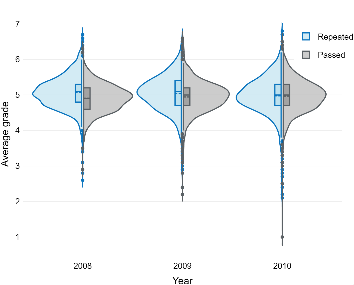
Figure 5: Average school grades of the matched students in the selected neighborhood. Here, we compare grades for the matched treated and control students from the same grade, for the first time they were taught that material.

In Figure 5, we plot the average school grades of the matched students within the selected neighborhood in years 2008-2011; that is, one, two, three, and four years after repeating or passing in 2007. In blue, we display the boxplots and densities of the average grades of the students who repeated, and in gray, of the students who passed. In 2008 (that is, in the year immediately after repeating or passing), the students who repeated had higher average grades than the matched students who passed. The difference is approximately 0.2 points (see Section 6.2.3 for point estimates and confidence intervals). However, this difference is progressively reduced in the three following years, declining to an average difference of 0.05 points in 2011. Interestingly, in 2011 the difference of the modes of the distributions of grades appears to be reverted, suggesting that after four years following repeating or passing, there are more students with lower grades after repeating than after passing, nonetheless the opposite happens in 2008. Between 2008 and 2011 the dispersion of the matched pair differences in outcomes increases from 0.56 to 0.75, suggesting that heterogeneity in treatment effects is increasing with time.

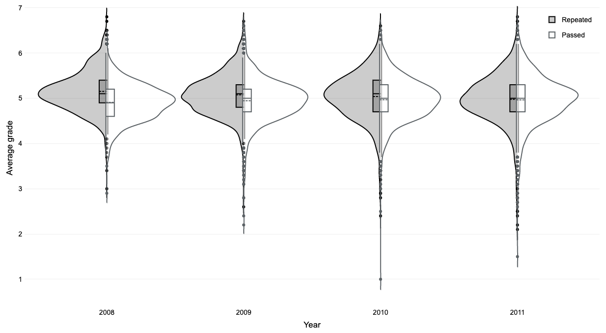
Figure 2: Average school grades of the matched students in the selected neighborhood.

6.2.2 Estimating effects using randomization tests

Here we estimate the effects (risk differences) of grade retention on repeating another grade, dropping out of school, and committing a juvenile crime. We use the methods in Rosenbaum (2002a) and Zubizarreta et al. (2013).

We test Fisher’s null hypothesis of no treatment effects using McNemar’s test statistic. In our example, this test statistic corresponds to the number of discordant pairs where the student that was retained subsequently repeated another grade, dropped out of school, or committed a juvenile crime. Figure 3 presents the point estimates and confidence intervals of the NATE on these three outcome variables. The point estimate of the effect of grade retention on juvenile crime is $\widehat{\tau}_{\rm{NATE}}^{\rm{crime}}$ = 0.006 ($p$-value = 0.229). In fact, among the 1,141 matched pairs, there are 117 discordant pairs in which only one student committed a crime. Of these, there are 62 pairs in which the student that repeated committed a crime (see Appendix C for details). Thus, in the absence of hidden bias, there is no evidence that grade retention causes juvenile crime. Similarly, the estimated effect of grade retention on dropping out of school is also very small ($\widehat{\tau}_{\rm{NATE}}^{\rm{drop}}$ = 0.002) and not statistically significant ($p$-value = 0.379). However, the estimated effect of grade retention on repeating another grade is $\widehat{\tau}_{\rm{NATE}}^{\rm{ret}}$ = -0.104. Here, there are 563 discordant pairs, and out of these, there are 222 pairs in which the student who was retained in 2007 did not repeat another grade in the future, yielding a one-sided $p$-value smaller than 0.001 (see Appendix C). Thus, in the absence of hidden bias, there is significant evidence that current grade retention causes a reduction in future grade retention. In Appendix H, we analyze the stability of these results to varying the neighborhood size, finding that they are generally robust to modifying the neighborhood for the lowest and second lowest grades, but somewhat sensitive to modifying the neighborhood for the average grade, emphasizing the importance of the selection of the neighborhood. In Appendix F, we provide guidance for generalizing these results.

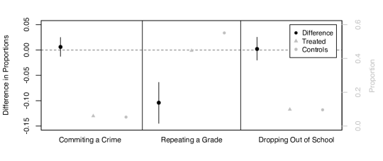
Figure 3: Estimates for the Neighborhood Average Treatment Effect

We also study how these effects vary by gender. This is straightforward because we matched exactly by that covariate. The results are reported in Tables 4 and 5 in Appendix C, and suggest that the effect of grade retention is not modified by gender. Under Assumptions 1a and 1b it is possible to study treatment effect heterogeneity in the discontinuity neighborhood using other regression approaches rather than matching.

In the absence of hidden bias, we have found evidence that grade retention does not cause dropping out of school or committing a juvenile crime. However, bias from a hidden covariate can give the impression that a treatment effect does not exist when in fact there is one. How much bias from a hidden covariate would need to be present to mask an actual treatment effect? We address this question with a sensitivity analysis on a near equivalence test (Rosenbaum and Silber 2009, Zubizarreta et al. 2013). Our results reveal that two students matched on their observed covariates could differ in their odds of repeating the grade in 2007 by almost 12% and 46% before masking small and moderate effects previously documented in the literature on juvenile crime. Analogously, two students matched for their covariates could differ in their odds of repeating by 16% and 33% before masking small and moderate effects on dropping out of school. See Appendices D and E for details.

6.2.3 Estimating effects using balancing weights and regularized regression

We use the regression assisted weighting estimator (14) to estimate the effect of grade retention on average school grades in subsequent school grades. More specifically, we use the method by Athey et al. (2018) which combines approximately balancing weights and regularized linear regression. We find that one year after retention, the average school grades of students who repeated is 0.19 points higher than the one of students that passed (95% confidence interval, [0.16, 0.21]; the standard deviation of average school grades this year was 0.46 points). Four years after retention, this effect is considerably reduced, and students who repeated have on average 0.05 points higher than students who passed (95% confidence interval, [0.01, 0.08]; the standard deviation of average school grades in that year was 0.63 points).

In summary, our results suggest that grade retention has a positive effect in the short run on future school grades, but that this effect dissipates over time — all this, among students who are comparable in terms of observed covariates and that barely pass or repeat the academic year. A number of mechanisms can explain this result. One of them is that retained students know the material better and are more mature. This is consistent with our other result that students who barely pass tend to repeat more in the future. It is also possible that school grades measure the students’ true ability with error, so that in the neighborhood below the cutoff, we have more students who suffered a negative transitory shock, while above the cutoff we have more students who suffered a positive transitory shock. In that case, it is possible that students that barely repeat are more likely to improve next year, and vice-versa, even if retention has no effect. Although it merits further investigation, this explanation may be limited as we adjust for educational and socioeconomic variables in the four years preceding the intervention of grade retention. This and other possible causal mechanisms that may explain our findings deserve closer examination. Finally, we estimate an almost null effect of grade retention on juvenile crime, with these results being insensitive to small and moderate hidden biases.

7 Further extensions

The proposed framework can also accommodate intermediate outcomes (i.e., principal stratification analyses). For example, it can be extended to instrumental variable (IV) analyses with noncompliance (Angrist et al. 1996), yet within a neighborhood of the cutoffs of the running variables. As mentioned, in discontinuity designs the IV approach to noncompliance is known as the fuzzy design, whereas the case with full compliance is known as the sharp design (Hahn et al. 2001). In a complex fuzzy discontinuity design (that is, when the treatment assignment is determined by multiple rules that possibly lead to the same treatment, but there is noncompliance), we can nonparametrically identify the average treatment effect for the compliers in the discontinuity neighborhood under two assumptions beyond assumptions 1a and 1b. Specifically, under the assumptions of local strong ignorability of treatment assignment (1a and 1b), local monotonicity (i.e., that the treatment assignment has a non-negative effect on the treatment exposure for all the units in a neighborhood of the cutoffs), and the local exclusion restriction (i.e., that the treatment assignment affects the outcome only through the treatment exposure for all the units the neighborhood), the average treatment effect for the compliers in the discontinuity neighborhood can be identify following the same arguments as those in the IV approach to noncompliance in randomized experiments (Imbens and Rubin 2015, chapters 23 and 24), but restricting the analysis to a neighborhood of the cutoffs.

8 Concluding remarks

Since their introduction in 1960 by Thistlethwaite and Campbell, regression discontinuity designs have proven to be a powerful method for drawing causal inferences in observational studies. However, they have often been confined to settings where treatment assignment is determined by simple rules. Although regression discontinuity designs under the continuity-based framework have been extended to separately incorporate multiple running variables or multiple cutoffs, to our knowledge they do not comprehend more complex treatment rules, such as those found in our case study. In this paper we have conceptualized a complex discontinuity design as a local randomized experiment conditional on covariates; or more specifically, as an observational study with strongly ignorable treatment assignment given covariates in a neighborhood of the cutoffs. In our case study, we found that grade retention in Chile has a negative impact on future grade retention, but is not associated with dropping out of school or committing a juvenile crime. As discussed, this framework can facilitate the generalization and transportation of causal inferences in discontinuity designs. Under this framework, it is straightforward to take advantage of methods not normally used in traditional regression discontinuity designs, such as simple graphical displays of outcomes as in clinical trials, and potentially statistical machine learning methods to estimate heterogeneous effects. Here, we have used matching to adjust for covariates and select the neighborhood, but under the assumptions of local strong ignorability other methods can be used. Future work can study the properties of regression assisted estimators in discontinuity designs and extend this framework to principal stratification analyses (see Li et al. 2015). In observational studies, discontinuities in treatment assignment rules offer a keyhole through which to see causality. Motivated by the problem of estimating the impact of grade retention on later life outcomes, in this paper we have proposed a framework and methods to leverage them with complex treatment rules.

Online supplementary materials

The following materials are organized as follows. Appendix A describes covariate balance before and after matching. Appendix B displays the outcomes after matching for students in the same grade. Appendix C includes additional explanations and results on the outcome analyses. Appendices D and E expand on the sensitivity analyses. Appendix F discusses generalization. Appendix G explains how to implement the design-based approach for selecting a neighborhood, presents a separate semi-design-based approach, and provides some practical considerations. Appendix H evaluates the stability of the results to varying the neighborhood size. Appendix I analyzes covariate balance under the continuity-based framework.

Appendix A: Covariate balance

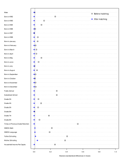
Figure 4: Standardized differences in means before and after matching inside the neighborhood $[3.5,4.4]\times[4.3,4.6]$ for rule 1 and $[3.5,4.4]\times[4.8,5.1]$ for rule 2.

Notes: inside the neighborhood, we match exactly on gender, year and month of birth, school and grade attended in 2007, and times of past grade retention. In addition, we match with mean balance on the SIMCE scores in language and mathematics. As a result, the mother and father’s schooling and the household income are also balanced.

Appendix B: Patterns of effects

Appendix C: Outcome analyses

We have $I=1,141$ matched pairs. In each pair $i\in\{1,2,\ldots,I\}$, one student $j\in\{1,2\}$ repeated the grade and the other passed. Following Rosenbaum (2002b), let $Z_{ij}=1$ if student $j$ in matched pair $i$ repeats and $Z_{ij}=0$ otherwise, so $Z_{i1}+Z_{i2}=1$ for all $i\in\{1,2,\ldots,I\}$. Student $j$ in pair $i$ exhibits potential outcome $Y_{ij}(1)$ if $Z_{ij}=1$, and potential outcome $Y_{ij}(0)$ if $Z_{ij}=0$. In the set $\mathcal{Z}$, we collect the $2^{I}$ possible treatment assignments, $\boldsymbol{Z}=(Z_{11},Z_{12},\ldots,Z_{I1},Z_{I2})^{\top}$. Under paired randomization, $\mathrm{Pr}\{Z_{ij}=1|Y_{ij}(1),Y_{ij}(0),u_{ij},\boldsymbol{X}_{ij},N_{ij}=1,\mathcal{Z}\}=1/2$, where $u_{ij}$ is an unobserved covariate. Let $\boldsymbol{Y}=(Y_{11},Y_{12},\ldots,Y_{I1},Y_{I2})^{\top}$ denote the vector of the observed outcomes for the $2I$ students and let $\boldsymbol{Y}(0)=(Y_{11}(0),Y_{12}(0),\ldots,Y_{I1}(0),Y_{I2}(0))^{\top}$ stand for the vector of potential outcomes under control for the $2I$ students. If $t(\boldsymbol{Z},\boldsymbol{Y})$ is a test statistic, then in a paired randomized experiment under Fisher’s null hypothesis of no treatment effect, the distribution of $t(\boldsymbol{Z},\boldsymbol{Y})$ is the permutation distribution

$$\mathrm{Pr}(t(\boldsymbol{Z},\boldsymbol{Y})>k|Y_{ij}(1),Y_{ij}(0),u_{ij},\boldsymbol{X}_{ij},N_{ij}=1,\mathcal{Z})=\frac{|\{\boldsymbol{Z}\in\mathcal{Z}:t(\boldsymbol{Z},\boldsymbol{Y}(0))>k\}|}{2^{I}}.$$ (25)

In our running example, the three outcomes of interest are binary. The first outcome takes the value 1 if the student committed a crime after 2007 and 0 otherwise; the second takes the value 1 if the student repeated a grade after 2007 and 0 otherwise; and the third takes the value 1 if the student dropped out of school after 2007 and 0 otherwise. To test $H_{0}$, we use McNemar’s test statistic: $t(\boldsymbol{Z},\boldsymbol{Y})=\sum_{i=1}^{I}\sum_{j=1}^{2}Z_{ij}Y_{ij}$, i.e., the number of responses equal to 1 among treated students. The results are as follows.

Table 2: Committing a juvenile crime in matched pairs. The table counts pairs, not students.

	Passed
Repeated	Juvenile crime = 0	Juvenile crime = 1
Juvenile crime = 0	1018	55
Juvenile crime = 1	62	6

Table 3: Dropping out of school in matched pairs. The table counts pairs, not students.

	Passed
Repeated	Dropped out = 0	Dropped out = 1
Dropped out = 0	945	84
Dropped out = 1	87	25

Table 4: Repeating another grade in matched pairs. The table counts pairs, not students.

	Passed
Repeated	Future retention = 0	Future retention = 1
Future retention = 0	290	341
Future retention = 1	222	288

Table 5: Estimates for the Neighborhood Average Treatment Effect, Boys (689 pairs)

[t] Outcome variable Matched sample mean $\widehat{\tau}_{\rm{NATE}}$ $H_{0}:\tau_{\rm{NATE}}=0$ Treated Control One-sided $p$-value Committing a crime 0.082 0.075 -0.007 <0.307 Repeating another grade 0.474 0.577 -0.103 <0.001 Dropping out of school 0.103 0.108 -0.005 <0.351

Table 6: Estimates for the Neighborhood Average Treatment Effect, Girls (452 pairs)

[t] Outcome variable Matched sample mean $\widehat{\tau}_{\rm{NATE}}$ $H_{0}:\tau_{\rm{NATE}}=0$ Treated Control One-sided $p$-value Committing a crime 0.024 0.020 -0.004 <0.381 Repeating another grade 0.404 0.511 -0.106 <0.001 Dropping out of school 0.901 0.075 -0.015 <0.185

Appendix D: Rosenbaum bounds to assess sensitivity to hidden bias

In the absence of hidden bias, there is strong evidence in our running example that current grade retention causes a reduction in future grade retention. How much hidden bias would need to be present to explain away this result? To answer this question, we implement the sensitivity analysis described in Rosenbaum (2002b, Chapter 4).

Let $\pi_{ij}$ denote the probability that student $j$ in pair $i$ repeats the grade (receives treatment). For each each pair $i$, two students match on their observed covariates, $\boldsymbol{X}_{ij}=\boldsymbol{X}_{ij^{{}^{\prime}}}$, but may differ on an unobserved covariate $u_{ij}\neq u_{ij^{{}^{\prime}}}$, such that $\pi_{ij}\neq\pi_{ij^{{}^{\prime}}}$. Suppose that the odds of repeating the grade differ at most by a factor $\Gamma\geq 1$

$$\frac{1}{\Gamma}\leq\frac{\pi_{ij}(1-\pi_{ij^{{}^{\prime}}})}{\pi_{ij^{{}^{\prime}}}(1-\pi_{ij})}\leq\Gamma$$

for each pair $i$. If $\Gamma=1$, then there is no hidden bias and the randomization distribution with $\pi_{ij}=\pi_{ij^{{}^{\prime}}}=1/2$ for McNemar’s test statistic is valid. If $\Gamma>1$, then there is hidden bias and there is a range of possible inferences for $\pi_{ij}\neq\pi_{ij^{{}^{\prime}}}$. These inferences are bounded by $\Gamma$ and $1/\Gamma$. For these two values, we obtain two extreme-case $p$-values. We look for the largest value of $\Gamma$ such that we reject the null hypothesis of no treatment effect.

In our running example, we are able to reject the null hypothesis that current grade retention does not causes future grade retention for $\Gamma=1.34$ (the upper bound of the $p$-value is 0.049) but not for $\Gamma>1.34$ (the upper bound of the $p$-value is greater than 0.05). In other words, two students matched for their observed covariates could differ in their odds of grade retention by 34% without materially altering the conclusions about the effect of current retention on future grade retention.

Appendix E: Sensitivity analysis on a near equivalence test

As discussed in Section 6.2.2, in the absence of hidden bias, we have found evidence that grade retention does not cause dropping out of school or committing a juvenile crime. However, bias from a hidden covariate can give the impression that a treatment effect does not exist when in fact there is one. How much bias from a hidden covariate would need to be present to mask an actual treatment effect? We answer this question by conducting a sensitivity analysis on a near-equivalence test. For details, see Rosenbaum and Silber (2009) and Zubizarreta et al. (2013).

Using the parameter $\Gamma$, we will test the null hypothesis that the effect of treatment is larger than a given effect size against the alternative hypothesis that it is lower. We take the effect size from previous studies in the literature. Our results will be insensitive to hidden bias if large values of $\Gamma$ are required to mask a given effect size. Before presenting the results of this sensitivity analysis, it is necessary to introduce the concept of an attributable effect (Rosenbaum 2002a).

For each of the two outcomes, committing a juvenile crime or dropping out of school, let $\bm{\delta}$ denote the $2I$-dimensional vector of treatment effects, with $\delta_{ij}=Y_{ij}(1)-Y_{ij}(0)$. Consider the hypothesis $H_{\bm{\delta_{0}}}:\bm{\delta}=\bm{\delta_{0}}$, where $\bm{\delta_{0}}$ is a $2I$-dimensional vector with values $\delta_{0ij}\in\{-1,0,1\}$. Clearly, not all hypotheses of this form are consistent with the data at hand, since $Y_{ij}-Z_{ij}\delta_{0ij}=Y_{ij}(0)$ and $Y_{ij}+(1-Z_{ij})\delta_{0ij}=Y_{ij}(1)$ must both be in $\{0,1\}$. Rosenbaum (2002a) summarizes hypotheses of the form $H_{\bm{\delta_{0}}}:\bm{\delta}=\bm{\delta_{0}}$ by introducing the attributable effect, which is defined as $\Delta=\sum_{i=1}^{I}\sum_{j=1}^{2}Z_{ij}\delta_{ij}$. In other words, the attributable effect is the number of treated students who experienced events caused by the treatment.

We assume that $Y_{ij}(1)\geq Y_{ij}(0)$ for each student $j$ in pair $i$; that is, that the exposure to treatment may cause the outcome in a student who would not otherwise experience it, but the treatment does not prevent the outcome in a student who would otherwise experience it. We consider the hypothesis $H_{\bm{\delta_{0}}}:\bm{\delta}=\bm{\delta_{0}}$, where $\delta_{0ij}\in\{0,1\}$. We can repeat this exercise reversing the roles of treatment and control. We again use McNemar’s test statistic. Under $H_{\bm{\delta_{0}}}:\bm{\delta}=\bm{\delta_{0}}$, $\Delta$ may be calculated using $\bm{\delta_{0}}$, $\Delta_{0}=\sum_{i=1}^{I}\sum_{j=1}^{2}Z_{ij}\delta_{0ij}$ and $t(\boldsymbol{Z},\boldsymbol{Y}(0))$ can be computed. A value of $\Delta_{0}$ is rejected if every hypothesis $H_{\bm{\delta_{0}}}:\bm{\delta}=\bm{\delta_{0}}$ with $\delta_{0ij}\in\{0,1\}$ that gives rise to this value of $\Delta_{0}$ is rejected. Given $\Delta_{0}$, among all the hypotheses $H_{\bm{\delta_{0}}}:\bm{\delta}=\bm{\delta_{0}}$ with $\delta_{0ij}\in\{0,1\}$ that give rise to this value of $\Delta_{0}$, there is one that is the most difficult to reject, such that if it is rejected then the associated value of $\Delta_{0}$ is rejected. rosenbaum2001effects proves that the hypothesis that is the most difficult to reject has $\sum_{j=1}^{2}Z_{ij}\delta_{ij}=1$ for as many pairs with $Y_{i1}+Y_{i2}=2$ as possible.

When conducting the test of equivalence on the matched pairs, we use two values for the attributable effect on juvenile crime ($\Delta^{crime}_{0}\in\{30,40\}$) and also two values for the attributable effect on dropping out of school ($\Delta^{drop}_{0}\in\{40,50\}$). For example, an attributable effect on juvenile crime of 40 is equivalent to saying that 40 juvenile crimes are attributed to grade retention. The order of magnitude of these attributable effects are taken from previous studies in the literature. Utilizing a standard fuzzy RDD, Erena et al. (2017) estimate the impact of grade retention on dropping out of school in the state of Louisiana, finding a point estimate of 4.8% (equivalent to 55 cases of dropping out of school attributed to grade retention in our context), whereas Díaz et al. (2021) estimate the effect of grade retention on juvenile crime in Chile, obtaining a point estimate of 4.3% (equivalent to 49 juvenile crimes attributed to grade retention in our application).

We are able to reject the null hypothesis that $H_{0}:\Delta^{crime}\geq 30$ for $\Gamma=1.12$ with an upper bound of the $p$-value of 0.049 (Table 7 presents the adjusted pairs), whereas we reject the null hypothesis that $H_{0}:\Delta^{crime}\geq 40$ for $\Gamma=1.46$ with an upper bound of the $p$-value of 0.047 (Table 8 presents the adjusted pairs). These results reveal that two students matched on the basis of their observed covariates could differ in their odds of repeating the grade in 2007 by almost 12% before masking an attributable effect on juvenile crime of 30, and by almost 46% before masking an attributable effect of 40. In the same manner, $H_{0}:\Delta^{drop}\geq 40$ is rejected for $\Gamma=1.16$ with the upper bound of the $p$-value of 0.047 (Table 9 presents the adjusted pairs), whereas $H_{0}:\Delta^{drop}\geq 50$ is also rejected for $\Gamma=1.33$ with the upper bound of the $p$-value of 0.045 (Table 10 presents the adjusted pairs). In words, these results suggest that two students matched for their observed covariates could differ in their odds of repeating the grade in 2007 by almost 16% before masking an attributable effect of 40 on dropping out of school, and by almost 33% before masking an attributable effect of 50.

Table 7: Juvenile crime indicators in matched pairs adjusted for the null hypothesis $H_{0}:\bm{\delta^{crime}}=\bm{\delta_{0}^{crime}}$ that attributes $\sum_{i=1}^{I}\sum_{j=1}^{2}Z_{ij}\delta_{ij}^{crime}=30$ juvenile crimes to grade retention. The table counts pairs, not students.

	Passed
Repeated	Juvenile crime = 0	Juvenile crime = 1
Juvenile crime = 0	1042	61
Juvenile crime = 1	38	0

Table 8: Juvenile crime indicators in matched pairs adjusted for the null hypothesis $H_{0}:\bm{\delta^{crime}}=\bm{\delta_{0}^{crime}}$ that attributes $\sum_{i=1}^{I}\sum_{j=1}^{2}Z_{ij}\delta_{ij}^{crime}=40$ juvenile crimes to grade retention. The table counts pairs, not students.

	Passed
Repeated	Juvenile crime = 0	Juvenile crime = 1
Juvenile crime = 0	1052	61
Juvenile crime = 1	28	0

Table 9: Dropping out of school indicators in matched pairs adjusted for the null hypothesis $H_{0}:\bm{\delta^{drop}}=\bm{\delta_{0}^{drop}}$ that attributes $\sum_{i=1}^{I}\sum_{j=1}^{2}Z_{ij}\delta_{ij}^{drop}=40$ cases of dropping out of school to grade retention. The table counts pairs, not students.

	Passed
Repeated	Dropped out = 0	Dropped out = 1
Dropped out = 0	960	109
Dropped out = 1	72	0

Table 10: Dropping out of school indicators in matched pairs adjusted for the null hypothesis $H_{0}:\bm{\delta^{drop}}=\bm{\delta_{0}^{drop}}$ that attributes $\sum_{i=1}^{I}\sum_{j=1}^{2}Z_{ij}\delta_{ij}^{drop}=50$ cases of dropping out of school to grade retention. The table counts pairs, not students.

	Passed
Repeated	Dropped out = 0	Dropped out = 1
Dropped out = 0	970	109
Dropped out = 1	62	0

Appendix F: Generalizing the results

Here we generalize our results to a target population. Under the Assumptions 1a, 1b, 2a, and 2b, we can estimate the average treatment effect on a target population with running variables in the neighborhood. We define the target population on the basis of household income. Among students with values of the running variables in the neighborhood previously determined, the target population consists of students in the poorest 50% of households.

Table 11: Description of the target population and the matched sample within the window $[3.5,4.4]\times[4.3,4.6]$ for rule 1 and $[3.5,4.4]\times[4.8,5.1]$ for rule 2.

[t] Covariate Full sample mean of the Matched sample mean poorest 50% of households Treated Control Male 0.60 0.60 0.60 Born in 1992 0.05 0.01 0.01 Born in 1993 0.14 0.12 0.12 Born in 1994 0.22 0.26 0.26 Born in 1995 0.18 0.24 0.24 Born in 1996 0.10 0.17 0.17 Born in 1997 0.07 0.11 0.11 Born in 1998 0.08 0.09 0.09 Born in January 0.09 0.10 0.10 Born in February 0.08 0.08 0.08 Born in March 0.08 0.09 0.09 Born in April 0.08 0.08 0.08 Born in May 0.09 0.06 0.06 Born in June 0.09 0.07 0.07 Born in July 0.08 0.08 0.08 Born in August 0.08 0.09 0.09 Born in September 0.08 0.08 0.08 Born in October 0.09 0.09 0.09 Born in November 0.09 0.09 0.09 Born in December 0.09 0.09 0.09 Public School 0.68 0.43 0.43 Subsidized School 0.32 0.57 0.57 3th grade 0.07 0.05 0.05 4th grade 0.08 0.08 0.08 5th grade 0.17 0.17 0.17 6th grade 0.31 0.21 0.21 7th grade 0.23 0.32 0.32 8th grade 0.13 0.17 0.17 Previous grade retention 0.39 0.09 0.09 SIMCE Math -0.53 -0.26 -0.25 SIMCE Language -0.51 -0.27 -0.26 Father schooling 9.27 11.37 11.42 Mother schooling 9.08 11.13 11.24 Household income per capita 40,720.06 92,373.58 92,297.38 Notes: in a neighborhood of the cutoffs, we do exact matching on school, grade attended in 2007, gender, birth month and year, and times of past grade retention, while mean balance matching on SIMCE’s score in math and language. The secondary covariates are father and mother schooling, and household income per capita.

Following Zubizarreta et al. (2018), we use cardinality matching to find the largest matched sample that is not only balanced across treatment groups, but is also balanced around the distribution of a target population of interest. Within the window previously determined, Table 11 compares the means of the treated and control students in the matched sample to the means of students in the poorest 50% of households, whereas Table 12 compares the means of the treated and control students in the representative matched sample to the means of students in the poorest 50% of households. To find the representative matched sample, we require that the absolute standardized differences in means between the matched treated students and all students in the target population, and between the matched control students and all students in the target population, are all smaller than 0.05.

Having found a representative matched sample of 283 pairs of students, we assume that treatment is as-if randomly assigned to students conditional on the matched pairs. Table 13 presents the results when generalizing the effect estimates to the population of the poorest 50% of students with grades in the selected neighborhood, while Tables 14, 15, and 16 detail the discordant pairs for committing a crime, dropping out of school, and repeating another grade, respectively. In the absence of hidden bias, there is no evidence that grade retention causes juvenile crime (the two-sided $p$-value is 0.359) nor dropping out of school ($p$-value = 0.464), whereas there is statistically significant evidence that grade retention reduces the probability of future grade retention ($p$-value = 0.049).

Table 12: Description of the target population and the representative matched sample within the window $[3.5,4.4]\times[4.3,4.6]$ for rule 1 and $[3.5,4.4]\times[4.8,5.1]$ for rule 2.

[t] Covariate Full sample mean of the Matched sample mean poorest 50% of households Treated Control Male 0.60 0.61 0.61 Born in 1992 0.05 0.04 0.04 Born in 1993 0.14 0.12 0.12 Born in 1994 0.22 0.20 0.20 Born in 1995 0.18 0.18 0.18 Born in 1996 0.10 0.09 0.09 Born in 1997 0.07 0.08 0.08 Born in 1998 0.08 0.10 0.10 Born in January 0.09 0.07 0.07 Born in February 0.08 0.07 0.07 Born in March 0.08 0.08 0.08 Born in April 0.08 0.09 0.09 Born in May 0.09 0.07 0.07 Born in June 0.09 0.07 0.07 Born in July 0.08 0.07 0.07 Born in August 0.08 0.08 0.08 Born in September 0.08 0.10 0.10 Born in October 0.09 0.10 0.10 Born in November 0.09 0.09 0.09 Born in December 0.09 0.09 0.09 Public School 0.68 0.66 0.66 Subsidized School 0.32 0.34 0.34 3th grade 0.07 0.07 0.07 4th grade 0.08 0.07 0.07 5th grade 0.17 0.17 0.17 6th grade 0.31 0.33 0.33 7th grade 0.23 0.25 0.25 8th grade 0.13 0.12 0.12 Previous grade retention 0.39 0.36 0.36 SIMCE Math -0.53 -0.55 -0.51 SIMCE Language -0.51 -0.54 -0.49 Father schooling 9.27 9.41 9.39 Mother schooling 9.08 9.20 9.20 Household income per capita 40,720.06 42,641.51 43,895.37

Notes: in a neighborhood of the cutoffs, we balance the above covariates around the distribution of a target population of interest.

Table 13: Generalizing the results in the target population of the poorest 50% of students with running variables in $[3.5,4.4]\times[4.3,4.6]$ for rule 1 and $[3.5,4.4]\times[4.8,5.1]$ for rule 2 in the absence of hidden bias.

[t] Outcome variable Matched sample mean $\widehat{\tau}_{\rm{TATE}}$ $H_{0}:\tau_{\rm{TATE}}=0$ Treated Control Two-sided $p$-value Committing a crime 0.078 0.095 -0.017 0.359 Future grade retention 0.477 0.555 -0.078 0.049 Dropping out of school 0.191 0.173 0.018 0.464 Notes: we report the two-sided $p$-value for McNemar’s test of no effect on the TATE.

Table 14: Generalizing the results: juvenile crime indicators in the representative matched pairs sample. The table counts pairs, not students.

	Passed
Repeated	Juvenile crime = 0	Juvenile crime = 1
Juvenile crime = 0	238	23
Juvenile crime = 1	18	4

Table 15: Generalizing the results: dropping out of school indicators in the representative matched pairs sample. The table counts pairs, not students.

	Passed
Repeated	Dropped out = 0	Dropped out = 1
Dropped out = 0	198	31
Dropped out = 1	36	18

Table 16: Generalizing the results: future grade retention indicators in the representative matched pairs sample. The table counts pairs, not students.

	Passed
Repeated	Future retention = 0	Future retention = 1
Future retention = 0	68	80
Future retention = 1	58	77

Appendix G: Selecting a neighborhood

Implementation of the design-based approach

In the design-based approach, we can let $X_{i}^{\textrm{test}}=Y_{i}^{\textrm{lagged}}$, the lagged outcome (i.e., the outcome variable measured before treatment exposure), but $X_{i}^{\textrm{test}}$ might as well be a lagged running variable or a secondary covariate. We see $Y_{i}^{\textrm{lagged}}$ as a proxy of the potential outcome under control (see Chapter 21 of Imbens and Rubin 2015, for a discussion). If Assumption 1a holds, then $Y_{i}^{\textrm{lagged}}$ should be balanced across treatment groups for all units with $N_{i}=1$, after adjusting for $\boldsymbol{X}_{i}$. We thus assess the plausibility of Assumption 1a by checking whether the following mean independence condition holds

$$\mathbb{E}\bigl{\{}g(Y_{i}^{\textrm{lagged}})\ \big{|}\ \boldsymbol{R}_{i1},...,\boldsymbol{R}_{i\mathrm{J}},\ \boldsymbol{X}_{i},\ N_{i}=1\bigl{\}}=\mathbb{E}\bigl{\{}g(Y_{i}^{\textrm{lagged}})\ \big{|}\ \boldsymbol{X}_{i},\ N_{i}=1\bigl{\}},$$ (48)

for any function $g(\cdot)$ with finite moments. Here, $\boldsymbol{X}_{i}$ does not include $Y_{i}^{\textrm{lagged}}$.

There are several ways of testing (48), both in parametric and nonparametric setups. In a parametric setup, we can regress $g(Y_{i}^{\textrm{lagged}})$ on the running variables and $\boldsymbol{X}_{i}$ for the units with $N_{i}=1$ and test the null hypothesis that all the coefficients of the running variables are jointly zero. We select the largest neighborhood where we fail to reject the null. However, although within this parametric setup we can posit a flexible model for the conditional mean function, mean independence is stronger than regression independence (for a given family of regression functions). Thus, in order to directly test the mean independence condition in (48), we can instead use nonparametric regression. For a comprehensive review and methods for related nonparametric regression tests, see fan1996consistent, delgado2001significance, and lavergne2015significance. Essentially, for units with $N_{i}=1$, in this nonparametric setup we test

$$H_{0}:\ \ \mathbb{E}\big{\{}g(Y_{i}^{\textrm{lagged}})\ \big{|}\ \boldsymbol{R}_{i1},...,\boldsymbol{R}_{i\mathrm{J}},\ \boldsymbol{X}_{i}\big{\}}=\mathbb{E}\big{\{}g(Y_{i}^{\textrm{lagged}})\ \big{|}\ \boldsymbol{X}_{i}\big{\}}\ \ \mathrm{a.s.}$$

versus the corresponding alternative hypothesis

$$H_{1}:\ \ \Pr\big{[}\mathbb{E}\big{\{}g(Y_{i}^{\textrm{lagged}})-\mathbb{E}(g(Y_{i}^{\textrm{lagged}})\ \big{|}\ \boldsymbol{X}_{i})\ \big{|}\ \boldsymbol{R}_{i1},...,\boldsymbol{R}_{i\mathrm{J}},\ \boldsymbol{X}_{i}\big{\}}=0\big{]}\ \ \mathrm{a.s.}$$

Despite the obvious appeal of this nonparametric testing procedure, its main disadvantage is its limited power in practice. To overcome this limitation, alternatively we can use the matching approach to assess (48) by checking

$$\mathbb{E}\bigl{[}\mathbb{E}\bigl{\{}g(Y_{i}^{\textrm{lagged}})\ \big{|}\ Z_{i}=1,\ \boldsymbol{X}_{i},\ N_{i}=1\bigl{\}}-\mathbb{E}\bigl{\{}g(Y_{i}^{\textrm{lagged}})\ \big{|}Z_{i}=0,\ \boldsymbol{X}_{i},\ N_{i}=1\bigl{\}}\big{|}N_{i}=1\bigl{]}=0.$$ (49)

Here, the idea is to use matching to adjust for $\boldsymbol{X}_{i}$ and to conduct a sequence of balance tests for different neighborhoods, selecting the largest one that is compatible with (49).

Assessing balance of pretreatment variables between treatment groups to evaluate the plausibility of the unconfoundedness assumption is a common strategy in observational studies (Imbens and Rubin 2015, Chapter 21). In the local randomization framework, Cattaneo et al. (2015) propose using a sequence of tests for balance on covariates other than the running variable to assess the assumption of local randomization and select the neighborhood (see also cattaneo2017comparing). In a Bayesian framework, Li et al. (2015) introduce a sequence of tests for covariate balance to choose a neighborhood where the local randomization assumption is plausible, while Mattei and Mealli (2016) employ randomization-based tests that adjust for multiple comparisons. We adapt these approaches to a setting where the researcher counts with two set of covariates besides the running variables: a first set involved in the conditional statement of Assumption 1a, and a second set that allows us to select the largest neighborhood for analysis by sequentially assessing the balance condition presented in Equation (15) in Section 5. These approaches are implemented in the design stage of the study, without using the outcomes and therefore blinding the investigator from the study results until after the selection of the neighborhood.

A semi-design-based approach

The neighborhood selection approach presented in Section 5 does not use the outcomes and in that sense is design-based (Imbens and Rubin 2015, Chapter 21). The approach that follows, by contrast, uses the outcomes, but in a split, smaller planning sample (different from the analysis sample) and in that sense is semi-design-based (rosenbaum2010design1, Chapter 18). This approach is in the spirit of heller2009split who use a planning sample to guide the design of an observational study. For outcome analyses and estimation of treatment effects, they discard this planning sample to preclude the use of the same outcome data twice (in the design stage and also in the analysis stage of the study). We adapt this idea to our framework to assess the plausibility of the assumptions and select the neighborhood. This approach selects the neighborhood from the planning sample using the outcomes and then uses this neighborhood in the analysis sample for estimation of the average treatment effects.

Consider splitting the available study sample at random into two parts, one planning sample of size $n_{p}$ and an analysis sample of size $n_{a}$ with $n_{p}+n_{a}=n$. Specifically, given a neighborhood, Assumption 1a implies the next two conditions that can be evaluated using the planning sample

$$\mathbb{E}\bigl{[}g(Y_{i}(1))\ \big{|}\ \boldsymbol{R}_{i1},...,\boldsymbol{R}_{i\mathrm{J}},\ \boldsymbol{X}_{i},\ Z_{i}=1,\ N_{i}=1\bigl{]}=\mathbb{E}\bigl{[}g(Y_{i}(1))\ \big{|}\ \boldsymbol{X}_{i},\ Z_{i}=1,\ N_{i}=1\bigl{]},$$ (50)

$$\mathbb{E}\bigl{[}g(Y_{i}(0))\ \big{|}\ \boldsymbol{R}_{i1},...,\boldsymbol{R}_{i\mathrm{J}},\ \boldsymbol{X}_{i},\ Z_{i}=0,\ N_{i}=1\bigl{]}=\mathbb{E}\bigl{[}g(Y_{i}(0))\ \big{|}\ \boldsymbol{X}_{i},\ Z_{i}=0,\ N_{i}=1\bigl{]},$$ (51)

where $g(\cdot)$ is an arbitrary function of the covariates with finite moments. In order to test whether the conditions $(\ref{sd1})$ and $(\ref{sd2})$ hold, one can employ any of the three empirical strategies we have mentioned in the previous subsection, namely, a parametric model, a nonparametric significance testing procedure, or a matching-style approach.

Although splitting the sample can reduce the power in the analysis stage, we think that it is an objective way of assessing the critical assumptions required to conduct credible causal inference. Moreover, if the sample size is large enough, the consideration of a smaller planning sample should not be an issue. Finally, as heller2009split point out, it is recommended to consider repeated splitting samples in order to check the stability of the results.

Other practical considerations

A natural question to ask is how to expand the neighborhood. In typical discontinuity designs with only one running variable, the neighborhood is expanded symmetrically in both directions of the cutoff, but this is a simplification and the neighborhood may be expanded asymmetrically in one direction first. In more complex designs with many running variables and multiple treatment rules, like in our running example, there are more directions in which the neighborhood can be expanded first (in our running example, there are eight such directions). In our running example, it is more plausible to believe that, after controlling for the observed covariates, students will be comparable in a larger neighborhood of the cutoff of a single school subject ($R_{11}$ or $R_{21}$) than in a neighborhood of equal size of the average across all subjects ($R_{12}$ and $R_{22}$). For this reason, we first expand the neighborhoods of $R_{11}$ and $R_{21}$. For $R_{11}$ and $R_{21}$ we expand the neighborhood symmetrically for simplicity, but this does not need to be the case in general.

Appendix H: Varying the size of the neighborhood

In this appendix, we analyze the stability of these results to varying the neighborhood size. The results are presented in two subsections. In the first subsection, we modify $\underline{\delta}$ and $\overline{\delta}$ to increase the size of the neighborhood for the lowest and second lowest grades in rules 1 and 2, respectively. In the second subsection, we increase the size of the neighborhood for the average grade. As can be seen in the tables, our findings are stable to varying the size of the neighborhood.

Modifying the neighborhood for the lowest and second lowest grades

Table 17: Neighborhood: Rule 1 $\text{[3.6, 4.3]}\times\text{[4.3, 4.6]}$ and Rule 2 $\text{[3.6, 4.3]}\times\text{[4.8, 5.1]}$

[t] Outcome variable Matched sample mean $\widehat{\tau}_{\rm{NATE}}$ $H_{0}:\tau_{\rm{NATE}}=0$ Treated Control One-sided $p$-value Committing a crime 0.058 0.058 0.000 <0.459 Repeating another grade 0.452 0.565 -0.113 <0.001 Dropping out of school 0.093 0.092 -0.001 <0.430

Table 18: Neighborhood: Rule 1 $\text{[3.4, 4.5]}\times\text{[4.3, 4.6]}$ and Rule 2 $\text{[3.4, 4.5]}\times\text{[4.8, 5.1]}$

[t] Outcome variable Matched sample mean $\widehat{\tau}_{\rm{NATE}}$ $H_{0}:\tau_{\rm{NATE}}=0$ Treated Control One-sided $p$-value Committing a crime 0.059 0.059 0.000 <0.527 Repeating another grade 0.467 0.557 -0.091 <0.001 Dropping out of school 0.100 0.102 -0.001 <0.419

Table 19: Neighborhood: Rule 1 $\text{[3.3, 4.6]}\times\text{[4.3, 4.6]}$ and Rule 2 $\text{[3.3, 4.6]}\times\text{[4.8, 5.1]}$

[t] Outcome variable Matched sample mean $\widehat{\tau}_{\rm{NATE}}$ $H_{0}:\tau_{\rm{NATE}}=0$ Treated Control One-sided $p$-value Committing a crime 0.060 0.061 -0.001 <0.410 Repeating another grade 0.474 0.570 -0.096 <0.001 Dropping out of school 0.104 0.109 -0.005 <0.288

Modifying the neighborhood for the average grade

Table 20: Neighborhood: Rule 1 $\text{[3.5, 4.4]}\times\text{[4.4, 4.5]}$ and Rule 2 $\text{[3.5, 4.4]}\times\text{[4.9, 5.0]}$

[t] Outcome variable Matched sample mean $\widehat{\tau}_{\rm{NATE}}$ $H_{0}:\tau_{\rm{NATE}}=0$ Treated Control One-sided $p$-value Committing a crime 0.056 0.043 0.013 <0.191 Repeating another grade 0.365 0.586 -0.221 <0.001 Dropping out of school 0.082 0.117 -0.034 <0.100

Table 21: Neighborhood: Rule 1 $\text{[3.5, 4.4]}\times\text{[4.2, 4.7]}$ and Rule 2 $\text{[3.5, 4.4]}\times\text{[4.7, 5.2]}$

[t] Outcome variable Matched sample mean $\widehat{\tau}_{\rm{NATE}}$ $H_{0}:\tau_{\rm{NATE}}=0$ Treated Control One-sided $p$-value Committing a crime 0.055 0.051 0.004 <0.206 Repeating another grade 0.458 0.551 -0.092 <0.001 Dropping out of school 0.097 0.083 -0.013 <0.040

Table 22: Neighborhood: Rule 1 $\text{[3.4, 4.5]}\times\text{[4.2, 4.7]}$ and Rule 2 $\text{[3.4, 4.5]}\times\text{[4.7, 5.2]}$

[t] Outcome variable Matched sample mean $\widehat{\tau}_{\rm{NATE}}$ $H_{0}:\tau_{\rm{NATE}}=0$ Treated Control One-sided $p$-value Committing a crime 0.056 0.055 0.001 <0.379 Repeating another grade 0.474 0.545 -0.071 <0.001 Dropping out of school 0.096 0.085 -0.045 <0.040

Table 23: Neighborhood: Rule 1 $\text{[3.3, 4.6]}\times\text{[4.1, 4.8]}$ and Rule 2 $\text{[3.3, 4.6]}\times\text{[4.6, 5.3]}$

[t] Outcome variable Matched sample mean $\widehat{\tau}_{\rm{NATE}}$ $H_{0}:\tau_{\rm{NATE}}=0$ Treated Control One-sided $p$-value Committing a crime 0.059 0.047 0.011 <0.004 Repeating another grade 0.481 0.513 -0.031 -0.001 Dropping out of school 0.099 0.079 -0.020 <0.000

Appendix I: Assessing balance under the continuity-based framework

Under the continuity-based framework, we also find significant imbalances at the cutoff. Here, we analyze each of the two treatment rules separately, and within each rule, collapse the two running variables into a single dimension by restricting the sample to students below one of the cutoffs. For example, for Rule 1, we restrict the sample to students with a grade below 4 in one subject and estimated the average effect of treatment at average grade across all subjects of 4.5 using the methods proposed by Calonico et al. (2014). The results are presented in Table 24, which shows significant differences in the math and language test scores.

Table 24:

	Sample of students with $R_{11}<4$		Sample of students with $R_{21}<4$
	Effect at $R_{12}=4.5$		Effect at $R_{22}=5$
	Math	Language	Math	Language
RD point estimator	-0.060	-0.057	-0.114	-0.103
Standard error	(0.015)	(.0139)	(0.035)	(0.035)
Robust $p$-value	<0.001	<0.001	0.003	0.008
95% C.I.	[-0.010, -0.033]	[-0.093, -0.032]	[-0.204, -0.043]	[-0.192, -0.029]

References

- Abadie and Imbens (2006) Abadie, A. and Imbens, G. W. (2006), “Large sample properties of matching estimators for average treatment effects,” Econometrica, 74, 235–267.
- Abadie and Imbens (2011) — (2011), “Bias-corrected matching estimators for average treatment effects,” Journal of Business & Economic Statistics, 29, 1–11.
- Almond et al. (2010) Almond, D., Doyle Jr, J. J., Kowalski, A. E., and Williams, H. (2010), “Estimating marginal returns to medical care: Evidence from at-risk newborns,” Quarterly Journal of Economics, 125, 591–634.
- Angrist et al. (1996) Angrist, J. D., Imbens, G. W., and Rubin, D. B. (1996), “Identification of causal effects using instrumental variables,” Journal of the American statistical Association, 91, 444–455.
- Angrist and Rokkanen (2015) Angrist, J. D. and Rokkanen, M. (2015), “Wanna get away? Regression discontinuity estimation of exam school effects away from the cutoff,” Journal of the American Statistical Association, 110, 1331–1344.
- Athey et al. (2018) Athey, S., Imbens, G. W., and Wager, S. (2018), “Approximate residual balancing: debiased inference of average treatment effects in high dimensions,” Journal of the Royal Statistical Society: Series B (Statistical Methodology), 80, 597–623.
- Barreca et al. (2011) Barreca, A., Guldi, M., Lindo, J., and Waddell, G. (2011), “Saving Babies? Revisiting the effect of very low birth weight classification,” The Quarterly Journal of Economics, 126, 2117–2123.
- Bartalotti et al. (2020) Bartalotti, O., Brummet, Q., and Dieterle, S. (2020), “A correction for regression discontinuity designs with group-specific mismeasurement of the running variable,” Journal of Business & Economic Statistics, 1–16.
- Battistin and Rettore (2008) Battistin, E. and Rettore, E. (2008), “Ineligibles and eligible non-participants as a double comparison group in regression-discontinuity designs,” Journal of Econometrics, 142, 715–730.
- Bertanha (2020) Bertanha, M. (2020), “Regression discontinuity design with many thresholds,” Journal of Econometrics, 218, 216–241.
- Branson and Mealli (2018) Branson, Z. and Mealli, F. (2018), “The Local Randomization Framework for Regression Discontinuity Designs: A Review and Some Extensions,” arXiv, arXiv–1810.
- Branson et al. (2019) Branson, Z., Rischard, M., Bornn, L., and Miratrix, L. W. (2019), “A nonparametric Bayesian methodology for regression discontinuity designs,” Journal of Statistical Planning and Inference.
- Calonico et al. (2014) Calonico, S., Cattaneo, M. D., and Titiunik, R. (2014), “Robust nonparametric confidence intervals for regression-discontinuity designs,” Econometrica, 2295–2326.
- Card and Shore-Sheppard (2004) Card, D. and Shore-Sheppard, L. (2004), “Using discontinuous eligibility rules to identify the effects of the federal Medicaid expansions on low income children,” Review of Economics and Statistics, 86, 752–766.
- Cattaneo et al. (2015) Cattaneo, M. D., Frandsen, B. R., and Titiunik, R. (2015), “Randomization inference in the regression discontinuity design: An application to party advantages in the U.S. senate,” Journal of Causal Inference, 1–24.
- Cattaneo et al. (2019) Cattaneo, M. D., Idrobo, N., and Titiunik, R. (2019), “A practical introduction to regression discontinuity designs: Foundations,” .
- Cattaneo et al. (2020) — (2020), A practical introduction to regression discontinuity designs: Extensions, Cambridge University Press.
- Cattaneo et al. (2016) Cattaneo, M. D., Titiunik, R., Vazquez-Bare, G., and Keele, L. (2016), “Interpreting regression discontinuity designs with multiple cutoffs,” The Journal of Politics, 78, 1229–1248.
- Cattaneo and Vazquez-Bare (2016) Cattaneo, M. D. and Vazquez-Bare, G. (2016), “The choice of neighborhood in regression discontinuity designs,” Observational Studies, 2, 134–146.
- Chay et al. (2005) Chay, K., McEwan, P., and Urquiola, M. (2005), “The central role of noise in evaluating interventions that use test scores to rank schools,” American Economic Review, 95, 1237–1258.
- Choi and Lee (2018) Choi, J.-y. and Lee, M.-j. (2018), “Regression discontinuity with multiple running variables allowing partial effects,” Political Analysis, 26, 258–274.
- De la Cuesta and Imai (2016) De la Cuesta, B. and Imai, K. (2016), “Misunderstandings about the regression discontinuity design in the study of close elections,” Annual Review of Political Science, 19, 375–396.
- De La Maza (2012) De La Maza, D. (2012), “The effect of Medicaid eligibility on coverage, utilization, and children’s health,” Health Economics, 21, 1061–1079.
- Díaz et al. (2021) Díaz, J. D., Grau, N., Reyes, T., and Rivera, J. (2021), “The impact of primary school grade retention on juvenile crime,” Economics of Education Review.
- Dong (2015) Dong, Y. (2015), “Regression discontinuity applications with rounding errors in the running variable,” Journal of Applied Econometrics, 30, 422–446.
- Egger and Koethenbuerger (2010) Egger, P. and Koethenbuerger, M. (2010), “American Economic Journal: Applied Economics,” Government spending and legislative organization: Quasi-experimental evidence from Germany, 2, 200–212.
- Eren et al. (2021) Eren, O., Lovenheim, M., and Mocan, N. (2021), “The Effect of Grade Retention on Adult Crime: Evidence from a Test-Based Promotion Policy,” Journal of Labor Economics.
- Erena et al. (2017) Erena, O., Depew, B., and Barnes, S. (2017), “Test-based promotion policies, dropping out, and juvenile crime,” Journal of Public Economics, 9–31.
- Forastiere et al. (2017) Forastiere, L., Mattei, A., and Mealli, F. (2017), “Selecting subpopulations for causal inference in regression discontinuity designs,” Presented in the Workshop on The Regression Discontinuity Design: Methodological Issues and Applications in Economics, Statistics and Epidemiology.
- Gelman and Imbens (2018) Gelman, A. and Imbens, G. (2018), “Why high-order polynomials should not be used in regression discontinuity designs,” Journal of Business & Economic Statistics, 1–10.
- Hahn et al. (2001) Hahn, J., Todd, P., and Van der Klaauw, W. (2001), “Identification and estimation of treatment effects with a regression-discontinuity design,” Econometrica, 69, 201–209.
- Heller et al. (2010) Heller, R., Rosenbaum, P. R., and Small, D. S. (2010), “Using the cross-match test to appraise covariate balance in matched pairs,” The American Statistician, 64, 299–309.
- Hirshberg and Wager (2018) Hirshberg, D. A. and Wager, S. (2018), “Augmented minimax linear estimation,” arXiv preprint arXiv:1712.00038.
- Imbens and Wager (2019) Imbens, G. and Wager, S. (2019), “Optimized regression discontinuity designs,” Review of Economics and Statistics, 101, 264–278.
- Imbens and Lemieux (2008) Imbens, G. W. and Lemieux, T. (2008), “Regression discontinuity designs: A guide to practice,” Journal of Econometrics, 615–635.
- Imbens and Rubin (2015) Imbens, G. W. and Rubin, D. B. (2015), Causal inference in statistics, social, and biomedical sciences, Cambridge University Press.
- Jacob and Lefgren (2004) Jacob, B. and Lefgren, L. (2004), “Remedial education and student achievement: a regression-discontinuity analysis,” The Review of Economics and Statistics, 86, 226–244.
- Keele et al. (2017) Keele, L., Lorch, S., Passarella, M., Small, D., and Titiunik, R. (2017), “An overview of geographically discontinuous treatment assignments with an application to children’s health insurance,” Regression Discontinuity Designs: Theory and Applications, Advances in Econometrics, 38, 147–94.
- Keele et al. (2015) Keele, L., Titiunik, R., and Zubizarreta, J. R. (2015), “Enhancing a geographic regression discontinuity design through matching to estimate the effect of ballot initiatives on voter turnout,” Journal of the Royal Statistical Society: Series A, 178, 223–239.
- Keele and Titiunik (2015) Keele, L. J. and Titiunik, R. (2015), “Geographic boundaries as regression discontinuities,” Political Analysis, 23, 127–155.
- Kern et al. (2016) Kern, H. L., Stuart, E. A., Hill, J., and Green, D. P. (2016), “Assessing methods for generalizing experimental impact estimates to target populations,” Journal of Research on Educational Effectiveness, 9, 103–127.
- Kolesar and Rothe (2018) Kolesar, M. and Rothe, C. (2018), “Inference in Regression Discontinuity Designs with a Discrete Running Variable,” American Economic Review, 108, 2277–2304.
- Lee and Card (2008) Lee, D. and Card, D. (2008), “Regression discontinuity inference with specification error,” Journal of Econometrics, 142, 655–674.
- Lee and Lemieux (2014) Lee, D. S. and Lemieux, T. (2014), “Regression discontinuity designs in social sciences,” Regression Analysis and Causal Inference, H. Best and C. Wolf (eds.), Sage.
- Li et al. (2015) Li, F., Mattei, A., and Mealli, F. (2015), “Evaluating the causal effect of university grants on student dropout: Evidence from a regression discontinuity design using principal stratification,” Annals of Applied Statistics, 9, 1906–1931.
- Manacorda (2012) Manacorda, M. (2012), “The cost of grade retention,” Review of Economics and Statistics, 94, 596–606.
- Matsudaira (2008) Matsudaira, J. (2008), “Mandatory summer school and student achievement,” Journal of Econometrics, 142, 829–850.
- Mattei and Mealli (2016) Mattei, A. and Mealli, F. (2016), “Regression discontinuity designs as local randomized experiments,” Observational Studies, 66, 156–173.
- Pei and Shen (2017) Pei, Z. and Shen, Y. (2017), The devil is in the tails: Regression discontinuity design with measurement error in the assignment variable, Emerald Publishing Limited.
- Robins et al. (1994) Robins, J. M., Rotnitzky, A., and Zhao, L. P. (1994), “Estimation of regression coefficients when some regressors are not always observed,” Journal of the American Statistical Association, 89, 846–866.
- Rosenbaum (2002a) Rosenbaum, P. R. (2002a), “Attributing effects to treatment in matched observational studies,” Journal of the American Statistical Association, 97, 183–192.
- Rosenbaum (2002b) — (2002b), Observational studies, Springer.
- Rosenbaum (2005) — (2005), “An exact distribution-free test comparing two multivariate distributions based on adjacency,” Journal of the Royal Statistical Society: Series B (Statistical Methodology), 67, 515–530.
- Rosenbaum and Rubin (1983) Rosenbaum, P. R. and Rubin, D. B. (1983), “The central role of the propensity score in observational studies for causal effects,” Biometrika, 70, 41–55.
- Rosenbaum and Silber (2009) Rosenbaum, P. R. and Silber, J. H. (2009), “Sensitivity analysis for equivalence and difference in an observational study of neonatal intensive care units,” Journal of the American Statistical Association, 104, 501–511.
- Rubin (1979) Rubin, D. B. (1979), “Using multivariate matched sampling and regression adjustment to control bias in observational studies,” Journal of the American Statistical Association, 74, 318–328.
- Rubin (1980) — (1980), “Randomization analysis of experimental data: the Fisher randomization test comment,” Journal of the American Statistical Association, 75, 591–593.
- Rubin (2008) — (2008), “For objective causal inference, design trumps analysis,” Annals of Applied Statistics, 2, 808–840.
- Sales and Hansen (2020) Sales, A. and Hansen, B. B. (2020), “Limitless regression discontinuity,” Journal of Educational and Behavioral Statistics, in press.
- Schwerdt et al. (2017) Schwerdt, G., West, M., and Winters, M. (2017), “The effects of test-based retention on student outcomes over time: Regression discontinuity evidence from Florida,” Journal of Public Economics, 154–169.
- Thistlethwaite and Campbell (1960) Thistlethwaite, D. and Campbell, D. (1960), “Regression-discontinuity analysis: An alternative to the ex-post facto experiment,” Journal of Educational Psychology, 309–317.
- Wang and Zubizarreta (2020) Wang, Y. and Zubizarreta, J. R. (2020), “Minimal dispersion approximately balancing weights: asymptotic properties and practical considerations,” Biometrika, 107, 93–105.
- Wong et al. (2013) Wong, V. C., Steiner, P. M., and Cook, T. D. (2013), “Analyzing regression-discontinuity designs with multiple assignment variables: A comparative study of four estimation methods,” Journal of Educational and Behavioral Statistics, 38, 107–141.
- Zhao (2019) Zhao, Q. (2019), “Covariate balancing propensity score by tailored loss functions,” Annals of Statistics, in press.
- Zubizarreta et al. (2014) Zubizarreta, J. R., Paredes, R. D., and Rosenbaum, P. R. (2014), “Matching for balance, pairing for heterogeneity in an observational study of the effectiveness of for-profit and not-for-profit high schools in Chile,” Annals of Applied Statistics, 8, 204–231.
- Zubizarreta et al. (2013) Zubizarreta, J. R., Small, D. S., Goyal, N. K., Lorch, S. A., and Rosenbaum, P. R. (2013), “Stronger instruments via integer programming in an observational study of late preterm birth outcomes,” Annals of Applied Statistics, 7, 25–50.