Spectrally equivalent time-dependent double wells and unstable anharmonic oscillators

Abstract:

We construct a time-dependent double well potential as an exact spectral equivalent to the explicitly time-dependent negative quartic oscillator with a time-dependent mass term. Defining the unstable anharmonic oscillator Hamiltonian on a contour in the lower-half complex plane, the resulting time-dependent non-Hermitian Hamiltonian is first mapped by an exact solution of the time-dependent Dyson equation to a time-dependent Hermitian Hamiltonian defined on the real axis. When unitary transformed, scaled and Fourier transformed we obtain a time-dependent double well potential bounded from below. All transformations are carried out non-perturbatively so that all Hamiltonians in this process are spectrally exactly equivalent in the sense that they have identical instantaneous energy eigenvalue spectra.

1 Introduction

Anharmonic oscillators have a wide range of applications in quantum mechanics as they describe for instance delocalization and decoherence of quantum states, e.g. [1]. They also occur naturally in relativistic models, e.g. [2]. From a mathematical point of view their nonlinear nature make them ideal testing grounds for various approximation methods, such as perturbative approaches [3]. Based on a perturbative expansion of the energy eigenvalues it was shown in [4] that the quartic anharmonic oscillator with mass term is spectrally equivalent to a double well potential with linear symmetry breaking. The first hint about the fact that even the unstable quartic anharmonic oscillator posses a well defined bounded real spectrum, despite being unbounded from below on the real axis, was proved in [5, 6], where it was proven that its energy eigenvalues series is Borel summable. The spectral equivalence between an unstable anharmonic oscillator and a complex double well potential was then proven directly by Buslaev and Grecchi in [7].

Subsequently the unstable quartic anharmonic oscillator without mass term was treated in [8] as part of the general series of $\mathcal{PT}$-symmetric potentials $V(x)=x^{2}(ix)^{\varepsilon}$, i.e. $\varepsilon=2$, where it was shown numerically that the Hamiltonians in this series have real and positive spectra for $\varepsilon\geq 2$ . Applying the techniques developed in this area of non-Hermitian $\mathcal{PT}$-symmetric quantum mechanics [9, 10] Jones and Mateo [11] showed that the two Hamiltonians

$$H=p^{2}-gx^{4},\qquad\text{and\qquad}h=\frac{p^{4}}{64g}-\frac{1}{2}p+16gx^{2},$$ (1)

are spectrally equivalent. This was established by first defining $H$ on a suitable contour in the complex plane, $x\rightarrow-2i\sqrt{1+ix}$, within the Stoke wedges where the corresponding wavefunctions decay asymptotically. Subsequently the resulting complex Hamiltonian was similarity transformed to a Hermitian Hamiltonian $h$ that is well defined on the real axis.

Here our central aim is to extend the analysis by making the Hamiltonian explicitly time-dependent $H\rightarrow H(t)$ through the inclusion of an explicit time-dependence into the coefficients. The similarity transformation acquires then the form

$$h(t)=\eta(t)H(t)\eta^{-1}(t)+i\partial_{t}\eta(t)\eta^{-1}(t),$$ (2)

often referred to as the time-dependent Dyson equation [12, 13, 14, 15, 16, 17, 18, 19, 20], in which $H\neq H^{\dagger}$ is a non-Hermitian explicitly time-dependent Hamiltonian, $h=h^{\dagger}$ a Hermitian explicitly time-dependent Hamiltonian and $\eta(t)$ the time-dependent Dyson map. The latter can be used to define a time-dependent metric $\rho(t)$ via the relation $\rho(t)=\eta^{\dagger}(t)\eta(t)$. Spectral equivalence is then understood on the level of the instantaneous energy eigenvalues for the operators $h(t)$ and the corresponding operator for the non-Hermitian system

$$\tilde{H}(t)=\eta^{-1}(t)h(t)\eta(t)=H(t)+i\eta^{-1}(t)\partial_{t}\eta(t).$$ (3)

Note while $\tilde{H}$ is observable it is not a Hamiltonian governing the time-evolution and satisfying the time-dependent Schrödinger equation. On the other hand the Hamiltonian $H(t)$ is not observable. Besides the aforementioned interest in the unstable anharmonic oscillator itself, there are not many known exact solutions [15, 17, 21, 18, 22, 19, 23, 24, 25, 26, 27, 28, 29, 30] to the time-dependent Dyson equation (2), so that any new exact solution provides valuable insights.

2 The time-dependent unstable harmonic oscillator

The Hamiltonian we investigate here is similar to the one in equation (1), but with time-dependent coefficient functions and an additional mass term

$$H(z,t)=p^{2}+\frac{m(t)}{4}z^{2}-\frac{g(t)}{16}z^{4},~{}~{}~{}~{}~{}m\in\mathbb{R}\text{,}g\in\mathbb{R}^{+}\text{.}$$ (4)

Defining $H(z,t)$ now on the same contour in the lower-half complex plane $z=-2i\sqrt{1+ix}$ as suggested by Jones and Mateo [11], it is mapped into the non-Hermitian Hamiltonian

$$H(x,t)=p^{2}-\frac{1}{2}p+\frac{i}{2}\{x,p^{2}\}-m(t)(1+ix)+g(t)(x-i)^{2},$$ (5)

with $\{\cdot,\cdot\}$ denoting the anti-commutator. Next we attempt to solve the time-dependent Dyson equation (2) to find a Hermitian counterpart $h$. Making the following general Ansatz for the Dyson map

$$\eta(t)=e^{\alpha(t)x}e^{\beta(t)p^{3}+i\gamma(t)p^{2}+i\delta(t)p},~{}~{}~{}~{}~{}\alpha,\beta,\gamma,\delta\in\mathbb{R}\text{,}$$ (6)

we use the Baker-Campbell-Hausdorff formula to compute the adjoint action of $\eta(t)$ on all terms appearing in $H(x,t)$

$$\eta x\eta^{-1} = x+\delta+6\alpha\beta p+2\gamma p+3i\alpha^{2}\beta+2i\alpha\gamma-3i\beta p^{2},$$ (7)

$$\eta p\eta^{-1} = p+i\alpha,$$ (8)

$$\eta x^{2}\eta^{-1} = x^{2}-9\beta^{2}p^{4}-12i\beta\left(3\alpha\beta+\gamma\right)p^{3}+\left(54\alpha^{2}\beta^{2}+36\alpha\beta\gamma+4\gamma^{2}-6i\beta\delta\right)p^{2}$$

$$+4(3\alpha\beta+\gamma)\left[\delta+i\alpha(3\alpha\beta+2\gamma)\right]p+2\left(\delta+3i\alpha^{2}\beta+2i\alpha\gamma\right)x$$

$$+(6\alpha\beta+2\gamma)\left\{x,p\right\}-3i\beta\left\{x\text{,}p^{2}\right\}-(3\alpha^{2}\beta+2\alpha\gamma-i\delta)^{2},$$

$$\eta p^{2}\eta^{-1} = p^{2}-\alpha^{2}+2i\alpha p,$$ (10)

$$\eta\{x,p^{2}\}\eta^{-1} = \{x,p^{2}\}-6i\beta p^{4}+(24\alpha\beta+4\gamma)p^{3}+\left(36i\alpha^{2}\beta+12i\alpha\gamma+2\delta\right)p^{2}-2\alpha^{2}x~{}\ \ ~{}~{}~{}~{}$$

$$+4\left(i\alpha\delta-6\alpha^{3}\beta-3\alpha^{2}\gamma\right)p-2i\alpha^{2}\left(3\alpha^{2}\beta+2\alpha\gamma-i\delta\right)+4i\alpha\text{$\{$}x,p\text{$\}.$}$$

The gauge like terms in (2) and (3) are calculated to

$$i\dot{\eta}\eta^{-1} = ix\dot{\alpha}+\allowbreak\allowbreak i\dot{\beta}p^{3}-\left(3\dot{\beta}\alpha+\dot{\gamma}\right)p^{2}-\left(3i\dot{\beta}\alpha^{2}+2i\dot{\gamma}\alpha+\dot{\delta}\right)p+\allowbreak\dot{\beta}\alpha^{3}+\dot{\gamma}\alpha^{2}-i\dot{\delta}\alpha,~{}~{}\$$ (12)

$$i\eta^{-1}\dot{\eta} = ix\dot{\alpha}+i\dot{\beta}p^{3}-(3\dot{\alpha}\beta+\dot{\gamma})p^{2}-(2i\gamma\dot{\alpha}+\dot{\delta})p-i\delta\dot{\alpha},$$ (13)

where as commonly used we abbreviate partial derivatives with respect to $t$ by an overdot. Using the expressions in (7)-(12) for the evaluation of (2) and demanding the right hand side to be Hermitian yields the following constraints for the coefficient functions in the Dyson map

$$\alpha=\frac{\dot{g}}{6g},~{}~{}~{}\beta=\frac{1}{6g},~{}~{}~{}\gamma=\frac{12g^{3}+6mg^{2}+\dot{g}^{2}-g\ddot{g}}{4\dot{g}g^{2}},~{}~{}~{}\delta=c_{1}\frac{g}{\dot{g}}-\frac{g\ln g}{2\dot{g}},$$ (14)

with $c_{1}\in\mathbb{R}$ being an integration constant. Moreover, the time-dependent coefficient functions in the Hamiltonian (4) must be related by the third order differential equation

$$9g^{2}\left(\dddot{g}-6g\dot{m}\right)+36g\dot{g}\left(gm-\ddot{g}\right)+28\dot{g}^{3}=0.$$ (15)

Integrating once and introducing a new parameterization function $\sigma(t)$, we solve this equation by

$$g=\frac{1}{4\sigma^{3}},\quad~{}~{}\text{and\quad~{}~{}}m=\frac{4c_{2}+\dot{\sigma}^{2}-2\sigma\ddot{\sigma}}{4\sigma^{2}},$$ (16)

with $c_{2}\in\mathbb{R}$ denoting the integration constant corresponding to the only integration we have carried out. The time-dependent Hermitian Hamiltonian in equation (2) then results to

$$h(x,t)=\sigma^{3}p^{4}+f_{pp}(t)p^{2}+f_{x}(t)x+f_{p}(t)p+f_{xp}(t)\{x,p\}+f_{xx}(t)x^{2}+C(t).$$ (17)

with

$$f_{pp} = \frac{\sigma\left\{\sigma\left[2\left(\sigma\left(\dot{\sigma}^{2}-4c_{2}\right)-2\right)\ddot{\sigma}+16c_{2}^{2}+\dot{\sigma}^{4}\right]+16c_{2}\right\}+4}{4\sigma\dot{\sigma}^{2}},~{}~{}f_{xp}=\frac{\left(\sigma\left(\dot{\sigma}^{2}-4c_{2}\right)-2\right)}{4\sigma^{2}\dot{\sigma}},~{}~{}$$

$$f_{p} = \frac{2c_{1}\left[\sigma\left(4c_{2}+\dot{\sigma}^{2}-2\sigma\ddot{\sigma}\right)+2\right]+\ln\left(4\sigma^{3}\right)}{12\sigma\dot{\sigma}^{2}},~{}~{}f_{x}=-\frac{2c_{1}+\ln\left(4\sigma^{3}\right)}{12\sigma^{2}\dot{\sigma}},~{}\ f_{xx}=\frac{1}{4\sigma^{3}},~{}$$

$$C = \frac{\left(2c_{1}+\ln\left(4\sigma^{3}\right)\right){}^{2}+36\dot{\sigma}^{2}\left(4c_{2}^{2}+\ddot{\sigma}\right)}{144\sigma\dot{\sigma}^{2}}+\frac{1}{8}\left(\dot{\sigma}^{2}-4c_{2}\right)\ddot{\sigma}-\frac{\dot{\sigma}^{2}}{4\sigma^{2}}$$

We may choose to set $c_{1}=c_{2}=0$ and reintroduce the original time-dependent coefficient functions $g(t)$, $m(t)$ so that the Hamiltonian simplifies to

$$h(x,t) = \frac{p^{4}}{4g}+\left(\frac{18g^{2}(2g+m)}{\dot{g}^{2}}+\frac{\dot{g}^{2}}{72g^{3}}-\frac{2g+m}{4g}\right)p^{2}-\frac{3\left(g^{2}m+g^{3}\right)\ln g}{\dot{g}^{2}}p+\frac{g^{2}\ln(g)}{\dot{g}}x~{}~{}$$ (18)

$$+\left(\frac{\dot{g}}{12g}-\frac{6g^{2}}{\dot{g}}\right)\text{$\{x,p\}$}+gx^{2}+\frac{1296g^{8}\ln^{2}g+\dot{g}^{6}-36\dot{g}^{4}g^{2}(2g+m)}{5184g^{5}\dot{g}^{2}}-\frac{m}{2}.$$

Notice that $\sigma(t)$ can be any function, but the coefficient functions $g(t)$ and $m(t)$ must be related by (15) that is (16).

The massless case for $m(t)=0$ is more restrictive and leads to $\sigma(t)$ being a second order polynomial $\sigma(t)=\kappa_{0}+\kappa_{1}t+\kappa_{2}t^{2}$ with real constants $\kappa_{i}$.  This case is consistently recovered from (16) with the choice $c_{2}=\kappa_{1}\kappa_{3}-\kappa_{2}^{2}/4$. The solution found for the time-independent case in [11], would be obtained from (6) in the limits $\alpha\rightarrow 0$, $\beta\rightarrow 1/6g$, $\gamma\rightarrow 0$, $\delta\rightarrow i$ and $m\rightarrow 0$. While this limit obviously exists for $\alpha$ and $\beta$, the constraints for $\gamma$ and $\delta$ are different from those reported in (14). In fact, setting $\delta(t)\rightarrow i\delta(t)$ enforces $g$ to be time-independent and there is no time-dependent solution corresponding to that choice. The energy operator $\tilde{H}$ defined in (3) is obtained directly by adding $H(x,t)$ in (5) and the gauge-like term in (13).

Let us now eliminate the terms in $h(x,t)$ proportionate to $x$ and $\{x,p\}$ by means of a unitary transformation

$$U=e^{-i\frac{f_{xp}}{2f_{xx}}p^{2}-i\frac{f_{x}}{2f_{xx}}p},$$ (19)

which leads to the unitary transformed Hamiltonian

$$\hat{h}(x,t)=\sigma^{3}p^{4}+\left(f_{pp}-\frac{f_{xp}^{2}}{f_{xx}}\right)p^{2}+\left(f_{p}-\frac{f_{x}f_{xp}}{f_{xx}}\right)p+f_{xx}x^{2}+C-\frac{f_{x}^{2}}{4f_{xx}}.$$ (20)

Similarly as in the time-independent case [11], we may scale this Hamiltonian, albeit now with a time-dependent function, $x\rightarrow(f_{xx})^{-1/2}x$. Subsequently we Fourier transform $\hat{h}(x,t)$ so that it is viewed in momentum space. In this way we obtain a spectrally equivalent Hamiltonian with a time-dependent potential

$$\tilde{h}(y,t) = p_{y}^{2}+\sigma^{3}f_{xx}^{2}y^{4}+\left(f_{xx}f_{pp}-f_{xp}^{2}\right)y^{2}+\left(\sqrt{f_{xx}}f_{p}-\frac{f_{x}f_{xp}}{\sqrt{f_{xx}}}\right)y+C-\frac{f_{x}^{2}}{4f_{xx}},~{}~{}$$ (21)

$$= \frac{g}{4}y^{2}\left(y^{2}+\frac{\dot{g}^{2}}{36g^{3}}+\frac{72g^{2}m}{\dot{g}^{2}}-\frac{m}{g}+2\right)+\frac{\left(36g^{2}m+\dot{g}^{2}\right)\sqrt{g}\ln g}{12\dot{g}^{2}}y$$

$$+\frac{\dot{g}^{4}}{5184g^{5}}-\frac{\dot{g}^{2}m}{144g^{3}}-\frac{\dot{g}^{2}}{72g^{2}}-\frac{m}{2},$$

where for simplicity we have set $c_{1}=c_{2}=0$ in (2). The potential in $\tilde{h}(y,t)$ is a double well that is bounded from below. We illustrate this for a specific choice of $\sigma(t)$, that is $g(t)$ and $m(t)$, in figure 1.

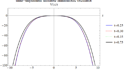
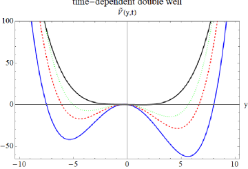
Figure 1: Spectrally equivalent time-dependent anharmonic oscillator potential $V(z,t)$ in (4) and time-dependent double well potential $\tilde{V}(y,t)$ in (2) for $\sigma(t)=\cosh t$, $g(t)=1/4\cosh^{3}t$, $m(t)=(\tanh^{2}t-2)/4$ at different values of time.

3 Conclusions

We have proven the remarkable fact that the time-dependent unstable anharmonic oscillator is spectrally equivalent to a time-dependent double well potential that is bounded from below. The transformations we carried out are summarized as follows:

$$H(z,t)\overset{z\rightarrow x}{\rightarrow}H(x,t)\overset{\text{Dyson}}{\rightarrow}h(x,t)\overset{\text{unitary transform}}{\rightarrow}\hat{h}(x,t)\overset{\text{Fourier}}{\rightarrow}\tilde{h}(y,t).$$

We have first transformed the time-dependent anharmonic oscillator $H(z,t)$ from a complex contour in a Stokes wedge to the real axis $H(x,t)$. The resulting non-Hermitian Hamiltonian $H(x,t)$ was then mapped by mean of a time-dependent Dyson map $\eta(t)$ to a time-dependent Hermitian Hamiltonian $h(x,t)$. It turned out that the Dyson map can not be obtained by simply introducing time-dependence into the known solution for the time-independent case [11], but it required to complexify one of the constants and the inclusion of two additional factors. In order to obtain a potential Hamiltonian we have unitary transformed $h(x,t)$ into a spectrally equivalent Hamiltonian $\hat{h}(x,t)$, which when Fourier transformed leads to $\tilde{h}(y,t)$ that involved a time-dependent double well potential.

A detailed analysis of the spectra and eigenfunctions using approximation methods for time-dependent potential [31] is left for future investigations. Moreover, it is well known that Dyson maps are not unique, in the time-dependent as well as time-independent case, and it might therefore be interesting to explore whether additional spectrally equivalent Hamiltonians to $H(z,t)$ can be found in the same fashion for new type of maps.

Acknowledgments: RT is supported by a City, University of London Research Fellowship.

References

- [1] G. J. Milburn and C. A. Holmes, Dissipative quantum and classical Liouville mechanics of the anharmonic oscillator, Phys. Rev. Lett. 56(21), 2237 (1986).
- [2] G. Gabrielse, H. Dehmelt, and W. Kells, Observation of a relativistic, bistable hysteresis in the cyclotron motion of a single electron, Phys. Rev. Lett. 54(6), 537 (1985).
- [3] R. Seznec and J. Zinn-Justin, Summation of divergent series by order dependent mappings: Application to the anharmonic oscillator and critical exponents in field theory, J. Math. Phys. 20(7), 1398–1408 (1979).
- [4] A. A. Andrianov, The large N expansion as a local perturbation theory, Annals of Physics 140(1), 82–100 (1982).
- [5] S. Graffi and V. Grecchi, The Borel sum of the double-well perturbation series and the Zinn-Justin conjecture, Phys. Lett. B 121(6), 410–414 (1983).
- [6] E. Caliceti, V. Grecchi, and M. Maioli, Double wells: perturbation series summable to the eigenvalues and directly computable approximations, Comm. Math. Phys. 113(4), 625–648 (1988).
- [7] V. Buslaev and V. Grecchi, Equivalence of unstable anharmonic oscillators and double wells, J. of Phys. A: Math. and Gen. 26(20), 5541 (1993).
- [8] C. M. Bender and S. Boettcher, Real Spectra in Non-Hermitian Hamiltonians Having PT Symmetry, Phys. Rev. Lett. 80, 5243–5246 (1998).
- [9] A. Mostafazadeh, Pseudo-Hermitian Representation of Quantum Mechanics, Int. J. Geom. Meth. Mod. Phys. 7, 1191–1306 (2010).
- [10] C. M. Bender, P. E. Dorey, C. Dunning, A. Fring, D. W. Hook, H. F. Jones, S. Kuzhel, G. Levai, and R. Tateo, PT Symmetry: In Quantum and Classical Physics, (World Scientific, Singapore) (2019).
- [11] H. F. Jones and J. Mateo, An Equivalent Hermitian Hamiltonian for the non-Hermitian Potential, Phys. Rev. D73, 085002 (2006).
- [12] C. Figueira de Morisson Faria and A. Fring, Time evolution of non-Hermitian Hamiltonian systems, J. Phys. A39, 9269–9289 (2006).
- [13] A. Mostafazadeh, Time-dependent pseudo-Hermitian Hamiltonians defining a unitary quantum system and uniqueness of the metric operator, Physics Letters B 650(2), 208–212 (2007).
- [14] M. Znojil, Time-dependent version of crypto-Hermitian quantum theory, Physical Review D 78(8), 085003 (2008).
- [15] H. Bíla, Adiabatic time-dependent metrics in PT-symmetric quantum theories, arXiv preprint arXiv:0902.0474 (2009).
- [16] J. Gong and Q.-H. Wang, Time-dependent PT-symmetric quantum mechanics, J. Phys. A: Math. and Theor. 46(48), 485302 (2013).
- [17] A. Fring and M. H. Y. Moussa, Unitary quantum evolution for time-dependent quasi-Hermitian systems with nonobservable Hamiltonians, Phys. Rev. A 93(4), 042114 (2016).
- [18] A. Fring and T. Frith, Exact analytical solutions for time-dependent Hermitian Hamiltonian systems from static unobservable non-Hermitian Hamiltonians, Phys. Rev. A 95, 010102(R) (2017).
- [19] A. Fring and T. Frith, Mending the broken PT-regime via an explicit time-dependent Dyson map, Phys. Lett. A , 2318 (2017).
- [20] A. Mostafazadeh, Energy observable for a quantum system with a dynamical Hilbert space and a global geometric extension of quantum theory, Phys. Rev. D 98(4), 046022 (2018).
- [21] A. Fring and M. H. Y. Moussa, Non-Hermitian Swanson model with a time-dependent metric, Phys. Rev. A 94(4), 042128 (2016).
- [22] A. Fring and T. Frith, Metric versus observable operator representation, higher spin models, Eur. Phys. J. Plus , 133: 57 (2018).
- [23] B. Khantoul, A. Bounames, and M. Maamache, On the invariant method for the time-dependent non-Hermitian Hamiltonians, The European Physical Journal Plus 132(6), 258 (2017).
- [24] M. Maamache, O. K. Djeghiour, N. Mana, and W. Koussa, Pseudo-invariants theory and real phases for systems with non-Hermitian time-dependent Hamiltonians, The European Physical Journal Plus 132(9), 383 (2017).
- [25] J. Cen, A. Fring, and T. Frith, Time-dependent Darboux (supersymmetric) transformations for non-Hermitian quantum systems, J. of Phys. A: Math. and Theor. 52(11), 115302 (2019).
- [26] A. Fring and T. Frith, Solvable two-dimensional time-dependent non-Hermitian quantum systems with infinite dimensional Hilbert space in the broken PT-regime, J. of Phys. A: Math. and Theor. 51(26), 265301 (2018).
- [27] A. Fring and T. Frith, Quasi-exactly solvable quantum systems with explicitly time-dependent Hamiltonians, Phys. Lett. A 383(2-3), 158–163 (2019).
- [28] A. Fring and T. Frith, Eternal life of entropy in non-Hermitian quantum systems, Phys. Rev. A 100(1), 010102 (2019).
- [29] A. Fring and T. Frith, Time-dependent metric for the two-dimensional, non-Hermitian coupled oscillator, Mod. Phys. Lett. A 35(08), 2050041 (2020).
- [30] W. Koussa and M. Maamache, Pseudo-invariant approach for a particle in a complex time-dependent linear potential, Int. J. of Theor. Phys. , 1–14 (2020).
- [31] A. Fring and R. Tenney, Time-independent approximations for time-dependent optical potentials, The European Physical Journal Plus 135(2), 163 (2020).