Electron channeling experiments with bent silicon single crystals - a reanalysis based on a modified Fokker-Planck equation

Abstract

A surprising small dechanneling length was observed at (111) channeling of ultrarelativistic electrons in a 60 $\mu$m thick silicon single crystal with a bending radius of 0.15 m. The experiments were conducted at beam energies between 3.35 and 14 GeV at the Facility for Advanced Accelerator Experimental Tests (FACET at SLAC, USA). It is shown in this paper that the small dechanneling lengths can well be reproduced with a modified Fokker-Planck equation for plane crystals in which a crystal bending has been heuristically introduced. Encouraged by this result experiments have been reconsidered which were performed at the Mainz Microtron MAMI with (110) silicon undulator crystals. The results obtained with the modified Fokker-Planck equation suggest that the observed rather low undulator peak intensity originates from the strongly reduced dechanneling length of electrons in the bent sections of the undulator. A scaling law derived on the basis of the modified Fokker-Planck equation reveals optimized parameters of electron based undulators as possible radiation sources in the $X$- and $\gamma$-ray region.

1 Introduction

The phenomenon of channeling of positively and negatively charged particles plays an important role in the high energy physics domain like for beam bending and collimation [1]. Another intriguing field of research is the development of crystalline undulators for intense radiation production with energies of 100 keV or higher employing relativistic positrons or electrons with energies in the order of a few hundred MeV or more. Such devices were proposed a long time ago [2, 3] and theoretically investigated in detail more recently [4, 5, 6, 7]. A very important prerequisite for an experimental realization of such undulators is the knowledge of the dechanneling length, i.e., the length in which the charged particle remains in an periodically bent crystal in the channel. Of particular interest are electrons since high quality electron beams can much easier be produced as compared to positrons. Currently simulation calculations are widely used to get information on dechanneling lengths, see, e.g., the recent article of A. V. Korol, A. V. Solov’yov et al. [8]. However, also such types of calculations need experimental verifications.

There are principally two possibilities to measure the dechanneling length. The first one is based on a variation of the crystal thickness. However, the results are of little relevance for the goal to construct a crystal undulator radiation source for which the dechanneling length in bent crystals is of interest. Fortunately, there exists a very elegant second possibility, namely to observe dechanneled electrons from a bent crystal. Experiments have been performed at the Facility for Advanced Accelerator Experimental Tests (FACET) at SLAC using a bent silicon single crystal for channeling in the (111) planes at beam energies between 3.35 and 14 GeV [9, 10]. In this paper some of these data will be explained employing the Fokker-Planck equation which has been heuristically modified for bending of the crystal. The aim was to verify a procedure in order to predict dechanneling lengths for the (110) plane of silicon and diamond undulator crystals for experiments at the Mainz microtron facility MAMI at beam energies below 855 MeV.

In the next subsection first the modified Fokker-Planck equation will be described. This section is followed by a comparison of the experimental dechanneling length results of T. N. Wistisen, U. I. Uggerhøj, U. Wienands et al. [10] obtained at FACET (SLAC) with calculations on the basis of the modified Fokker-Planck equation. Encouraged by the good agreement between calculations and experiment a section follows in which dechanneling in bent (110) planes of silicon single crystals will be investigated and compared with previous undulator experiments at MAMI [11, 12]. Finally the question will be addressed which kind of radiation features can be expected from an optimized large amplitude undulator operating with electrons.

Figure 1: Effective potential $U_{eff}=U(y)+U_{cf}(y)$ with $U(y)$ the potential of the (111) planes of a silicon single crystal and $U_{cf}(y)$ the centrifugal potential superimposed. Bending radius $R$ = 0.15 m, electron beam energy 6.3 GeV, interplanar distance $d_{p}$ = 3.135 Å , maximum $U_{m}$ = 33.71 eV at $y_{1}/d_{p}$, maximum $U_{n}$ = 20.54 eV at $y_{2}/d_{p}$. The transverse energy $E_{\perp}$ is schematically also indicated.

2 The modified Fokker-Planck equation for a bent crystal

In figure 1 an example of the effective potential $U_{eff}(y)=U(y)+U_{cf}(y)$ is shown in which a modified Fokker-Planck equation must be solved. The figure depicts a superposition of the potential $U(y)$ for an electron channeling in a straight silicon single crystal with the centrifugal potential

$$U_{cf}(y)=-\frac{\gamma m_{e}c^{2}\beta^{2}}{R}y=-\frac{pv}{R}y$$ (2.1)

which accounts for the bending. Here are $\gamma=1/\sqrt{1-\beta^{2}}$ the Lorentz factor, $\beta=v/c$, $v$ the electron velocity, $c$ the speed of light, $m_{e}$ the rest mass of the electron, $p$ its momentum, and $R$ the bending radius. A coordinate system has been chosen with the $x$ axis pointing into the initial beam direction, and the $y$ axis perpendicular to the channeling plane. The modified Fokker-Planck equation, with $F(x,E_{\perp})=\Delta P/\Delta E_{\perp}$ the probability $\Delta P$ per transverse energy interval $\Delta E_{\perp}$, and $J(x,E_{\perp})=J_{diff}(x,E_{\perp})+J_{drift}(x,E_{\perp})$ the probability current, reads

$$\frac{\partial F(x,E_{\perp})}{\partial x}+\frac{\partial J(x,E_{\perp})}{\partial E_{\perp}}+\theta({E_{\bot}}-{U_{n}})\frac{\partial J_{drift}^{(cf)}(x,E_{\perp})}{\partial E_{\perp}}=0~{},$$ (2.2)

$$J(x,E_{\perp})=-\frac{\partial}{\partial E_{\perp}}\bigg{[}D_{diff}^{(2)}(E_{\perp})F(x,E_{\perp})\bigg{]}+D_{drift}^{(1)}(E_{\perp})F(x,E_{\perp})~{},$$ (2.3)

$$J_{drift}^{(cf)}(x,E_{\perp})=\frac{1}{R}\sqrt{2(E_{\perp}-U_{n})pv}\cdot F(x,E_{\perp})~{}.$$ (2.4)

An additional drift current term $J_{drift}^{(cf)}(x,E_{\perp})$ has been heuristically introduced which accounts for the motion of the probability density $F(x,E_{\perp})$ due to the centrifugal force. It acts directly only on continuum states with $E_{\perp}>U_{n}$. This fact has been expressed by the Heaviside $\theta$ function in equation (2.2). How this term comes about will be explained below.

Details of the basic underlying formalism for the Fokker-Planck equation at planar channeling in straight crystals are described in, e.g., [13, 14, 15] and references cited therein and will not be repeated here. It should only be mentioned that the Fokker-Planck equation in phase space has been simplified assuming statistical equilibrium meaning that the probability distribution of the particle in the channel is assumed to be representable by

$$\frac{dP}{dy}(y,E_{\perp})=\frac{2}{T(E_{\perp})}\sqrt{\frac{\gamma m_{e}}{{2\big{(}E_{\perp}}-U_{eff}(y)\big{)}}}$$ (2.5)

with a time period

$$T(E_{\perp})=2\int\limits_{y_{min}}^{y_{max}}\sqrt{\frac{\gamma m_{e}}{{2\big{(}E_{\perp}}-U_{eff}(y)\big{)}}}~{}~{}dy.$$ (2.6)

The time parameter $T(E_{\perp})$ is the period for one full cycle for a bound state and twice the transit time over the channel for a free state. The limits of the integral $y_{min}$ and $y_{max}$ are roots of the equation $U_{eff}(y)=U(y)+U_{cf}(y)=E_{\perp}$ with $y_{max}=y_{2}$ for $E_{\perp}>U_{n}$, and $y_{min}=y_{1}$ for $E_{\perp}>U_{m}$.

The channeling potential $U(y)$ for the straight crystal has been calculated in the Molière approximation, see e.g. Baier et al. [13, Ch. 9.1 and equation (7.45)]. The electron distribution in the channeling planes has been neglected. Without loss of generality it can be assumed that only the potential in one period, indicated by the vertical dashed lines in figure 1, must be considered for the calculations of the drift coefficient

$$D_{drift}^{(1)}(E_{\perp})=\bigg{\langle}\overline{\frac{\Delta E_{\perp}}{\Delta x}}\bigg{\rangle}_{T}~{},$$ (2.7)

and the diffusion coefficient

$$D_{diff}^{(2)}(E_{\perp})=\frac{1}{2}\bigg{\langle}\frac{\overline{(\Delta E_{\perp})^{2}}}{\Delta x}\bigg{\rangle}_{T}=\bigg{\langle}2\overline{\frac{\Delta E_{\perp}}{\Delta x}}~{}\Big{(}E_{\perp}-U_{eff}(y)\Big{)}\bigg{\rangle}_{T}~{}.$$ (2.8)

Both quantities are mean values with respect to the distribution function equation (2.5) over one period.

The drift coefficient $D_{drift}^{(1)}(E_{\perp})$ has been calculated in the Kitagava-Ohtsuki approximation [16], which accounts for phonon excitation, by means of the integral

$$D_{drift}^{(1)}(E_{\perp})=\frac{E_{s}^{2}}{2pvX_{0}}\frac{2}{T(E_{\perp})c}\frac{1}{2}\sum_{i=1}^{2}\int\limits_{y_{min}}^{y_{max}}\frac{d_{p}}{\sqrt{2\pi}u_{1}}\frac{\exp(-(\eta-y_{i}^{plane})^{2}/2u_{1}^{2})}{\sqrt{2\big{(}E_{\perp}-U_{eff}(\eta)\big{)}/\gamma m_{e}c^{2}}}~{}d\eta.$$ (2.9)

A modified parameter $E_{s}$ = 10.6 MeV has been used in the standard deviation of the Gaussian scattering distribution in the Rossi-Greisen approximation [17, §22 "Multiple Scattering…."] which reads

$$\theta_{0}=\frac{10.6~{}\mbox{MeV}}{pv}\sqrt{\frac{x}{X_{0}}}~{},$$ (2.10)

for the reasoning see [18, footnote in chapter 3]. The quantity $X_{0}$ = 0.0936 m is the radiation length of silicon, and $u_{1}$ = 0.076 Å  the standard deviation of the thermal vibration amplitude. The quantity $d_{p}=a/\sqrt{3}$ = 3.135 Å  in the nominator of the integral is the interplanar distance, with $a$ = 5.431 Å  the lattice constant of silicon at 300 K. It should be mentioned that in case of (111) geometry two planes account for the potential minima which are $\Delta^{pot}$ = 0.7515 Å  apart. The lattice planes have a distance of $\Delta^{plane}=a/(4\sqrt{3})$ = 0.7839 Å. Since the minimum of the potential $U(y)$ was shifted to $y$ = 0, the $y_{i}^{plane}$ read $y_{1}^{plane}=(\Delta^{plane}-\Delta^{pot})/2$, and $y_{2}^{plane}=-(\Delta^{plane}+\Delta^{pot})/2$. The factor 1/2 in front of the sum in equation (2.9) accounts for a proper normalization since each of the exponential functions is normalized to one.

The diffusion coefficient $D_{diff}^{(2)}(E_{\perp})$ has been calculated by means of the equation

$$\frac{\partial}{\partial E_{\perp}}\Big{[}T(E_{\perp})\cdot D_{diff}^{(2)}({E_{\perp})}\Big{]}=T(E_{\perp})\cdot D_{drift}^{(1)}(E_{\perp}),$$ (2.11)

i.e., by integration of the known right hand side of this equation and division by $T(E_{\perp})$. Examples for $T(E_{\perp})$, $D_{drift}^{(1)}(E_{\perp})$, and $D_{diff}^{(2)}(E_{\perp})$ are shown in figure 2 (a-c).

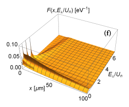
Figure 2: (a) Time parameter $Tc$, (b) drift coefficient $D_{drift}^{(1)}$, (c) diffusion coefficient $D_{diff}^{(2)}$, (d) drift coefficient $D_{drift}^{(cf)}$ due to centrifugal force, (e) initial distribution $F_{0}$ at $x=0$ all as function of normalized transverse energy $E_{\perp}/U_{n}$, and (f) numerical solution $F(x,E_{\perp}/U_{n})$ of the modified Fokker-Planck equation. Calculations for beam energy $E$ = 6.3 GeV, bending radius $R$ = 0.15 m, standard deviation $\sigma^{\prime}_{y}=10~{}\mu$rad for angular divergence of the electron beam, and $U_{n}$ = 20.54 eV.

Let us turn to the question how the additional drift current term in equation (2.2) comes about. In principle, the probability density $F(x,y,E_{\perp})$ depends on three variables. However, a particle which enters into the continuum at $x=x_{0}$ moves, viewed from the bent channel which is assumed to be straight, on a circle with radius $R$ which can be approximated by the equation $y=(x-x_{0})^{2}/2R$. The transverse energy $E_{\perp}=U_{n}+pv/R\cdot y$ is translational invariant with respect to $x_{0}$, i.e., $E_{\perp}$ evolves as function of $y$ irrespective of the depth $x_{0}$ at which the particle leaves the channel. Therefore the variable $y$ can be eliminated leading to $E_{\perp}=U_{n}+(pv/R)\cdot(x-x_{0})^{2}/2R$. The additional probability current is expressed as $J_{drift}^{(cf)}(x,E_{\perp})=\partial E_{\perp}(x)/\partial x\cdot F(x,E_{\perp})$ which leads with $\partial E_{\perp}(x)/\partial x=pv(x-x_{0})/R^{2}$, and $x-x_{0}=R\sqrt{2(E_{\perp}-U_{n})/pv}$ to equation (2.4).

One may introduce the drift coefficient

$$D_{drift}^{(cf)}(E_{\perp})=\frac{1}{R}\sqrt{2(E_{\perp}-U_{n})\cdot pv}$$ (2.12)

which accounts for the motion of the probability density $F(x,E_{\perp})$ due to the centrifugal force. It is shown in figure 2 (d). The additional drift coefficient does not act on bound states with $E_{\perp}<U_{n}$.

For the initial conditions at $x=0$, required for the numerical solution of the Fokker-Planck equation, a uniform distribution of the electron across the transverse $y$ coordinate, and a Gaussian scattering distribution tilted by an angle $\psi^{0}_{in}$, and with standard deviation $\sigma^{\prime}_{y}$ for the angular divergence were assumed. For a function with the two random variables $y_{in}$ and $\psi_{in}$, which are connected to $E_{\perp}$ by the relation $E_{\perp}/U_{0}=U_{eff}(y_{in})/U_{0}+(\psi_{in}/\psi_{c}-\psi^{0}_{in}/\psi_{c})^{2}$, with $\psi_{c}=\sqrt{2U_{0}/\gamma m_{e}c^{2}}$ the critical angle for a potential depth $U_{0}$ = 25.15 eV, the formalism described in Ref. [19, chapter 6] was applied. This approach leads to the probability density

$$F_{0}(E_{\perp})~{}=\frac{1}{2\sqrt{2\pi}(\sigma^{\prime}_{y}/\psi_{c})U_{0}}\int\limits_{y_{min}}^{y_{max}}\Bigg{(}\frac{\exp\bigg{[}-\frac{\big{(}\sqrt{(E_{\perp}-U_{eff}(\eta))/U_{0}}+\psi_{in}^{0}/\psi_{c}\big{)}^{2}}{2(\sigma^{\prime}_{y}/\psi_{c})^{2}}\bigg{]}}{\sqrt{(E_{\perp}-U_{eff}(\eta))/U_{0}}}~{}+$$ (2.13)

$$+\frac{\exp\bigg{[}-\frac{\big{(}-\sqrt{(E_{\perp}-U_{eff}(\eta))/U_{0}}+\psi_{in}^{0}/\psi_{c}\big{)}^{2}}{2(\sigma^{\prime}_{y}/\psi_{c})^{2}}\bigg{]}}{\sqrt{(E_{\perp}-U_{eff}(\eta))/U_{0}}}\Bigg{)}~{}d\eta.$$

The initial distribution with parameters described in the caption is shown in figure 2 (e). A fraction of 64.5 % is captured in a bound state with $E_{\perp}<U_{n}$.

The probability density $F(x,E_{\perp})$ of a free particle moves as function of $x$ rapidly into the $E_{\perp}$ direction while preserving normalization. This fact can be seen in figure 2 (f) by the ridge which originates from the primary unbound density at $E_{\perp}/U_{n}\approx 1.64$ of the initial distribution, see figure 2 (e). While the particle moves over the region with $y>y_{2}$, see figure 1, volume capture may happen which is not included in the calculations. For $E_{\perp}~{}>~{}U_{m}$ the particle may also enter via the diffusion term in the Fokker-Planck equation into the region with $y<y_{1}$ in which it may also experience volume capture (rechanneling). This possibility has been neglected as well. Therefore, the results for the dechanneling length calculations represent lower limits which should be taken in mind when compared with experimental results.

3 Comparison of dechanneling length measurements with results of the modified Fokker-Planck equation for bent crystals

As already mentioned in the Introduction, dechanneling length measurements have been performed at FACET (SLAC) for Si (111) planes at beam energies between 3.35 and 14 GeV [10]. The crystal thickness and the bending radius $R$ were 60 $\mu$m and 0.15 m, respectively. In figure 3 (a) an example of calculations on the basis of the modified Fokker-Planck equation (2.2-2.4) is shown. It can be seen that the occupation of the potential pocket $f_{ch}(x)$ can well be approximated by an exponential function. With the exception of an unimportant scaling factor no further parameters were adapted. The dechanneling lengths $L_{d}$ obtained this way are compared in figure 3 (b) with the experimental results [10]. The gross features of the measurements are well described. Shown are also calculations on the basis of the MBN Explorer software package [20].

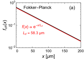
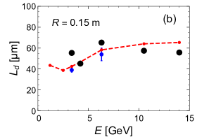
Figure 3: (a) Solution of the modified Fokker-Planck equation (black line) compared with an exponential decay (red line). Shown is the fraction of electrons captured in the potential pocket $f_{ch}(x)$ as function of the distance $x$ traversed by the electron. The dechanneling length $L_{d}$ was adapted. Beam energy 6.3 GeV. (b) Comparison of the dechanneling lengths obtained this way (red points) with experimental results (full circles) [10]. The red dashed lines connect the calculated red points to guide the eye. The blue error bars are simulation calculations of G. B. Sushko , A. V. Korol, A. V. Solov^′yov [20] on the basis of the MBN Explorer software package.

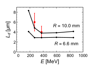
Figure 4: Comparison of the calculated dechanneling length as function of the beam energy with results extracted from experiments at MAMI [11, 12]. The design value of the bending radius was $R$ = 6.6 mm. Shown are also calculations for $R$ = 10 mm which seem to be in better agreement with experiments (red error bars).

Encouraged by this result calculations have been performed for a Si (110) four period undulator with which experiments were performed at MAMI beam energies of 270 and 375 MeV [11, 12]. The design values were $\lambda_{U}=9.9~{}\mu$m for the period length, and $A=4.64$ Å  for the amplitude, resulting in a bending radius $R\cong(\lambda_{U}/4)^{2}/2A$ = 6.6 mm. In figure 4 the solutions of the modified Fokker-Planck equation as function of the beam energy are compared with the experimental results. It appears that for the real undulator a bending radius $R$ = 10 mm might be a better approximation. However, the experimental finding in references [11, 12] that only a few percent of all electrons contribute to the coherent part of the peak strongly suggests that only parts of the undulator exhibit the designed structure.

4 Scaling behaviour of the modified Fokker-Planck equation

After all what has been addressed in the previous sections one might ask the question what can be expected from an optimized large amplitude undulator operating with electrons. In principle, this question can be answered solving the modified Fokker-Planck equation in the parameter space $\lambda_{U}$, amplitude $A$, electron energy $E$, and number of periods $N_{U}$ by a brute-force approach. However, in the following this issue has been approached by investigating the scaling behaviour of the modified Fokker-Planck equation (2.2-2.4) which can be rewritten as

$$\frac{{\partial F(x,{E_{\bot}})}}{{\partial x}}+\theta({E_{\bot}}-{U_{n}})\frac{\partial}{{\partial{E_{\bot}}}}\left[\frac{1}{R}\sqrt{2({E_{\bot}}-{U_{n}})pv}\;F(x,{E_{\bot}})\right]=$$

$$=\frac{\partial}{{\partial{E_{\bot}}}}\left[{D_{diff}^{(2)}({E_{\bot}})T({E_{\bot}})\frac{\partial}{{\partial{E_{\bot}}}}\frac{{F(x,{E_{\bot}})}}{{T({E_{\bot}})}}}\right].$$ (4.1)

The same equation with the perpendicular energy variable $E_{\bot}$ normalized to $U_{0}$ and the crystal thickness variable $x$ normalized to the dechanneling length $L^{R\rightarrow\infty}_{de}$ for a bending radius $R\rightarrow\infty$ reads

$$\frac{{\partial F(x/L_{de}^{R\to\infty},{E_{\bot}}/{U_{0}})}}{{\partial x/L_{de}^{R\to\infty}}}+\theta\left(\frac{E_{\bot}-U_{n}}{U_{0}}\right)\frac{{L_{de}^{R\to\infty}}}{R}\sqrt{\frac{{2pv}}{{{U_{0}}}}}\frac{\partial}{{\partial{E_{\bot}}/{U_{0}}}}\left(\sqrt{\frac{E_{\bot}-U_{n}}{U_{0}}}\;F(x/L_{de}^{R\to\infty},{E_{\bot}}/{U_{0}})\right)=$$

$$=\frac{\partial}{{\partial{E_{\bot}}/{U_{0}}}}\left[{D_{diff}^{(2)}({E_{\bot}}/{U_{0}})\;T({E_{\bot}}/{U_{0}})\frac{\partial}{{\partial{E_{\bot}}/{U_{0}}}}\left(\frac{{F(x/L_{de}^{R\to\infty},{E_{\bot}}/{U_{0}})}}{{T({E_{\bot}}/{U_{0}})}}\right)}\right]\;\;\;\;\;\;\;$$ (4.2)

with

$$L_{de}^{R\to\infty}=2\frac{{{U_{0}}\;pv\;{X_{0}}}}{{E_{s}^{2}}}.$$ (4.3)

The latter is exactly the expression which Baier et al. quote [13, equation (10.1)]. However, the expression $E_{s,Baier}=\sqrt{2\pi}m/e={{15.0\;{\rm{MeV}}}}$ must be replaced for small thicknesses $x\ll X_{0}$ by our empirical $E_{s}$ = 10.6 MeV. For Si (110) the barrier hight can well be approximated in the interval $0\leq a_{n}R_{c}/R<0.4$ by $U_{n}/U_{0}=(1-a_{n}R_{c}/R)^{3.5}$ with $a_{n}=0.696$ and the critical radius $R_{c}=a_{c}\cdot pv$ with $a_{c}$ = 1.69 mm/GeV. Introducing normalized variables

$$\Upsilon=\frac{L_{d}}{L_{d}^{R\to\infty}}=\frac{L_{de}}{2U_{0}X_{0}R_{c}/(a_{c}E_{s}^{2})}~{}~{}~{}~{}~{}~{}~{}~{}~{}\mbox{and}~{}~{}~{}~{}~{}~{}~{}~{}~{}\Lambda=\frac{{L_{de}^{R\to\infty}}}{R}\sqrt{\frac{{2pv}}{{{U_{0}}}}}=\frac{\sqrt{8U_{0}}}{E_{s}^{2}}\frac{X_{0}}{a_{c}^{3/2}}\frac{R_{c}^{3/2}}{R},$$ (4.4)

which both exhibit a functional dependence on the critical radius $R_{c}$, the dechanneling length can be represented as shown in figure 5 (a). The black curve is a best fit with the function

$$\Upsilon(\Lambda)=\frac{{{L_{d}}(\Lambda)}}{{L_{de}^{R\to\infty}}}=\frac{C_{\Lambda}}{{{{(\Lambda-{\Lambda_{0}})}^{2/3}}}}.$$ (4.5)

The parameters $C_{\Lambda}$ and $\Lambda_{0}$ are quoted in figure 5 (a). Within the limits $4\lesssim\Lambda\lesssim 50$ of the validity of this approximation the dechanneling length can be calculated with equation (4.5) for arbitrary combinations of $pv$, and $R$ at fixed $U_{0}=22.56$ eV, $X_{0}=0.0936$ m, and $E_{s}=10.6$ MeV.

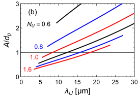
Figure 5: (a) Dechanneling length $L_{d}$ as obtained from various numerical solutions of the Fokker-Planck equation depicted in normalized variables as defined by equation (4.4). The black curve is a best fit with equation (4.5). (b) Amplitude $A/d_{p}$ normalized to the (110) inter planar distance $d_{p}$ = 1.919 Å  for a silicon single crystal as function of the undulator period $\lambda_{U}$. Beam energy 855 MeV. The bending radius $R$ has been varied in the limits defined by $0\leq a_{n}R_{c}/R<0.4$ with $a_{n}$ = 0.696. From the equidistance parameter characteristics for $N_{U}$ the number of meaningful undulator periods can be estimated. For a large amplitude undulator $A/d_{p}\geq 1$ is required.

5 Discussion and conclusion

With the parametrization described in the previous section 4 one might now be able to seek for optimal parameters for a large amplitude undulator as follows. The undulator period $\lambda_{U}$, maximum number of periods $N_{U}$, and the dechanneling length $L_{d}(\Lambda)$ should obey the equation $N_{U}\lambda_{U}=2L_{d}(\Lambda)$. From simple geometrical considerations one obtains for the amplitude $A\cong(\lambda_{U}/4)^{2}/2R$. Combining both equations results in the tuple

$$\Bigg{(}\lambda_{U}=\frac{2L_{d}\big{(}\Lambda(pv,R)\big{)}}{N_{U}},~{}~{}~{}~{}\frac{A}{d_{p}}=\frac{1}{8}\frac{{L_{d}^{2}\big{(}\Lambda(pv,R)\big{)}}}{{R\;{d_{p}}N_{U}^{2}}}\Bigg{)}$$ (5.1)

which is shown in figure 5 (b) for $pv\cong pc$ = 855 MeV, corresponding to $R_{c}$ = 1.445 mm, with $N_{U}$ as a parameter. The bending radius $R$ has been varied in the limits defined by $0\leq a_{n}R_{c}/R<0.4$. The requirement $A/d_{p}\geq 1$ for a large amplitude undulator, $d_{p}$ = 1.919 Å  is the (110) inter planar distance of a silicon single crystal, shows that the coherence length in the investigated parameter space of $\Lambda(pv,R)$ amounts to less than two periods. In other words, neglecting rechanneling it makes no sense to produce at $\lambda_{U}=9.9~{}\mu$m an undulator with more than about two periods, and at $\lambda_{U}=20~{}\mu$m with more than about three periods. However, since rechanneling enhances the intensity, many more periods may be advantageous. Although one cannot tell at this stage of the analysis something about the intensity of the emitted undulator radiation, it seems to be quite probable that the design values for the above analyzed $\lambda_{U}=9.9~{}\mu$m four-period undulator with $A/d_{p}=2.42$ were not optimal since the coherence length amounts to only 0.57 periods.

An increase of the beam energy may be beneficial although the dependence on the beam energy turned out to be rather weak. For instance, at 14 GeV the coherence length might be at $A/d_{p}=1$ and $\lambda_{U}=150~{}\mu$m close to four periods. The associated undulator parameter is $K=2\pi\gamma A/\lambda_{U}$ = 0.22. Under these circumstances an undulator with 10 periods or more, if advantage will be taken on rechanneling, might emit rather intense radiation with a photon energy of about 12.4 MeV at on-axis observation. Such a device may well be worth for further investigation.

References

- [1] J. R. A. Carrigan, Negative Particle Planar and Axial Channeling and Channeling Collimation, in Charged and Neutral Particles Channeling Phenomena, Channeling 2008, Proceedings of the 51st Workshop of the INFN ELOISATRON Project, Erice, Italy 15 October - 1 November 2008, S. B. Dabagov, L. Palumbo and A. Zichichi, eds., The Science and Culture Series - Physics, (World Scientific Publishing Co. Pte. Ltd., 5 Toh Tuck Link, Singapore 596224), pp. 129–143, World Scientific: New Jersey, London, Singapore, Beijing, Shanghai, Hong Kong, Taipei, Chennai, 2008.
- [2] V. V. Kaplin, S. V. Plotnikov and S. A. Vorob’ev, Radiation by charged particles channeled in deformed crystals, English Translation: Soviet Physics - Technical Physics 25 (1980) 650 .
- [3] V. G. Baryshevsky and A. O. G. I. Ya. Dubovskaya, Generation of - Quanta by Channeled Particles in the Presence of a Variable External Field, Physics Letters A 77 (1980) 61.
- [4] A. V. Korol, A. V. Solov’yov and W. Greiner, Channeling of Positrons through Periodically Bent Crystals: on the Feasibility of Crystalline Undulator and Gamma-Laser, International Journal of Modern Physics E 13 (2004) 867.
- [5] S. Bellucci and V. A. Maisheev, Radiation of relativistic particles for quasiperiodic motion in a transparent medium, Journal of Physics: Condensed Matter 18 (2006) S2083.
- [6] V. G. Baryshevsky, High-Energy Nuclear Optics of Polarized Particles. World Scientific New Jersey, London, Singapore, Beijing, Shanghai, Hong Kong, Taipei, Chennai, World Scientific Publishing Co. Pte. Ltd., 5 Toh Tuck Link, Singapore 596224, 2012.
- [7] A. V. Korol, A. V. Solov’yov and W. Greiner, Channeling and Radiation in Periodically Bent Crystals. Springer Heidelberg, New York, Dordrecht, London, Springer-Verlag Berlin Heidelberg 2013, 2013.
- [8] A. V. Korol, V. G. Bezchastnov, G. B. Sushko and A. V. Solov’yov, Simulation of channeling and radiation of 855 MeV electrons and positrons in a small-amplitude short-period bent crystal, Nuclear Instruments and Methods in Physics Research B 387 (2016) 41.
- [9] A. Mazzolari, E. Bagli, L. Bandiera, V. Guidi, H. Backe, W. Lauth et al., Steering of a Sub-GeV Electron Beam through Planar Channeling Enhanced by Rechanneling, Physical Review Letters 112 (2014) 135503.
- [10] T. N. Wistisen, U. I. Uggerhøj, U. Wienands, T. W. Markiewicz, R. J. Noble, B. C. Benson et al., Channeling, volume reflection, and volume capture study of electrons in a bent silicon crystal, Physical Review Accelerators and Beams 19 (2016) 071001 11 pages.
- [11] H. Backe, D. Krambrich, W. Lauth, K. Andersen, J. L. Hansen and U. I. Uggerhøj, Radiation emission at channeling of electrons in a strained layer Si1-xGex undulator crystal, Nuclear Instruments and Methods in Physics Research B 309 (2013) 37 .
- [12] H. Backe, D. Krambrich, W. Lauth, K. K. Andersen, J. L. Hansen and U. I. Uggerhøj, Channeling and Radiation of Electrons in Silicon Single Crystals and Si1-xGex Crystalline Undulators, Journal of Physics: Conference Series 438 (2013) 012017.
- [13] V. N. Baier, V. M. Katkov and V. M. Strakhovenko, Electromagnetic Processes at High Energies in Oriented Single Crystals. World Scientific, Singapore, New Jersey, London, HongKong, World Scientific Publishing Co. Pte. Ltd, P O Box 128, Farrer Road, Singapore 912805, 1998.
- [14] V. V. Beloshitsky and C. G. Trikalinos, Passage and radiation of relativistic channeled particles, Radiation Effects 56 (1981) 71.
- [15] M. A. Kumakhov and F. F. Komarov, Radiation from charged particles in solids. American Institute of Physics New York, , 1989.
- [16] M. Kitagawa and Y. H. Ohtsuki, Modified Dechanneling Theory and Diffusion Coefficients, Physical Review B 8 (1973) 3117 .
- [17] B. Rossi and K. Greisen, Cosmic-Ray Theory, Review of Modern Physics 13 (1941) 240.
- [18] H. Backe and W. Lauth, Channeling experiments with sub-GeV electrons in flat silicon single crystals, Nuclear Instruments and Methods in Physics Research B 355 (2015) 24.
- [19] A. Papoulis, Probability, Random Variables, and Stochastic Processes. McGraw-Hill Book Company Auckland, Bogotá, Guatemala, Hamburg, Lisbon,London, Madrit, Mexico, New Dehli Panama, Paris, San Juan, Sáo Paulo, Singapore, Sydney, Tokyo, , 1989.
- [20] G. B. Sushko, A. V. Korol and A. V. Solov’yov, Multi-GeV electron and positron channeling in bent silicon crystals, Nuclear Instruments and Methods in Physics Research B 355 (2015) 39.