Quantum Dynamics on the three-dimensional $q$-deformed Euclidean Space

Abstract

I extend the three-dimensional $q$-deformed Euclidean space by a time element and discuss the algebraic structure of this quantum space together with its differential calculi. Using the star-product formalism, I will give basic operations of $q$-deformed analysis for the $q$-deformed Euclidean space with a time element. I show that the time-evolution operator of a quantum system living in the $q$-deformed Euclidean space is of the same form as in the undeformed case. The reasonings also show that the well-known methods of quantum dynamics apply to quantum systems living in the $q$-deformed Euclidean space.

1 Introduction

Several arguments say that space and time are discrete on a fundamental level [1, 2, 3, 4, 5]. To answer the question of whether space and time are continuous or discrete, you need to find out how the assumption of a discrete space-time changes physical laws. The $q$-deformed Euclidean space provides a mathematical framework to investigate this question [6, 7].

In Ref. [8], I have begun to develop a formalism for the quantum-theoretical description of free particles existing in the $q$-deformed Euclidean space. In the present article, I will continue these considerations and focus on the question of how to describe the time evolution of a $q$-deformed quantum system. To this end, you need a $q$-deformed space that has a time element. Considering a $q$-analog of Minkowski space could be one way for this task [9, 10, 7]. The $q$-deformed Minkowski space, however, has a very complex structure making calculations very time-consuming. Therefore, I am going to choose a different way in this article, i. e., I extend the algebra of the $q$-deformed Euclidean space by an element behaving like a commutative parameter.

Now, I am going to describe the contents of the various sections in more detail. Chap. 2 summarizes the algebraic basis for an understanding of the $q$-deformed Euclidean space. In Chap. 3, I show how to extend the algebra of the $q$-deformed Euclidean space by an element that commutes with all coordinate generators of the $q$-deformed Euclidean space and behaves like a scalar concerning the Hopf algebra $\mathcal{U}_{q}(\operatorname*{su}\nolimits_{2})$. Due to its properties, the new element functions as a time element. Furthermore, I will show how to extend the two differential calculi of the $q$-deformed Euclidean space by a partial derivative for the time element.

To formulate equations of motion on the $q$-deformed Euclidean space, we need some tools of a $q$-deformed multidimensional analysis. For this purpose, we associate the $q$-deformed Euclidean space with a commutative coordinate algebra by using the star-product formalism. In doing so, you can calculate formulas for star-products, $q$-derivatives, $q$-integrals as well as $q$-translations and $q$-exponentials [11, 12, 13, 14, 15]. In Chap. 4, I will briefly explain the corresponding considerations and apply them to the Euclidean quantum space supplemented by a time element. Since the time element behaves like a commutative parameter and is independent of the space coordinates, the following situation arises: The formulas derived for the Euclidean quantum space in my previous work remain valid, and the operations concerning the time element are of the same form as in the undeformed case.

Chap. 5 shows you can perform time displacements in the $q$-deformed Euclidean space in the same way as in the undeformed case. Consequently, the time-evolution operator for a physical system existing in the $q$-deformed Euclidean space is of the same form as in the undeformed case. Due to this fact, we can apply the well-known methods for describing the time development of a physical system to the $q$-deformed Euclidean space. In Chap. 6, you can see, in particular, that the Schrödinger equation and the Heisenberg equation of motion apply again.

2 The three-dimensional $q$-deformed Euclidean space

The three-dimensional $q$-deformed Euclidean space $\mathbb{R}_{q}^{3}$ is a three-dimensional representation of the Drinfeld-Jimbo algebra $\mathcal{U}_{q}(\operatorname*{su}_{2})$ [16, 17, 18, 19]. The latter is a deformation of the universal enveloping algebra of the Lie algebra $\operatorname*{su}_{2}$. Accordingly, the algebra $\mathcal{U}_{q}(\operatorname*{su}_{2})$ has three generators $T^{+}$, $T^{-}$, and $T^{3}$ which satisfy the following relations [10]:

$$q^{-1}\hskip 0.72229ptT^{+}T^{-}-q\,T^{-}T^{+} =T^{3},$$

$$q^{\hskip 0.72229pt2}\hskip 0.72229ptT^{3}T^{+}-q^{-2}\hskip 0.72229ptT^{+}T^{3} =(q+q^{-1})\hskip 0.72229ptT^{+},$$

$$q^{\hskip 0.72229pt2}\hskip 0.72229ptT^{-}T^{3}-q^{-2}\hskip 0.72229ptT^{3}T^{-} =(q+q^{-1})\hskip 0.72229ptT^{-}.$$ (1)

The algebra $\mathcal{U}_{q}(\operatorname*{su}\nolimits_{2})$ has a Casimir operator, i. e. an element that commutes with the generators $T^{+}$, $T^{-}$, and $T^{3}$ [20]:

$$\vec{T}^{\hskip 0.72229pt2}=q^{\hskip 0.72229pt2}\lambda^{-2}\tau^{1/2}+\lambda^{-2}\tau^{-1/2}+\tau^{-1/2}\hskip 0.72229ptT^{+}T^{-}-q\hskip 0.72229pt\lambda^{-2}\lambda_{+}.$$ (2)

Note that we have introduced the element

$$\tau=1-\lambda T^{3}$$ (3)

and the constants

$$\lambda=q-q^{-1},\qquad\lambda_{+}=q+q^{-1}.$$ (4)

The different representations of $\mathcal{U}_{q}(\operatorname*{su}\nolimits_{2})$ are distinguished by the eigenvalues of the Casimir operator in Eq. (2) and the states of the same representation are distinguished by the eigenvalues of the generator $T^{3}$. If we label the eigenvalues of $\vec{T}^{2}$ with $j$ and those of $T^{3}$ with $m$ then we have for each $j=0,\frac{1}{2},1,\ldots$ a $(2\hskip 0.72229ptj+1)$-dimensional irreducible representation with the states $\left|\hskip 0.72229ptj,m\right\rangle,$ $m\in\left\{-j,-j+1,\ldots,j-1,j\right\}$. For the actions of the generators of $\mathcal{U}_{q}(\operatorname*{su}\nolimits_{2})$ on the states $\left|\hskip 0.72229ptj,m\right\rangle$ applies [10]:

$$\vec{T}^{\hskip 0.72229pt2}\left|\hskip 0.72229ptj,m\right\rangle =[[\hskip 0.72229ptj]]_{q^{-2}}[[\hskip 0.72229ptj+1]]_{q^{2}}\left|\hskip 0.72229ptj,m\right\rangle,$$

$$T^{3}\left|\hskip 0.72229ptj,m\right\rangle =q^{-1}[[2\hskip 0.72229ptm]]_{q^{-2}}\left|\hskip 0.72229ptj,m\right\rangle,$$ (5)

$$T^{+}\left|\hskip 0.72229ptj,m\right\rangle =q^{-1}\sqrt{[[\hskip 0.72229ptj+m+1]]_{q^{-2}}[[\hskip 0.72229ptj-m]]_{q^{2}}}\left|\hskip 0.72229ptj,m+1\right\rangle,$$

$$T^{-}\left|\hskip 0.72229ptj,m\right\rangle =q\sqrt{[[\hskip 0.72229ptj+m]]_{q^{-2}}[[\hskip 0.72229ptj-m+1]]_{q^{2}}}\left|\hskip 0.72229ptj,m-1\right\rangle.$$ (6)

The expressions above depend on the so-called antisymmetric $q$-numbers, which are defined as follows:

$$[[n]]_{q}=\frac{1-q^{n}}{1-q}.$$ (7)

The states of the $\mathcal{U}_{q}(\operatorname*{su}_{2})$-triplet form the coordinates of the three-dimensional Euclidean quantum space $\mathbb{R}_{q}^{3}$:

$$X^{-}=\left|1,-1\right\rangle,\qquad X^{3}=\left|1,0\right\rangle,\qquad X^{+}=\left|1,1\right\rangle.$$ (8)

Thus, we obtain the actions of the $\mathcal{U}_{q}(\operatorname*{su}_{2})$-generators on the coordinates $X^{+}$, $X^{3}$, and $X^{-}$ from the identities in Eqs. (5) and (6) if we choose $j=1$ and take into account the identifications of Eq. (8):

$$T^{-}\triangleright X^{-} =0,$$

$$T^{-}\triangleright X^{3} =q^{3/2}\lambda_{+}^{1/2}X^{-},$$

$$T^{-}\triangleright X^{+} =q^{1/2}\lambda_{+}^{1/2}X^{3},$$ (9)

$$T^{3}\triangleright X^{-} =-q^{2}\lambda_{+}\hskip 0.72229ptX^{-},$$

$$T^{3}\triangleright X^{3} =0,$$

$$T^{3}\triangleright X^{+} =q^{-2}\lambda_{+}\hskip 0.72229ptX^{+},$$ (10)

$$T^{+}\triangleright X^{-} =q^{-1/2}\lambda_{+}^{1/2}X^{3},$$

$$T^{+}\triangleright X^{3} =q^{-3/2}\lambda_{+}^{1/2}X^{+},$$

$$T^{+}\triangleright X^{+} =0.$$ (11)

In this respect, the quantum space $\mathbb{R}_{q}^{3}$ forms a left module of the Hopf algebra $\mathcal{U}_{q}(\operatorname*{su}_{2})$.

The Drinfeld-Jimbo algebra $\mathcal{U}_{q}(\operatorname*{su}_{2})$ is a Hopf algebra as well [21]. For this reason, it has a mapping $\Delta:\mathcal{U}_{q}(\operatorname*{su}_{2})\rightarrow\mathcal{U}_{q}(\operatorname*{su}_{2})\otimes\mathcal{U}_{q}(\operatorname*{su}_{2})$ called coproduct. On the generators of $\mathcal{U}_{q}(\operatorname*{su}_{2})$, the co-product reads as follows [22, 20]:

$$\Delta(T^{+}) =T^{+}\otimes 1+\tau^{1/2}\otimes T^{+},$$

$$\Delta(T^{-}) =T^{-}\otimes 1+\tau^{1/2}\otimes T^{-},$$

$$\Delta(T^{3}) =T^{3}\otimes 1+\tau\otimes T^{3}.$$ (12)

Being a Hopf algebra, $\mathcal{U}_{q}(\operatorname*{su}_{2})$ has an antipode $S:\mathcal{U}_{q}(\operatorname*{su}_{2})\rightarrow$ $\mathcal{U}_{q}(\operatorname*{su}_{2})$ and a co-unit $\varepsilon:\mathcal{U}_{q}(\operatorname*{su}_{2})\rightarrow\mathbb{C}$ as well. For the antipode applies

$$S(T^{\pm})=-\hskip 0.72229pt\tau^{-1/2}\hskip 0.72229ptT^{\pm},\qquad S(T^{3})=-\hskip 0.72229pt\tau^{-1}T^{3}.$$ (13)

The co-units of the generators $T^{+}$, $T^{-}$, and $T^{3}$ are equal to zero:

$$\varepsilon(T^{+})=\varepsilon(T^{-})=\varepsilon(T^{3})=0.$$ (14)

The coproduct of $\mathcal{U}_{q}(\operatorname*{su}_{2})$ determines the commutation relations between the generators of the Hopf algebra $\mathcal{U}_{q}(\operatorname*{su}_{2})$ and the coordinates of the Euclidean quantum space $\mathbb{R}_{q}^{3}$ since we have

$$h\hskip 0.72229ptv=\left(h_{\left(1\right)}\triangleright v\right)h_{\left(2\right)}\quad\text{for}\quad h\in\mathcal{U}_{q}(\operatorname*{su}\nolimits_{2}),\quad v\in\mathbb{R}_{q}^{3}.$$ (15)

Note that we have written the coproduct in the so-called Sweedler notation, i. e. $\Delta(h)=h_{\left(1\right)}\otimes h_{\left(2\right)}$. Taking into account the actions in Eqs. (9)-(11) as well as the expressions in Eq. (12), the above identity leads to the following commutation relations [7]:

$$T^{-}X^{-} =q^{2}X^{-}T^{-},$$

$$T^{-}X^{3} =X^{3}\hskip 0.72229ptT^{-}+\hskip 0.72229ptq^{3/2}\lambda_{+}^{1/2}X^{-},$$

$$T^{-}X^{+} =q^{-2}X^{+}T^{-}+\hskip 0.72229ptq^{1/2}\lambda_{+}^{1/2}X^{3},$$ (16)

$$T^{3}X^{-} =q^{4}X^{-}T^{3}-q^{2}\lambda_{+}\hskip 0.72229ptX^{-},$$

$$T^{3}X^{3} =X^{3}\hskip 0.72229ptT^{3},$$

$$T^{3}X^{+} =q^{-4}X^{+}T^{3}+q^{-2}\lambda_{+}\hskip 0.72229ptX^{+},$$ (17)

$$T^{+}X^{-} =q^{2}X^{-}T^{+}+\hskip 0.72229ptq^{-1/2}\lambda_{+}^{1/2}X^{3},$$

$$T^{+}X^{3} =X^{3}\hskip 0.72229ptT^{+}+\hskip 0.72229ptq^{-3/2}\lambda_{+}^{1/2}X^{+},$$

$$T^{+}X^{+} =q^{-2}X^{+}T^{+}.$$ (18)

The three generators $X^{+}$, $X^{3}$, and $X^{-}$ of the quantum space $\mathbb{R}_{q}^{3}$ are subject to the following commutation relations [7]:

$$X^{3}X^{+}-q^{2}X^{+}X^{3}=0,$$

$$X^{3}X^{-}-q^{-2}X^{-}X^{3}=0,$$

$$X^{-}X^{+}-X^{+}X^{-}-(q-q^{-1})\hskip 0.72229ptX^{3}X^{3}=0.$$ (19)

The relations above are completely determined by the requirement that they have to be compatible with the commutations relations in Eqs. (16)-(18). For example, it must hold for all $A\in\{+,3,-\}$:

$$T^{A}(X^{3}X^{+}-q^{2}X^{+}X^{3})=(X^{3}X^{+}-q^{2}X^{+}X^{3})\hskip 0.72229ptT^{A}.$$ (20)

The space $\mathbb{R}_{q}^{3}\hskip 0.72229pt\otimes\hskip 0.72229pt\mathcal{U}_{q}(\operatorname*{su}_{2})$ together with the commutation relations in Eqs. (1), (16)-(18), and (19) forms the so-called left cross product algebra $\mathbb{R}_{q}^{3}\rtimes\hskip 0.72229pt\mathcal{U}_{q}(\operatorname*{su}\nolimits_{2})$ [23, 24].

The Euclidean quantum space $\mathbb{R}_{q}^{3}$ is also a $\ast$-algebra, i. e. it has a semilinear, involutive, and anti-multiplicative mapping. We call this mapping quantum space conjugation. If we indicate the conjugate elements of a quantum space by a bar, we can write the properties of the quantum space conjugation as follows ($\alpha,\beta\in\mathbb{C}$ and $u,v\in\mathbb{R}_{q}^{3}$):

$$\overline{\alpha\,u+\beta\,v}=\overline{\alpha}\,\overline{u}+\overline{\beta}\,\overline{v},\quad\overline{\overline{u}}=u,\quad\overline{u\,v}=\overline{v}\,\overline{u}.$$ (21)

You can show that the conjugation of $\mathbb{R}_{q}^{3}$ respects the commutation relations in Eq. (19) if the following applies [7]:

$$\overline{X^{+}}=X_{+}=-\hskip 0.72229ptq\hskip 0.72229ptX^{-},\qquad\overline{X^{3}}=X_{3}=X^{3},\qquad\overline{X^{-}}=X_{-}=-\hskip 0.72229ptq^{-1}X^{+}.$$ (22)

As we know, the Euclidean quantum space is a module of the Hopf algebra $\mathcal{U}_{q}(\operatorname*{su}_{2})$. We require that the tensor product of two Euclidean quantum spaces is also a module of $\mathcal{U}_{q}(\operatorname*{su}_{2})$. For this reason, we have to calculate the action of $\mathcal{U}_{q}(\operatorname*{su}_{2})$ on a tensor product of two Euclidean quantum spaces by using the co-product of $\mathcal{U}_{q}(\operatorname*{su}_{2})$. Specifically, it applies to $h\in\mathcal{U}_{q}(\operatorname*{su}_{2})$ and $u,v\in\mathbb{R}_{q}^{3}$ [21]:

$$h\triangleright(u\otimes v)=h_{(1)}\triangleright u\otimes h_{(2)}\triangleright v.$$ (23)

Due to the non-trivial co-product of $\mathcal{U}_{q}(\operatorname*{su}_{2})$, we cannot perform the multiplication on a tensor product $\mathbb{R}_{q}^{3}\otimes\mathbb{R}_{q}^{3}$ by using the usual twist. But it works if we use a so-called braiding map instead. In the case of two coordinate generators this braiding map is given by the R-matrix $\hat{R}{}{{}^{\hskip 0.72229ptAB}}_{CD}$ of the three-dimensional $q$-deformed Euclidean space (together with a constant $k$):

$$(1\otimes Y^{A})\cdot(X^{B}\otimes 1)=k\hskip 1.4457pt\hat{R}{}{{}^{\hskip 0.72229ptAB}}_{CD}\,X^{C}\otimes Y^{D}.$$ (24)

Applying the action of the $\mathcal{U}_{q}(\operatorname*{su}_{2})$-generators to the above equations results in a system of equations to determine the entries of the R-matrix of the Euclidean quantum space [10]. The inverse matrix ${\hat{R}}^{-1}$ is a further solution of this system:

$$(1\otimes Y^{A})\cdot(X^{B}\otimes 1)=k^{-1}\hskip 1.4457pt({\hat{R}}^{-1}{)^{AB}}_{CD}\,X^{C}\otimes Y^{D}.$$ (25)

In the following, we will refer to Eqs. (24) and (25) as braiding relations.

The R-matrix $\hat{R}{}{{}^{\hskip 0.72229ptAB}}_{CD}$ for $\mathbb{R}_{q}^{3}$ is of block-diagonal form. The indices of its rows and columns are $++,$ $--,$ $+\hskip 0.72229pt3,$ $3\hskip 0.72229pt+,$ $3-,$ $-3,$ $+-,$ $33$, and $-+$. If the upper indices refer to the rows and the lower ones to the columns of $\hat{R}{}{{}^{\hskip 0.72229ptAB}}_{CD}$, we can write the entries of the non-vanishing blocks of this R-matrix as follows [7]:

++10−−01,fragments fragments10fragments01\displaystyle\begin{tabular}[c]{ccc}&$++$&$--$\\ \cline{2-3}\cr$++$&\vrule\lx@intercol\hfil$1$\hfil\lx@intercol &$0$\\ $--$&\vrule\lx@intercol\hfil$0$\hfil\lx@intercol &$1$\end{tabular}\ , +30q−23+q−2q−2λλ+, 3−0q−2−3q−2q−2λλ+,fragments fragments30fragmentsq2fragments3fragmentsq2fragmentsq2λλfragments fragments30fragmentsq2fragments3fragmentsq2fragmentsq2λλ\displaystyle\begin{tabular}[c]{ccc}&$+\hskip 0.72229pt3$&$3\hskip 0.72229pt+$\\ \cline{2-3}\cr$+\hskip 0.72229pt3$&\vrule\lx@intercol\hfil$0$\hfil\lx@intercol &$q^{-2}$\\ $3\hskip 0.72229pt+$&\vrule\lx@intercol\hfil$q^{-2}$\hfil\lx@intercol &$q^{-2}\lambda\lambda_{+}$\end{tabular}\ ,\quad\begin{tabular}[c]{ccc}&$3-$&$-3$\\ \cline{2-3}\cr$3-$&\vrule\lx@intercol\hfil$0$\hfil\lx@intercol &$q^{-2}$\\ $-3$&\vrule\lx@intercol\hfil$q^{-2}$\hfil\lx@intercol &$q^{-2}\lambda\lambda_{+}$\end{tabular}\ , +−00q−4330q−2q−3λλ+−+q−4q−3λλ+q−3λ2λ+.fragments fragments00fragmentsq4330fragmentsq2fragmentsq3λλfragmentsfragmentsq4fragmentsq3λλfragmentsq3λ2λ\displaystyle\begin{tabular}[c]{llll}&$+-$&$33$&$-+$\\ \cline{2-4}\cr$+-$&\vrule\lx@intercol$0$\hfil\lx@intercol &$0$&$q^{-4}$\\ $33$&\vrule\lx@intercol$0$\hfil\lx@intercol &$q^{-2}$&$q^{-3}\lambda\lambda_{+}$\\ $-+$&\vrule\lx@intercol$q^{-4}$\hfil\lx@intercol &$q^{-3}\lambda\lambda_{+}$&$q^{-3}\lambda^{2}\lambda_{+}$\end{tabular}\ .

+⁣+-⁣-+⁣+-⁣- (29)

+33+3-−3+33+3-−3 (36)

+⁣-33-⁣++⁣-33-⁣+ (41)

The R-matrix of $\mathbb{R}_{q}^{3}$ has the eigenvalues $1$, $q^{-6}$, and $-q^{-4}$, which correspond to three projectors $P_{S}$, $P_{T}$, and $P_{A}$. For this reason, the R-matrix of $\mathcal{\mathbb{R}}_{q}^{3}$ shows the following projector decomposition [10]:

$$\hat{R}=P_{S}+q^{-6}P_{T}-q^{-4}P_{A}.$$ (42)

The projector $P_{A}$ is a $q$-analog of the antisymmetrizer, which maps on the space of antisymmetric tensors of rank two. The projector $P_{S}$ is the $q$-deformed trace-free symmetrizer, and $P_{T}$ is the $q$-deformed trace-projector. With the help of the projector $P_{A}$, we regain the commutation relations for the coordinates of $\mathcal{\mathbb{R}}_{q}^{3}$ [cf. Eq. (19)]:

$$(P_{A}){{}^{AB}}_{CD}\,X^{C}X^{D}=0.$$ (43)

The projector $P_{T}$ leads us to a $q$-analog of the Euclidean metric [7]. In this respect, it applies to the metric $g^{\hskip 0.72229ptAB}$ of the $q$-deformed Euclidean space and its inverse $g_{CD}$:

$$(P_{T}){{}^{AB}}_{CD}=\frac{1}{g^{EF}g_{EF}}\,g^{AB}g_{CD}.$$ (44)

The relation above implies (row and column indices have the order $+,3,-$):

$$g_{AB}=g^{\hskip 0.72229ptAB}=\left(\begin{array}[c]{ccc}0&0&-\hskip 0.72229ptq\\ 0&1&0\\ -\hskip 0.72229ptq^{-1}&0&0\end{array}\right).$$ (45)

Using the $q$-deformed Euclidean metric, we can raise and lower indices:

$$X_{A}=g_{AB}X^{B},\quad X^{A}=g^{\hskip 0.72229ptAB}X_{B}.$$ (46)

The projectors $P_{S}$ and $P_{T}$ determine the commutation relations between the coordinate differentials d$X^{+}$, d$X^{3}$, and d$X^{-}$ [25, 26]:

$$(P_{S}){{}^{AB}}_{CD}\,\text{d}X^{C}\text{d}X^{D}=0,\qquad(P_{T}){{}^{AB}}_{CD}\,\text{d}X^{C}\text{d}X^{D}=0.$$ (47)

The identities above imply the following commutation relations between the spatial coordinates and their differentials [22]:

$$X^{A}\text{d}X^{B}=q^{4}\hat{R}{{}^{\hskip 0.72229ptAB}}_{CD}\,\text{d}X^{C}X^{D}.$$ (48)

3 Time element for the quantum space $\mathbb{R}_{q}^{3}$

3.1 Commutation relations

In the following, we are describing how to extend the algebra of the quantum space $\mathbb{R}_{q}^{3}$ by a time element $X^{0}$. We require that $X^{0}$ transforms under the action of the Hopf algebra $\mathcal{U}_{q}(\operatorname*{su}\nolimits_{2})$ like a scalar $\left|0,0\right\rangle$, i. e.

$$T^{A}\triangleright X^{0}=0\text{\qquad with\qquad}A\in\{+,3,-\}.$$ (49)

Due to Eq. (15) of the previous chapter, this implies that $X^{0}$ commutes with all generators of the Hopf algebra $\mathcal{U}_{q}(\operatorname*{su}\nolimits_{2})$:

$$T^{A}X^{0}=X^{0}T^{A}.$$ (50)

Additionally, we require that extending $\mathbb{R}_{q}^{3}$ by $X^{0}$ does not change the commutation relations between the coordinate generators $X^{+}$, $X^{3}$, and $X^{-}$ [cf. Eq. (19) of the previous chapter]. To achieve this, we assume that the commutation relations between $X^{0}$ and the coordinate generators of the quantum space $\mathcal{\mathbb{R}}_{q}^{3}$ are of the following form ($A\in\{+,3,-\}$):

$$X^{0}X^{A}=c_{A}\hskip 0.72229ptX^{A}X^{0}.$$ (51)

To determine the unknown coefficients $c_{A}$, we require that the commutation relations between the space-time coordinates and the $\mathcal{U}_{q}(\operatorname*{su}\nolimits_{2})$-generators do not change the relations in Eq. (51):

$$T^{B}\hskip 0.72229pt(X^{0}X^{A}-c_{A}\hskip 0.72229ptX^{A}X^{0})=(X^{0}X^{A}-c_{A}\hskip 0.72229ptX^{A}X^{0})\hskip 0.72229ptT^{B}.$$ (52)

This requirement implies that the coefficients $c_{A}$ are equal to each other:

$$c=c_{+}=c_{3}=c_{-}.$$ (53)

The value of the parameter $c$ follows from the assumption that the relations in Eq. (51) have to be invariant under quantum space conjugation. Taking into account the conjugation properties of the time element, i. e.

$$\overline{X^{0}}=X_{0}=X^{0},$$ (54)

conjugating Eq. (51) leads to the condition $\left|c\hskip 0.72229pt\right|^{2}=1$. Thus, we end up with the following result:

$$X^{0}X^{A}=X^{A}X^{0}.$$ (55)

However, the condition $\left|c\hskip 0.72229pt\right|^{2}=1$ has the solution $c=-1$, as well. This second solution is relevant if we extend the exterior algebra $\Lambda_{q}(\mathbb{R}_{q}^{3})$ by the coordinate differential d$X^{0}$. In analogy to Eq. (49), we assume that d$X^{0}$ transforms under the action of $\mathcal{U}_{q}(\operatorname*{su}\nolimits_{2})$ like a scalar ($A\in\{+,3,-\}$):

$$T^{A}\triangleright\text{d}X^{0}=0.$$ (56)

Note that the relations in Eq. (47) or Eq. (48) of the previous chapter define the commutation relations of the exterior algebra $\Lambda_{q}(\mathbb{R}_{q}^{3})$. These relations should remain the same if we introduce d$X^{0}$. Moreover, the coordinate differentials should have the same conjugation properties as the corresponding coordinates:

$$\overline{\text{d}X^{A}}=\text{d}X_{A}=g_{AB}\,\text{d}X^{B},\qquad\overline{\text{d}X^{0}}=\text{d}X_{0}=\text{d}X^{0},$$ (57)

These requirements lead to

$$\text{d}X^{0}\text{d}X^{A}=c\,\text{d}X^{A}\text{d}X^{0}$$ (58)

with $\left|c\hskip 0.72229pt\right|^{2}=1$. Since d$X^{0}$ and d$X^{A}$ are elements of an exterior algebra, we now choose $c=-1$. This way, we finally get:

$$\text{d}X^{0}\text{d}X^{A}=-\hskip 0.72229pt\text{d}X^{A}\text{d}X^{0},\quad\text{d}X^{0}\text{d}X^{0}=0.$$ (59)

For the sake of completeness, we note that the relations in Eq. (59) are compatible with the following commutation relations:

$$X^{0}\hskip 0.72229pt\text{d}X^{A}=\hskip 0.72229pt\text{d}X^{A}X^{0},\quad X^{A}\hskip 0.72229pt\text{d}X^{0}=\hskip 0.72229pt\text{d}X^{0}X^{A},\quad X^{0}\hskip 0.72229pt\text{d}X^{0}=b\,\text{d}X^{0}X^{0}.$$ (60)

We can see this if we apply the exterior derivative d to the relations in Eq. (60) and take into account the nilpotency and the Leibniz rule for d:

$$\text{d}^{2}=0,\qquad\text{d}(\rho\cdot\varsigma)=\text{d}\rho\cdot\varsigma+(-1)^{n}\rho\cdot\text{d}\varsigma.$$ (61)

Note that the parameter $b$ in Eq. (60) is undetermined and may be any appropriate function of $q$.

As we know from the previous chapter, the R-matrix $\hat{R}{{}^{\hskip 0.72229ptAB}}_{CD}$ for $\mathbb{R}_{q}^{3}$ is of block-diagonal form [cf. Eqs. (29)-(41) of the previous chapter]. Moreover, we know from Ref. [10] that adding the time element $X^{0}$ to the Euclidean quantum space $\mathbb{R}_{q}^{3}$ extends the R-matrix of $\mathbb{R}_{q}^{3}$ by the following non-vanishing block:

00a0000000+0000d000300000d00−000000d+00e000003000e0000−0000e000.fragments 00𝑎000000fragments00000𝑑000300000𝑑0fragments0000000𝑑fragments00𝑒000003000𝑒0000fragments0000𝑒000\begin{tabular}[c]{llllllll}&$00$&$0+$&$03$&$0-$&$+0$&$30$&$-0$\\ \cline{2-8}\cr$00$&\vrule\lx@intercol$a$\hfil\lx@intercol &$0$&$0$&$0$&$0$&$0$&$0$\\ $0+$&\vrule\lx@intercol$0$\hfil\lx@intercol &$0$&$0$&$0$&$d$&$0$&$0$\\ $03$&\vrule\lx@intercol$0$\hfil\lx@intercol &$0$&$0$&$0$&$0$&$d$&$0$\\ $0-$&\vrule\lx@intercol$0$\hfil\lx@intercol &$0$&$0$&$0$&$0$&$0$&$d$\\ $+0$&\vrule\lx@intercol$0$\hfil\lx@intercol &$e$&$0$&$0$&$0$&$0$&$0$\\ $30$&\vrule\lx@intercol$0$\hfil\lx@intercol &$0$&$e$&$0$&$0$&$0$&$0$\\ $-0$&\vrule\lx@intercol$0$\hfil\lx@intercol &$0$&$0$&$e$&$0$&$0$&$0$\end{tabular}\ \ \ .

000+030-+030−0000+030-+030−0 (62)

The parameters $a$, $d$, and$\ e$ have been undetermined up to now. The extended R-matrix again has the eigenvalues $1$, $q^{-6}$, and $-q^{-4}$. Its additional block, however, leads to further eigenvalues $a$ and $\pm\sqrt{d\hskip 0.72229pte}$. For each of these eigenvalues exists a projector to the corresponding eigenspace. As before, the eigenvalues $1$, $q^{-6}$, and $-q^{-4}$ refer to the projectors $P_{S}$, $P_{T}$, and $P_{A}$, which we have already described in the previous chapter. We denote the new projectors for the eigenvalues $\sqrt{d\hskip 0.72229pte}$ and $-\sqrt{d\hskip 0.72229pte}$ by $P_{+}$ and $P_{-}$, respectively. To calculate these projectors, we can use the following polynomials of the extended matrix $\hat{R}$:

$$P_{+} =\frac{(\hat{R}\hskip 0.72229pt+\sqrt{d\hskip 0.72229pte}\operatorname*{id})(\hat{R}-\operatorname*{id})(\hat{R}\hskip 0.72229pt-q^{-6}\operatorname*{id})(\hat{R}\hskip 0.72229pt+q^{-4}\operatorname*{id})(\hat{R}\hskip 0.72229pt-a\operatorname*{id})}{2\sqrt{d\hskip 0.72229pte}\hskip 0.72229pt(\sqrt{d\hskip 0.72229pte}-1)(\sqrt{d\hskip 0.72229pte}-q^{-6})(\sqrt{d\hskip 0.72229pte}+q^{-4})(\sqrt{d\hskip 0.72229pte}-a)},$$ (63)

$$P_{-} =\frac{(\hat{R}\hskip 0.72229pt-\sqrt{d\hskip 0.72229pte}\operatorname*{id})(\hat{R}-\operatorname*{id})(\hat{R}\hskip 0.72229pt-q^{-6}\operatorname*{id})(\hat{R}\hskip 0.72229pt+q^{-4}\operatorname*{id})(\hat{R}\hskip 0.72229pt-a\operatorname*{id})}{-2\sqrt{d\hskip 0.72229pte}\hskip 0.72229pt(\sqrt{d\hskip 0.72229pte}+1)(\sqrt{d\hskip 0.72229pte}+q^{-6})(\sqrt{d\hskip 0.72229pte}-q^{-4})(\sqrt{d\hskip 0.72229pte}+a)}.$$ (64)

For the sake of completeness, we note that the matrix of the projector referring to the eigenvalue $a$ takes on the following form:

$$(P_{a}){{}^{ij}}_{kl}=\delta_{i0}\hskip 0.72229pt\delta_{j0}\hskip 0.72229pt\delta_{k0}\hskip 0.72229pt\delta_{l0}.$$

Remember that the projector $P_{A}$ defines the commutation relations for the coordinates of $\mathcal{\mathbb{R}}_{q}^{3}$ [cf. Eq. (43) of the previous chapter]. In addition to this, the new projector $P_{-}$ leads us to the commutation relations between the time element $X^{0}$ and the three coordinate generators $X^{+}$, $X^{3}$,  and $X^{-}$ if we take into account the condition $d=e$. In other words, the identities $(P_{-}){{}^{ij}}_{kl}\,X^{k}X^{l}=0$ give the commutation relations of Eq. (55) by setting $d=e$.

As we know, the projectors $P_{S}$ and $P_{T}$ determine the commutation relations for the coordinate differentials d$X^{+}$, d$X^{3}$,  and d$X^{-}$[cf. Eq. (47) of the previous chapter]. Setting $d=e$, the new projector $P_{+}$ determines the commutation relations between d$X^{0}$ and the three coordinate differentials d$X^{+}$, d$X^{3}$,  and d$X^{-}$, i. e. the identities $(P_{+}){{}^{ij}}_{kl}\,$d$X^{k}$d$X^{l}=0$ give the commutation relations in Eq. (59).

3.2 Differential calculus

To begin with, we calculate commutation relations between space-time coordinates and their corresponding partial derivatives. Due to the Leibniz rule of the external derivative, the following applies:

$$\text{d}X^{j}.=(\text{d}X^{j})\hskip 0.72229pt.+X^{j}\text{d}\hskip 0.72229pt.$$ (65)

Note that the dots in the above identity indicate an unspecified element. We can write the exterior derivative in terms of partial derivatives and coordinate differentials:

$$\text{d}=\text{d}X^{i}\partial_{i}=\text{d}X^{0}\partial_{0}+\text{d}X^{A}\partial_{A}.$$ (66)

Plugging this into Eq. (65), we obtain the following identities:

$$\text{d}X^{i}\hskip 0.72229pt\partial_{i}X^{j} =\text{d}X^{j}+X^{j}\hskip 0.72229pt\text{d}X^{i}\partial_{i}$$

$$=\text{d}X^{j}+X^{j}\hskip 0.72229pt\text{d}X^{0}\partial_{0}+X^{j}\hskip 0.72229pt\text{d}X^{A}\partial_{A}.$$ (67)

Using Eq. (48) of Chap. 2 and Eq. (60) of the previous chapter, we can take all coordinate differentials in the summands of Eq. (67) to the left:

$$\text{d}X^{i}\hskip 0.72229pt\partial_{i}X^{A} =\text{d}X^{0}\partial_{0}X^{A}+\text{d}X^{B}\partial_{B}X^{A}=\text{d}X^{A}+X^{A}\hskip 0.72229pt\text{d}X^{0}\partial_{0}+X^{A}\hskip 0.72229pt\text{d}X^{C}\partial_{C}$$

$$=\text{d}X^{A}+\text{d}X^{0}X^{A}\hskip 0.72229pt\partial_{0}+q^{4}\hat{R}{{}^{AC}}_{BD}\,\text{d}X^{B}X^{D}\partial_{C},$$ (68)

$$\text{d}X^{i}\hskip 0.72229pt\partial_{i}X^{0} =\text{d}X^{0}\partial_{0}X^{0}+\text{d}X^{A}\partial_{A}X^{0}=\text{d}X^{0}+X^{0}\hskip 0.72229pt\text{d}X^{0}\partial_{0}+X^{0}\hskip 0.72229pt\text{d}X^{A}\partial_{A}$$

$$=\text{d}X^{0}+b\hskip 0.72229pt\text{d}X^{0}X^{0}\partial_{0}+\text{d}X^{A}X^{0}\partial_{A}.$$ (69)

If we compare the first expression with the last one in each of the two calculations above and take into account the linear independence of the coordinate differentials, we can read off the following Leibniz rules:

$$\partial_{B}X^{A} =\delta_{B}^{A}+q^{4}\hat{R}{{}^{AC}}_{BD}\,X^{D}\partial_{C},$$

$$\partial_{A}X^{0} =X^{0}\hskip 0.72229pt\partial_{A},$$

$$\partial_{0}\hskip 0.72229ptX^{A} =X^{A}\hskip 0.72229pt\partial_{0},$$

$$\partial_{0}\hskip 0.72229ptX^{0} =1+b\hskip 0.72229ptX^{0}\hskip 0.72229pt\partial_{0}.$$ (70)

The constant $b$ remains undetermined so that we choose $b=1$ for reasons of simplicity.

The partial derivatives of a $q$-deformed quantum space establish a quantum space, again. This quantum space has the same algebraic structure as that of the $q$-deformed space-time coordinates [25, 26]. Thus, the $q$-deformed partial derivatives $\partial_{i}$ commute with each other in the same way as the covariant coordinate generators $X_{i}$:

$$\partial_{0}\hskip 0.72229pt\partial_{+}=\hskip 0.72229pt\partial_{+}\hskip 0.72229pt\partial_{0},\quad\partial_{0}\hskip 0.72229pt\partial_{-}=\hskip 0.72229pt\partial_{-}\hskip 0.72229pt\partial_{0},\quad\partial_{0}\hskip 0.72229pt\partial_{3}=\partial_{3}\hskip 0.72229pt\partial_{0},$$

$$\partial_{+}\hskip 0.72229pt\partial_{3}=q^{2}\partial_{3}\hskip 0.72229pt\partial_{+},\quad\partial_{3}\hskip 0.72229pt\partial_{-}=\hskip 0.72229ptq^{2}\partial_{-}\hskip 0.72229pt\partial_{3},$$

$$\partial_{+}\hskip 0.72229pt\partial_{-}-\partial_{-}\hskip 0.72229pt\partial_{+}=\hskip 0.72229pt\lambda\hskip 0.72229pt\partial_{3}\hskip 0.72229pt\partial_{3}.$$ (71)

These commutation relations are invariant under conjugation if the derivatives show the following conjugation properties:

$$\overline{\partial_{A}}=-\hskip 0.72229pt\partial^{A}=-g^{AB}\partial_{B},\qquad\overline{\partial_{0}}=-\hskip 0.72229pt\partial^{0}=-\hskip 0.72229pt\partial_{0}.$$ (72)

Conjugating the identities in Eq. (70) yields the Leibniz rules for another differential calculus. With $\hat{\partial}_{A}=q^{6}\partial_{A}$ and $\hat{\partial}_{0}=\partial_{0}$, we can write the Leibniz rules of this second differential calculus in the following form:

$$\hat{\partial}_{B}\hskip 0.72229ptX^{A} =\delta_{B}^{A}+q^{-4}(\hat{R}^{-1}){{}^{AC}}_{BD}\,X^{D}\hat{\partial}_{C},$$

$$\hat{\partial}_{A}\hskip 0.72229ptX^{0} =X^{0}\hskip 0.72229pt\hat{\partial}_{A},$$

$$\hat{\partial}_{0}\hskip 0.72229ptX^{A} =X^{A}\hskip 0.72229pt\hat{\partial}_{0},$$

$$\hat{\partial}_{0}\hskip 0.72229ptX^{0} =1+X^{0}\hskip 0.72229pt\hat{\partial}_{0}.$$ (73)

3.3 Hopf structures

The algebra of the $q$-deformed partial derivatives $\partial^{A}$, $A\in\{+,3,-\}$, together with $\mathcal{U}_{q}(\operatorname*{su}_{2})$ form the cross-product algebra $\mathbb{R}_{q}^{3}\rtimes\hskip 0.72229pt\mathcal{U}_{q}(\operatorname*{su}\nolimits_{2})$. We know that the algebra $\mathbb{R}_{q}^{3}\rtimes\mathcal{U}_{q}(\operatorname*{su}\nolimits_{2})$ is a Hopf algebra [21]. Accordingly, the $q$-deformed partial derivatives as elements of $\mathbb{R}_{q}^{3}\rtimes\hskip 0.72229pt\mathcal{U}_{q}(\operatorname*{su}\nolimits_{2})$ have a co-product, an antipode, and a co-unit. However, there are two ways of choosing the Hopf structure of the $q$-deformed partial derivatives. It is so because the two different co-products of the $q$-deformed partial derivatives are related to the two versions of Leibniz rules given in Eq. (70) or Eq. (73) of the last subchapter. To better understand this, we note that you can generalize these Leibniz rules by introducing so-called L-matrices $\mathcal{L}_{\partial}$ and $\mathcal{\bar{L}}_{\partial}$ ($u\in\mathbb{R}_{q}^{3}$):

$$\partial^{A}u =(\partial_{(1)}^{A}\triangleright u)\,\partial_{(2)}^{A}=\partial^{A}\triangleright u\hskip 0.72229pt+\big{(}(\mathcal{L}_{\partial}){{}^{A}}_{B}\triangleright u\big{)}\partial^{B},$$

$$\hat{\partial}^{A}u =(\hat{\partial}_{(\bar{1})}^{A}\,\bar{\triangleright}\,u)\,\hat{\partial}_{(\bar{2})}^{A}=\hat{\partial}^{A}\,\bar{\triangleright}\,u\hskip 0.72229pt+\big{(}(\mathcal{\bar{L}}_{\partial}){{}^{A}}_{B}\triangleright u\big{)}\hat{\partial}^{B}.$$ (74)

As you can see from the above identities, the two L-matrices determine the two co-products of the $q$-deformed partial derivatives [27]:

$$\partial_{(1)}^{A}\otimes\partial_{(2)}^{A} =\partial^{A}\otimes 1+(\mathcal{L}_{\partial}){{}^{A}}_{B}\otimes\partial^{B},$$

$$\hat{\partial}_{(1)}^{A}\otimes\hat{\partial}_{(2)}^{A} =\hat{\partial}^{A}\otimes 1+(\mathcal{\bar{L}}_{\partial}){{}^{A}}_{B}\otimes\hat{\partial}^{B}.$$ (75)

Note that the entries of the two L-matrices consist of generators of the Hopf algebra $\mathcal{U}_{q}(\operatorname*{su}_{2})$ and powers of a scaling operator $\Lambda$ [also see Eq. (77)]. For this reason, the L-matrices can act on any element of $\mathbb{R}_{q}^{3}$.

In Ref. [11] and Ref. [28], we have written down the co-products of the partial derivatives $\partial^{A}$ or $\hat{\partial}^{A}$, $A\in\{+,3,-\}$, explicitly. By taking into account Eq. (75), you can read off the entries of the L-matrices $\mathcal{L}_{\partial}$ and $\mathcal{\bar{L}}_{\partial}$ from these co-products. In doing so, you find, for example:

$$(\mathcal{L}_{\partial}){{}^{-}}_{-}=\Lambda^{1/2}\hskip 0.72229pt\tau^{-1/2}\text{ und }(\mathcal{\bar{L}}_{\partial}){{}^{+}}_{+}=\Lambda^{-1/2}\hskip 0.72229pt\tau^{-1/2}.$$ (76)

The scaling operator $\Lambda$ acts on the spatial coordinates or the corresponding partial derivatives as follows:

$$\Lambda\triangleright X^{A}=q^{4}X^{A},\qquad\Lambda\triangleright\partial^{A}=q^{-4}\partial^{A}.$$ (77)

These actions imply the commutation relations

$$\Lambda\hskip 0.72229ptX^{A}=q^{4}X^{A}\Lambda,\qquad\Lambda\hskip 0.72229pt\partial^{A}=q^{-4}\partial^{A}\Lambda$$ (78)

if we take into account the Hopf structure of $\Lambda$ [27]:

$$\Delta(\Lambda)=\Lambda\otimes\Lambda,\qquad S(\Lambda)=\Lambda^{-1},\qquad\varepsilon(\Lambda)=1.$$ (79)

Now, we modify the above considerations in such a way that they also apply to the time element $X^{0}$ and the partial derivative $\partial^{0}$ or $\hat{\partial}^{0}$. For this purpose, we extend the L-matrix $\mathcal{L}_{\partial}$ or $\mathcal{\bar{L}}_{\partial}$ so that we can also use it to express the Leibniz rules for $\partial^{0}$ or $\hat{\partial}^{0}$ [see Eq. (70) or Eq. (73) of the previous subchapter]:

$$\partial^{0}X^{i} =(\partial_{(1)}^{0}\triangleright X^{i})\,\partial_{(2)}^{0}=\partial^{0}\triangleright X^{i}\hskip 0.72229pt+\big{(}(\mathcal{L}_{\partial}){{}^{0}}_{j}\triangleright X^{i}\big{)}\partial^{j}$$

$$=\delta_{0}^{i}+X^{0}\partial_{0},$$ (80)

$$\hat{\partial}^{0}X^{i} =(\hat{\partial}_{(\bar{1})}^{0}\,\bar{\triangleright}\,X^{i})\,\hat{\partial}_{(\bar{2})}^{0}=\partial^{0}\,\bar{\triangleright}\,X^{i}\hskip 0.72229pt+\big{(}(\mathcal{\bar{L}}_{\partial}){{}^{0}}_{j}\triangleright X^{i}\big{)}\hat{\partial}^{j}$$

$$=\delta_{0}^{i}+X^{0}\hat{\partial}_{0}.$$ (81)

The identities above imply

$$(\mathcal{L}_{\partial}){{}^{0}}_{j}=(\mathcal{\bar{L}}_{\partial}){{}^{0}}_{j}=\delta_{j}^{\hskip 0.72229pt0}.$$ (82)

Consequently, we have

$$\Delta(\partial^{0}) =\partial^{0}\otimes 1+1\otimes\partial^{0},$$

$$\bar{\Delta}(\hat{\partial}^{0}) =\hat{\partial}^{0}\otimes 1+1\otimes\hat{\partial}^{0}.$$ (83)

Next, we look at the commutation relations between $\partial^{A}$ and $X^{0}$:

$$\partial^{A}X^{0}=\partial^{A}\triangleright X^{0}+\big{(}(\mathcal{L}_{\partial}){{}^{A}}_{B}\triangleright X^{0}\big{)}\partial^{B}=X^{0}\partial^{A}.$$ (84)

Thus, we get:

$$(\mathcal{L}_{\partial}){{}^{A}}_{B}\triangleright X^{0}=\delta_{B}^{A}\,X^{0}.$$ (85)

Since the entries of the L-matrices depend on the scaling operator $\Lambda$, the above result requires that $\Lambda$ acts on $X^{0}$ as follows:

$$\Lambda\triangleright X^{0}=X^{0}.$$ (86)

If we take into account the Hopf structure of $\Lambda$ [cf. Eq. (79)], Eq. (86) results in the following commutation relation:

$$\Lambda\hskip 0.72229ptX^{0}=X^{0}\Lambda.$$ (87)

To ensure that the existence of $\Lambda$ does not change the relation $\partial_{0}\hskip 0.72229ptX^{0}=1+X^{0}\partial_{0}$, we require that $\Lambda$ commutates with $\partial^{0}$:

$$\Lambda\hskip 0.72229pt\partial^{0}=\partial^{0}\Lambda.$$ (88)

The Hopf structure of the partial derivatives includes not only a co-product but also an antipode and a co-unit. For the co-unit of the partial derivatives applies [27]:

$$\varepsilon(\partial^{i})=0.$$

We can obtain the antipodes of the partial derivatives from their co-products using the following Hopf algebra axioms:

$$a_{(1)}\cdot S(a_{(2)})=\varepsilon(a)=S(a_{(1)})\cdot a_{(2)}.$$ (89)

Due to this axiom, we have:

$$S(\partial^{i})=-\hskip 0.72229pt\partial^{j}S^{-1}(\mathcal{L}_{\partial}){{}^{i}}_{j},\qquad\bar{S}(\hat{\partial}^{i})=-\hskip 0.72229pt\hat{\partial}^{j}S^{-1}(\mathcal{\bar{L}}_{\partial}){{}^{i}}_{j}.$$ (90)

This way, for example, we get the following expressions for the antipodes of the partial derivatives $\partial^{-}$ and $\hat{\partial}^{+}$ (also see Ref. [11]):

$$S(\partial^{-})=-\Lambda^{-1/2}\hskip 0.72229pt\tau^{1/2}\hskip 0.72229pt\partial^{-},\qquad\bar{S}(\hat{\partial}^{+})=-\Lambda^{1/2}\hskip 0.72229pt\tau^{1/2}\hskip 0.72229pt\hat{\partial}^{+}.$$ (91)

For the antipodes of the time derivative, we obtain analogously:

$$S(\partial^{0})=-\hskip 0.72229pt\partial^{0},\qquad\bar{S}(\hat{\partial}^{0})=-\hskip 0.72229pt\hat{\partial}^{0}.$$ (92)

We know, partial derivatives and coordinates behave in the same way from an algebraic point of view. Accordingly, we can also specify co-products, antipodes, and co-units for the time element:

$$\Delta(X^{0})=\bar{\Delta}(X^{0})=X^{0}\otimes 1+1\otimes X^{0},$$

$$S(X^{0})=\bar{S}(X^{0})=-X^{0},\qquad\varepsilon(X^{0})=\bar{\varepsilon}(X^{0})=0.$$ (93)

4 $q$-Analysis with time element

4.1 Star-products

We start with some general considerations on star-products. An $N$-dimensional quantum space is an algebra $V_{q}$ which is generated by non-commutative coordinates $X^{i}$ with $i=1,\ldots,N$, i. e. the coordinates of the quantum space satisfy certain non-trivial commutation relations. The commutation relations of the quantum space coordinates generate a two-sided ideal $\mathcal{I}$, which is invariant under actions of the Hopf algebra describing the symmetry of $V_{q}$. From this point of view, a quantum space is a quotient algebra which is formed by the free algebra $\mathbb{C}[X^{1},X^{2},\ldots,X^{N}]$ and the ideal $\mathcal{I}$:

$$V_{q}=\frac{\mathbb{C}[X^{1},X^{2},\ldots,X^{N}]}{\mathcal{I}}.$$ (94)

We can only prove the validity of a physical theory if it predicts measurement results. The problem, however, is: How can we associate the elements of a quantum space with real numbers? One solution to this problem is to interpret the quantum space coordinates $X^{i}$ as operators acting on a ground state which is invariant under actions of the symmetry Hopf algebra. This way, the corresponding expectation values denoted as

$$x^{i}=\langle\hskip 0.72229ptX^{i}\rangle$$ (95)

serve as real-valued variables with their numbers depending on the underlying ground state. In the following, we will show how to extend the above identity to normal-ordered monomials of quantum space coordinates.

The normal-ordered monomials of the quantum space coordinates $X^{i}$ form a basis of the quantum space $V_{q}$, i. e. we can write each element $F\in V_{q}$ uniquely as a finite or infinite linear combination of monomials of a given normal ordering (Poincaré-Birkhoff-Witt property):

$$F=\sum\limits_{i_{1},\ldots,\hskip 0.72229pti_{N}}a_{\hskip 0.72229pti_{1}\ldots\hskip 0.72229pti_{N}}\,(X^{1})^{i_{1}}\ldots\hskip 0.72229pt(X^{N})^{i_{N}}\quad\text{with}\quad a_{\hskip 0.72229pti_{1}\ldots\hskip 0.72229pti_{N}}\in\mathbb{C}.$$ (96)

Since the monomials $(x^{1})^{i_{1}}\ldots\hskip 0.72229pt(x^{N})^{i_{N}}$ with $i_{1},\ldots,i_{N}\in\mathbb{N}_{0}$ form a basis of the commutative algebra $V\mathcal{=\,}\mathbb{C}[\hskip 0.72229ptx^{1},\ldots,x^{N}]$, we can define a vector space isomorphism between $V$ and $V_{q}$, i. e.

$$\mathcal{W}:V\rightarrow V_{q}$$ (97)

with

$$\mathcal{W}\big{(}(x^{1})^{i_{1}}\ldots\hskip 0.72229pt(x^{N})^{i_{N}}\big{)}=(X^{1})^{i_{1}}\ldots\hskip 0.72229pt(X^{N})^{i_{N}}.$$ (98)

By linear extension follows

$$V\ni f\mapsto F\in V_{q},$$ (99)

where

$$f =\sum\limits_{i_{1},\ldots,\hskip 0.72229pti_{N}}a_{\hskip 0.72229pti_{1}\ldots\hskip 0.72229pti_{N}}\,(x^{1})^{i_{1}}\ldots\hskip 0.72229pt(x^{N})^{i_{N}},$$

$$F =\sum\limits_{i_{1},\ldots,\hskip 0.72229pti_{N}}a_{\hskip 0.72229pti_{1}\ldots\hskip 0.72229pti_{N}}\,(X^{1})^{i_{1}}\ldots\hskip 0.72229pt(X^{N})^{i_{N}}.$$ (100)

The vector space isomorphism $\mathcal{W}$ is nothing else but the so-called Moyal-Weyl mapping, which gives an operator $F\in V_{q}$ to a complex-valued function $f\in V$ [29, 30, 31, 32]. You can see that the inverse of the Moyal-Weyl mapping provides each quantum space coordinate with its expectation value:

$$\mathcal{W}^{\hskip 0.72229pt-1}(X^{i})=x^{i}=\langle X^{i}\rangle.$$ (101)

This relation can be used for normal-ordered monomials as follows:

$$\mathcal{W}^{\hskip 0.72229pt-1}((X^{1})^{i_{1}}\ldots\hskip 0.72229pt(X^{N})^{i_{N}}) =(x^{1})^{i_{1}}\ldots\hskip 0.72229pt(x^{N})^{i_{N}}=\langle(X^{1})^{i_{1}}\rangle\ldots\langle(X^{N})^{i_{N}}\rangle$$

$$=\langle(X^{1})^{i_{1}}\ldots\hskip 0.72229pt(X^{N})^{i_{N}}\rangle.$$ (102)

By linear extension, the vector space isomorphism $\mathcal{W}^{\hskip 0.72229pt-1}$ can assign an expectation value $f=\langle F\rangle$ to any element $F$ of the quantum space $V_{q}$:

$$\mathcal{W}^{\hskip 0.72229pt-1}(F)=f=\langle F\rangle.$$ (103)

Eq. (100) shows that the expectation value $f$ is a function of the commutative coordinates $x^{i}$. This way, the vector space isomorphism $\mathcal{W}^{\hskip 0.72229pt-1}$ maps the non-commutative algebra $V_{q}$ onto the commutative algebra $V$ consisting of all power series with coordinates $x^{i}$. We can even extend this vector space isomorphism to an algebra isomorphism if we introduce a new product on the commutative algebra $V$. This so-called star-product symbolized by $\circledast$ satisfies the following homomorphism condition:

$$\mathcal{W}^{\hskip 0.72229pt-1}(F\cdot G)=\langle F\cdot G\rangle=\langle F\rangle\circledast\langle G\hskip 0.72229pt\rangle=\mathcal{W}^{\hskip 0.72229pt-1}(F)\circledast\mathcal{W}^{\hskip 0.72229pt-1}(G).$$ (104)

With$\ f$ and $g$ as formal power series of the commutative coordinates $x^{i}$, we can alternatively write the above condition in the following form:

$$\mathcal{W}\left(f\circledast g\right)=\mathcal{W}\left(f\right)\cdot\mathcal{W}\left(\hskip 0.72229ptg\right).$$ (105)

Since the Moyal-Weyl mapping is invertible, we can write the star-product as follows:

$$f\circledast g=\mathcal{W}^{\hskip 0.72229pt-1}\big{(}\,\mathcal{W}\left(f\right)\cdot\mathcal{W}\left(\hskip 0.72229ptg\right)\big{)}.$$ (106)

Thus, the star-product realizes the non-commutative product of $V_{q}$ on the commutative algebra $V$.

To get explicit formulas for calculating the star-product, we must define a normal ordering for the non-commutative coordinate monomials. To derive these formulas, we have to expand the non-commutative product of two normal-ordered monomials in terms of normal-ordered monomials by using the commutation relations for the quantum space coordinates:

$$(X^{1})^{i_{1}}\ldots\hskip 0.72229pt(X^{N})^{i_{N}}\cdot(X^{1})^{j_{1}}\ldots\hskip 0.72229pt(X^{N})^{j_{N}}=\sum\nolimits_{k}B_{k}^{\hskip 0.72229pti,j}\,(X^{1})^{k_{1}}\ldots\hskip 0.72229pt(X^{N})^{k_{N}}.$$ (107)

In the case of the Euclidean quantum space $\mathbb{R}_{q}^{3}$, it is useful to determine the Moyal-Weyl mapping by the following choice of the normal-ordered monomials ($n_{+},n_{3},n_{-}\in\mathbb{N}_{0}$):

$$\mathcal{W}\big{(}(x^{+})^{n_{+}}(x^{3})^{n_{3}}(x^{-})^{n_{-}}\big{)}=(X^{+})^{n_{+}}(X^{3})^{n_{3}}(X^{-})^{n_{-}}.$$ (108)

By using these normal-ordered monomials, we can obtain the following formula to calculate the star-product ($\lambda=q-q^{-1}$): ${}^{\text{,}}$

$$f(\mathbf{x})\circledast g(\mathbf{x})=\sum_{k\hskip 0.72229pt=\hskip 0.72229pt0}^{\infty}\lambda^{k}\hskip 0.72229pt\frac{(x^{3})^{2k}}{[[k]]_{q^{4}}!}\,q^{2(\hat{n}_{3}\hat{n}_{+}^{\prime}+\,\hat{n}_{-}\hat{n}_{3}^{\prime})}D_{q^{4},\hskip 0.72229ptx^{-}}^{k}f(\mathbf{x})\,D_{q^{4},\hskip 0.72229ptx^{\prime+}}^{k}g(\mathbf{x}^{\prime})\big{|}_{x^{\prime}\rightarrow\hskip 0.72229ptx}.$$ (109)

Note that the above expression depends on the operators

$$\hat{n}_{A}=x^{A}\frac{\partial}{\partial x^{A}}\quad\text{with}\quad q^{\hat{n}_{A}}(x^{A})^{k}=q^{k}(x^{A})^{k}$$ (110)

and the so-called Jackson derivatives [33]:

$$D_{q^{k},\hskip 0.72229ptx}\,f=\frac{f(q^{k}x)-f(x)}{q^{k}x-x}.$$ (111)

Moreover, the $q$-factorials are defined by

$$[[n]]_{q}!=[[1]]_{q}\hskip 0.72229pt[[2]]_{q}\ldots[[n-1]]_{q}\hskip 0.72229pt[[n]]_{q},\qquad[[0]]_{q}!=1.$$

If we add a time element $X^{0}$ to the $q$-deformed Euclidean space $\mathcal{\mathbb{R}}_{q}^{3}$, we can again specify a Moyal-Weyl mapping between the extended quantum space algebra and the corresponding commutative coordinate algebra. The commutative coordinate algebra is now generated by the spatial coordinates $x^{+}$, $x^{3}$, and $x^{-}$ as well as the time coordinate $t$. Accordingly, we modify the Moyal-Weyl mapping as follows:

$$\mathcal{W}\left((x^{+})^{n_{+}}(x^{3})^{n_{3}}(x^{-})^{n_{-}}t^{\hskip 0.72229ptn_{0}}\right)=(X^{+})^{n_{+}}(X^{3})^{n_{3}}(X^{-})^{n_{-}}(X^{0})^{n_{0}}.$$ (112)

Since the time element $X^{0}$ commutes with all coordinate generators of $\mathcal{\mathbb{R}}_{q}^{3}$, $X^{0}$ does not modify the operator expressions for the star-product, i. e. the star-product formula in Eq. (109) still applies to commutative coordinate functions which also depend on a time coordinate $t$. In other words, in Eq. (109) we can replace the two time-independent functions $f(\mathbf{x})$ and $g(\mathbf{x})$ by the time-dependent functions $f(\mathbf{x},t)$ and $g(\mathbf{x},t)$.

The algebra isomorphism $\mathcal{W}^{-1}$ can also be used to carry over the conjugation of the quantum space algebra $V_{q}$ to the corresponding commutative coordinate algebra $V$, i. e. the mapping $\mathcal{W}^{\hskip 0.72229pt-1}$ is a $\ast$-algebra homomorphism:

$$\mathcal{W}(\hskip 0.72229pt\overline{f}\hskip 0.72229pt)=\overline{\mathcal{W}(f)}\qquad\Leftrightarrow\text{\qquad}\overline{f}=\mathcal{W}^{-1}\big{(}\hskip 0.72229pt\overline{\mathcal{W}(f)}\hskip 0.72229pt\big{)}.$$ (113)

The correspondence above implies the following conjugation property for the star-product:

$$\overline{f\circledast g}=\overline{g}\circledast\overline{f}.$$ (114)

Eq. (22) of Chap. 2 and Eq. (54) of Chap. 3.1 imply that by conjugation a power series $f(\mathbf{x},t)$ in the commutative space-time coordinates becomes (also see Ref. [14]):

$$\overline{f(\mathbf{x},t)} =\sum\nolimits_{i}\bar{a}_{i_{+},i_{3},i_{-},i_{0}}\,\overline{(\hskip 0.72229ptx^{+})^{i_{+}}(\hskip 0.72229ptx^{3})^{i_{3}}(\hskip 0.72229ptx^{-})^{i_{-}}t^{i_{0}}}$$

$$=\sum\nolimits_{i}\bar{a}_{i_{+},i_{3},i_{-},i_{0}}\,(-\hskip 0.72229ptq\hskip 0.72229ptx^{-})^{i_{+}}(\hskip 0.72229ptx^{3})^{i_{3}}(-\hskip 0.72229ptq^{-1}x^{+})^{i_{-}}t^{i_{0}}$$

$$=\sum\nolimits_{i}(-\hskip 0.72229ptq)^{i_{+}-\hskip 0.72229pti_{-}}\hskip 0.72229pt\bar{a}_{i_{-},i_{3},i_{+},i_{0}}\,(\hskip 0.72229ptx^{+})^{i_{+}}(\hskip 0.72229ptx^{3})^{i_{3}}(\hskip 0.72229ptx^{-})^{i_{-}}t^{i_{0}}$$

$$=\bar{f}(\mathbf{x},t).$$ (115)

With $\bar{f}$, we designate the power series obtained from $f$ by conjugation, and $\bar{a}_{i_{+},i_{3},i_{-},i_{0}}$ stands for the complex conjugate of $a_{i_{+},i_{3},i_{-},i_{0}}$.

4.2 Partial derivatives

By using the Leibniz rules in Eq. (70) or Eq. (73) of Chap. 3.2, we can calculate how the partial derivatives act on a normal-ordered monomial of non-commutative coordinates. With the help of the Moyal-Weyl mapping, these actions can be carried over to commutative coordinate monomials:

$$\partial^{i}\triangleright(x^{+})^{n_{+}}(x^{3})^{n_{3}}(x^{-})^{n_{-}}t^{\hskip 0.72229ptn_{0}}=\mathcal{W}^{\hskip 0.72229pt-1}\big{(}\partial^{i}\triangleright(X^{+})^{n_{+}}(X^{3})^{n_{3}}(X^{-})^{n_{-}}(X^{0})^{n_{0}}\big{)}.$$ (116)

That the Moyal-Weyl mapping is linear enables us to extend the action above to space-time functions that can be expanded as a power series:

$$\partial^{i}\triangleright f(\mathbf{x},t)=\mathcal{W}^{\hskip 0.72229pt-1}\big{(}\partial^{i}\triangleright\mathcal{W}(f(\mathbf{x},t))\big{)}.$$ (117)

If we use the ordering given in Eq. (112) of the previous chapter, the Leibniz rules in Eq. (70) of Chap. 3.2 lead to the following operator representations:

$$\partial_{+}\triangleright f(\mathbf{x},t) =D_{q^{4},\hskip 0.72229ptx^{+}}f(\mathbf{x},t),$$

$$\partial_{3}\triangleright f(\mathbf{x},t) =D_{q^{2},\hskip 0.72229ptx^{3}}f(q^{2}x^{+},x^{3},x^{-},t),$$

$$\partial_{-}\triangleright f(\mathbf{x},t) =D_{q^{4},\hskip 0.72229ptx^{-}}f(x^{+},q^{2}x^{3},x^{-},t)+\lambda\hskip 0.72229ptx^{+}D_{q^{2},\hskip 0.72229ptx^{3}}^{2}f(\mathbf{x},t).$$ (118)

In Ref. [11], we have already derived these representations for time-independent functions. That the representations above are also valid for time-dependent functions results from the fact the time element $X^{0}$ commutes with the spatial coordinates $X^{A}$ as well as the spatial derivatives $\partial_{A}$ [cf. Eq. (70) of Chap. 3.2].

With the last two identities in Eq. (70) of Chap. 3.2, we can determine how $\partial_{0}$ acts on normal-ordered monomials of the generators $X^{i}$. Again, we can carry over this action to the corresponding commutative coordinate algebra by the isomorphism in Eq. (112) of the previous chapter. However, a look at Eq. (70) of Chap. 3.2 shows that $\partial_{0}$ commutes with the spatial coordinates $X^{A}$ and behaves like an ordinary derivative with respect to $X^{0}$. Thus, $\partial_{0}$ is realized on the commutative space-time algebra by an ordinary partial derivative:

$$\partial_{0}\triangleright f(\mathbf{x},t)=\frac{\partial f(\mathbf{x},t)}{\partial t}.$$ (119)

We can also use the Leibniz rules in Eq. (73) of Chap. 3.2 to derive operator representations for the partial derivatives $\hat{\partial}_{i}$. To this end, we use normal-ordered monomials different from those in Eq. (112) of the previous chapter:

$$\widetilde{\mathcal{W}}\left(t^{\hskip 0.72229ptn_{0}}(x^{+})^{n_{+}}(x^{3})^{n_{3}}(x^{-})^{n_{-}}\right)=(X^{0})^{n_{0}}(X^{-})^{n_{-}}(X^{3})^{n_{3}}(X^{+})^{n_{+}}.$$ (120)

If you compare the Leibniz rules in Eq. (70) of Chap. 3.2 with those in Eq. (73) of the same chapter, you can see that they transform into each other by the following substitutions:

$$q\rightarrow q^{-1},\quad X^{-}\rightarrow X^{+},\quad X^{+}\rightarrow X^{-},$$

$$\partial^{\hskip 0.72229pt+}\rightarrow\hat{\partial}^{\hskip 0.72229pt-},\quad\partial^{\hskip 0.72229pt-}\rightarrow\hat{\partial}^{\hskip 0.72229pt+},\quad\partial^{\hskip 0.72229pt3}\rightarrow\hat{\partial}^{\hskip 0.72229pt3},\quad\partial^{\hskip 0.72229pt0}\rightarrow\hat{\partial}^{\hskip 0.72229pt0}.$$ (121)

For this reason, we obtain the operator representations of the partial derivatives $\hat{\partial}_{A}$ from those of the partial derivatives $\partial_{A}$ [cf. Eq. (118)] if we replace $q$ by $q^{-1}$ and exchange the indices $+$ and $-$:

$$\hat{\partial}_{-}\,\bar{\triangleright}\,f(\mathbf{x},t) =D_{q^{-4},\hskip 0.72229ptx^{-}}f(\mathbf{x},t),$$

$$\hat{\partial}_{3}\,\bar{\triangleright}\,f(\mathbf{x},t) =D_{q^{-2},\hskip 0.72229ptx^{3}}f(q^{-2}x^{-},x^{3},x^{+},t),$$

$$\hat{\partial}_{+}\,\bar{\triangleright}\,f(\mathbf{x},t) =D_{q^{-4},\hskip 0.72229ptx^{+}}f(x^{-},q^{-2}x^{3},x^{+},t)-\lambda\hskip 0.72229ptx^{-}D_{q^{-2},\hskip 0.72229ptx^{3}}^{2}f(\mathbf{x},t).$$ (122)

A look at the two last identities in Eq. (73) of Chap. 3.2 shows that the derivative $\hat{\partial}_{0}$ behaves exactly like the derivative $\partial_{0}$. Accordingly, $\hat{\partial}_{0}$ is represented on the commutative space-time algebra by an ordinary partial derivative, independent of the choice for the normal-ordered monomials:

$$\hat{\partial}_{0}\,\bar{\triangleright}\,f(\mathbf{x},t)=\frac{\partial f(\mathbf{x},t)}{\partial t}.$$ (123)

For the sake of completeness, we mention that conjugation transforms left-actions of partial derivatives into right-actions and vice versa:

$$\overline{\partial^{i}\triangleright f} =-\bar{f}\,\bar{\triangleleft}\,\partial_{i}, \overline{f\,\bar{\triangleleft}\,\partial^{i}} =-\hskip 0.72229pt\partial_{i}\triangleright\bar{f},$$

$$\overline{\hat{\partial}^{i}\,\bar{\triangleright}\,f} =-\bar{f}\triangleleft\hat{\partial}_{i}, \overline{f\triangleleft\hat{\partial}^{i}} =-\hskip 0.72229pt\hat{\partial}_{i}\,\bar{\triangleright}\,\bar{f}.$$ (124)

This fact implies that the right-action of $\partial_{0}$ or $\hat{\partial}_{0}$ differs from its left-action by a minus sign, only:

$$f(\mathbf{x},t)\triangleleft\hat{\partial}_{0}=\,\,f(\mathbf{x},t)\,\bar{\triangleleft}\,\partial_{0}=-\frac{\partial f(\mathbf{x},t)}{\partial t}.$$ (125)

4.3 Integration

Eqs. (118) and (122) of the previous chapter show that the operator representations of $q$-deformed partial derivatives consist of a term $\partial_{\operatorname*{cla}}^{A}$ and a so-called correction term $\partial_{\operatorname*{cor}}^{A}$:

$$\partial^{A}\triangleright F=\left(\partial_{\operatorname*{cla}}^{A}+\partial_{\operatorname*{cor}}^{A}\right)\triangleright F.$$ (126)

The term $\partial_{\operatorname*{cla}}^{A}$ becomes an ordinary partial derivative in the undeformed limit $q\rightarrow 1$ and the term $\partial_{\operatorname*{cor}}^{A}$ disappears in the undeformed limit. We can get a solution to the difference equation $\partial^{A}\triangleright F=f$ with given $f$ by using the following formula:

$$F =(\partial^{A})^{-1}\triangleright f=\left(\partial_{\operatorname*{cla}}^{A}+\partial_{\operatorname*{cor}}^{A}\right)^{-1}\triangleright f$$

$$=\sum_{k\hskip 0.72229pt=\hskip 0.72229pt0}^{\infty}\left[-(\partial_{\operatorname*{cla}}^{A})^{-1}\partial_{\operatorname*{cor}}^{A}\right]^{k}(\partial_{\operatorname*{cla}}^{A})^{-1}\triangleright f.$$ (127)

If we apply the above formula to the operator representations from Eq. (118) in the previous chapter, we obtain

$$(\partial_{+})^{-1}\triangleright f(\mathbf{x},t) =D_{q^{4},\hskip 0.72229ptx^{+}}^{-1}f(\mathbf{x},t),$$

$$(\partial_{3})^{-1}\triangleright f(\mathbf{x},t) =D_{q^{2},\hskip 0.72229ptx^{3}}^{-1}f(q^{-2}x^{+},x^{3},x^{-},t),$$ (128)

and

$$(\partial_{-})^{-1}\triangleright f(\mathbf{x},t)=$$

$$=\sum_{k\hskip 0.72229pt=\hskip 0.72229pt0}^{\infty}q^{2k\left(k\hskip 0.72229pt+1\right)}\left(-\lambda\,x^{+}D_{q^{4},\hskip 0.72229ptx^{-}}^{-1}D_{q^{2},\hskip 0.72229ptx^{3}}^{2}\right)^{k}D_{q^{4},\hskip 0.72229ptx^{-}}^{-1}f(x^{+},q^{-2\left(k\hskip 0.72229pt+1\right)}x^{3},x^{-},t).$$ (129)

Note that $D_{q,\hskip 0.72229ptx}^{-1}$ stands for a Jackson integral with $x$ being the variable of integration [34]. The explicit form of this Jackson integral depends on its limits of integration and the value for the deformation parameter $q$. If $x>0$ and $q>1$, for example, the following applies:

$$\int_{0}^{\hskip 0.72229ptx}\text{d}_{q}z\hskip 0.72229ptf(z) =(q-1)\hskip 0.72229ptx\sum_{j=1}^{\infty}q^{-j}f(q^{-j}x),$$

$$\int_{x}^{\hskip 0.72229pt\infty}\text{d}_{q}z\hskip 0.72229ptf(z) =(q-1)\hskip 0.72229ptx\sum_{j=0}^{\infty}q^{\hskip 0.72229ptj}f(q^{\hskip 0.72229ptj}x).$$ (130)

By successively applying the $q$-integrals for the different coordinates, we can explain an integration over the entire position space. Apart from a normalization factor, this integration is independent of the order in which we apply the $q$-integrals for the different coordinates [13, 14]:

$$\int_{-\infty}^{+\infty}\text{d}_{q}^{3}x\,f(\mathbf{x},t)=(\partial_{-})^{-1}\big{|}_{-\infty}^{+\infty}\,(\partial_{3})^{-1}\big{|}_{-\infty}^{+\infty}\,(\partial_{+})^{-1}\big{|}_{-\infty}^{+\infty}\triangleright f(\mathbf{x},t).$$ (131)

On the right-hand side of the above relation, we can reduce the $q$-integrals for the different coordinates to Jackson integrals:

$$\int_{-\infty}^{+\infty}\text{d}_{q}^{3}x\,f(\mathbf{x},t)=D_{q^{2},\hskip 0.72229ptx^{-}}^{-1}\big{|}_{-\infty}^{+\infty}\,D_{q,x^{3}}^{-1}\big{|}_{-\infty}^{+\infty}\,D_{q^{2},\hskip 0.72229ptx^{+}}^{-1}\big{|}_{-\infty}^{+\infty}\,f(\mathbf{x},t).$$ (132)

For the sake of completeness, we mention that the $q$-integral over the entire $q$-deformed Euclidean space behaves under quantum space conjugation as follows:

$$\overline{\int_{-\infty}^{+\infty}\text{d}_{q}^{3}x\,f(\mathbf{x},t)}=\int_{-\infty}^{+\infty}\text{d}_{q}^{3}x\,\overline{f(\mathbf{x},t)}.$$ (133)

We outline how to prove the above identity. From the conjugation properties of the partial derivatives follows [cf. Eq. (72) in Chap. 3.2]:

$$1=\overline{(\partial_{A})^{-1}\partial_{A}}=(-g^{AB}\partial_{B})\,\overline{(\partial_{A})^{-1}}\quad\Rightarrow\quad\overline{(\partial_{A})^{-1}}=-\frac{1}{g^{AB}}(\partial_{B})^{-1}.$$ (134)

With this result, we can conjugate the expression in Eq. (131). Doing so, we take into account that the quantum space conjugation transforms left-actions of the integral operators into right-actions:

$$\overline{(\partial_{-})^{-1}\big{|}_{-\infty}^{+\infty}\,(\partial_{3})^{-1}\big{|}_{-\infty}^{+\infty}\,(\partial_{+})^{-1}\big{|}_{-\infty}^{+\infty}\triangleright f(\mathbf{x},t)}=$$

$$\qquad\qquad=\overline{f(\mathbf{x},t)}\,\bar{\triangleleft}\,\overline{(\partial_{+})^{-1}}\big{|}_{-\infty}^{+\infty}\,\overline{(\partial_{3})^{-1}}\big{|}_{-\infty}^{+\infty}\,\overline{(\partial_{-})^{-1}}\big{|}_{-\infty}^{+\infty}$$

$$\qquad\qquad=-\overline{f(\mathbf{x},t)}\,\bar{\triangleleft}\,(\partial_{-})^{-1}\big{|}_{-\infty}^{+\infty}\,(\partial_{3})^{-1}\big{|}_{-\infty}^{+\infty}\,(\partial_{+})^{-1}\big{|}_{-\infty}^{+\infty}.$$ (135)

If we express the right-actions of the elements $(\partial_{A})^{-1}$ by Jackson integrals, we can see:

$$f(\mathbf{x},t)\,\bar{\triangleleft}\,(\partial_{-})^{-1}\big{|}_{-\infty}^{+\infty}\,(\partial_{3})^{-1}\big{|}_{-\infty}^{+\infty}\,(\partial_{+})^{-1}\big{|}_{-\infty}^{+\infty}=$$

$$\qquad\qquad=-D_{q^{2},\hskip 0.72229ptx^{-}}^{-1}\big{|}_{-\infty}^{+\infty}\,D_{q,x^{3}}^{-1}\big{|}_{-\infty}^{+\infty}\,D_{q^{2},\hskip 0.72229ptx^{+}}^{-1}\big{|}_{-\infty}^{+\infty}\,f(\mathbf{x},t)$$

$$\qquad\qquad=-\int_{-\infty}^{+\infty}\text{d}_{q}^{3}x\,f(\mathbf{x},t).$$ (136)

Since the two signs in Eq. (135) and Eq. (136) cancel each other out, the identity in Eq. (133) is established.

Not only can we add the central element $\partial_{0}$ to the algebra of $q$-deformed partial derivatives, but also its inverse $(\partial_{0})^{-1}$. Remember that $\partial_{0}$ acts on the commutative space-time algebra like an ordinary partial derivative [cf. Eq. (119) of the previous chapter]. For this reason, the action of $(\partial_{0})^{-1}$ on a commutative space-time function is nothing else but an ordinary integral:

$$(\partial_{0})^{-1}\triangleright f(\mathbf{x},t)\hskip 0.72229pt=\int\text{d}t\,f(\mathbf{x},t).$$ (137)

The above considerations also apply to the representations of the partial derivatives $\hat{\partial}_{i}$ [cf. Eq. 122 of the previous chapter]. We know, however, that these representations follow from those of the derivatives $\partial_{i}$ if we replace $q$ by $q^{-1}$ and exchange the indices $+$ and $-$. Hence, if we apply these substitutions to the results of this chapter, we immediately obtain the corresponding results for the partial derivatives $\hat{\partial}_{i}$.

4.4 Translations

We start with some general considerations about translations on $q$-deformed quantum spaces. For translations on $q$-deformed quantum spaces, we replace every coordinate generator $X^{i}$ of a $q$-deformed quantum space $V_{q}$ by $X^{i}\otimes 1+1\otimes Y^{i}$, where $Y^{i}$ denotes the coordinate generator of a second $q$-deformed quantum space $V_{q}$ [35, 36]. This way, we get a mapping from $V_{q}$ to the tensor product $V_{q}\otimes V_{q}$.

Since we can write each element of $V_{q}$ in terms of normal-ordered monomials, you must only know how normal-ordered monomials behave under translations. If we apply the above substitutions to any normal-ordered monomial of quantum space coordinates, we obtain expressions that we can write in terms of tensor products of two normal-ordered monomials:

$$(X^{1}\otimes 1+1\otimes Y^{1})^{i_{1}}\ldots(X^{N}\otimes 1+1\otimes Y^{N})^{i_{N}}=$$

$$=\sum\nolimits_{k,l}\alpha_{i;k,l}\,(X^{1})^{k_{1}}\ldots(X^{N})^{k_{N}}\otimes(Y^{1})^{l_{1}}\ldots(Y^{N})^{l_{N}}.$$ (138)

To get the expansion above, you need the braiding relations between coordinate generators of different quantum spaces [see Eq. (24) of Chap. 2] as well as the commutation relations for coordinate generators of the same quantum space.

Since all non-commutative monomials are normal-ordered in the expansion above, we can carry over the identity in Eq. (138) to commutative coordinate monomials. This way, we get a $q$-analog of the multidimensional binomial formula. Then we can directly read off an operator representation from this $q$-deformed formula. This operator representation enables us to calculate $q$-deformed translations for all those functions which we can write as a power series in the commutative coordinates $x^{i}$. In the case of the three-dimensional $q$-deformed Euclidean space, for example, we can get the following formula for calculating $q$-translations [37]:

$$f(\mathbf{x}\oplus\mathbf{y})= \sum_{i_{+}=\hskip 0.72229pt0}^{\infty}\sum_{i_{3}=\hskip 0.72229pt0}^{\infty}\sum_{i_{-}=\hskip 0.72229pt0}^{\infty}\sum_{k\hskip 0.72229pt=\hskip 0.72229pt0}^{i_{3}}\frac{(-q^{-1}\lambda\lambda_{+})^{k}}{[[2k]]_{q^{-2}}!!}\frac{(x^{-})^{i_{-}}(x^{3})^{i_{3}-\hskip 0.72229ptk}(x^{+})^{i_{+}+\hskip 0.72229ptk}\,(y^{-})^{k}}{[[i_{-}]]_{q^{-4}}!\,[[i_{3}-k]]_{q^{-2}}!\,[[i_{+}]]_{q^{-4}}!}$$

$$\qquad\times\big{(}D_{q^{-4},\hskip 0.72229pty^{-}}^{i_{-}}D_{q^{-2},\hskip 0.72229pty^{3}}^{i_{3}+\hskip 0.72229ptk}\hskip 0.72229ptD_{q^{-4},\hskip 0.72229pty^{+}}^{i_{+}}f\big{)}(q^{2(k\hskip 0.72229pt-\hskip 0.72229pti_{3})}y^{-},q^{-2i_{+}}y^{3}).$$ (139)

As mentioned above, we derive $q$-translations with the help of the braiding relations for generators of different quantum spaces. However, there are two ways of choosing these braiding relations [see also Eqs. (24) and (25) of Chap. 2]. Accordingly, there are two versions of $q$-translations on each $q$-deformed quantum space. Whenever we want, we can transform the operator representations of the two $q$-translations into each other by simple substitutions (see Ref. [14]).

The $q$-deformed quantum spaces we have considered so far are so-called braided Hopf algebras [23]. From this point of view, the two versions of $q$-translations are nothing else but realizations of two braided co-products $\underline{\Delta}$ and $\underline{\bar{\Delta}}$ on the corresponding commutative coordinate algebras [14]:

$$f(x\oplus y) =((\mathcal{W}^{\hskip 0.72229pt-1}\otimes\mathcal{W}^{\hskip 0.72229pt-1})\circ\underline{\Delta})(\mathcal{W}(f)),$$

$$f(x\,\bar{\oplus}\,y) =((\mathcal{W}^{\hskip 0.72229pt-1}\otimes\mathcal{W}^{-1})\circ\underline{\bar{\Delta}})(\mathcal{W}(f)).$$ (140)

The braided Hopf algebras under consideration also have braided antipodes $\underline{S}$ and $\bar{S}$, which can be realized on the corresponding commutative coordinate algebras as well:

$$f(\ominus\,x) =(\mathcal{W}^{\hskip 0.72229pt-1}\circ\underline{S}\hskip 0.72229pt)(\mathcal{W}(f)),$$

$$f(\bar{\ominus}\,x) =(\mathcal{W}^{\hskip 0.72229pt-1}\circ\underline{\bar{S}}\hskip 0.72229pt)(\mathcal{W}(f)).$$ (141)

In the following, we refer to the operations in Eq. (141) as $q$-inversions. In the case of the $q$-deformed Euclidean space, for example, we can find the following operator representation for $q$-inversions [37]:

$$\hat{U}^{-1}f(\ominus\,\mathbf{x})= \sum_{i=0}^{\infty}(-q\lambda\lambda_{+})^{i}\,\frac{(x^{+}x^{-})^{i}}{[[2i]]_{q^{-2}}!!}\,q^{-2\hat{n}_{+}(\hat{n}_{+}+\hskip 0.72229pt\hat{n}_{3})-2\hat{n}_{-}(\hat{n}_{-}+\hskip 0.72229pt\hat{n}_{3})-\hat{n}_{3}\hat{n}_{3}}$$

$$\qquad\times D_{q^{-2},\hskip 0.72229ptx^{3}}^{2i}\,f(-q^{2-4i}x^{-},-q^{1-2i}x^{3},-q^{2-4i}x^{+}).$$ (142)

Note that the operators $\hat{U}$ and $\hat{U}^{-1}$ act on a commutative function $f(x^{+},x^{3},x^{-})$ as follows:

$$\hat{U}f =\sum_{k\hskip 0.72229pt=\hskip 0.72229pt0}^{\infty}\left(-\lambda\right)^{k}\frac{(x^{3})^{2k}}{[[k]]_{q^{-4}}!}\,q^{-2\hat{n}_{3}(\hat{n}_{+}+\hskip 0.72229pt\hat{n}_{-}+\hskip 0.72229ptk)}D_{q^{-4},\hskip 0.72229ptx^{+}}^{k}D_{q^{-4},\hskip 0.72229ptx^{-}}^{k}f,$$

$$\hat{U}^{-1}f =\sum_{k\hskip 0.72229pt=\hskip 0.72229pt0}^{\infty}\lambda^{k}\hskip 0.72229pt\frac{(x^{3})^{2k}}{[[k]]_{q^{4}}!}\,q^{2\hat{n}_{3}(\hat{n}_{+}+\hskip 0.72229pt\hat{n}_{-}+\hskip 0.72229ptk)}D_{q^{4},\hskip 0.72229ptx^{+}}^{k}D_{q^{4},\hskip 0.72229ptx^{-}}^{k}f.$$ (143)

Due to its trivial braiding properties, the time element is independent of the spatial coordinates. For this reason, displacements in time are independent of translations in space. Since the time element behaves like a commutative parameter, we can write displacements in time as an ordinary Taylor expansion:

$$f(\mathbf{x}\oplus\mathbf{y},t\oplus t^{\hskip 0.72229pt\prime}) =\sum_{k\hskip 0.72229pt=\hskip 0.72229pt0}^{\infty}\frac{(t^{\hskip 0.72229pt\prime})^{k}}{k!}\,\frac{\partial f(\mathbf{x}\oplus\mathbf{y},t)}{\partial t}=f(\mathbf{x}\oplus\mathbf{y},t+t^{\hskip 0.72229pt\prime}),$$

$$f(\mathbf{x}\,\bar{\oplus}\,\mathbf{y},t\,\bar{\oplus}\,t^{\hskip 0.72229pt\prime}) =\sum_{k\hskip 0.72229pt=\hskip 0.72229pt0}^{\infty}\frac{(t^{\hskip 0.72229pt\prime})^{k}}{k!}\,\frac{\partial f(\mathbf{x}\,\bar{\oplus}\,\mathbf{y},t)}{\partial t}=f(\mathbf{x}\,\bar{\oplus}\,\mathbf{y},t+t^{\hskip 0.72229pt\prime}).$$ (144)

Consequently, inversions in time are nothing else but a substitution of the time coordinate by the negative one:

$$f(\ominus\,\mathbf{x},\ominus\,t)=f(\ominus\,\mathbf{x},-\hskip 0.72229ptt),\qquad f(\bar{\ominus}\,\mathbf{x},\bar{\ominus}\,t)=f(\bar{\ominus}\,\mathbf{x},-\hskip 0.72229ptt).$$ (145)

4.5 Exponentials

A $q$-deformed exponential is an eigenfunction of each partial derivative of a given $q$-deformed quantum space [38, 39, 12]. In the following, we consider $q$-deformed exponentials that are eigenfunctions for left-actions or right-actions of partial derivatives:

$$\text{i}^{-1}\partial^{A}\triangleright\exp_{q}(x|\text{i}p) =\exp_{q}(x|\text{i}p)\circledast p^{A},$$

$$\exp_{q}(\text{i}^{-1}p|x)\,\bar{\triangleleft}\,\partial^{A}\text{i}^{-1} =p^{A}\circledast\exp_{q}(\text{i}^{-1}p|x).$$ (146)

For a better understanding, the above eigenvalue equations are shown graphically in Fig. 1. The $q$-exponentials are uniquely defined by their eigenvalue equations in connection with the following normalization conditions:

$$\exp_{q}(x|\text{i}p)|_{x\hskip 0.72229pt=\hskip 0.72229pt0} =\exp_{q}(x|\text{i}p)|_{p\hskip 0.72229pt=\hskip 0.72229pt0}=1,$$

$$\exp_{q}(\text{i}^{-1}p|x)|_{x\hskip 0.72229pt=\hskip 0.72229pt0} =\exp_{q}(\text{i}^{-1}p|x)|_{p\hskip 0.72229pt=\hskip 0.72229pt0}=1.$$ (147)

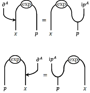
Figure 1: Eigenvalue equations of $q$-exponentials

To get explicit formulas for $q$-exponentials, we best consider the dual pairings between the coordinate algebra of the $q$-deformed position space and that of the corresponding $q$-deformed momentum space [38]:

$$\big{\langle}f(\hskip 0.72229ptp),g(x)\big{\rangle}_{p,\bar{x}} =[\hskip 0.72229ptf(\text{i}^{-1}\partial)\triangleright g(x)]_{x\hskip 0.72229pt=\hskip 0.72229pt0},$$

$$\big{\langle}f(x),g(\hskip 0.72229ptp)\big{\rangle}_{x,\bar{p}} =[\hskip 0.72229ptf(x)\,\bar{\triangleleft}\,g(\partial\hskip 0.72229pt\text{i}^{-1})]_{x\hskip 0.72229pt=\hskip 0.72229pt0}.$$ (148)

Let $\{e^{a}\}$ be a basis of the $q$-deformed position space algebra and let $\{f_{b}\}$ be a dual basis of the corresponding $q$-deformed momentum algebra:

$$\big{\langle}\mathcal{W}_{p}(f_{b}),\mathcal{W}_{x}(e^{a})\big{\rangle}_{p,\bar{x}}=\delta_{b}^{a},\qquad\big{\langle}\mathcal{W}_{x}(e^{a}),\mathcal{W}_{p}(f_{b})\big{\rangle}_{x,\bar{p}}=\delta_{b}^{a},$$ (149)

Now, we are able to write the $q$-exponentials as canonical elements:

$$\exp_{q}(x|\text{i}p) =\sum\nolimits_{a}\mathcal{W}_{x}(e^{a})\otimes\mathcal{W}_{p}(f_{a}),$$

$$\exp_{q}(\text{i}p|x) =\sum\nolimits_{a}\mathcal{W}_{p}(f_{a})\otimes\mathcal{W}_{x}(e^{a}).$$ (150)

The monomials $t^{\hskip 0.72229ptm_{0}}(x^{+})^{m_{+}}(x^{3})^{m_{3}}(x^{-})^{m_{-}}$ form a basis of the commutative coordinate algebra corresponding to the Euclidean quantum space with a time element. We can obtain the elements of the dual basis by the action of the partial derivatives on these monomials. With the help of the operator representations for the partial derivatives in Eqs. (118) and (119) of Chap. 4.2, you can find:

$$\big{\langle}(\text{i}^{-1}E)^{n_{0}}(\text{i}p_{-})^{n_{-}}(\text{i}p_{3})^{n_{3}}(\text{i}p_{+})^{n_{+}},t^{\hskip 0.72229ptm_{0}}(x^{+})^{m_{+}}(x^{3})^{m_{3}}(x^{-})^{m_{-}}\big{\rangle}_{p,\hskip 0.72229pt\bar{x}}=$$

$$=\big{[}(\partial_{0})^{n_{0}}(\partial_{-})^{n_{-}}(\partial_{3})^{n_{3}}(\partial_{+})^{n_{+}}\triangleright t^{\hskip 0.72229ptm_{0}}(x^{+})^{m_{+}}(x^{3})^{m_{3}}(x^{-})^{m_{-}}\big{]}_{x\hskip 0.72229pt=\hskip 0.72229pt0}=$$

$$=\delta_{m_{-},\hskip 0.72229ptn_{-}}\delta_{m_{3},\hskip 0.72229ptn_{3}}\delta_{m_{+},\hskip 0.72229ptn_{+}}\delta_{m_{0},\hskip 0.72229ptn_{0}}\,m_{0}!\,[[\hskip 0.72229ptm_{+}]]_{q^{4}}!\,[[\hskip 0.72229ptm_{3}]]_{q^{2}}!\,[[\hskip 0.72229ptm_{-}]]_{q^{4}}!.$$ (151)

If we calculate dual pairings using right-actions of partial derivatives, we obtain:

$$\big{\langle}t^{\hskip 0.72229ptm_{0}}(x^{+})^{m_{+}}(x^{3})^{m_{3}}(x^{-})^{m_{-}},(\text{i}E)^{n_{0}}(\text{i}^{-1}p_{-})^{n_{-}}(\text{i}^{-1}p_{3})^{n_{3}}(\text{i}^{-1}p_{+})^{n_{+}}\big{\rangle}_{x,\hskip 0.72229pt\bar{p}}=$$

$$\big{[}t^{\hskip 0.72229ptm_{0}}(x^{+})^{m_{+}}(x^{3})^{m_{3}}(x^{-})^{m_{-}}\,\bar{\triangleleft}\,(-\hskip 0.72229pt\partial_{0})^{n_{0}}(-\hskip 0.72229pt\partial_{-})^{n_{-}}(-\hskip 0.72229pt\partial_{3})^{n_{3}}(-\hskip 0.72229pt\partial_{+})^{n_{+}}\big{]}_{x\hskip 0.72229pt=\hskip 0.72229pt0}=$$

$$=\delta_{m_{-},\hskip 0.72229ptn_{-}}\delta_{m_{3},\hskip 0.72229ptn_{3}}\delta_{m_{+},\hskip 0.72229ptn_{+}}\delta_{m_{0},\hskip 0.72229ptn_{0}}\,m_{0}!\,[[\hskip 0.72229ptm_{+}]]_{q^{4}}!\,[[\hskip 0.72229ptm_{3}]]_{q^{2}}!\,[[\hskip 0.72229ptm_{-}]]_{q^{4}}!.$$ (152)

From Eq. (151) or Eq. (152), we can read off the elements being dual to the monomials $t^{\hskip 0.72229ptm_{0}}(x^{+})^{m_{+}}(x^{3})^{m_{3}}(x^{-})^{m_{-}}$. This way, Eq. (150) enables us to write down expressions for $q$-exponentials of the three-dimensional $q$-deformed Euclidean space with a time element. Concretely, we have

$$\exp_{q}(x|\text{i}p) =\exp(\text{i}^{-1}tE)\hskip 0.72229pt\exp_{q}(\mathbf{x}|\text{i}\mathbf{p}),$$

$$\exp_{q}(\text{i}^{-1}p\hskip 0.72229pt|x) =\exp(\text{i}Et)\hskip 0.72229pt\exp_{q}(\text{i}^{-1}\mathbf{p}\hskip 0.72229pt|\mathbf{x}),$$ (153)

with the three-dimensional $q$-exponentials (also see Ref. [12])

$$\exp_{q}(\mathbf{x}|\text{i}\mathbf{p}) =\sum_{\underline{n}\,=\,0}^{\infty}\frac{(q\hskip 0.72229ptx^{+})^{n_{+}}(x^{3})^{n_{3}}(q^{-1}x^{-})^{n_{-}}(\text{i}^{-1}p^{+})^{n_{-}}(\text{i}p^{3})^{n_{3}}(\text{i}^{-1}p^{-})^{n_{+}}}{[[\hskip 0.72229ptn_{+}]]_{q^{4}}!\,[[\hskip 0.72229ptn_{3}]]_{q^{2}}!\,[[\hskip 0.72229ptn_{-}]]_{q^{4}}!},$$

$$\exp_{q}(\text{i}^{-1}\mathbf{p}|\mathbf{x}) =\sum_{\underline{n}\,=\,0}^{\infty}\frac{(\text{i}p^{+})^{n_{+}}(\text{i}^{-1}p^{3})^{n_{3}}(\text{i}p^{-})^{n_{-}}(q^{-1}x^{+})^{n_{-}}(x^{3})^{n_{3}}(q\hskip 0.72229ptx^{-})^{n_{+}}}{[[\hskip 0.72229ptn_{+}]]_{q^{4}}!\,[[\hskip 0.72229ptn_{3}]]_{q^{2}}!\,[[\hskip 0.72229ptn_{-}]]_{q^{4}}}$$ (154)

and the time-dependent phase factors

$$\exp(\text{i}^{-1}t\otimes E)=\sum_{k\hskip 0.72229pt=\hskip 0.72229pt0}^{\infty}\frac{(\text{i}^{-1}t)^{k}\otimes E^{k}}{k!},\qquad\exp(\text{i}E\otimes t)=\sum_{k\hskip 0.72229pt=\hskip 0.72229pt0}^{\infty}\frac{(\text{i}E)^{k}\otimes t^{k}}{k!}.$$ (155)

Note that $E$ is a commutative parameter which we can interpret as energy.

5 Time evolution operator

The $q$-exponentials of the quantum space $\mathcal{\mathbb{R}}_{q}^{3}$ provide us with an operator that generates spatial displacements. We obtain this operator from the expressions for the $q$-exponentials given in Eq. (154) of the previous chapter if we replace the momentum coordinates $p^{A}$ by the derivative operators i${}^{-1}\partial^{A}$ [40, 38, 14]:

$$\exp_{q}(x|\partial_{y})\triangleright g(\hskip 0.72229pty) =g(x\,\bar{\oplus}\,y),$$

$$g(\hskip 0.72229pty)\,\bar{\triangleleft}\,\exp_{q}(-\hskip 0.72229pt\partial_{y}|\hskip 0.72229ptx) =g(\hskip 0.72229pty\,\bar{\oplus}\,x).$$ (156)

We recall that $q$-translations and $q$-inversions are realizations of braided co-products and braided antipodes, respectively [cf. Eqs. (140) and (141) of Chap. 4.4]. The braided co-products and braided antipodes satisfy the axioms (also see Ref. [23])

$$m\circ(\underline{S}\otimes\operatorname*{id})\circ\underline{\Delta} =m\circ(\operatorname*{id}\otimes\,\underline{S}\hskip 0.72229pt)\circ\underline{\Delta}=\underline{\varepsilon},$$

$$m\circ(\underline{\bar{S}}\otimes\operatorname*{id})\circ\underline{\bar{\Delta}} =m\circ(\operatorname*{id}\otimes\,\underline{\bar{S}}\hskip 0.72229pt)\circ\underline{\bar{\Delta}}=\underline{\bar{\varepsilon}},$$ (157)

and

$$(\operatorname*{id}\otimes\,\underline{\varepsilon})\circ\underline{\Delta} =\operatorname*{id}=(\underline{\varepsilon}\otimes\operatorname*{id})\circ\underline{\Delta},$$

$$(\operatorname*{id}\otimes\,\underline{\bar{\varepsilon}})\circ\underline{\bar{\Delta}} =\operatorname*{id}=(\underline{\bar{\varepsilon}}\otimes\operatorname*{id})\circ\underline{\bar{\Delta}}.$$ (158)

In the identities above, we denote the operation of multiplication on the braided Hopf algebra by $m$. The co-units $\underline{\varepsilon},\underline{\bar{\varepsilon}}$ of the two braided Hopf structures are both linear mappings that vanish on the coordinate generators:

$$\varepsilon(X^{i})=\underline{\bar{\varepsilon}}(X^{i})=0.$$ (159)

For this reason, we can realize the co-units $\underline{\varepsilon}$ and $\underline{\bar{\varepsilon}}$ on a commutative coordinate algebra as follows:

$$\underline{\varepsilon}(\mathcal{W}(f))=\underline{\bar{\varepsilon}}(\mathcal{W}(f))=\left.f(x)\right|_{x\hskip 0.72229pt=\hskip 0.72229pt0}=f(0).$$ (160)

Now, we are in a position to translate the Hopf algebra axioms in Eqs. (157) and (158) into corresponding rules for $q$-translations and $q$-inversions [14], i. e.

$$f((\ominus\,x)\oplus x) =f(x\oplus(\ominus\,x))=f(0),$$

$$f((\bar{\ominus}\,x)\,\bar{\oplus}\,x) =f(x\,\bar{\oplus}\,(\bar{\ominus}\,x))=f(0),$$ (161)

and

$$f(x\oplus y)|_{y\hskip 0.72229pt=\hskip 0.72229pt0} =f(x)=f(y\oplus x)|_{y\hskip 0.72229pt=\hskip 0.72229pt0},$$

$$f(x\,\bar{\oplus}\,y)|_{y\hskip 0.72229pt=\hskip 0.72229pt0} =f(x)=f(y\,\bar{\oplus}\,x)|_{y\hskip 0.72229pt=\hskip 0.72229pt0}.$$ (162)

With the help of the rules written down in Eqs. (161) and (162), the identities in Eq. (156) imply

$$\exp_{q}(x\,\bar{\oplus}\,(\bar{\ominus}\,y)|\hskip 0.72229pt\partial_{y})\triangleright g(\hskip 0.72229pty)=g(x\,\bar{\oplus}\,(\bar{\ominus}\,y)\,\bar{\oplus}\,y)=g(x)$$

and

$$[\hskip 0.72229pt\exp_{q}(x|\partial_{y})\triangleright g(\hskip 0.72229pty)]_{\hskip 0.72229pty\hskip 0.72229pt=\hskip 0.72229pt0}=[\hskip 0.72229ptg(x\,\bar{\oplus}\,y)]_{\hskip 0.72229pty\hskip 0.72229pt=\hskip 0.72229pt0}=g(x).$$ (163)

We can combine the above results as follows:

$$\exp_{q}(x\,\bar{\oplus}\,(\bar{\ominus}\,y)|\hskip 0.72229pt\partial_{y})\triangleright g(\hskip 0.72229pty)=[\hskip 0.72229pt\exp_{q}(x|\partial_{y})\triangleright g(\hskip 0.72229pty)]_{\hskip 0.72229pty\hskip 0.72229pt=\hskip 0.72229pt0}=g(x).$$ (164)

Similar identities hold for right-actions:

$$g(\hskip 0.72229pty)\,\bar{\triangleleft}\,\exp_{q}(-\hskip 0.72229pt\partial_{y}|(\bar{\ominus}\,y)\,\bar{\oplus}\,x)=[\hskip 0.72229ptg(y)\,\bar{\triangleleft}\,\exp_{q}(-\hskip 0.72229pt\partial_{y}|\hskip 0.72229ptx)]_{\hskip 0.72229pty\hskip 0.72229pt=\hskip 0.72229pt0}=g(x).$$ (165)

If we apply the results of Eq. (164) or Eq. (165) to the $q$-exponentials given in Eq. (153) of the last chapter, we obtain operators for displacing functions in space and time, i. e.

$$\exp((t-t^{\hskip 0.72229pt\prime})\otimes\partial_{t^{\prime}})\hskip 0.72229pt\exp_{q}(\mathbf{x}\,\bar{\oplus}\,(\bar{\ominus}\,\mathbf{y})|\hskip 0.72229pt\partial_{\mathbf{y}})\triangleright g(\mathbf{y},\hskip 0.72229ptt^{\hskip 0.72229pt\prime})=g(\mathbf{x},t)$$ (166)

or

$$g(\hskip 0.72229pt\mathbf{y},t^{\hskip 0.72229pt\prime})\,\bar{\triangleleft}\,\exp_{q}(-\hskip 0.72229pt\partial_{\mathbf{y}}|(\bar{\ominus}\,\mathbf{y})\,\bar{\oplus}\,\mathbf{x})\hskip 0.72229pt\exp(\partial_{t^{\prime}}\otimes(t^{\hskip 0.72229pt\prime}-t))=g(\mathbf{x},t).$$ (167)

Since the time coordinate is independent of the space coordinates, we can perform time-displacements independently of space-displacements. For this reason, we also have:

$$\exp((t-t^{\hskip 0.72229pt\prime})\otimes\partial_{t^{\prime}})\triangleright g(\mathbf{x},t^{\hskip 0.72229pt\prime}) =[\hskip 0.72229pt\exp(t\otimes\partial_{t^{\prime}})\triangleright g(\mathbf{x},t^{\hskip 0.72229pt\prime})]_{t^{\prime}=\hskip 0.72229pt0}=g(\mathbf{x},t),$$

$$g(\mathbf{x},t^{\hskip 0.72229pt\prime})\triangleleft\exp(\partial_{t^{\prime}}\otimes(t^{\hskip 0.72229pt\prime}-t)) =[\hskip 0.72229ptg(\mathbf{x},\hskip 0.72229ptt^{\hskip 0.72229pt\prime})\triangleleft\hskip 0.72229pt\exp(\partial_{t^{\prime}}\otimes(-\hskip 0.72229ptt))]_{t^{\prime}=\hskip 0.72229pt0}=g(\mathbf{x},t).$$ (168)

In quantum theory, we can calculate the time evolution of a wave function from its values at all points in space at a given time. To see this, we recall the following facts. The time evolution operator is obtained from the operator for a time shift if we replace the time derivative with the Hamilton operator. The Hamilton operator, however, acts on the spatial coordinates, only.

These facts also hold for the $q$-deformed Euclidean space. Let $\phi(\mathbf{x},t)$ be a $q$-deformed wave function describing the quantum state of a system with Hamilton operator $H$. We can calculate $\phi(\mathbf{x},t)$ from $\phi(\mathbf{x},t^{\hskip 0.72229pt\prime}=0)$ using the identities

$$\phi(\mathbf{x},t) =\hskip 0.72229pt\mathcal{U}(t,t^{\hskip 0.72229pt\prime}=0)\triangleright\phi(\mathbf{x},t^{\hskip 0.72229pt\prime}=0),$$

$$\bar{\phi}(\mathbf{x},t) =\bar{\phi}(\mathbf{x},t^{\hskip 0.72229pt\prime}=0)\triangleleft\hskip 0.72229pt\overline{\mathcal{U}}(t,t^{\hskip 0.72229pt\prime}=0)$$ (169)

if the time evolution operators are given by the following expressions:

$$\mathcal{U}(t,t^{\hskip 0.72229pt\prime} =0)=\exp(-\hskip 0.72229ptt\otimes\text{i}H),$$

$$\overline{\mathcal{U}}(t,t^{\hskip 0.72229pt\prime} =0)=\exp(\text{i}H\otimes t).$$ (170)

A look at Eq. (170) shows that the time development operators $\mathcal{U}$ and $\overline{\mathcal{U}}$ of the $q$-deformed Euclidean space have the same form as in the undeformed case. Thus, both time development operators show the same properties as in the undeformed case [41].

We can immediately specify the inverse of both time evolution operators, i. e.

$$\mathcal{U}^{-1}(t,t^{\hskip 0.72229pt\prime}=0)=\hskip 0.72229pt\mathcal{U}(-\hskip 0.72229ptt,t^{\hskip 0.72229pt\prime}=0)=\exp(t\otimes\text{i}H),$$

$$\overline{\mathcal{U}}{}^{-1}(t,t^{\hskip 0.72229pt\prime}=0)=\hskip 0.72229pt\overline{\mathcal{U}}(-\hskip 0.72229ptt,t^{\hskip 0.72229pt\prime}=0)=\exp(-\text{i}H\otimes t),$$ (171)

with

$$\mathcal{U}(t,t^{\hskip 0.72229pt\prime}=0)\,\mathcal{U}^{-1}(t,t^{\hskip 0.72229pt\prime}=0)=\,\, \mathcal{U}^{-1}(t,t^{\hskip 0.72229pt\prime}=0)\,\mathcal{U}(t,t^{\hskip 0.72229pt\prime}=0)=1,$$

$$\overline{\mathcal{U}}{}^{-1}(t,t^{\hskip 0.72229pt\prime}=0)\,\overline{\mathcal{U}}(t,t^{\hskip 0.72229pt\prime}=0)=\,\, \overline{\mathcal{U}}(t,t^{\hskip 0.72229pt\prime}=0)\,\overline{\mathcal{U}}{}^{-1}(t,t^{\hskip 0.72229pt\prime}=0)=1.$$ (172)

The inverse of each time evolution operator transforms wave functions into the opposite time direction:

$$\phi(\mathbf{x},-\hskip 0.72229ptt) =\hskip 0.72229pt\mathcal{U}^{-1}(t,t^{\hskip 0.72229pt\prime}=0)\triangleright\phi(\mathbf{x},t^{\hskip 0.72229pt\prime}=0),$$

$$\bar{\phi}(\mathbf{x},-\hskip 0.72229ptt) =\bar{\phi}(\mathbf{x},t^{\hskip 0.72229pt\prime}=0)\triangleleft\,\overline{\mathcal{U}}{}^{-1}(t,t^{\hskip 0.72229pt\prime}=0).$$ (173)

If we apply the inverse time evolution operators to Eq. (169) and take into account Eq. (172), we also get:

$$\phi(\mathbf{x},t^{\hskip 0.72229pt\prime} =0)=\hskip 0.72229pt\mathcal{U}^{-1}(t,t^{\hskip 0.72229pt\prime}=0)\triangleright\phi(\mathbf{x},t),$$

$$\bar{\phi}(\mathbf{x},t^{\hskip 0.72229pt\prime} =0)=\bar{\phi}(\mathbf{x},t)\triangleleft\,\overline{\mathcal{U}}{}^{-1}(t,t^{\hskip 0.72229pt\prime}=0).$$ (174)

The time evolution operators in Eq. (170) shift the wave functions from the time-zero point. We can eliminate this restriction by generalizing the time evolution operators in the following way:

$$\mathcal{U}(t,t^{\hskip 0.72229pt\prime}) =\hskip 0.72229pt\mathcal{U}(t,t^{\hskip 0.72229pt\prime\prime}=0)\,\mathcal{U}^{-1}(t^{\hskip 0.72229pt\prime},t^{\hskip 0.72229pt\prime\prime}=0)=\exp(-(t-t^{\hskip 0.72229pt\prime})\otimes\text{i}H),$$

$$\overline{\mathcal{U}}(t,t^{\hskip 0.72229pt\prime}) =\hskip 0.72229pt\overline{\mathcal{U}}{}^{-1}(t^{\hskip 0.72229pt\prime},t^{\hskip 0.72229pt\prime\prime}=0)\,\overline{\mathcal{U}}(t,t^{\hskip 0.72229pt\prime\prime}=0)=\exp(-\text{i}H\otimes(t^{\hskip 0.72229pt\prime}-t)).$$ (175)

Applying Eqs. (169), (174), and (175), we can see that the operators above transform wave functions from time $t^{\hskip 0.72229pt\prime}$ to time $t$:

$$\phi(\mathbf{x},t) =\hskip 0.72229pt\mathcal{U}(t,t^{\hskip 0.72229pt\prime})\triangleright\phi(\mathbf{x},t^{\hskip 0.72229pt\prime}),$$

$$\bar{\phi}(\mathbf{x},t) =\bar{\phi}(\mathbf{x},t^{\hskip 0.72229pt\prime})\triangleleft\,\overline{\mathcal{U}}(t,t^{\hskip 0.72229pt\prime}).$$ (176)

The general time evolution operators in Eq. (175) have an inverse again, i. e. there are operators $\mathcal{U}^{-1}(t,t^{\hskip 0.72229pt\prime})$ and $\overline{\mathcal{U}}{}^{-1}(t,t^{\hskip 0.72229pt\prime})$ with

$$\mathcal{U}(t,t^{\hskip 0.72229pt\prime})\,\mathcal{U}^{-1}(t,t^{\hskip 0.72229pt\prime}) =\hskip 0.72229pt\mathcal{U}^{-1}(t,t^{\hskip 0.72229pt\prime})\,\mathcal{U}(t,t^{\hskip 0.72229pt\prime})=1,$$

$$\overline{\mathcal{U}}(t,t^{\hskip 0.72229pt\prime})\,\overline{\mathcal{U}}{}^{-1}(t,t^{\hskip 0.72229pt\prime}) =\hskip 0.72229pt\overline{\mathcal{U}}{}^{-1}(t,t^{\hskip 0.72229pt\prime})\,\overline{\mathcal{U}}(t,t^{\hskip 0.72229pt\prime})=1.$$ (177)

These identities are satisfied by the following expressions:

$$\mathcal{U}^{-1}(t,t^{\hskip 0.72229pt\prime}) =\hskip 0.72229pt\mathcal{U}(t^{\hskip 0.72229pt\prime},t^{\hskip 0.72229pt\prime\prime}=0)\,\mathcal{U}^{-1}(t,t^{\hskip 0.72229pt\prime\prime}=0)=\hskip 0.72229pt\mathcal{U}(t^{\hskip 0.72229pt\prime},t)$$

$$=\hskip 0.72229pt\mathcal{U}(-\hskip 0.72229ptt,-\hskip 0.72229ptt^{\prime})=\exp((t-t^{\hskip 0.72229pt\prime})\otimes\text{i}H),$$ (178)

$$\overline{\mathcal{U}}{}^{-1}(t,t^{\hskip 0.72229pt\prime}) =\hskip 0.72229pt\overline{\mathcal{U}}{}^{-1}(t,t^{\hskip 0.72229pt\prime\prime}=0)\,\overline{\mathcal{U}}(t^{\hskip 0.72229pt\prime},t^{\hskip 0.72229pt\prime\prime}=0)=\hskip 0.72229pt\overline{\mathcal{U}}(t^{\hskip 0.72229pt\prime},t)$$

$$=\hskip 0.72229pt\overline{\mathcal{U}}(-\hskip 0.72229ptt,-\hskip 0.72229ptt^{\hskip 0.72229pt\prime})=\exp(\text{i}H\otimes(t^{\hskip 0.72229pt\prime}-t)).$$ (179)

The operator $\mathcal{U}(t,t^{\hskip 0.72229pt\prime})$ describes the evolution from time $t^{\hskip 0.72229pt\prime}$ to time $t$, and the inverse operator $\mathcal{U}^{-1}(t,t^{\hskip 0.72229pt\prime})$ turns around this evolution. The same holds for the operators $\overline{\mathcal{U}}(t,t^{\hskip 0.72229pt\prime})$ and $\overline{\mathcal{U}}{}^{-1}(t,t^{\hskip 0.72229pt\prime})$. Thus, we have in analogy to Eq. (176):

$$\phi(\mathbf{x},t^{\hskip 0.72229pt\prime}) =\hskip 0.72229pt\mathcal{U}^{-1}(t,t^{\hskip 0.72229pt\prime})\triangleright\phi(\mathbf{x},t),$$

$$\bar{\phi}(\mathbf{x},t^{\hskip 0.72229pt\prime}) =\bar{\phi}(\mathbf{x},t)\triangleleft\,\overline{\mathcal{U}}{}^{-1}(t,t^{\hskip 0.72229pt\prime}).$$ (180)

The time evolution operators defined in Eq. (175) satisfy the principle of causality. Accordingly, we can write the successive action of two different time evolution operators as the action of one single time evolution operator. Concretely, we have

$$\mathcal{U}(t,t^{\hskip 0.72229pt\prime\prime})\,\mathcal{U}(t^{\hskip 0.72229pt\prime\prime},t^{\hskip 0.72229pt\prime}) =\hskip 0.72229pt\mathcal{U}(t,0)\,\mathcal{U}^{-1}(t^{\hskip 0.72229pt\prime\prime},0)\,\mathcal{U}(t^{\hskip 0.72229pt\prime\prime},0)\,\mathcal{U}^{-1}(t^{\hskip 0.72229pt\prime},0)$$

$$=\hskip 0.72229pt\mathcal{U}(t,0)\,\mathcal{U}^{-1}(t^{\hskip 0.72229pt\prime},0)=\hskip 0.72229pt\mathcal{U}(t,t^{\hskip 0.72229pt\prime})$$ (181)

and

$$\overline{\mathcal{U}}(t^{\hskip 0.72229pt\prime\prime},t^{\hskip 0.72229pt\prime})\,\overline{\mathcal{U}}(t,t^{\hskip 0.72229pt\prime\prime}) =\hskip 0.72229pt\overline{\mathcal{U}}{}^{-1}(t^{\hskip 0.72229pt\prime},0)\,\overline{\mathcal{U}}(t^{\hskip 0.72229pt\prime\prime},0)\,\overline{\mathcal{U}}{}^{-1}(t^{\hskip 0.72229pt\prime\prime},0)\,\overline{\mathcal{U}}(t,0)$$

$$=\hskip 0.72229pt\overline{\mathcal{U}}{}^{-1}(t^{\hskip 0.72229pt\prime},0)\,\overline{\mathcal{U}}(t,0)=\hskip 0.72229pt\overline{\mathcal{U}}(t,t^{\hskip 0.72229pt\prime}).$$ (182)

Recall that the time element has trivial braiding properties and that the Hamilton operator acts on the space coordinates, only. For this reason, the Hamilton operator commutes with the time variable, and we can drop the symbol for the tensor product in the expressions for the time evolution operator:

$$\exp(t\otimes\text{i}H)=\exp(\text{i}H\otimes t)=\exp(\text{i}Ht).$$ (183)

Accordingly, we can also write:

$$\mathcal{U}(t,t^{\hskip 0.72229pt\prime})=\exp(-\text{i}H(t-t^{\hskip 0.72229pt\prime})),\qquad\overline{\mathcal{U}}(t,t^{\hskip 0.72229pt\prime})=\exp(\text{i}H(t-t^{\hskip 0.72229pt\prime})).$$ (184)

With this result we can make the following identifications:

$$\mathcal{U}(t,t^{\hskip 0.72229pt\prime})=\hskip 0.72229pt\overline{\mathcal{U}}(-\hskip 0.72229ptt,-\hskip 0.72229ptt^{\hskip 0.72229pt\prime})=\hskip 0.72229pt\mathcal{U}^{-1}(-\hskip 0.72229ptt,-\hskip 0.72229ptt^{\hskip 0.72229pt\prime})=\hskip 0.72229pt\overline{\mathcal{U}}{}^{-1}(t,t^{\hskip 0.72229pt\prime}).$$ (185)

From Eq. (184) also follows that the time evolution operators are unitary since the Hamilton operator is Hermitian:

$$\mathcal{U}^{-1}(t,t^{\hskip 0.72229pt\prime})=\hskip 0.72229pt\mathcal{U}(t^{\hskip 0.72229pt\prime},t)=\hskip 0.72229pt\overline{\mathcal{U}}(t,t^{\hskip 0.72229pt\prime})=\hskip 0.72229pt\mathcal{U}^{{\dagger}}(t,t^{\hskip 0.72229pt\prime}).$$ (186)

6 Schrödinger picture and Heisenberg picture

As explained in the last chapter, the time evolution operator of the three-dimensional $q$-deformed Euclidean space takes on the same form as in the undeformed case. This fact enables us to apply the well-known methods for describing the time evolution of a quantum mechanical system to the three-dimensional $q$-deformed Euclidean space.

First, we derive a differential equation for the time evolution operator $\mathcal{U}(t,t^{\hskip 0.72229pt\prime})$:

$$\partial_{t}\triangleright\mathcal{U}(t,t^{\hskip 0.72229pt\prime}) =\partial_{t}\triangleright\mathcal{U}(t,0)\,\mathcal{U}^{-1}(t^{\hskip 0.72229pt\prime},0)=\partial_{t}\triangleright\exp(-\hskip 0.72229ptt\otimes\text{i}H)\,\mathcal{U}^{-1}(t^{\hskip 0.72229pt\prime},0)$$

$$=\exp(-\hskip 0.72229ptt\otimes\text{i}H)\hskip 0.72229pt(-\text{i}H)\,\mathcal{U}^{-1}(t^{\hskip 0.72229pt\prime},0)=-\text{i}H\,\mathcal{U}(t,0)\,\mathcal{U}^{-1}(t^{\hskip 0.72229pt\prime},0)$$

$$=-\text{i}H\,\mathcal{U}(t,t^{\hskip 0.72229pt\prime}).$$ (187)

In the above calculation, we have made use of Eqs. (170) and (175) of the previous chapter. We can proceed in the same way for the time evolution operator corresponding to right-actions:

$$\overline{\mathcal{U}}(t,t^{\hskip 0.72229pt\prime})\triangleleft\partial_{t} =\hskip 0.72229pt\overline{\mathcal{U}}{}^{-1}(t^{\hskip 0.72229pt\prime},0)\,\overline{\mathcal{U}}(t,0)\triangleleft\partial_{t}=\hskip 0.72229pt\overline{\mathcal{U}}{}^{-1}(t^{\hskip 0.72229pt\prime},0)\hskip 0.72229pt\exp(\text{i}H\otimes t)\triangleleft\partial_{t}$$

$$=\hskip 0.72229pt\overline{\mathcal{U}}{}^{-1}(t^{\hskip 0.72229pt\prime},0)\hskip 0.72229pt(-\text{i}H)\hskip 0.72229pt\exp(\text{i}H\otimes t)=\hskip 0.72229pt\overline{\mathcal{U}}{}^{-1}(t^{\hskip 0.72229pt\prime},0)\,\overline{\mathcal{U}}(t,0)\hskip 0.72229pt(-\text{i}H)$$

$$=\hskip 0.72229pt\overline{\mathcal{U}}(t,t^{\hskip 0.72229pt\prime})\hskip 0.72229pt(-\text{i}H).$$ (188)

The calculations in Eqs. (187) and (188) lead us to the so-called Schrödinger equations of the time evolution operators. If we take into account that the operator representations of $\partial_{0}$ and $\hat{\partial}_{0}$ are nothing else but the usual time derivative [cf. Eqs. (119) and (123) of Chap. 4.2], we can write these Schrödinger equations as follows:

$$\text{i}\partial_{0}\triangleright\mathcal{U}(t,t^{\hskip 0.72229pt\prime}) =H\,\mathcal{U}(t,t^{\hskip 0.72229pt\prime}), \mathcal{U}(t^{\hskip 0.72229pt\prime},t)\,\bar{\triangleleft}\,\partial_{0}\text{i} =\mathcal{U}(t^{\hskip 0.72229pt\prime},t)\hskip 0.72229ptH,$$

$$\text{i}\hat{\partial}_{0}\,\bar{\triangleright}\,\hskip 0.72229pt\mathcal{\hat{U}}(t,t^{\hskip 0.72229pt\prime}) =\hat{H}\,\mathcal{\hat{U}}(t,t^{\hskip 0.72229pt\prime}), \mathcal{\hat{U}}(t^{\hskip 0.72229pt\prime},t)\triangleleft\hat{\partial}_{0}\text{i} =\mathcal{\hat{U}}(t^{\hskip 0.72229pt\prime},t)\hskip 0.72229pt\hat{H}.$$ (189)

Note that the Hamilton operators $H$ and $\hat{H}$ depend on $\partial^{A}$ and $\hat{\partial}^{A}$, respectively [also see Eqs. (118) and (122) of Chap. 4.2].

The two Schrödinger equations of $\mathcal{U}$ have their equivalent in the integral equations

$$\mathcal{U}(t,t^{\hskip 0.72229pt\prime}) =1-\text{i}\int\nolimits_{t^{\prime}}^{t}\text{d}t^{\hskip 0.72229pt\prime\prime}\,H(t^{\hskip 0.72229pt\prime\prime})\,\mathcal{U}(t^{\hskip 0.72229pt\prime\prime},t^{\hskip 0.72229pt\prime}),$$

$$\mathcal{U}(t^{\hskip 0.72229pt\prime},t) =1+\text{i}\int\nolimits_{t^{\prime}}^{t}\text{d}t^{\hskip 0.72229pt\prime\prime}\,\mathcal{U}(t^{\hskip 0.72229pt\prime},t^{\hskip 0.72229pt\prime\prime})\,H(t^{\hskip 0.72229pt\prime\prime})$$ (190)

if we assume the following constraint:

$$\mathcal{U}(t,t)=1.$$ (191)

The above integral equations have formal solutions

$$\mathcal{U}(t,t^{\hskip 0.72229pt\prime})=1+\sum_{n\hskip 0.72229pt=\hskip 0.72229pt1}^{\infty}\text{i}^{-n}\int\limits_{t^{\prime}}^{t}\text{d}t_{1}\int\limits_{t^{\prime}}^{t_{1}}\text{d}t_{2}\hskip 0.72229pt\ldots\int\limits_{t^{\prime}}^{t_{n-1}}\text{d}t_{n}\,H(t_{1})\hskip 0.72229ptH(t_{2})\ldots\hskip 0.72229ptH(t_{n})$$ (192)

and

$$\mathcal{U}(t^{\hskip 0.72229pt\prime},t)=1+\sum_{n\hskip 0.72229pt=\hskip 0.72229pt1}^{\infty}\text{i}^{n}\int\limits_{t^{\prime}}^{t}\text{d}t_{1}\int\limits_{t^{\prime}}^{t_{1}}\text{d}t_{2}\hskip 0.72229pt\ldots\int\limits_{t^{\prime}}^{t_{n-1}}\text{d}t_{n}\,H(t_{n})\hskip 0.72229ptH(t_{n-1})\ldots\hskip 0.72229ptH(t_{1}).$$

For the operators $\mathcal{\hat{U}}$ and $\hat{H}$, similar formulas apply, which we obtain by replacing $\mathcal{U}$ and $H$ with $\mathcal{\hat{U}}$ and $\hat{H}$, respectively.

In quantum theory, there are two ways of describing the time evolution of a quantum system, namely the Schrödinger picture and the Heisenberg picture. In the Schrödinger picture, the time evolution is determined by the time dependence of the wave functions, whereas the observables are usually independent of time. We can derive the equations of motion for the wave functions by using Eqs. (176) and (189):

$$\text{i}\partial_{0}\triangleright\phi(\mathbf{x},t) =\text{i}\partial_{t}\triangleright\mathcal{U}(t,t^{\hskip 0.72229pt\prime})\triangleright\phi(\mathbf{x},t^{\hskip 0.72229pt\prime})$$

$$=H\,\mathcal{U}(t,t^{\hskip 0.72229pt\prime})\triangleright\phi(\mathbf{x},t^{\hskip 0.72229pt\prime})=H\triangleright\phi(\mathbf{x},t).$$ (193)

Similarly, we get:

$$\phi(\mathbf{x},t)\triangleleft\hat{\partial}_{0}\text{i} =\phi(\mathbf{x},t^{\hskip 0.72229pt\prime})\triangleleft\hskip 0.72229pt\mathcal{\hat{U}}(t^{\hskip 0.72229pt\prime},t)\triangleleft\partial_{t}\text{i}$$

$$=\phi(\mathbf{x},t^{\hskip 0.72229pt\prime})\triangleleft\hskip 0.72229pt\mathcal{\hat{U}}(t^{\hskip 0.72229pt\prime},t)\hskip 0.72229pt\hat{H}=\phi(\mathbf{x},t)\triangleleft\hat{H}.$$ (194)

We obtain further equations of motion by applying the following substitution to the above identities:

$$\partial_{0}\leftrightarrow\hat{\partial}_{0},\qquad\mathcal{U}\leftrightarrow\mathcal{\hat{U}},\qquad H\leftrightarrow\hat{H},\qquad\triangleright\leftrightarrow\bar{\triangleright},\qquad\triangleleft\leftrightarrow\bar{\triangleleft}.$$ (195)

Due to these substitution rules, we will restrict ourselves to the time development operator $\mathcal{U}$ and the Hamilton operator $H$.

We show in the appendix that the following expression defines a $q$-deformed scalar product of two time-dependent wave functions:

$$\big{\langle}\phi(t)|\hskip 0.72229pt\psi(t)\big{\rangle}_{q}=\int\text{d}_{q}^{3}x\,\overline{\phi(\mathbf{x},t)}\circledast\psi(\mathbf{x},t).$$ (196)

The time dependence of the scalar product results from the wave functions only. We now show that the above scalar product does not change in time if the time development operator is unitary:

$$\big{\langle}\phi(t)|\hskip 0.72229pt\psi(t)\big{\rangle}_{q} =\int\text{d}_{q}^{3}x\,\overline{\phi(\mathbf{x},t)}\circledast\psi(\mathbf{x},t)$$

$$=\int\text{d}_{q}^{3}x\,[\hskip 0.72229pt\overline{\phi(x,0)}\triangleleft\mathcal{U}^{{\dagger}}(t,0)]\circledast[\,\mathcal{U}(t,0)\triangleright\psi(\mathbf{x},0)]$$

$$=\int\text{d}_{q}^{3}x\,\overline{\phi(\mathbf{x},0)}\circledast[\,\mathcal{U}^{-1}(t,0)\,\mathcal{U}(t,0)\triangleright\psi(\mathbf{x},0)]$$

$$=\int\text{d}_{q}^{3}x\,\overline{\phi(\mathbf{x},0)}\circledast\psi(\mathbf{x},0)=\big{\langle}\phi(0)|\hskip 0.72229pt\psi(0)\big{\rangle}_{q}.$$ (197)

In the above calculation, we made use of Eqs. (169) and (186) of the previous chapter. In addition to this, we took into account that the operators $\mathcal{U}(t,0)$ and $\mathcal{U}^{-1}(t,0)$ depend on the partial derivatives $\partial^{A}$ for which we have the following $q$-analog of Stokes’ theorem [14]:

$$\int_{-\infty}^{+\infty}\text{d}_{q}^{3}x\,(f\triangleleft\partial^{A})\circledast g=\int_{-\infty}^{+\infty}\text{d}_{q}^{3}x\,f\circledast(\partial^{A}\triangleright g).$$ (198)

The result of Eq. (197) implies that the normalization of a wave function does not change over time:

$$\big{\langle}\phi(t)|\hskip 0.72229pt\phi(t)\big{\rangle}_{q}=1.$$ (199)

Next, we examine the time dependence of matrix elements of an observable, which in the following is denoted by $\hat{O}$. With similar considerations as in Eq. (197), we get:

$$\big{\langle}\phi(t)|\hskip 0.72229pt\hat{O}\triangleright\psi(t)\big{\rangle}_{q} =\int\text{d}_{q}^{3}x\,\overline{\phi(\mathbf{x},t)}\circledast(\hat{O}\triangleright\psi(\mathbf{x},t))$$

$$=\int\text{d}_{q}^{3}x\hskip 2.168pt[\hskip 0.72229pt\overline{\phi(x,0)}\triangleleft\mathcal{U}^{{\dagger}}(t,0)]\circledast[\hat{O}\,\mathcal{U}(t,0)\triangleright\psi(\mathbf{x},0)]$$

$$=\int\text{d}_{q}^{3}x\,\overline{\phi(\mathbf{x},0)}\circledast[\,\mathcal{U}^{-1}(t,0)\hskip 0.72229pt\hat{O}\,\mathcal{U}(t,0)\triangleright\psi(\mathbf{x},0)].$$ (200)

From the above result, we can read off an expression for observables of the Heisenberg picture:

$$\hat{O}_{H}=\hskip 0.72229pt\mathcal{U}^{-1}(t,0)\hskip 0.72229pt\hat{O}\,\mathcal{U}(t,0)=\hskip 0.72229pt\mathcal{U}(0,t)\hskip 0.72229pt\hat{O}\,\mathcal{U}^{-1}(0,t).$$ (201)

Note that the second expression is a consequence of Eq. (186) in the previous chapter. A look at Eq. (200) also shows that the wave function of the Heisenberg picture does not depend on time:

$$\phi_{H}(\mathbf{x})=\phi(\mathbf{x},t=0).$$ (202)

With these conventions, the Heisenberg picture yields the same matrix elements as the Schrödinger picture:

$$\big{\langle}\phi|\hat{O}\triangleright\psi\big{\rangle}_{q} =\int\text{d}_{q}^{3}x\,\overline{\phi(\mathbf{x},t)}\circledast\hat{O}\triangleright\psi(\mathbf{x},t)$$

$$=\int\text{d}_{q}^{3}x\,\overline{\phi(\mathbf{x})}\circledast\hat{O}_{H}\triangleright\psi_{H}(\mathbf{x})=\big{\langle}\phi_{H}|\hskip 0.72229pt\hat{O}_{H}\triangleright\psi_{H}\big{\rangle}_{q}.$$ (203)

As is well-known, the observables of the Heisenberg picture fulfill the so-called Heisenberg equations of motion. If the Hamilton operator shows no explicit time-dependence, it holds in complete analogy to the undeformed case [42]:

$$\frac{\text{d}\hat{O}_{H}}{\text{d}t} =\frac{\partial\hskip 0.72229pt\mathcal{U}^{-1}(t,0)}{\partial\hskip 0.72229ptt}\,\hat{O}\,\mathcal{U}(t,0)+\hskip 0.72229pt\mathcal{U}^{-1}(t,0)\,\hat{O}\,\frac{\partial\hskip 0.72229pt\mathcal{U}(t,0)}{\partial\hskip 0.72229ptt}$$

$$=\text{i}H\,\mathcal{U}^{-1}(t,0)\hskip 0.72229pt\hat{O}\,\mathcal{U}(t,0)-\hskip 0.72229pt\mathcal{U}^{-1}(t,0)\hskip 0.72229pt\hat{O}\,\mathcal{U}(t,0)\,\text{i}H$$

$$=\text{i}[H,\hat{O}_{H}],$$ (204)

$$\frac{\text{d}\hat{O}_{H}}{\text{d}t} =\frac{\partial\hskip 0.72229pt\mathcal{U}(0,t)}{\partial\hskip 0.72229ptt}\,\hat{O}\,\mathcal{U}^{-1}(0,t)+\hskip 0.72229pt\mathcal{U}(0,t)\,\hat{O}\,\frac{\partial\hskip 0.72229pt\mathcal{U}^{-1}(0,t)}{\partial\hskip 0.72229ptt}$$

$$=\text{i}H\,\mathcal{U}(0,t)\hskip 0.72229pt\hat{O}\,\mathcal{U}^{-1}(0,t)-\hskip 0.72229pt\mathcal{U}(0,t)\hskip 0.72229pt\hat{O}\,\mathcal{U}^{-1}(0,t)\,\text{i}H$$

$$=\text{i}[H,\hat{O}_{H}].$$ (205)

Note that we have to add $\partial\hat{O}_{H}/\partial t$ on the right-hand side of the above equations of motion if $\hat{O}$ shows an explicit time dependence.

Appendix A Scalar product for the $q$-deformed Euclidean space

In the following, we show that the expression

$$\big{\langle}f|\hskip 0.72229ptg\big{\rangle}_{q}=\int\text{d}_{q}^{3}x\,\overline{f(\mathbf{x})}\circledast g(\mathbf{x})$$ (206)

has all the properties of a scalar product.

Recall that the star-product is distributive, and the $q$-integral over the Euclidean quantum space is linear. Therefore, the expression in Eq. (206) is antilinear in its first argument, and it is linear in its second argument:

$$\left\langle f|\hskip 0.72229ptg_{1}+g_{2}\right\rangle_{q} =\left\langle f|\hskip 0.72229ptg_{1}\right\rangle_{q}+\left\langle f|\hskip 0.72229ptg_{2}\right\rangle_{q}, \left\langle f|\alpha\hskip 0.72229ptg\right\rangle_{q} =\alpha\left\langle f|\hskip 0.72229ptg\right\rangle_{q},$$

$$\left\langle f_{1}+f_{2}|\hskip 0.72229ptg\right\rangle_{q} =\left\langle f_{1}|\hskip 0.72229ptg\right\rangle_{q}+\left\langle f_{2}|\hskip 0.72229ptg\right\rangle_{q}, \left\langle\alpha\hskip 0.72229ptf|g\right\rangle_{q} =\bar{\alpha}\left\langle f|\hskip 0.72229ptg\right\rangle_{q}.$$ (207)

Note that $\alpha$ is a complex number with $\bar{\alpha}$ being its complex conjugate. Due to the identities of Eq. (207), the expression in Eq. (206) is a so-called sesquilinear form.

It follows from the conjugation properties of star-product and $q$-integral [cf. Eq. (114) of Chap. 4.1 and Eq. (133) of Chap. 4.3] that the bilinear form in Eq. (206) is also conjugate-symmetrical:

$$\overline{\left\langle f|\hskip 0.72229ptg\right\rangle} =\overline{\int\text{d}_{q}^{3}x\,\overline{f(\mathbf{x})}\circledast g(\mathbf{x})}=\int\text{d}_{q}^{3}x\,\overline{\overline{f(\mathbf{x})}\circledast g(\mathbf{x})}$$

$$=\int\text{d}_{q}^{3}x\,\overline{g(\mathbf{x})}\circledast f(\mathbf{x})=\left\langle g|f\right\rangle.$$ (208)

Next, we prove that the bilinear form in Eq. (206) is positive definite for all $q\$from a neighborhood of $1$ [43]. To this end, we first show that there can be no function $f_{q}$ other than the zero function fulfilling the following condition:

$$\big{\langle}f_{q}|f_{q}\big{\rangle}_{q}=\int_{-\infty}^{+\infty}\text{d}_{q}^{3}x\,\overline{f_{q}(\mathbf{x})}\circledast f_{q}(\mathbf{x})=0.$$ (209)

We assume that $f_{q}$ is a function subject to the above identity. Moreover, we can assume that $f_{q}$ depends continuously on the deformation parameter $q$. For this reason, we write $f_{q}$ as

$$f_{q}(\mathbf{x})=\sum_{k\hskip 0.72229pt=\hskip 0.72229pt0}^{\infty}\hskip 0.72229ptf_{q,k}(\mathbf{x})\hskip 0.72229pt(q-1)^{k}$$ (210)

with $f_{q,k}(\mathbf{x})$ showing the following property:

$$\lim_{q\hskip 0.72229pt\rightarrow 1}f_{q,k}(\mathbf{x})=f_{1,k}(\mathbf{x})=0\qquad\Rightarrow\qquad f_{q,k}(\mathbf{x})=0.$$ (211)

The condition in Eq. (211) guarantees that $f_{q,k}$ does not vanish for $q=1$ unless $f_{q,k}$ is identical to the zero function for any value of $q$ from a neighborhood of $1$.

The bilinear form in Eq. (206) becomes the usual scalar product in the limiting case $q=1$. For this reason, we have:

$$0=\lim_{q\hskip 0.72229pt\rightarrow 1}\int_{-\infty}^{+\infty}\text{d}_{q}^{3}x\,\overline{f_{q}(\mathbf{x})}\circledast f_{q}(\mathbf{x})=\int_{-\infty}^{+\infty}\text{d}^{3}x\,\overline{f_{1,0}(\mathbf{x})}\cdot f_{1,0}(\mathbf{x}).$$ (212)

Since the ordinary scalar product on the right side of Eq. (212) is positive definite, it holds $f_{1,0}=0$ and, because of Eq. (211), we also have $f_{q,0}=0$. Next, we insert the expansion of Eq. (210) into the expression of Eq. (209):

$$0 =\int_{-\infty}^{+\infty}\text{d}_{q}^{3}x\sum_{k,l\hskip 0.72229pt=\hskip 0.72229pt1}^{\infty}\,\overline{f_{q,k}(\mathbf{x})}\circledast f_{q,l}(\mathbf{x})\,(q-1)^{k\hskip 0.72229pt+\hskip 0.72229ptl}$$

$$=(q-1)^{2}\int_{-\infty}^{+\infty}\text{d}_{q}^{3}x\,\overline{f_{q,1}(\mathbf{x})}\circledast f_{q,1}(\mathbf{x})+O((q-1)^{3}).$$ (213)

This way, we get:

$$\int_{-\infty}^{+\infty}\text{d}_{q}^{3}x\,\overline{f_{q,1}(\mathbf{x})}\circledast f_{q,1}(\mathbf{x})=O(q-1).$$ (214)

Accordingly, the integral on the left-hand side of the above equation must vanish in the limiting case $q\rightarrow 1$:

$$0=\lim_{q\hskip 0.72229pt\rightarrow 1}\int_{-\infty}^{+\infty}\text{d}_{q}^{3}x\,\overline{f_{q,1}(\mathbf{x})}\circledast f_{q,1}(\mathbf{x})=\int_{-\infty}^{+\infty}\text{d}^{3}x\,\overline{f_{1,1}(\mathbf{x})}\cdot f_{1,1}(\mathbf{x}).$$ (215)

From the positive definiteness of the ordinary scalar product follows $f_{1,1}=0$. Due to Eq. (211), this implies that $f_{q,1}$ is also identical to the zero function. We can repeat this argument for all $f_{q,k}$ with $k\geq 2$, one after the other. Thus, we have $f_{q,k}=0$ for all $k\in\mathbb{N}_{0}$. Therefore $f_{q}=0$ is valid. In other words, no function different from the zero function satisfies the identity in Eq. (209):

$$\big{\langle}f_{q}|f_{q}\big{\rangle}_{q}=0\quad\Leftrightarrow\quad f_{q}=0.$$ (216)

Now we are ready to complete the proof that the bilinear form in Eq. (206) is positive definite for all $q$ from a neighborhood of $1$, i. e.

$$\big{\langle}f|f\big{\rangle}_{q}>0\quad\text{for}\quad f\neq 0.$$ (217)

In the following, $B(1)$ is a neighborhood of $1$, so that Eq. (216) is satisfied for all $q\in B(1)$. We assume that there is a $q^{\ast}\in B(1)$ and a function $f\neq 0$ such that

$$\big{\langle}f|f\big{\rangle}_{q^{\ast}}<0.$$ (218)

This assumption together with

$$\lim_{q\hskip 0.72229pt\rightarrow 1}\big{\langle}f|f\big{\rangle}_{q} =\lim_{q\hskip 0.72229pt\rightarrow 1}\int_{-\infty}^{+\infty}\text{d}_{q}^{3}x\,\overline{f_{q}(\mathbf{x})}\circledast f_{q}(\mathbf{x})$$

$$=\int_{-\infty}^{+\infty}\text{d}^{3}x\,\overline{f(\mathbf{x})}\cdot f(\mathbf{x})=\big{\langle}f|f\big{\rangle}>0$$ (219)

implies that a $q^{\ast\ast}\in B(1)$ exists with

$$\big{\langle}f|f\big{\rangle}_{q^{\ast\ast}}=0.$$ (220)

However, this conclusion contradicts Eq. (216) due to $f\neq 0$, i. e. Eq. (217) must apply to all $q\in B(1)$.

References

- [1] L. J. Garay. Quantum gravity and minimum length. Int. J. Phys. A, 10:145–165, 1995.
- [2] A. Hagar. Discrete or Continuous? The Quest for Fundamental Length in Modern Physics. Cambridge University Press, Cambridge/UK, 2014.
- [3] W. Heisenberg. Die Selbstenergie des Elektrons. Z. Phys., 64:4–63, 1930.
- [4] W. Heisenberg. Die Grenzen der Anwendbarkeit der bisherigen Quantentheorie. Z. Phys., 110:241–266, 1938.
- [5] C. A. Mead. Observable consequences of fundamental-length hypotheses. Phys. Rev., 143:990–1005, 1966.
- [6] M. Fichtmüller, A. Lorek, and J. Wess. -deformed phase space and its lattice structure. Z. Phys. C, 71(3):533–537, 1996.
- [7] A. Lorek, W. Weich, and J. Wess. Non-commutative Euclidean and Minkowski structures. Z. Phys. C, 76:375–386, 1997.
- [8] H. Wachter. Momentum and position representations for the -deformed euclidean space. 2019. arXiv:math-ph/1910.02283.
- [9] U. Carow-Watamura, M. Schlieker, M. Scholl, and S. Watamura. Tensor representation of the quantum group SLq(2,C) and quantum Minkowski space. Z. Phys. C, 48:159–166, 1990.
- [10] A. Lorek, W. B. Schmidke, and J. Wess. SU-covariant R-matrices for reducible representations. Lett. Math. Phys., 31:279–288, 1994.
- [11] C. Bauer and H. Wachter. Operator representations on quantum spaces. Eur. Phys. J. C, 31:261–275, 2003. arXiv:math-ph/0201023.
- [12] H. Wachter. -Exponentials on quantum spaces. Eur. Phys. J. C, 37:370–389, 2004. arXiv:hep-th/040113.
- [13] H. Wachter. -Integration on quantum spaces. Eur. Phys. J. C, 32:281–297, 2004. arXiv:hep-th/0206083.
- [14] H. Wachter. Analysis on -deformed quantum spaces. Int. J. Mod. Phys. A, 22:95–164, 2007. arXiv:math-ph/0604028.
- [15] H. Wachter and M. Wohlgenannt. -Products on quantum spaces. Eur. Phys. J. C, 23:761–767, 2002. arXiv:hep-th/0103120.
- [16] P. P. Kulish and N. Yu. Reshetikhin. Quantum linear problem for the Sine-Gordon equation and higher representation. J. Sov. Math., 23:2435–2441, 1983. [Zap. Nauchn. Semin.101,101(1981)].
- [17] M. Jimbo. A -difference analogue of U and the Yang-Baxter equation. Lett. Math. Phys., 10:63–69, 1981.
- [18] V. G. Drinfeld. Hopf algebras and the quantum Yang-Baxter equation. Sov. Math. Dokl., 32:254–258, 1985.
- [19] L. D. Faddeev, N. Yu Reshetikhin, and L. A Takhtajan. Quantization of Lie Groups and Lie Algebras. Leningrad Math. J., 1:193–225, 1990.
- [20] J. Wess. -Deformed Heisenberg algebras. In H. Gausterer, H. Grosse, and L. Pittner, editors, Proceedings of the 38. Internationale Universitätswochen für Kern- und Teilchenphysik, volume 543 of Lec. Notes in Phys. Springer, 2000. arXiv:math-ph/9910013.
- [21] A. U. Klimyk and K. Schmüdgen. Quantum groups and their representations. Springer, Berlin - Heidelberg - New York, 1997.
- [22] A. Lorek. -Deformierte Quantenmechanik und induzierte Wechselwirkungen. Dissertation, Fak. f. Phys., LMU München, 1995.
- [23] S. Majid. Foundations of Quantum Group Theory. University Press, Cambridge/UK, 1995.
- [24] R. O. Weixler. Inhomogene Quantengruppen. Dissertation, Fak. f. Phys., LMU München, 1993.
- [25] U. Carow-Watamura, M. Schlieker, and S. Watamura. SOq()-covariant differential calculus on quantum space and quantum deformation of Schroedinger equation. Z. Phys. C, 49:439–446, 1991.
- [26] J. Wess and B. Zumino. Covariant differential calculus on the quantum hyperplane. Nucl. Phys. Proc. Suppl. B, 18:302–312, 1991.
- [27] O. Ogievetsky, W. B. Schmidke, J. Wess, and B. Zumino. -deformed poincaré algebra. Comm. Math. Phys., 150(3):495–518, 1992.
- [28] D. Mikulovic, A. Schmidt, and H. Wachter. Grassmann variables on quantum spaces. Eur. Phys. J. C, 45:529–544, 2006. arXiv:hep-th/0407273.
- [29] F. Bayen, M. Flato, C. Fronsdal, A. Lichnerowicz, and D. Sternheimer. Deformation theory and quantization. 1. Deformations of symplectic structures. Ann. Phys., 111:61–110, 1978.
- [30] M. Kontsevich. Deformation quantization of Poisson manifolds, I. arXiv:q-alg/9709040, 1997.
- [31] J. Madore, S. Schraml, P. Schupp, and J. Wess. Gauge theory on noncommutative spaces. Eur. Phys. J. C, 16:161–167, 2000. arXiv:hep-th/0001203.
- [32] J. E. Moyal. Quantum mechanics as a statistical theory. Proc. Cambridge Philos. Soc., 45:99–124, 1949.
- [33] F. N. Jackson. -Difference equations. Amer. J. Math., 32:305–314, 1910.
- [34] F. N. Jackson. On -definite integrals. Quart. J. Pure and Appl. Math., 41:193–203, 1910.
- [35] C. Chryssomalakos and B. Zumino. Translations, integrals and Fourier transforms in the quantum plan. In A. Ali, J. Ellis, and S. Randjbar-Daemi, editors, Salamfestschrift, Proccedings of the Conference on Highlights of Particle and Condensed Matter Physics, ICTP, Trieste/Italy, 1993. LBL-34803.
- [36] S. Majid. Braided momentum structure of the -Poincaré group. J. Math. Phys., 34:2045–2058, 1993. arXiv:hep-th/9210141.
- [37] H. Wachter. Elemente einer -Analysis für physikalisch relevante Quantenräume. Dissertation, Ludwig-Maximilians-Universität München, 2004.
- [38] S. Majid. Free braided differential calculus, braided binomial theorem and the braided exponential map. J. Math. Phys., 34:4843–4856, 1993.
- [39] A. Schirrmacher. Generalized -exponentials related to orthogonal quantum groups and Fourier transformations of noncommutative spaces. J. Math. Phys., 36:1531–1546, 1995.
- [40] G. Carnovale. On the braided Fourier transform in the -dimensional quantum space. J. Math. Phys., 40:5972–5997, 1999. arXiv:math/9810011.
- [41] J. J. Sakurai. Modern Quantum Mechanics. Addison-Wesley, Reading/Massachusetts, 1994.
- [42] A. Lavagno, A. M. Scarfone, and P. N. Swamy. Classical and quantum -deformed physical systems. Eur. Phys. J. C, 47:253–261, 2006. arXiv:quant-ph/0605026.
- [43] G. Fiore. The SO-symmetric harmonic oscillator on the quantum Euclidean space R and its Hilbert space structure. Int. J. Mod. Phys. A, 8:4679–4729, 1993. arXiv:hep-th/9306030.