Local bottom-up effective theory of non-local electronic interactions

Abstract

A cardinal obstacle to understanding and predicting quantitatively the properties of solids and large molecules is that, for these systems, it is very challenging to describe beyond the mean-field level the quantum-mechanical interactions between electrons belonging to different atoms. Here we show that there exists an exact dual equivalence relationship between the seemingly-distinct physical problems of describing local and non-local interactions in many-electron systems. This is accomplished using a theoretical construction analogue to the quantum link approach in lattice gauge theories, featuring the non-local electron-electron interactions as if they were mediated by auxiliary high-energy fermionic particles interacting in a purely-local fashion. Besides providing an alternative theoretical direction of interpretation, this result may allow us to study both local and non-local interactions on the same footing, utilizing the powerful state-of-the-art theoretical and computational frameworks already available.

I Introduction

The phenomenon of strong electron correlations Kent and Kotliar (2018) —deeply related to what in chemistry is known as the “multi-configurational problem”— is widespread in materials with transition metals from the 3d series, lanthanides, actinides, as well as in organic matter. Furukawa et al. (2015); McKenzie (1997) The need of explaining the spectacular emerging behaviours of strongly-correlated systems Kent and Kotliar (2018) —such as the Mott metal-insulator transition, Imada et al. (1998) high-temperature superconductivity Lee et al. (2006); Paglione and Greene (2010) and magnetism,— has led to the development of powerful theoretical frameworks, which are typically referred to as “quantum embedding” (QE) theories. Kent and Kotliar (2018); Sun and Chan (2016) Well-known examples are: dynamical mean field theory (DMFT), Kotliar et al. (2006); Held et al. (2006); Georges et al. (1996); Anisimov and Izyumov (2010) multi-orbital generalizations of the Gutzwiller approximation, (GA) Gutzwiller (1965); Bünemann et al. (1998); Fabrizio (2007); Deng et al. (2009); Lanatà et al. (2008, 2012); Deng et al. (2009); Ho et al. (2008); Lanatà et al. (2015, 2017a) density matrix embedding theory (DMET), Knizia and Chan (2012) the rotationally invariant slave boson theory (RISB Kotliar and Ruckenstein (1986); Lechermann et al. (2007); Li et al. (1989); Lanatà et al. (2017b) and the respective combinations of these approaches with MF methods Moreover, new promising QE methodologies based on quantum-chemistry approaches are recently emerging. Bockstedte et al. (2018); Dvorak et al. (2019) The key idea underlying all MF+QE methods consists in separating the system into: (1) a series of local fragments (called “impurities”), which require a higher-level treatment due to the presence of strong-correlation effects (e.g., the d open shells of transition metals) and (2) their surrounding environment, which is treated at the mean field level. The fundamental reason underlying the predictive power of the MF+QE methodologies is that they describe the local electronic interactions beyond the mean-field level. Therefore, these theoretical frameworks capture the characteristic atomic energy scales emerging in strongly correlated matter, which are at the basis of many of the properties of these systems. Kent and Kotliar (2018)

However, at present, the problem of describing beyond the mean-field level also the non-local electron-electron interactions of realistic large molecules and solids is still very difficult. Indeed, this is a key limitation to our ability of understanding and simulating quantitatively strongly correlated systems, as the non-local interactions decay slowly with the inter-atomic distance and, in fact, they are often so large that they influence dramatically the electronic structure and generate new emerging phenomena, such as charge ordering. Hansmann et al. (2013); Wehling et al. (2011); Schüler et al. (2013); Onari et al. (2004); Poteryaev et al. (2004); van Loon et al. (2018) Remarkably, the non-local effects are of the utmost importance also in organic systems. A well-known example are the so-called “London dispersion interactions,” which affect the electronic structure of essentially all large condensed-phase systems, Grimme et al. (2016) including, e.g., the non-covalent bonds that determine the double-helical structure of DNA. Cerný et al. (2008)

Therefore, treating beyond the mean-field level both local and non-local interactions is very important. This has stimulated intensive research and led to the development of extensions of DMFT Ayral et al. (2013); Terletska et al. (2017); Rohringer et al. (2018); Vučičević et al. (2017); Rubtsov et al. (2008); Biermann et al. (2003) and the GA. Zhang et al. (1988); Ogata and Himeda (2003); Yao et al. (2014); Zhao et al. (2018); Fidrysiak et al. (2019); Zegrodnik and Spałek (2018); Goldstein et al. (2020) Nevertheless, the systematic inclusion of the non-local Coulomb interaction remains a serious challenge.

Here we derive a mathematically-exact reformulation of the problem, where the non-local electronic interactions are replaced by local interactions with auxiliary fermionic degrees of freedom. This result establishes a rigorous “dual” relationship between the seemingly-distinct physical problems of describing local and non-local interactions. Furthermore, it may allow us to describe both of these effects with the QE theoretical frameworks already available, in combination with the rapidly-evolving technological developments Zhang and Grüneis (2019); Bartlett and Musiał (2007); Parrish et al. (2017); Arsenault et al. (2014); Rogers et al. (2020); O’Malley et al. (2016); Kandala et al. (2017); Peruzzo et al. (2014); Wecker et al. (2015); Babbush et al. (2018); Hempel et al. (2018); Grimsley et al. (2019); Yao et al. (2020) for speeding up this type of calculations.

II Locality of interactions in effective theories

When there are large energy scales that are well separated from the low-energy sector, the observables at one scale are not directly sensitive to the physics at significantly different scales. In some cases, such scale hierarchy constitute a great simplification, as the physics of the low-energy sector can be formulated in terms of an effective theory constructed in an exponentially-smaller Hilbert space. This perspective is typically referred to as “top-down”. For example, the laws underlying the physics of ordinary solids, molecules and the whole chemistry are essentially encoded in quantum electrodynamics, whose formulation does not require to introduce particles such as the Higgs or W bosons. A complementary perspective is the so-called “bottom-up” approach, where one starts from a low-energy model and attempts to work up a chain of more and more “fundamental” effective theories consistent with the known low-energy physics, but valid also at higher energies.

A cardinal observation —at the core of the present work— is that low-energy effective theories can involve non-local interactions even if the original underlying theory is purely local. Foldy and Wouthuysen (1950); Wilson (1975); Chernyshev et al. (2004); Schrieffer and Wolff (1966) Here we are going to turn this problem into an advantage. In fact, we will show that it is possible to formulate the physical Hamiltonian of a general multi-orbital extended Hubbard model —containing the “troublesome” non-local interactions present in all solids and molecules— as the low-energy model of an underlying effective bottom-up fermionic theory with purely-local interactions.

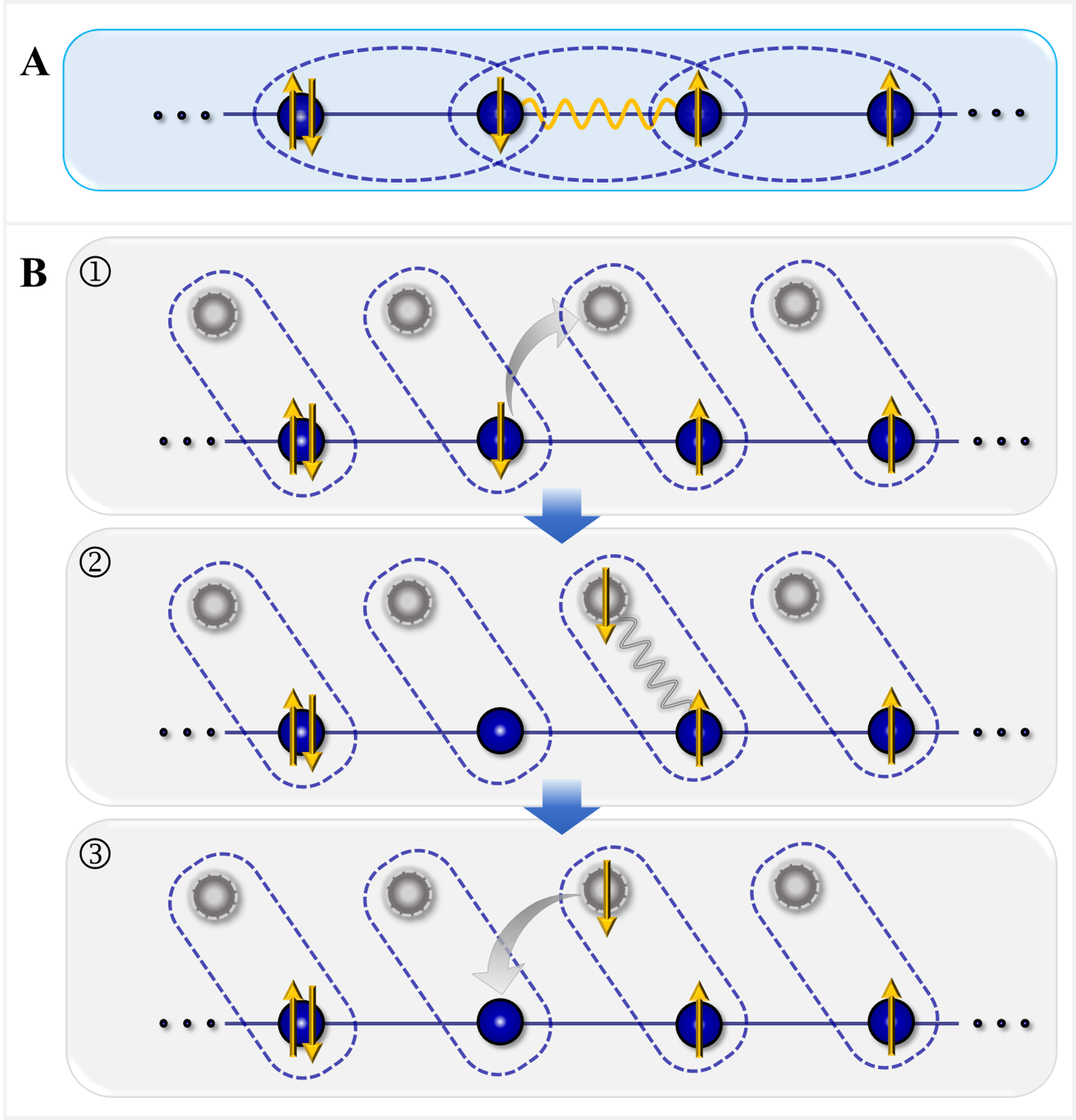
Figure 1: Representation of the density-density interaction in the extended Hubbard model in dimension $D=1$. The blue bullets represent the physical electronic degrees of freedom and the gray bullets represent the ghost particles. Panel A (Eq. (1)): The density-density interaction (yellow wavy line) is non-local. Panel B (Eq. (3)): The density-density interaction is effectively mediated by the virtual processes 1,2,3, involving the ghost degrees of freedom. The interaction (gray wavy line) is local, i.e., it couples only ghost and physical degrees of freedom belonging to the same unit cell.

III Local bottom-up effective theory of the extended Hubbard model

Before discussing realistic multi-orbital systems, let us consider the periodic single-band extended Hubbard model on a $D$-dimensional hypercubic lattice:

$$\hat{H}_{UV}=\hat{H}_{U}+\frac{V}{2}\sum_{\langle ij\rangle}\hat{n}_{i}\hat{n}_{j}\,,$$ (1)

where $\hat{H}_{U}$ is the Hubbard Hamiltonian:

$$\hat{H}_{U}=-t\sum_{\langle ij\rangle\sigma}c^{\dagger}_{i\sigma}c^{\phantom{\dagger}}_{j\sigma}+U\sum_{i}\hat{n}_{i\uparrow}\hat{n}_{i\downarrow}-\mu\sum_{i}\hat{n}_{i}\,;$$ (2)

the symbol $\langle ij\rangle$ indicates the summation over all nearest-neighbour pairs (so that each pair is counted twice); $c^{\dagger}_{i\sigma}$, $c^{\phantom{\dagger}}_{i\sigma}$ are the annihiliation and creation operators of electrons of spin $\sigma\in\{\uparrow,\downarrow\}$ at the atomic site $i$; $\hat{n}_{i\sigma}=c^{\dagger}_{i\sigma}c^{\phantom{\dagger}}_{i\sigma}$ and $\hat{n}_{i}=\hat{n}_{i\uparrow}+\hat{n}_{i\downarrow}$. The non-local operator proportional to $V>0$ is called “density-density interaction”. Campbell et al. (1990)

The key distinctive feature of the non-local interactions, such as the density-density terms in Eq. (1), is that they make it impossible to partition the system into distinct subsystems coupled only by quadratic operators. For example, the partitions enclosed by blue dashed lines in Fig. 1-A are not distinct, as they overlap with each other. In many QE theories, this makes it very challenging to model accurately the coupling between the subsystems and their respective environments. In particular, this is a well-known obstacle within many widely-used QE embedding methods (such as DMFT, RISB and the GA). To solve this cardinal problem, here we design an effective theory satisfying the following conditions:

• Locality, i.e., the existence of a partition into finite subsystems coupled only quadratically.

• Equivalence to Eq (1), i.e., with the property of reproducing exactly its physics for all $U,t,\mu,V$.

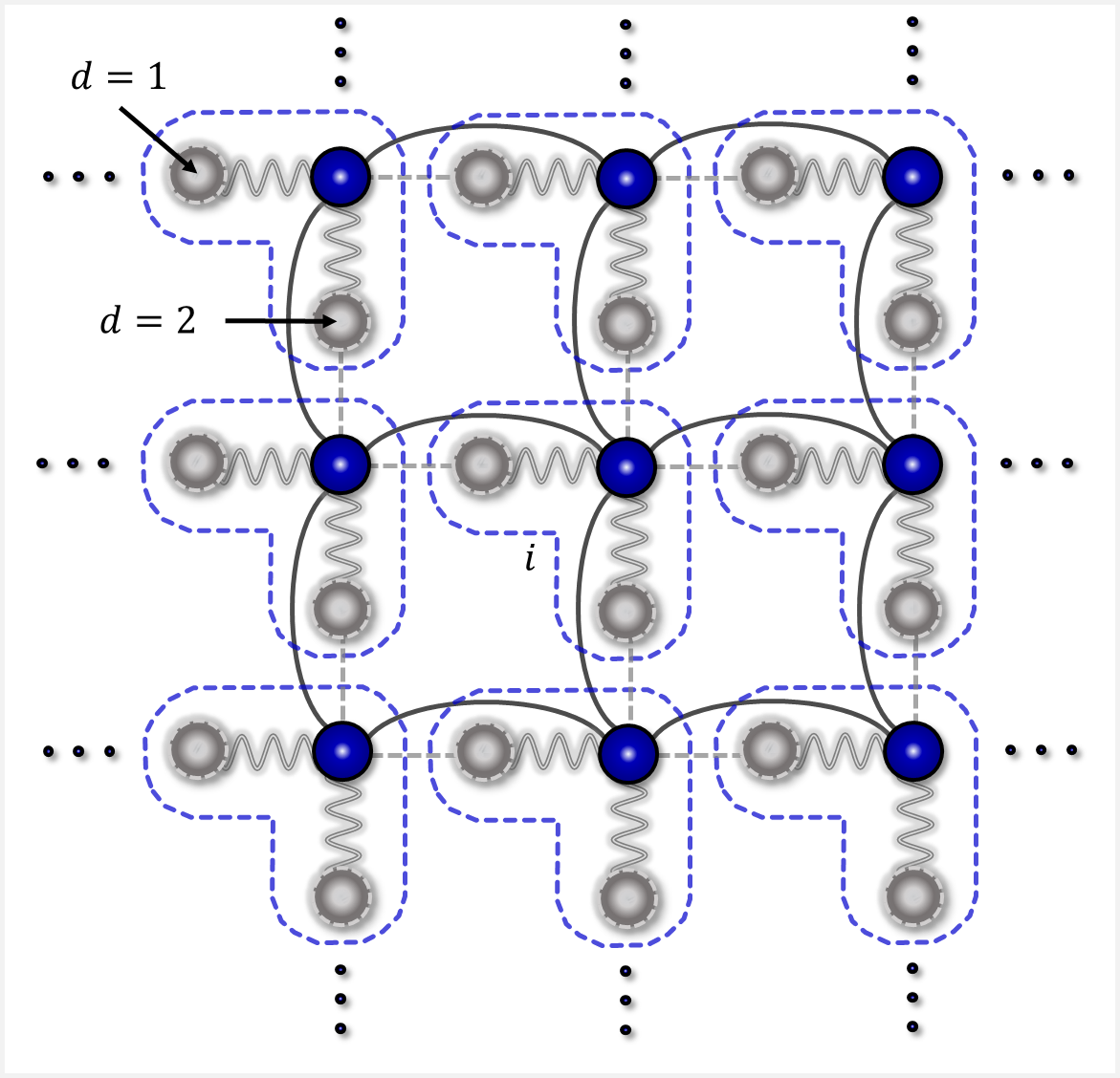
Figure 2: Representation of the effective bottom-up Hamiltonian [Eq. (3)] for a square lattice ($D=2$). The blue bullets represent the physical electronic degrees of freedom and the gray bullets (placed on the corresponding lattice links) represent the ghost particles. The ghost modes placed on the horizontal links have label $d=1$, while the ghost modes placed on the vertical links have label $d=2$ The lattice unit cell, enclosed by dashed lines, have label $i$. The density-density interactions between ghost and fermionic modes are indicated by gray wavy lines, the hopping between physical modes is indicated by continue black lines, the hopping between physical and ghost modes is indicated by gray dashed lines.

As we are going to show, such construction can be realized starting from the following Hamiltonian, represented in Fig. 2 for dimension $D=2$:

$$\hat{H}^{\gamma\tau}_{UV} =\hat{H}_{U}+\tau D\sum_{i}\hat{n}_{i}+\gamma\tau\sum_{i\sigma}\sum_{d=1}^{D}\left(c^{\dagger}_{i\sigma}g^{\phantom{\dagger}}_{i+e_{d}d\sigma}\!+\!\text{H.c}.\right)$$

$$+\gamma^{2}\sum_{i}\!\sum_{d=1}^{D}\left(\tau\,\hat{n}_{id}+V\,\hat{n}_{id}\hat{n}_{i}\right)\,,$$ (3)

where we have introduced $D$ auxiliary fermionic degrees of freedom $g^{\dagger}_{id\sigma}$, $g^{\phantom{\dagger}}_{id\sigma}$ for each unit cell $i$ and spin $\sigma$; $\hat{n}_{id}=\sum_{\sigma}g^{\dagger}_{id\sigma}g^{\phantom{\dagger}}_{id\sigma}$ and $e_{d}$ is the $D$-dimensional vector with all entries equal to $0$ except for the $d$-th component, which is $1$. From now on, we will refer to the auxiliary fermionic particles as the “ghost” degrees of freedom and to Eq. (3) as the “effective bottom-up theory” of Eq. (1).

The fact that Eq. (3) is local (condition 1) stems from the fact that all interaction operators carry the same unit-cell label $i$. This is also shown in Fig. 2, where the subsystems indicated by the blue dashed lines interact only quadratically. Note that the ghost modes (gray dots) are associated with the links connecting the lattice sites (blue dots). This structure is analogue to the quantum link approach to lattice gauge theories, where the fermionic fields are placed on the lattice sites, while the bosonic gauge fields are placed on the links. Wilson (1974) This analogy will be discussed further below.

Let us now focus on the equivalence to Eq. (1) (condition 2). As we are going to show, for $\tau\rightarrow\infty$ and $\gamma\rightarrow\infty$, $\hat{H}^{\gamma\tau}_{UV}$ reproduces exactly the physics of the extended Hubbard model [Eq. (1)]. In particular, this means that, for all physical observables $\hat{O}$ (constructed with $c^{\phantom{\dagger}}_{i\sigma}$, $c^{\dagger}_{i\sigma}$):

$$\lim_{\tau\rightarrow\infty}\lim_{\gamma\rightarrow\infty}\langle\Psi_{\gamma\tau}|\,\hat{O}\,|\Psi_{\gamma\tau}\rangle=\langle\Psi|\,\hat{O}\,|\Psi\rangle\,,$$ (4)

where $|\Psi_{\gamma\tau}\rangle$ is the ground state of Eq. (3) and $|\Psi\rangle$ is the ground state of Eq. (1).

Before demonstrating formally this fact, it is insightful to describe intuitively the key physical concept underlying the construction of Eq. (3): The non-local interactions between the physical electronic modes $c^{\phantom{\dagger}}_{i\sigma}$, $c^{\dagger}_{i\sigma}$ (Fig. 1-A) can be viewed as if they were mediated by the ghost fermions (represented by the operators $g^{\phantom{\dagger}}_{id\sigma}$, $g^{\dagger}_{id\sigma}$). Specifically, in $\hat{H}^{\gamma\tau}_{UV}$ the effect of $V$ is the outcome of the following second-order sequence of processes (Fig. 1-B): (1) a non-local hopping between physical and ghost modes, (2) a local density-density interaction between ghost and physical particles and (3) a second non-local hopping between physical and ghost modes.

Let us now prove this result mathematically. We define $P$ the projector over the “physical” space $\mathcal{V}_{P}$ generated only by $c^{\phantom{\dagger}}_{i\sigma}$, $c^{\dagger}_{i\sigma}$, i.e., where all ghost-particle occupation numbers are $0$. The projector over the auxiliary space generated by the eigenstates of $\hat{n}_{g}=\sum_{id}\hat{n}_{id}$ with eigenvalue $n_{g}\geq 1$ is $Q=1-P$. From the Schrödinger equation for Eq. (3), we deduce that the eigenstates of Eq. (3) satisfy the following equation:

$$\hat{H}_{\text{eff}}^{UV,\gamma\tau}[E_{\gamma\tau}]\,P|\Psi_{\gamma\tau}\rangle=E_{\gamma\tau}\,P|\Psi_{\gamma\tau}\rangle\,,$$ (5)

where $E_{\gamma\tau}$ is a generic eigenvalue of Eq. (3) and:

$$\hat{H}_{\text{eff}}^{UV,\gamma\tau}[E_{\gamma\tau}] =P\hat{H}_{UV}^{\gamma\tau}P+P\hat{H}_{UV}^{\gamma\tau}Q\frac{1}{E_{\gamma\tau}-Q\hat{H}_{UV}^{\gamma\tau}Q}Q\hat{H}_{UV}^{\gamma\tau}P$$

$$=\hat{H}_{U}+\tau D\sum_{i}\hat{n}_{i}+\sum_{id\sigma}c^{\dagger}_{i\sigma}\frac{\tau^{2}}{\gamma^{-2}E_{\gamma\tau}-\gamma^{-2}\big{[}\hat{H}_{U}+\tau D\,\hat{n}_{i+e_{d}}\big{]}+\left(\tau+V\hat{n}_{i}\right)}c^{\phantom{\dagger}}_{i\sigma}\,.$$ (6)

Note that Eq. (5) —with $\hat{H}_{\text{eff}}^{UV,\gamma\tau}[E_{\gamma\tau}]$ given by the first line of Eq. (6)— is an exact identity valid for all Hamiltonians, see Ref. Mila and Schmidt, 2011. The second line of Eq. (6) is obtained by using that, for our specific Hamiltonian, each term of $P\hat{H}_{UV}^{\gamma\tau}Q$ can rise the occupation number of only one of the ghost modes (from $0$ to $1$).

It is important to note that, at any finite $\gamma$, the effective Hamiltonian [Eq. (6)] depends itself on $E_{\gamma\tau}$. To understand how Eq (6) simplifies for $\gamma\rightarrow\infty$ (at fixed $\tau>0$), we need to estimate how the eigenvalues $E_{\gamma\tau}$ of Eq. (3) behave in this limit. As we are going to show, the spectra of Eq. (3) is divided in 2 sectors: a the low-energy (physical) sector, such that:

$$\lim_{\gamma\rightarrow\infty}\gamma^{-2}E_{\gamma\tau}=0\,,$$ (7)

and a high-energy (auxiliary) sector, with eigenvalues diverging as $\tau\gamma^{2}$. To prove this fact, starting from Eq. (3), we note that $\gamma^{-2}\hat{H}^{\gamma\tau}_{UV}$ can be expressed as follows:

$$\gamma^{-2}\hat{H}^{\gamma\tau}_{UV}=\hat{h}^{\tau}_{UV}+\hat{r}^{\tau}_{UV}(\gamma)\,,$$ (8)

where:

$$\hat{h}^{\tau}_{UV} =\sum_{i}\!\sum_{d=1}^{D}\left(\tau\,\hat{n}_{id}+V\,\hat{n}_{id}\hat{n}_{i}\right)\,,$$ (9)

$$\hat{r}^{\tau}_{UV}(\gamma) =\gamma^{-1}\tau\sum_{i\sigma}\sum_{d=1}^{D}\left(c^{\dagger}_{i\sigma}g^{\phantom{\dagger}}_{i+e_{d}d\sigma}+\text{H.c}.\right)$$

$$+\gamma^{-2}\left(\hat{H}_{U}+\tau D\sum_{i}\hat{n}_{i}\right)\,.$$ (10)

We note that $\hat{h}^{\tau}_{UV}$ assigns an energy cost $\propto\tau>0$ to all unphysical configurations (with non-zero occupied ghost modes), while its ground space coincides with the physical subspace $\mathcal{V}_{P}$ (where, by definition, all ghost modes are empty). Since $\hat{r}^{\tau}_{UV}(\gamma)$ vanishes for $\gamma\rightarrow\infty$, the low-energy eigenvalues $\gamma^{-2}E_{\gamma\tau}$ of Eq. (8) satisfy Eq. (7). Instead, $E_{\gamma\tau}$ diverges as $\tau\gamma^{2}$ for the unphysical states. For the same reason, the low-energy eigenstates $|\Psi_{\gamma\tau}\rangle$ become equal to $P|\Psi_{\gamma\tau}\rangle$ in this limit.

By substituting Eq. (7) in Eq. (6), we deduce that, in the low-energy sector, Eq. (5) reduces to an ordinary (energy-independent) Schrödinger equation for $\gamma\rightarrow\infty$, with respect to the following effective Hamiltonian:

$$\hat{H}_{\text{eff}}^{UV,\tau}=\hat{H}_{U}+\tau D\sum_{i}\hat{n}_{i}-\sum_{id\sigma}c^{\dagger}_{i\sigma}\frac{\tau^{2}}{\tau+V\hat{n}_{i+e_{d}}}c^{\phantom{\dagger}}_{i\sigma}\,.$$ (11)

Let us now evaluate the limit of Eq. (11) for $\tau\rightarrow\infty$. We note that, if $\tau$ is sufficiently large, the following equation holds:

$$\frac{\tau^{2}}{\tau+V\hat{n}_{i+e_{d}}}=\tau\left[1-\frac{V}{\tau}\hat{n}_{i+e_{d}}+\sum_{l=2}^{\infty}\left(-\frac{V}{\tau}\hat{n}_{i+e_{d}}\right)^{l}\right]\,.$$ (12)

In fact, since the maximum eigenvalue of $\hat{n}_{i+e_{d}}$ is $2$, the geometric series is guaranteed to converge for $\forall\,\tau>2V$. By substituting Eq. (12) in Eq. (11), we obtain:

$$\hat{H}_{\text{eff}}^{UV,\tau}=\hat{H}_{UV}+\hat{o}_{V}(\tau)\,,$$ (13)

which coincides with Eq. (1) up to a perturbation of order $\hat{o}_{V}(\tau)\sim V^{2}\tau^{-1}$, thatt vanishes for $\tau\rightarrow\infty$.

In summary, for $\gamma\rightarrow\infty$ the states with non-zero ghost occupations are gapped out (as their energy diverges as $\tau\gamma^{2}$). On the other hand, they mediate the desired non-local density-density interaction of Eq. (1) within the physical space, by means of second-order (virtual) processes. At finite $\tau$, these virtual processes generate also undesired additional interactions (because of the subleading terms of order $\geq 2$ in the geometric series [Eq. (12)]). But all spurious terms vanish as $2V/\tau^{2}$ for $\tau\rightarrow\infty$, while the desired density-density interaction remains. In other words, the spurious terms associated with deviations from the extended Hubbard model are suppressed by a factor $\propto(V/\tau)^{2}$ with respect to the density-density interaction. Therefore, in these limits, the low-energy sector of Eq. (3) reproduces exactly the physics of Eq. (1), $\forall\,U,t,\mu,V$.

We point out that, in the last step in Eq (6), we used the fact that the ghost degrees of freedom in Eq. (1) are placed on the links (analogously to lattice gauge theories. Wilson (1974)) In fact, linking a ghost fermion to multiple physical modes would generate additional second-order processes —and, in turn, additional long-range interactions not present in the original extended Hubbard Hamiltonian [Eq. (1)]. This explains why the non-local interactions along different directions in $\hat{H}_{UV}^{\gamma\tau}$ have to be mediated by distinct ghost particles, identified by the label $d$. Note also that, since the ghost fermions are placed on the links, Eq. (3) preserves the translational invariance of the system $\forall\,\gamma,\tau$ —as opposed to classic cluster approaches, Kotliar et al. (2001); Maier et al. (2005); Senechal et al. (2000); Potthoff et al. (2003); Lichtenstein and Katsnelson (2000) where the problem of breaking artificially the translational symmetry cannot be avoided.

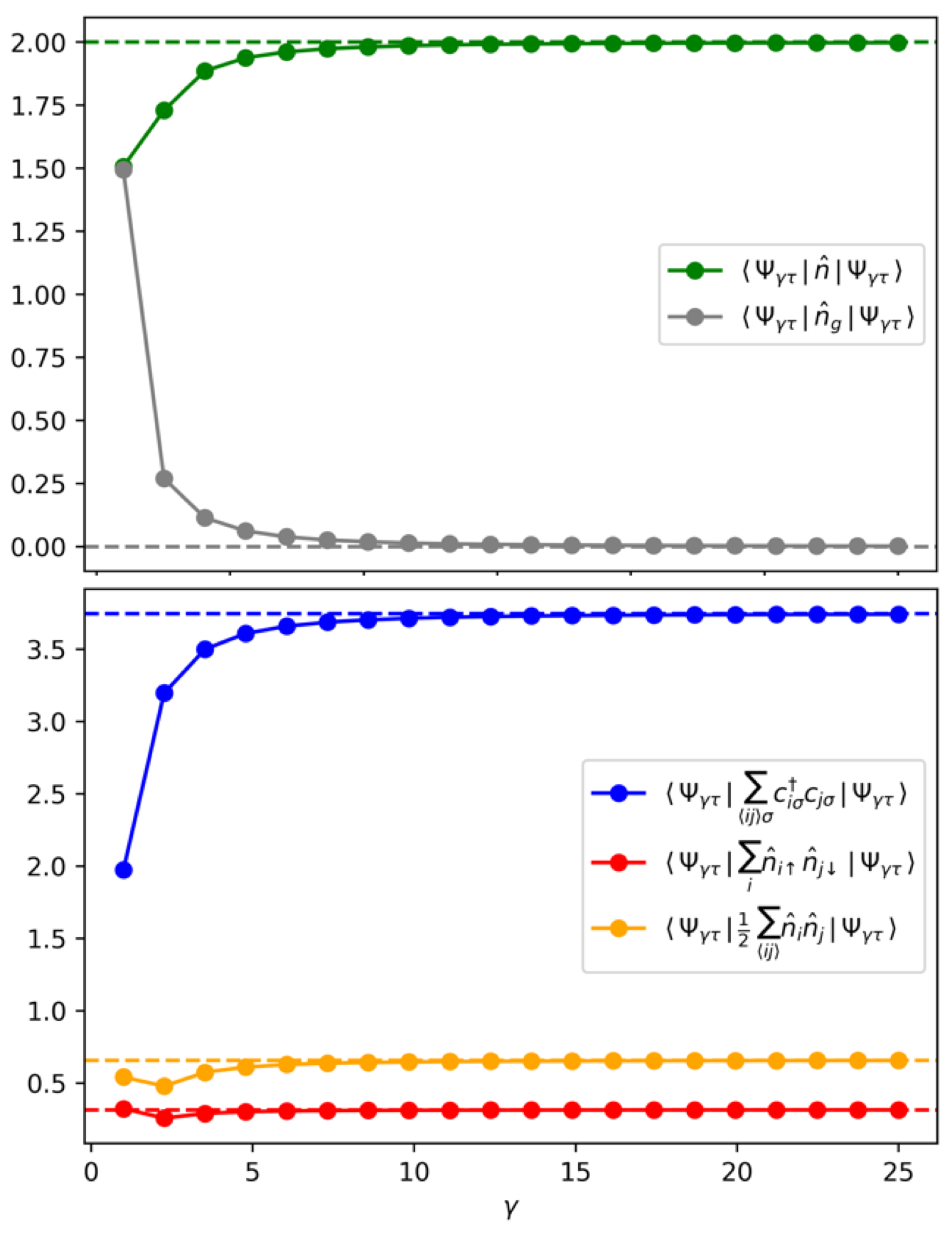
Figure 3: Solution of the 4-sites single-band extended Hubbard model at half filling for $U=3$ and $V=1.5$, where $t$ is set as the energy unit. The dotted lines indicate quantities calculated directly from Eq. (1), while the bullet points are quantities calculated using the effective bottom-up Hamiltonian [Eq. (3)], for different values of $\gamma$ and ${2V}{\tau^{-1}}=10^{-2}$. Top panel: Physical occupation (green) and ghost occupation (gray). Bottom panel: Hopping operator (blue), double occupancy (red) and density-density operator (orange).

To illustrate the implications of our result in a minimal setting, in Fig. 3 we present numerical calculations of a half-filled 1-dimensional extended Hubbard model $\hat{H}_{UV}$ consisting of 4 physical sites. Note that, for this relatively small system, both the original Hamiltonian and the corresponding effective Hamiltonian $\hat{H}^{\gamma\tau}_{UV}$ can be diagonalized exactly. As an example, we set $t$ as unit of energy, $U=3$ and $V=1.5$. In all calculations we set the parameter of the geometric expansion in Eq. (12) to ${2V}{\tau^{-1}}=10^{-2}$. In the top panel is shown the behavior, as a function of $\gamma$, of the physical occupancy $\langle\Psi_{\gamma\tau}|\,\hat{n}\,|\Psi_{\gamma\tau}\rangle$ (green line) and of the occupation of the ghost modes $\langle\Psi_{\gamma\tau}|\,\hat{n}_{d}\,|\Psi_{\gamma\tau}\rangle$ (gray line). In the bottom panel are shown the corresponding expectation values for a few physical observables. Consistently with Eq. (4), the numerical calculations confirm that the “spurious” charge transfer between physical and ghost degrees of freedom vanishes for large $\gamma$, where the ghost modes are gapped-out and, therefore, the corresponding occupancy vanishes. Furthermore, all expectation values converge to the correct limit for $\gamma\rightarrow\infty$, as expected. The exact-diagonalization calculations were performed using the open-source software “OpenFermion”. McClean et al. (2020)

Generalization to multi-orbital systems

The procedure utilized above within the context of the single-band extended Hubbard model can be straightforwardly generalized to realistic multi-orbital Hamiltonians. For example, let us consider the following $D$-dimensional system:

$$\hat{H}_{UV}=\hat{H}_{U}+\frac{1}{2}\sum_{<ij>}\sum_{\alpha\beta\gamma\delta=1}^{\nu}{V}_{\alpha\beta\gamma\delta}\,c^{\dagger}_{i\alpha}c^{\phantom{\dagger}}_{i\beta}c^{\dagger}_{j\gamma}c^{\phantom{\dagger}}_{j\delta}\,,$$ (14)

where $\hat{H}_{U}$ is any multi-orbital Hamiltonian with purely-local interactions, the labels $\alpha,\beta,\gamma,\delta$ represent both orbital and spin degrees of freedom and the coefficients $V_{\alpha\beta\gamma\delta}$ parametrize a generic density-density operator —which is typically the largest contribution to non-local interactions in real solids and molecules. Campbell et al. (1990) It can be readily shown that the effective bottom-up theory of Eq. (14) is the following:

$$\hat{H}_{UV}^{\gamma\tau} =\hat{H}_{U}+\tau D\sum_{i}\hat{n}_{i}+\gamma\tau\sum_{id\alpha}\left(c^{\dagger}_{i\alpha}g^{\phantom{\dagger}}_{i+e_{d}d\alpha}+\text{H.c.}\right)$$

$$+\gamma^{2}\sum_{id}\left[\tau\,\hat{n}_{id}+\sum_{\alpha\beta\gamma\delta}V_{\alpha\beta\gamma\delta}\,g^{\dagger}_{id\alpha}g^{\phantom{\dagger}}_{id\beta}c^{\dagger}_{i\gamma}c^{\phantom{\dagger}}_{i\delta}\right]\,,$$ (15)

where:

$$\hat{n}_{i} =\sum_{\alpha}c^{\dagger}_{i\alpha}c^{\phantom{\dagger}}_{i\alpha}$$ (16)

$$\hat{n}_{id} =\sum_{\alpha}g^{\dagger}_{id\alpha}g^{\phantom{\dagger}}_{id\alpha}\,.$$ (17)

Note that, as for the single-orbital case, $\hat{H}_{UV}^{\gamma\tau}$ becomes equivalent to $\hat{H}_{UV}$ for ${\gamma\rightarrow\infty}$ and ${\tau\rightarrow\infty}$ (where, as before, the limit for ${\gamma\rightarrow\infty}$ is taken first).

We point out that the theoretical construction derived in this work is not restricted to hypercubic periodic lattices, but can be extended to systems with arbitrary structures (also without translational symmetry). Furthermore, also the Coulomb interactions beyond first nearest neighbours can be described, in a similar fashion, by introducing longer-range hopping operators between physical and ghost degrees of freedom. Our approach may be applicable also for studying real crystals and molecules, e.g., using the interfaces already available for performing this type of calculations. Haule et al. (2010); Pham et al. (2020); Deng et al. (2009) In fact, treating systematically beyond the mean-field level also the dominant (e.g., first-nearest-neighbor) contributions of the non-local interactions may improve substantially the accuracy of these methods. In this respect, applications in combination with HF+QE frameworks Pham et al. (2020) (which do not require to introduce any adjustable parameters) are particularly appealing.

IV Conclusions

In summary, we have shown that all multi-orbital systems represented by Eq. (14) —which includes all local and the largest non-local contributions of most real solids and molecules Campbell et al. (1990)— can be equivalently described by solving higher-dimensional fermionic systems with purely local interactions, see Eq. (15). This exact result is analogue to the quantum link approach to lattice gauge theories, where the fermionic fields are placed on the lattice sites, while the bosonic gauge fields are placed on the links. Wilson (1974) The dual relationship between non-local and local interactions, demonstrated here, provides us with a rigorous alternative direction of interpretation. Furthermore, the possibility of using auxiliary fermions for decoupling the non-local interactions may allow us to develop new methods for including these effects in practical calculations —complementary to the available computational frameworks. In fact, many of the existing state-of-the-art QE approaches are based on the so-called Hubbard-Stratonovich transformation, Rohringer et al. (2018) which utilizes auxiliary bosons, instead of fermions. Computationally, the main cost of performing calculations of our dual model would be that introducing additional fermionic degrees of freedom increases the dimension of the EH. However, within QE methods such as DMET and the GA (where the bath of the EH is as large as the impurity Lanatà et al. (2015); Knizia and Chan (2012)), applications to models with up to 3 correlated orbitals per atom may be already feasible using exact diagonalization or state-of-the-art quantum chemistry methods Zhang and Grüneis (2019); Bartlett and Musiał (2007); Parrish et al. (2017) as impurity solvers. Furthermore, thanks to the rapidly-evolving technological developments based on machine learning Arsenault et al. (2014); Rogers et al. (2020) and quantum-computing, O’Malley et al. (2016); Kandala et al. (2017); Peruzzo et al. (2014); Wecker et al. (2015); Babbush et al. (2018); Hempel et al. (2018); Grimsley et al. (2019); Yao et al. (2020) it may soon become possible to apply this framework also to arbitrary d-electron and f-electron systems.

V Acknowledgements

We thank Gabriel Kotliar, Garry Goldstein, Ove Christiansen, Vladimir Dobrosavljević, and Yongxin Yao for useful discussions. We gratefully acknowledge funding from VILLUM FONDEN through the Villum Experiment project 00028019 and the Centre of Excellence for Dirac Materials (Grant. No. 11744). We also thank support from the Novo Nordisk Foundation through the Exploratory Interdisciplinary Synergy Programme project NNF19OC0057790.

References

- Kent and Kotliar (2018) Paul R. C. Kent and Gabriel Kotliar, “Toward a predictive theory of correlated materials,” Science 361, 348–354 (2018).
- Furukawa et al. (2015) Tetsuya Furukawa, Kazuya Miyagawa, Hiromi Taniguchi, Reizo Kato, and Kazushi Kanoda, “Quantum criticality of mott transition in organic materials,” Nature Physics 11, 221–224 (2015).
- McKenzie (1997) Ross H. McKenzie, “Similarities between organic and cuprate superconductors,” Science 278, 820–821 (1997).
- Imada et al. (1998) Masatoshi Imada, Atsushi Fujimori, and Yoshinori Tokura, “Metal-insulator transitions,” Rev. Mod. Phys. 70, 1039–1263 (1998).
- Lee et al. (2006) Patrick A. Lee, Naoto Nagaosa, and Xiao-Gang Wen, “Doping a mott insulator: Physics of high-temperature superconductivity,” Rev. Mod. Phys. 78, 17–85 (2006).
- Paglione and Greene (2010) Johnpierre Paglione and Richard L. Greene, “High-temperature superconductivity in iron-based materials,” Nature Physics 6, 645–658 (2010).
- Sun and Chan (2016) Qiming Sun and Garnet Kin-Lic Chan, “Quantum embedding theories,” Accounts of Chemical Research 49, 2705–2712 (2016).
- Kotliar et al. (2006) G. Kotliar, S. Y. Savrasov, K. Haule, V. S. Oudovenko, O. Parcollet, and C. A. Marianetti, “Electronic structure calculations with dynamical mean-field theory,” Rev. Mod. Phys. 78, 865 (2006).
- Held et al. (2006) K. Held, A. Nekrasov, G. Keller, V. Eyert, N. Blümer, A. K. McMahan, R. T. Scalettar, Th. Pruschke, V. I. Anisimov, and D. Vollhardt, “Realistic investigations of correlated electron systems with LDA+DMFT,” Phys. Stat. Sol. (B) 243, 2599 (2006).
- Georges et al. (1996) A. Georges, G. Kotliar, W. Krauth, and M. J. Rozenberg, “Dynamical mean-field theory of strongly correlated fermion systems and the limit of infinite dimensions,” Rev. Mod. Phys. 68, 13 (1996).
- Anisimov and Izyumov (2010) V. Anisimov and Y. Izyumov, Electronic Structure of Strongly Correlated Materials (Springer, 2010).
- Gutzwiller (1965) M. C. Gutzwiller, “Correlation of Electrons in a Narrow Band,” Phys. Rev. 137, A1726 (1965).
- Bünemann et al. (1998) J. Bünemann, W. Weber, and F. Gebhard, “Multiband Gutzwiller wave functions for general on-site interactions,” Phys. Rev. B 57, 6896 (1998).
- Fabrizio (2007) M. Fabrizio, “Gutzwiller description of non-magnetic Mott insulators: Dimer lattice model,” Phys. Rev. B 76, 165110 (2007).
- Deng et al. (2009) X.-Y. Deng, L. Wang, X. Dai, and Z. Fang, “Local density approximation combined with Gutzwiller method for correlated electron systems: Formalism and applications,” Phys. Rev. B 79, 075114 (2009).
- Lanatà et al. (2008) N. Lanatà, P. Barone, and M. Fabrizio, “Fermi-surface evolution across the magnetic phase transition in the Kondo lattice model,” Phys. Rev. B 78, 155127 (2008).
- Lanatà et al. (2012) N. Lanatà, H. U. R. Strand, X. Dai, and B. Hellsing, “Efficient implementation of the Gutzwiller variational method,” Phys. Rev. B 85, 035133 (2012).
- Ho et al. (2008) K. M. Ho, J. Schmalian, and C. Z. Wang, “Gutzwiller density functional theory for correlated electron systems,” Phys. Rev. B 77, 073101 (2008).
- Lanatà et al. (2015) Nicola Lanatà, Yong Xin Yao, Cai-Zhuang Wang, Kai-Ming Ho, and Gabriel Kotliar, “Phase diagram and electronic structure of praseodymium and plutonium,” Phys. Rev. X 5, 011008 (2015).
- Lanatà et al. (2017a) Nicola Lanatà, Tsung-Han Lee, Yong-Xin Yao, and Vladimir Dobrosavljević, “Emergent bloch excitations in mott matter,” Phys. Rev. B 96, 195126 (2017a).
- Knizia and Chan (2012) G. Knizia and G. K.-L. Chan, “Density matrix embedding: A simple alternative to dynamical mean-field theory,” Phys. Rev. Lett. 109, 186404 (2012).
- Kotliar and Ruckenstein (1986) G. Kotliar and A. E. Ruckenstein, “New functional integral approach to strongly correlated Fermi systems: The Gutzwiller Approximation as a Saddle Point,” Phys. Rev. Lett. 57, 1362 (1986).
- Lechermann et al. (2007) F. Lechermann, A. Georges, G. Kotliar, and O. Parcollet, “Rotationally invariant slave-boson formalism and momentum dependence of the quasiparticle weight,” Phys. Rev. B 76, 155102 (2007).
- Li et al. (1989) T. Li, P. Wölfle, and P. J. Hirschfeld, “Spin-rotation-invariant slave-boson approach to the Hubbard model,” Phys. Rev. B 40, 6817 (1989).
- Lanatà et al. (2017b) Nicola Lanatà, Yongxin Yao, Xiaoyu Deng, Vladimir Dobrosavljević, and Gabriel Kotliar, “Slave boson theory of orbital differentiation with crystal field effects: Application to ,” Phys. Rev. Lett. 118, 126401 (2017b).
- Bockstedte et al. (2018) Michel Bockstedte, Felix Schütz, Thomas Garratt, Viktor Ivády, and Adam Gali, “Ab initio description of highly correlated states in defects for realizing quantum bits,” npj Quantum Materials 3, 31 (2018).
- Dvorak et al. (2019) Marc Dvorak, Dorothea Golze, and Patrick Rinke, “Quantum embedding theory in the screened coulomb interaction: Combining configuration interaction with ,” Phys. Rev. Materials 3, 070801 (2019).
- Hansmann et al. (2013) P. Hansmann, T. Ayral, L. Vaugier, P. Werner, and S. Biermann, “Long-range coulomb interactions in surface systems: A first-principles description within self-consistently combined and dynamical mean-field theory,” Phys. Rev. Lett. 110, 166401 (2013).
- Wehling et al. (2011) T. O. Wehling, E. Şaşıoğlu, C. Friedrich, A. I. Lichtenstein, M. I. Katsnelson, and S. Blügel, “Strength of effective coulomb interactions in graphene and graphite,” Phys. Rev. Lett. 106, 236805 (2011).
- Schüler et al. (2013) M. Schüler, M. Rösner, T. O. Wehling, A. I. Lichtenstein, and M. I. Katsnelson, “Optimal hubbard models for materials with nonlocal coulomb interactions: Graphene, silicene, and benzene,” Phys. Rev. Lett. 111, 036601 (2013).
- Onari et al. (2004) Seiichiro Onari, Ryotaro Arita, Kazuhiko Kuroki, and Hideo Aoki, “Phase diagram of the two-dimensional extended hubbard model: Phase transitions between different pairing symmetries when charge and spin fluctuations coexist,” Phys. Rev. B 70, 094523 (2004).
- Poteryaev et al. (2004) A. I. Poteryaev, A. I. Lichtenstein, and G. Kotliar, “Nonlocal coulomb interactions and metal-insulator transition in : A cluster approach,” Phys. Rev. Lett. 93, 086401 (2004).
- van Loon et al. (2018) Erik G. C. P. van Loon, Malte Rösner, Gunnar Schönhoff, Mikhail I. Katsnelson, and Tim O. Wehling, “Competing coulomb and electron-phonon interactions in nbs2,” npj Quantum Materials 3, 32 (2018).
- Grimme et al. (2016) Stefan Grimme, Andreas Hansen, Jan Gerit Brandenburg, and Christoph Bannwarth, “Dispersion-corrected mean-field electronic structure methods,” Chemical Reviews 116, 5105–5154 (2016).
- Cerný et al. (2008) Jirí Cerný, Martin Kabelác, and Pavel Hobza, “Double-helical - ladder structural transition in the b-dna is induced by a loss of dispersion energy,” Journal of the American Chemical Society 130, 16055–16059 (2008).
- Ayral et al. (2013) Thomas Ayral, Silke Biermann, and Philipp Werner, “Screening and nonlocal correlations in the extended hubbard model from self-consistent combined GW and dynamical mean field theory,” Phys. Rev. B 87, 125149 (2013).
- Terletska et al. (2017) Hanna Terletska, Tianran Chen, and Emanuel Gull, “Charge ordering and correlation effects in the extended hubbard model,” Phys. Rev. B 95, 115149 (2017).
- Rohringer et al. (2018) G. Rohringer, H. Hafermann, A. Toschi, A. A. Katanin, A. E. Antipov, M. I. Katsnelson, A. I. Lichtenstein, A. N. Rubtsov, and K. Held, “Diagrammatic routes to nonlocal correlations beyond dynamical mean field theory,” Rev. Mod. Phys. 90, 025003 (2018).
- Vučičević et al. (2017) J. Vučičević, T. Ayral, and O. Parcollet, “TRILEX and GW+EDMFT approach to -wave superconductivity in the Hubbard model,” Phys. Rev. B 96, 104504 (2017).
- Rubtsov et al. (2008) A. N. Rubtsov, M. I. Katsnelson, and A. I. Lichtenstein, “Dual fermion approach to nonlocal correlations in the hubbard model,” Phys. Rev. B 77, 033101 (2008).
- Biermann et al. (2003) S. Biermann, F. Aryasetiawan, and A. Georges, “First-principles approach to the electronic structure of strongly correlated systems: Combining the GW approximation and Dynamical Mean-Field Theory,” Phys. Rev. Lett. 90, 086402 (2003).
- Zhang et al. (1988) F C Zhang, C Gros, T M Rice, and H Shiba, “A renormalised hamiltonian approach to a resonant valence bond wavefunction,” Superconductor Science and Technology 1, 36–46 (1988).
- Ogata and Himeda (2003) Masao Ogata and Akihiro Himeda, “Superconductivity and antiferromagnetism in an extended gutzwiller approximation for t-j model: Effect of double-occupancy exclusion,” Journal of the Physical Society of Japan 72, 374–391 (2003).
- Yao et al. (2014) Y. X. Yao, J. Liu, C. Z. Wang, and K. M. Ho, “Correlation matrix renormalization approximation for total-energy calculations of correlated electron systems,” Phys. Rev. B 89, 045131 (2014).
- Zhao et al. (2018) Xin Zhao, Jun Liu, Yong-Xin Yao, Cai-Zhuang Wang, and Kai-Ming Ho, “Correlation matrix renormalization theory for correlated-electron materials with application to the crystalline phases of atomic hydrogen,” Phys. Rev. B 97, 075142 (2018).
- Fidrysiak et al. (2019) M. Fidrysiak, D. Goc-Jaglo, E. Kadzielawa-Major, P. Kubiczek, and J. Spalek, “Coexistent spin-triplet superconducting and ferromagnetic phases induced by hund’s rule coupling and electronic correlations: Effect of the applied magnetic field,” Phys. Rev. B 99, 205106 (2019).
- Zegrodnik and Spałek (2018) Michał Zegrodnik and Józef Spałek, “Incorporation of charge- and pair-density-wave states into the one-band model of -wave superconductivity,” Phys. Rev. B 98, 155144 (2018).
- Goldstein et al. (2020) Garry Goldstein, Nicola Lanatà, and Gabriel Kotliar, “Extending the gutzwiller approximation to intersite interactions,” Phys. Rev. B 102, 045152 (2020).
- Zhang and Grüneis (2019) Igor Ying Zhang and Andreas Grüneis, “Coupled cluster theory in materials science,” Frontiers in Materials 6, 123 (2019).
- Bartlett and Musiał (2007) Rodney J. Bartlett and Monika Musiał, “Coupled-cluster theory in quantum chemistry,” Rev. Mod. Phys. 79, 291–352 (2007).
- Parrish et al. (2017) Robert M. Parrish, Lori A. Burns, Daniel G. A. Smith, Andrew C. Simmonett, A. Eugene DePrince, Edward G. Hohenstein, Ugur Bozkaya, Alexander Yu Sokolov, Roberto Di Remigio, Ryan M. Richard, Jérôme F. Gonthier, Andrew M. James, Harley R. McAlexander, Ashutosh Kumar, Masaaki Saitow, Xiao Wang, Benjamin P. Pritchard, Prakash Verma, Henry F. Schaefer, Konrad Patkowski, Rollin A. King, Edward F. Valeev, Francesco A. Evangelista, Justin M. Turney, T. Daniel Crawford, and C. David Sherrill, “Psi4 1.1: An open-source electronic structure program emphasizing automation, advanced libraries, and interoperability,” Journal of Chemical Theory and Computation 13, 3185–3197 (2017).
- Arsenault et al. (2014) Louis-Fran çois Arsenault, Alejandro Lopez-Bezanilla, O. Anatole von Lilienfeld, and Andrew J. Millis, “Machine learning for many-body physics: The case of the anderson impurity model,” Phys. Rev. B 90, 155136 (2014).
- Rogers et al. (2020) John Rogers, T.-H. Lee, S. Pakdel, Wenhu Xu, Vladimir Dobrosavljević, Yongxin Yao, Ove Christiansen, and Nicola Lanatà, “Bypassing the computational bottleneck off quantum-embedding theories for strong electron correlations with machine learning,” (2020), arXiv:cond-mat/2006.15227 .
- O’Malley et al. (2016) P. J. J. O’Malley, R. Babbush, I. D. Kivlichan, J. Romero, J. R. McClean, R. Barends, J. Kelly, P. Roushan, A. Tranter, N. Ding, B. Campbell, Y. Chen, Z. Chen, B. Chiaro, A. Dunsworth, A. G. Fowler, E. Jeffrey, E. Lucero, A. Megrant, J. Y. Mutus, M. Neeley, C. Neill, C. Quintana, D. Sank, A. Vainsencher, J. Wenner, T. C. White, P. V. Coveney, P. J. Love, H. Neven, A. Aspuru-Guzik, and J. M. Martinis, “Scalable quantum simulation of molecular energies,” Phys. Rev. X 6, 031007 (2016).
- Kandala et al. (2017) Abhinav Kandala, Antonio Mezzacapo, Kristan Temme, Maika Takita, Markus Brink, Jerry M. Chow, and Jay M. Gambetta, “Hardware-efficient variational quantum eigensolver for small molecules and quantum magnets,” Nature 549, 242–246 (2017).
- Peruzzo et al. (2014) Alberto Peruzzo, Jarrod McClean, Peter Shadbolt, Man-Hong Yung, Xiao-Qi Zhou, Peter J. Love, Alán Aspuru-Guzik, and Jeremy L. O’Brien, “A variational eigenvalue solver on a photonic quantum processor,” Nature Communications 5, 4213 (2014).
- Wecker et al. (2015) Dave Wecker, Matthew B. Hastings, and Matthias Troyer, “Progress towards practical quantum variational algorithms,” Phys. Rev. A 92, 042303 (2015).
- Babbush et al. (2018) Ryan Babbush, Nathan Wiebe, Jarrod McClean, James McClain, Hartmut Neven, and Garnet Kin-Lic Chan, “Low-depth quantum simulation of materials,” Phys. Rev. X 8, 011044 (2018).
- Hempel et al. (2018) Cornelius Hempel, Christine Maier, Jonathan Romero, Jarrod McClean, Thomas Monz, Heng Shen, Petar Jurcevic, Ben P. Lanyon, Peter Love, Ryan Babbush, Alán Aspuru-Guzik, Rainer Blatt, and Christian F. Roos, “Quantum chemistry calculations on a trapped-ion quantum simulator,” Phys. Rev. X 8, 031022 (2018).
- Grimsley et al. (2019) Harper R. Grimsley, Sophia E. Economou, Edwin Barnes, and Nicholas J. Mayhall, “An adaptive variational algorithm for exact molecular simulations on a quantum computer,” Nature Communications 10, 3007 (2019).
- Yao et al. (2020) Yongxin Yao, Feng Zhang, Cai-Zhuang Wang, Kai-Ming Ho, and P. Orth Peter, “Gutzwiller hybrid quantum-classical computing approach for correlated materials,” (2020), arXiv:cond-mat/2003.04211 .
- Foldy and Wouthuysen (1950) Leslie L. Foldy and Siegfried A. Wouthuysen, “On the dirac theory of spin 1/2 particles and its non-relativistic limit,” Phys. Rev. 78, 29–36 (1950).
- Wilson (1975) Kenneth G. Wilson, “The renormalization group: Critical phenomena and the kondo problem,” Rev. Mod. Phys. 47, 773–840 (1975).
- Chernyshev et al. (2004) A. L. Chernyshev, D. Galanakis, P. Phillips, A. V. Rozhkov, and A.-M. S. Tremblay, “Higher order corrections to effective low-energy theories for strongly correlated electron systems,” Phys. Rev. B 70, 235111 (2004).
- Schrieffer and Wolff (1966) J. R. Schrieffer and P. A. Wolff, “Relation between the anderson and kondo hamiltonians,” Phys. Rev. 149, 491–492 (1966).
- Campbell et al. (1990) D. K. Campbell, J. Tinka Gammel, and E. Y. Loh, “Modeling electron-electron interactions in reduced-dimensional materials: Bond-charge coulomb repulsion and dimerization in peierls-hubbard models,” Phys. Rev. B 42, 475–492 (1990).
- Wilson (1974) Kenneth G. Wilson, “Confinement of quarks,” Phys. Rev. D 10, 2445–2459 (1974).
- Mila and Schmidt (2011) F. Mila and K.P. Schmidt, Strong-Coupling Expansion and Effective Hamiltonians. In: Introduction to Frustrated Magnetism. Springer Series in Solid-State Sciences (Springer Series in Solid-State Sciences, vol 164. Springer, Berlin, Heidelberg, 2011).
- Kotliar et al. (2001) G. Kotliar, S. Y. Savrasov, G. Pálsson, and G. Biroli, “Cellular dynamical mean field approach to strongly correlated systems,” Phys. Rev. Lett. 87, 186401 (2001).
- Maier et al. (2005) T. Maier, M. Jarrell, T. Pruschke, and M. H. Hettler, “Quantum cluster theories,” Rev. Mod. Phys. 77, 1027 (2005).
- Senechal et al. (2000) D. Senechal, D. Perez, and M. Pioro-Ladriere, “The spectral weight of the Hubbard model through cluster perturbation theory,” Phys. Rev. Lett. 84, 522 (2000).
- Potthoff et al. (2003) M. Potthoff, M. Aichhorn, and C. Dahnken, “Variational cluster approach to correlated electron systems in low dimensions,” Phys. Rev. Lett. 91, 206402 (2003).
- Lichtenstein and Katsnelson (2000) A. I. Lichtenstein and M. I. Katsnelson, “Antiferromagnetism and d-wave superconductivity in cuprates: A cluster dynamical mean-field theory,” Phys. Rev. B 62, R9283 (2000).
- McClean et al. (2020) Jarrod R McClean, Nicholas C Rubin, Kevin J Sung, Ian D Kivlichan, Xavier Bonet-Monroig, Yudong Cao, Chengyu Dai, E Schuyler Fried, Craig Gidney, Brendan Gimby, Pranav Gokhale, Thomas Häner, Tarini Hardikar, Vojtěch Havlíček, Oscar Higgott, Cupjin Huang, Josh Izaac, Zhang Jiang, Xinle Liu, Sam McArdle, Matthew Neeley, Thomas O’Brien, Bryan O’Gorman, Isil Ozfidan, Maxwell D Radin, Jhonathan Romero, Nicolas P D Sawaya, Bruno Senjean, Kanav Setia, Sukin Sim, Damian S Steiger, Mark Steudtner, Qiming Sun, Wei Sun, Daochen Wang, Fang Zhang, and Ryan Babbush, “OpenFermion: the electronic structure package for quantum computers,” Quantum Science and Technology 5, 034014 (2020).
- Haule et al. (2010) K. Haule, C.-H. Yee, and K. Kim, “Dynamical mean-field theory within the full-potential methods: Electronic structure of , , and ,” Phys. Rev. B 81, 195107 (2010).
- Pham et al. (2020) Hung Q. Pham, Matthew R. Hermes, and Laura Gagliardi, “Periodic electronic structure calculations with the density matrix embedding theory,” Journal of Chemical Theory and Computation 16, 130–140 (2020).