Tuning the Exo-Space Weather Radio for Stellar Coronal Mass Ejections

Abstract

Coronal mass ejections (CMEs) on stars other than the Sun have proven very difficult to detect. One promising pathway lies in the detection of type II radio bursts. Their appearance and distinctive properties are associated with the development of an outward propagating CME-driven shock. However, dedicated radio searches have not been able to identify these transient features in other stars. Large Alfvén speeds and the magnetic suppression of CMEs in active stars have been proposed to render stellar eruptions “radio-quiet”. Employing 3D magnetohydrodynamic simulations, we study here the distribution of the coronal Alfvén speed, focusing on two cases representative of a young Sun-like star and a mid-activity M-dwarf (Proxima Centauri). These results are compared with a standard solar simulation and used to characterize the shock-prone regions in the stellar corona and wind. Furthermore, using a flux-rope eruption model, we drive realistic CME events within our M-dwarf simulation. We consider eruptions with different energies to probe the regimes of weak and partial CME magnetic confinement. While these CMEs are able to generate shocks in the corona, those are pushed much farther out compared to their solar counterparts. This drastically reduces the resulting type II radio burst frequencies down to the ionospheric cutoff, which impedes their detection with ground-based instrumentation.

1 Introduction

Flares and coronal mass ejections (CMEs) are more energetic than any other class of solar phenomena. These events involve the rapid (seconds to hours) release of up to $10^{33}$ erg of magnetic energy in the form of particle acceleration, heating, radiation, and bulk plasma motion (Webb & Howard 2012, Benz 2017). Displaying much larger energies (by several orders of magnitude), their stellar counterparts are expected to play a fundamental role in shaping the evolution of activity and rotation (Drake et al. 2013, Cranmer 2017, Odert et al. 2017), as well as the environmental conditions around low-mass stars (see e.g., Micela 2018). Energetic photon and particle radiation associated with flares and CMEs are also the dominant factors driving evaporation, erosion, and chemistry of protoplanetary disks (e.g., Glassgold et al. 1997, Turner & Drake 2009, Fraschetti et al. 2018) and planetary atmospheres (e.g., Lammer 2013, Cherenkov et al. 2017, Tilley et al. 2019). This is critical for exoplanets in the close-in habitable zones around M-dwarfs, which are the focus of recent efforts on locating nearby habitable planets (Nutzman & Charbonneau 2008, Tuomi et al. 2019), but are known for their long sustained periods of high flare activity (see Osten 2016, Davenport et al. 2019).

Stellar flares are now routinely detected across all wavelengths from radio to X-ray, spectral types from F-type to brown dwarfs, and ages from stellar birth to old disk populations (e.g., Davenport 2016; Ilin et al. 2019; Guarcello et al. 2019). This wealth of information is increasingly driving the study of their effects on exoplanet atmospheres (e.g., Segura et al. 2010, Mullan & Bais 2018, Tilley et al. 2019).

On the other hand, the observational evidence for stellar CMEs is very thin, with a single direct detection of an extreme event recently reported by Argiroffi et al. (2019) using Chandra. Unfortunately, current X-ray instrumentation renders the methodology of this detection —resolving (temporally and spectroscopically) a post-flare blueshift signature in cool coronal lines— sensitive only to the most energetic eruptions. As described by Moschou et al. (2019), other diagnostics, such as asymmetries in Balmer lines or continued X-ray absorption during flares, have provided only a handful of good CME candidates so far (see also Moschou et al. 2017, Vida et al. 2019).

In analogy with the Sun, an alternative way of recognizing CMEs in distant stars lies in the detection of the so-called type II radio bursts (Wild & McCready 1950, Kundu 1965, Osten & Wolk 2017). These transients correspond to two distinct bright lanes in radio spectra in the kHz - MHz range, separated by a factor of $\sim 2$ in frequency, characterized by a gradual drift from high to low frequencies. These features are attributed to emission at the fundamental and first harmonic of the plasma frequency, resulting from non-thermal electrons accelerated by a shock generated as the velocity of the CME in the stellar wind frame surpasses the local Alfvén speed (i.e., $U^{\rm CME}-V^{\rm SW}>V_{\rm A}=B/\sqrt{4\pi\rho}$, with $V^{\rm SW}$, $B$ and $\rho$ as the stellar wind speed, magnetic field strength and plasma density, respectively). The frequency drift reflects the decrease in particle density with distance as the CME shock propagates outward in the corona (see Cairns et al. 2003, Pick et al. 2006 and references therein).

While solar observations indicate an association rate of just $\sim$ $1-4$ % between CMEs and type II bursts in general (see Gopalswamy et al. 2005, Bilenko 2018), it is close to $100$ % for the most energetic eruptions (Gopalswamy et al. 2009, 2019). Furthermore, the high fraction of CMEs associated with strong flares in the Sun ($\sim$$80-90$ % for X-class flares, see Yashiro & Gopalswamy 2009, Compagnino et al. 2017), combined with the enhanced stellar flare rates and energies (e.g., Kashyap et al. 2002, Caramazza et al. 2007, Shibayama et al. 2013, Loyd et al. 2018), are expected to yield enough type II burst events in active stars to secure detections. While several other radio transients have been detected in low-mass stars (see e.g., Villadsen & Hallinan 2019), this particular class of radio events has not been observed so far (e.g., Crosley et al. 2016, Villadsen 2017, Crosley & Osten 2018a, 2018b). However, based on solar statistics it is clear that the lack of type II bursts does not imply an absence of CMEs.

Recent numerical studies are starting to provide a common framework to interpret these observations and the apparent imbalance between flare and CME occurrence in stars. Detailed MHD models have shown that the stellar large-scale magnetic field can establish a suppression threshold preventing CMEs of certain energies from escaping (Drake et al. 2016, Alvarado-Gómez et al. 2018). The rationale of this mechanism comes from solar observations, where it has been proposed to operate on smaller scales, forming a magnetic cage for the plasma ejecta in certain flare-rich CME-poor active regions (e.g. Thalmann et al. 2015, 2017, Sun et al. 2015), preventing access to open-field sectors that could facilitate breakout (Liu et al. 2016, DeRosa & Barnes 2018).

The results of Alvarado-Gómez et al. (2018) also predict that due to magnetic suppression, escaping stellar CMEs would be slower and less energetic compared to similar events occurring under weaker (or negligible) large-scale fields. In a recent observational study performed by Villadsen & Hallinan (2019), low CME velocities compared with the local Alfvén speed were considered as a possible explanation for the lack of type II events in very active, radio bursting M-dwarfs. Using 1D models and scaling laws, Mullan & Paudel (2019) suggested that CMEs in M-dwarfs would be radio-quiet, as they would not be able to overcome the large Alfvén speeds in the corona that are the product of the strong surface magnetic fields present on these stars (see Donati 2011, Reiners 2014, Shulyak et al. 2019).

Here, we expand and complement these previous ideas, analyzing the Alfvén speed distributions resulting from realistic 3D state-of-the-art corona and stellar wind models. We compare results for the Sun during an active period, for a large-scale dipole-dominated geometry representative of a young Sun-like star, and for a high-complexity strong field distribution predicted from a dynamo simulation of a fully convective M-dwarf (Proxima Centauri, Yadav et al. 2016). Furthermore, we test the hypothesis of radio-quiet CMEs in M-dwarfs by simulating eruptions in the regimes of weak and partial large-scale magnetic field confinement, and determine whether or not they become super-Alfvénic during their temporal evolution.

This paper is organized as follows: Section 2 contains a description of the employed models and boundary conditions. Results from the steady-state Alfvén speed distributions, as well as the time-dependent M-dwarf CME simulations, are presented in Section 3. We discuss our findings and their implications in Section 4, and provide a brief summary in Section 5.

2 Models

The numerical simulations discussed in this work follow closely the methodology described in Alvarado-Gómez et al. (2018, 2019b), where different models included in the Space Weather Modeling Framework (SWMF, Gombosi et al. 2018) are used.

2.1 Steady-State Configurations

The corona and stellar wind solutions are based on the 3D MHD code BATS-R-US (Powell et al. 1999; Tóth et al. 2012) and the data-driven Alfvén Wave Solar Model (AWSoM, van der Holst et al. 2014). The latter, extensively validated and updated against remote and in-situ solar data (e.g., Oran et al. 2017, van der Holst et al. 2019, Sachdeva et al. 2019), considers Alfvén wave turbulent dissipation as the main driver of coronal heating and stellar wind acceleration. Both contributions are self-consistently calculated and incorporated as additional source terms in the energy and momentum equations, which, combined with the mass conservation and magnetic field induction equations, close the non-ideal MHD set of equations solved numerically. Radiative losses and effects from electron heat conduction are also taken into account. Our simulation domain extends from $\sim$ $1\,R_{\bigstar}$ to $85\,R_{\bigstar}$, and employs a radially-stretched spherical grid with a maximum base resolution of $0.025\,R_{\bigstar}$, with the stellar rotation axis aligned with the $z$ cartesian direction.

The simulation evolves until a steady-state is reached. For solar models, the distribution of the photospheric magnetic field averaged over one rotation (known as a synoptic magnetogram), serves as the inner boundary condition from which the Alfvén wave dissipation spectrum is constructed (see van der Holst et al. 2014 for details). Our solar run is based on the synoptic magnetogram associated with Carrington rotation (CR) 2107 (Feb./Mar. 2011, rising phase of cycle 24). We use this particular CR as its resulting AWSoM solution has been well studied in previous numerical works (e.g., Sokolov et al. 2013, Jin et al. 2017a, 2017b). However, for the purposes of this study, any CR with the presence of AR groups could serve to drive the reference model. Apart from the CR magnetogram, solar chromospheric levels of plasma density ($n_{0}=2\times 10^{10}$ cm^-3) and temperature ($T_{0}=5\times 10^{4}$ K) are also set at the simulation inner boundary. Default values are used for the remaining parameters of AWSoM. This includes the proportionality constants for the Alfvén wave Poynting flux $(S/B)_{\bigstar}=1.1\times 10^{6}$ W m^-2 T^-1, and correlation length $L_{\perp}\sqrt{B}=1.5\times 10^{5}$ m $\sqrt{\text{T}}$ (Table 1 in van der Holst et al. 2014; see also Sokolov et al. 2013 for more details).

As mentioned earlier, these boundary conditions have been thoroughly tested in several AWSoM validations. We preserve all of them in our Sun-like dipole dominated case, modifying only the surface field distribution to include a large-scale 75 G dipolar component (as described in Alvarado-Gómez et al. 2018). For this stellar model (and our reference simulation of the Sun), we assumed fiducial solar values of mass ($M_{\bigstar}=M_{\odot}$), radius ($R_{\bigstar}=R_{\odot}$), and rotation period ($P_{\rm rot}=25.38$ d). For the comparative analysis presented here, we do not consider the influence of a shorter rotation period expected from a younger Sun. Still, as noted in Alvarado-Gómez et al. (2018), the resulting AWSoM solution in this case is consistent with observational constraints of stellar winds in young late-type stars (see Wood et al. 2005), which display comparable field strengths and geometries to the one assumed here (e.g. $\xi$ Boo A, Morgenthaler et al. 2012; $\epsilon$ Eri, Jeffers et al. 2014, 2017).

The boundary conditions for the M-dwarf regime are much less constrained by observations. Here we employ the same driving conditions as in Alvarado-Gómez et al. (2019b), using the field topology emerging at the cyclic regime of a 3D dynamo simulation tailored to Proxima Centauri (Yadav et al. 2016). We scale the surface radial field between $\pm 1400$ G, which yields an average field strength compatible with the lower bound from Zeeman broadening measurements on this star ($600\pm 150$ G, Reiners & Basri 2008) of $\sim$ $450$ G.

The presence of strong and complex surface magnetic fields is expected to drastically influence the coronal structure and stellar wind (e.g. Vidotto et al. 2014, Garraffo et al. 2016a, Cohen et al. 2017).

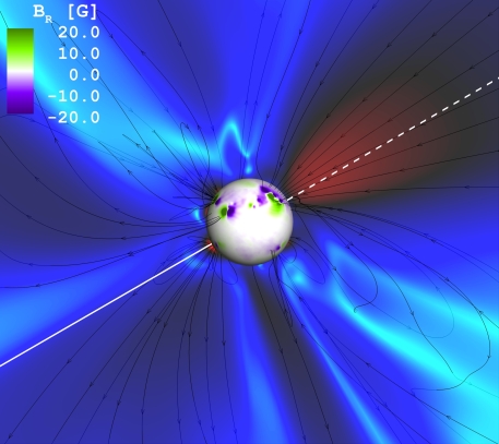
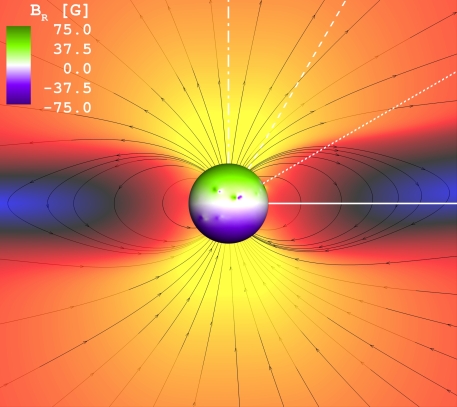
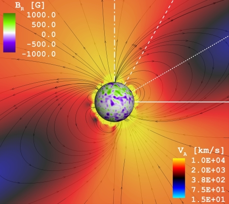
Figure 1: Meridional projection of the Alfvén speed ($V_{\rm A}$) in our AWSoM steady-state simulations. Top: Sun (CR 2107); Middle: Young Sun-like star (CR 2107 + 75 G large-scale dipole); Bottom: M-dwarf (Proxima Centauri). The sphere represents the stellar surface, color-coded by the radial field ($B_{\rm R}$) driving each model. The color scaling for $V_{\rm A}$ is preserved in all cases. The $V_{\rm A}$ profiles in Fig. 2 have been extracted along the white lines indicated. The field of view is 12 $R_{\bigstar}$ with a set of selected magnetic field lines in black.

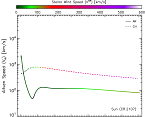
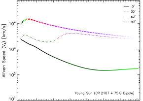
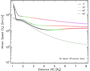
Figure 2: Radial profiles of $V_{\rm A}$ extracted from each of the AWSoM steady-state solutions (Fig. 1, white lines). Active Region (AR) and Coronal Hole (CH) profiles are included for the solar case (top panel). Four latitudes are probed in our two stellar cases (middle and bottom panels). The stellar wind speed ($V^{\rm SW}$) along each profile is indicated by the color-scale.

Table 1: Set of parameters assumed in the steady-state simulations using AWSoM.

Model	Magnetic Field	$\left<B\right>_{\rm S}$	$M_{\bigstar}$	$R_{\bigstar}$	$P_{\rm rot}$	$n_{0}$	$T_{0}$	$(S/B)_{\bigstar}$	$L_{\perp}\sqrt{B}$
	Distribution	[G]	[$M_{\odot}$]	[$R_{\odot}$]	[d]	[cm-3]	[K]	[W m-2 T-1]	[m $\sqrt{\text{T}}$]
Sun	CR 2107	3.0	1.0	1.0	25.38	2×10^10	5×10^4	1.1×10^6	1.5×10^5
Sun-like	CR 2107 + (75 G)^†	42.6	1.0	1.0	25.38	2×10^10$&5\times 10$	1.1×10^6	1.5×10^5
M-dwarf	Proxima Centauri^‡	448.8	0.122	0.155	83.0	2×10^10$&5\times 10$	1.1×10^6	6.0×10^5

From the AWSoM perspective, this could imply that additional modifications (apart from the surface magnetogram) to the boundary conditions might be required. However, as discussed by Sokolov et al. 2013, the scaling $(S/B)_{\bigstar}$ in the Alfv́en wave Poynting flux is consistent and equivalent to the magnetic to X-ray flux empirical relation of Pevtsov et al. (2003), which extends beyond the magnetic fluxes observed in M-dwarfs stars. For this reason, we retain the standard AWSoM value for this parameter in our Proxima Centauri simulations.

On the other hand, we consider the currently available information on M-dwarf stellar winds to adjust the normalization for the Alfvén wave correlation length $L_{\perp}\sqrt{B}$. Unfortunately, stellar wind properties in low mass stars (particularly M-dwarfs) are highly uncertain. Estimates of mass loss rates ($\dot{M}$) —interpreted as a measure of wind strength— are only available for 14 stellar systems (12 detections, 2 upper limits), of which only 3 are M-dwarfs (2 detections, 1 upper limit; see Wood 2018). For the particular case of Proxima Centauri, two different methods have been used to constrain the mass loss rate associated with its stellar wind. An upper limit of $\dot{\rm M}<0.2~{}\dot{\rm M}_{\odot}$ was placed by Wood et al. (2001), through the astrospheric signature in the Ly$\alpha$ line (Linsky & Wood 2014). A higher limit of $\dot{\rm M}<14$ $\dot{\rm M}_{\odot}$ was found by Wargelin & Drake (2002), measuring in X-rays the direct signature of charge exchange between the stellar wind ions and the local interstellar medium.

As the astrospheric method has been more commonly applied, we set $L_{\perp}\sqrt{B}=6.0\times 10^{5}$ m $\sqrt{\text{T}}$ which yields a stellar wind mass loss rate of $\dot{\rm M}\simeq 0.3$ $\dot{\rm M}_{\odot}$, which is still consistent with the Ly$\alpha$ limit (taking into account the typical errors of this technique; see Linsky & Wood 2014). This is the same $L_{\perp}\sqrt{B}$ value used in the stellar wind simulations of Proxima Centauri by Garraffo et al. (2016b), and Barnard’s Star by Alvarado-Gómez et al. (2019c). Finally, published stellar properties for this object are used in this case ($M_{\bigstar}=0.122$ $M_{\odot}$, $R_{\bigstar}=0.154$ $R_{\odot}$, $P_{\rm rot}=83.0$ d, Kiraga & Stepien 2007, Kervella et al. 2017, Collins et al. 2017). Table 2.1 contains a summary of all the parameters considered in our AWSoM steady-state simulations.

2.2 Flux-Rope CME Model

The Titov & Démoulin (TD, 1999) flux-rope eruption model is used to drive our M-dwarf CME simulations. In the SWMF implementation (e.g., Manchester et al. 2008, Jin et al. 2013), the twisted loop-like structure of the TD model is coupled to the AWSoM steady-state solution at the inner boundary (stellar surface), and initialized with eight different parameters related to the location (2), orientation, size (3), magnetic free energy ($E_{\rm B}^{\rm FR}$) and mass of the flux-rope ($M^{\rm FR}$). The CME simulations discussed here use the same parameters as in Alvarado-Gómez et al. (2019b), namely, longitude ($270$ deg), latitude ($36$ deg), tilt angle ($28$ deg), flux-tube radius ($20$ Mm), length ($\sim$ $150$ Mm), and loaded mass ($M^{\rm FR}=4.0\times~{}10^{14}$ g). We consider two values of $E_{\rm B}^{\rm FR}$ in order to probe the regimes of weak ($E_{\rm B,1}^{\rm FR}\simeq 4.1\times 10^{35}$ erg) and partial ($E_{\rm B,2}^{\rm FR}\simeq 2.0\times 10^{35}$ erg) large-scale magnetic CME confinement. Note that assuming a similar flare-CME magnetic energy partition as in the Sun (e.g., Emslie et al. 2012, Toriumi et al. 2017), our selected $E_{\rm B}^{\rm FR}$ values are consistent and sufficient to power the best CME candidate observed in Proxima Centauri so far ($F_{\rm X}\simeq 1.7\times 10^{31}$ erg, $E_{\rm K}^{\rm CME}\simeq 5\times 10^{31}$ erg; see Moschou et al. 2019). The initial parameters assumed in our TD flux-rope simulations are listed in Table 1.

Each CME simulation evolves for $90$ minutes (real time) from which we extract 3D snapshots of the entire simulation domain at a cadence of $1$ minute.

Table 1: Flux rope parameters initializing the TD CME simulations within the M-dwarf model.

Parameter	Value	Unit
Latitude	36.0	deg
Longitude	270.0	deg
Tilt angle†	28.0	deg
Radius ($R^{\rm FR}$)	20.0	Mm
Length ($L^{\rm FR}$)	150.0	Mm
Mass ($M^{\rm FR}$)	$4.0\times~{}10^{14}$	g
Magnetic energy ($E_{\rm B}^{\rm FR}$)	$4.1\times 10^{35}$	erg
	$2.0\times 10^{35}$

3 Results

3.1 Coronal Alfvén Speed Profiles

We examine first the coronal Alfvén speed distributions obtained in our steady-state solutions. Figure 1 compares the resulting $V_{\rm A}$ on an arbitrary meridional projection, with a common color scale saturated between $15$ km s^-1 $\leq V_{\rm A}\leq 10000$ km s^-1. Radial profiles for different regions/latitudes are indicated and correspondingly plotted in Fig. 2, together with the stellar wind speed ($V^{\rm SW}$) along the same profiles.

As expected, our simulated values of $V_{\rm A}$ for the Sun —which are consistent with observations (see Zucca et al. 2014)— are globally lower than their stellar counterparts (by up to one order of magnitude). The spatial distribution of $V_{\rm A}$ also follows the nominal behavior in the solar corona: large $V_{\rm A}$ values very close to active regions (strong small-scale field) and above coronal holes (low density sectors; see also Fig. 2, top panel). The lower $V_{\rm A}$ locations coincide with the high-density coronal streamers. Furthermore, the appearance of local minima in $V_{\rm A}$ above active regions, due to the superposition of the small- and large-scale solar magnetic field, is also captured in our simulation (see Mann et al. 2003).

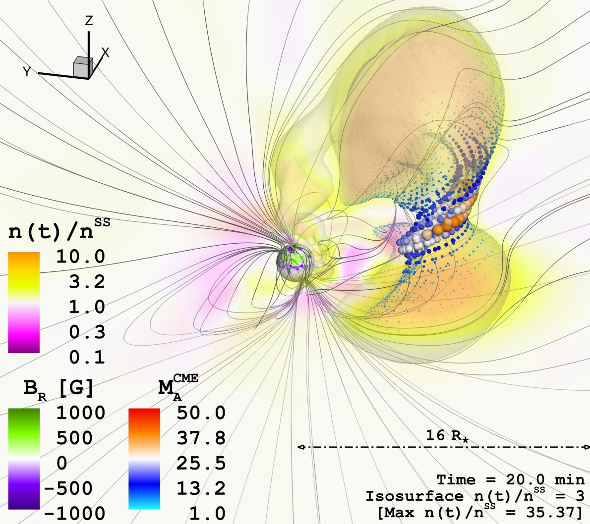
Figure 3: Snapshot during the temporal evolution of the weakly confined CME ($E_{\rm B,1}^{\rm FR}\simeq 4.1\times 10^{35}$ erg, $E_{\rm K,1}^{\rm CME}\simeq 1.7\times 10^{32}$ erg, $M_{1}^{\rm CME}\simeq 9.4\times 10^{15}$ g) within our M-dwarf simulation. The stellar surface is color coded (purple-green) by the radial magnetic field driving the ambient AWSoM solution. A secondary color scale (magenta-yellow) denotes the density contrast, $n(t)/n^{\rm SS}$, which is used to trace the CME front by the indicated iso-surface. The nominal shock condition, calculated from the Alfvénic Mach number of the CME front ($M_{\rm A}^{\rm CME}$, Eq. 1), is encoded simultaneously by the size of the scatter distribution (spheres) and by a tertiary color scale (cyan-red). The field of view is 32 $R_{\bigstar}$ with a set of selected large-scale magnetic field lines in gray.

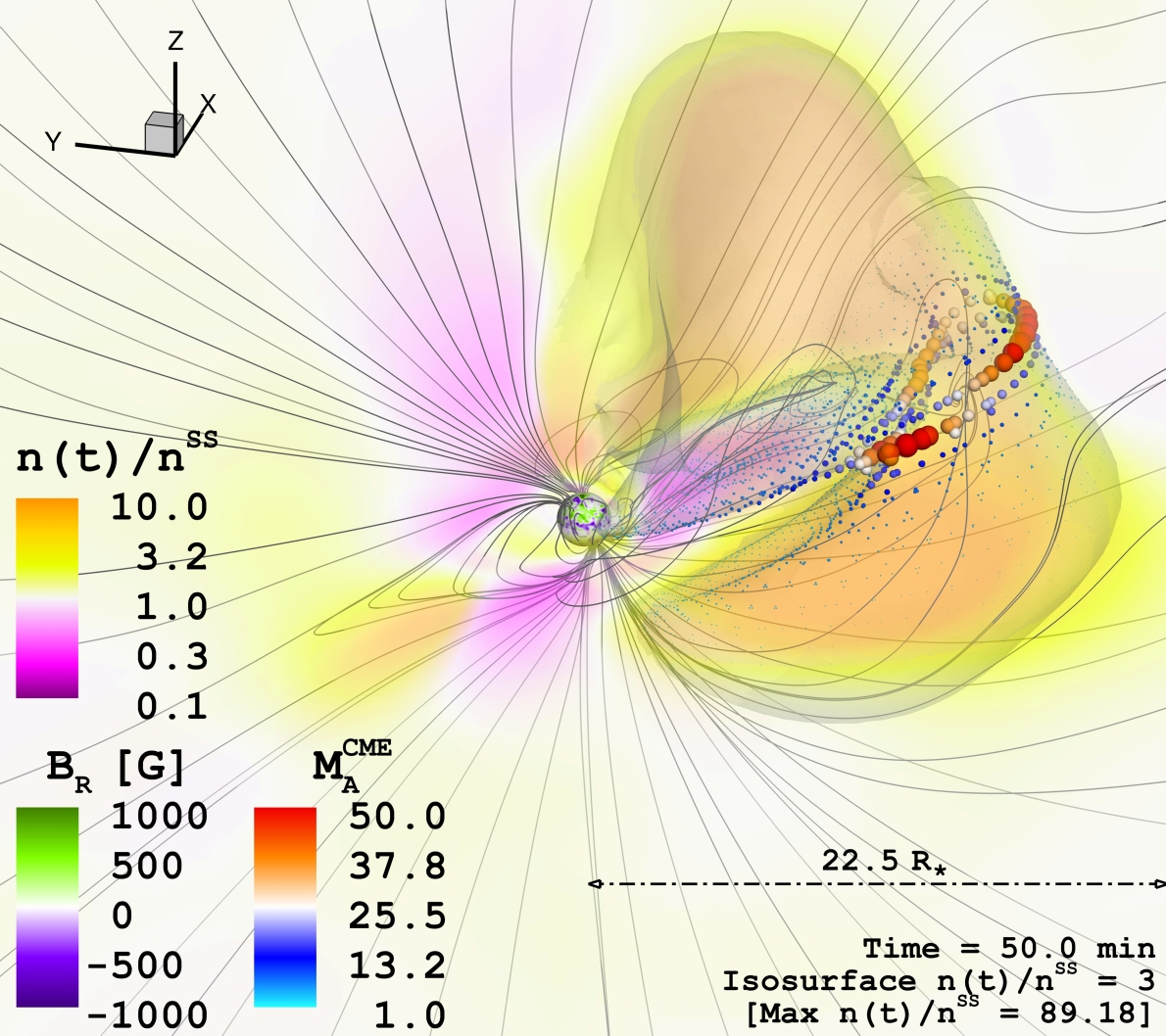
Figure 4: Snapshot during the temporal evolution of the partially confined CME ($E_{\rm B,2}^{\rm FR}\simeq 2.0\times 10^{35}$ erg, $E_{\rm K,2}^{\rm CME}\simeq 3.2\times 10^{31}$ erg, $M_{2}^{\rm CME}\simeq 4.0\times 10^{15}$ g) within our M-dwarf simulation. See caption of Fig. 3. Note the difference in field of view (45 $R_{\bigstar}$) and timestamp ($50$ min) in this case.

The influence from a stronger large-scale magnetic field can be clearly seen in the stellar $V_{\rm A}$ distributions (middle and bottom panels of Fig. 1). A dipolar geometry is established, with open-field magnetic polar regions showing large $V_{\rm A}$ values which gradually decrease towards the magnetic equator, where the density increases and the field strength decreases (see also Fig. 2, middle and bottom panels). Despite the large densities, the strong and ubiquitous small-scale field present in our M-dwarf model increases $V_{\rm A}$ close to the surface. As with the solar case, local minima in $V_{\rm A}$ occur at different positions and heights in the stellar corona. These are nearly absent in our Sun-like simulation, where the large-scale magnetic field dominates the surface distribution. As the large-scale field is weaker in the Sun-like case, $V_{\rm A}$ decays more rapidly with distance compared to the M-dwarf solution. Still, this is only true when evaluated on an equivalent latitude with respect to the large-scale magnetic field dipolar distribution.

Finally, it is worth noting that along the current sheet ($\sim 0^{\circ}$ in the Sun-like case, $\sim 30^{\circ}$ in the M-dwarf model), the Alfvén and stellar wind speeds are relatively small (i.e., $V_{\rm A}~{}<~{}1000$ km s^-1, $V^{\rm SW}~{}\leq~{}100$ km s^-1), whereas for other latitudes both quantities increase rapidly (particularly $V_{\rm A}$). As mentioned earlier, this will have important consequences on where in the stellar corona the conditions are more favorable for the escaping CMEs —or only certain regions of the expanding structure— to become super Alfvénic. This also clearly shows the importance of the geometry of the large-scale magnetic field and the need of 3D stellar wind/corona descriptions, neither of which are properly captured in simpler 1D, or even 2D rotationally symmetric, models. The importance the bimodal solar wind to the promotion of CME-driven shock formation has been shown in Manchester et al. (2005).

3.2 CME Evolution: Magnetic Suppression and Alfvénic Regimes

We now consider the results from the time-dependent CME simulations taking place in our Proxima-like corona and stellar wind environment. As mentioned earlier, two similar TD flux-rope eruptions, only differing by nearly a factor of $2$ in magnetic energy, serve to generate CME events in the regimes of weak (Fig. 3) and partial (Fig. 4) large-scale magnetic field confinement.

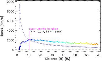
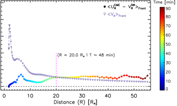
Figure 5: Global Alfvénic regimes as a function of distance in our simulated M-dwarf CME events (Left: weakly suppressed, Fig. 3; Right: partially suppressed, Fig. 4). In circles, and color-coded by simulation time, is the radial CME speed in the stellar wind frame $\left<U_{\rm R}^{\rm CME}-V_{\rm R}^{\rm SW}\right>$, spatially averaged over the expanding front. The mean Alfvén speed values $\left<V_{\rm A}\right>$, computed over the same spatial locations, are indicated by downward triangles. The nominal transition from sub-Alfvénic, $\left<M_{\rm A}^{\rm CME}\right><1$, to super-Alfvénic, $\left<M_{\rm A}^{\rm CME}\right>>1$, is indicated. The spike in speed at a distance of $\sim$$6.5~{}R_{\bigstar}$ in the right panel is due to the fragmentation of the CME, where the average speed is dominated by the outermost small fragments escaping the large-scale confinement (see Alvarado-Gómez et al. 2019a, 2019b).

Following Alvarado-Gómez et al. (2019b), we employ a density contrast $n(t)/n^{\rm SS}=3.0$ (with $n^{\rm SS}$ as the pre-eruption local density value) to identify and trace the CME front. We use the positions of each point on this time-evolving iso-surface to calculate the maximum radial velocity of the CME ($U_{\rm R}^{\rm CME}$), and to extract the steady-state pre-CME stellar wind ($V_{\rm R}^{\rm SW}$) and Alfvén ($V_{\rm A}$) speeds on the same locations in each time-step. As described before, this is necessary as the CME motion needs to be transformed to the stellar wind frame in order check the nominal Alfvén shock condition:

$$\dfrac{(U_{\rm R}^{\rm CME}-V_{\rm R}^{\rm SW})}{V_{\rm A}}\equiv M_{\rm A}^{\rm CME}>1\mbox{\,.}$$ (1)

Additionally, by integrating over the volume enclosed by the expanding front, taking into account the local escape velocity, we compute the mass ($M^{\rm CME}$) and kinetic energy ($E_{\rm K}^{\rm CME}$) of each CME event. This procedure yields $M_{1}^{\rm CME}\simeq 9.4\times 10^{15}$ g, $E_{\rm K,1}^{\rm CME}~{}\simeq~{}1.7\times 10^{32}$ erg for the weakly suppressed CME (Fig. 3), and a partially suppressed eruption with $M_{2}^{\rm CME}\simeq 4.0\times 10^{15}$ g, $E_{\rm K,2}^{\rm CME}\simeq 3.2\times 10^{31}$ erg (Fig. 4).

Figures 3 and 4 also include a visualization of the emerging shock regions through a distribution of spheres with size and color normalized by $M_{\rm A}^{\rm CME}$. Despite the difference in magnetic energy —and therefore in the confinement imposed by the large-scale field—  both events are able to generate shocks in the corona. As expected from the $V_{\rm A}$ distribution (Sect. 3.1), in both cases the super-Alfvénic region of the CME appears close to the current sheet. Relatively high $M_{\rm A}^{\rm CME}$ values appear locally (a few tens), much larger than in solar observations (see e.g. Maguire et al. 2020). Still, most of the perturbation front remains sub-Alfvénic as the eruption expands. These result uniquely depends on the 3D setup of the simulations and would not be found in a 1D case.

One significant difference between the simulated CME events appears in the height with respect to the stellar surface of the shock formation region (note that the field of view and timestamp in Figs 3 and 4 are different). All the other parameters of the TD flux-ropes being equal, this responds to the available magnetic energy to power the eruption, which in turn determines the relative importance of the magnetic suppression on the emerging eruption properties such as the CME speed (Alvarado-Gómez et al. 2018).

To better illustrate this, Fig. 5 shows averages over the CME front of the radial speed in the stellar wind frame $\left<U_{\rm R}^{\rm CME}-V_{\rm R}^{\rm SW}\right>$, and the local Alfvén speed $\left<V_{\rm A}\right>$, as a function of distance in both events. The resulting global behavior shows that the sub- to super-Alfvénic transition, indicative of the shock formation region, occurs at several stellar radii of height for both events (roughly at $10$ $R_{\bigstar}$ and $20$ $R_{\bigstar}$ for the events in Fig. 3 and 4, respectively). As discussed in the following section, this will have important consequences for any Type II bursts radio signatures induced by these shocks, and their detectability in the stellar regime with current instrumentation.

Finally, given the very large magnetic fields in the upper corona, temperature effects due to heating at radius $<10$ $R_{\bigstar}$ can be neglected. We have verified that along the current sheet in the M-dwarf simulation the wind temperature is $T<3$ MK. The resulting sound speed, for an hydrogen ideal gas, is $\sim 200$ km s${}^{-1}\ll V_{\rm A}$, so that the fast magnetosonic Mach number can be approximated with $M_{\rm A}^{\rm CME}$ within $<1\%$. Local larger temperature would push further out the distance of transition to super-Alfvénic CME speed by a modest amount.

4 Discussion

Solar type II radio bursts are typically divided by their associated wavelength or starting frequency (see Sharma & Mittal 2017 and references therein). Coronal type II radio bursts manifest at decimeter to metric wavelengths (MHz range), and interplanetary (IP) type II radio bursts appear at decametric to kilometric wavelengths (kHz range). One fundamental aspect related to their detection is the fact that the ionosphere impedes the transmission of radio waves with frequencies below $\sim$$10$ MHz (cutoff frequency). Therefore, only coronal type II bursts are accessible from ground-based instrumentation, which is also the sole possibility for their search in the context of stellar CMEs (see Villadsen 2017 and references therein).

The type II radio burst division is clearly motivated by the expected shock formation region. Still, several solar events display emission in the entire radio domain (m-to-km type II bursts). Gopalswamy et al. (2005) studied the properties of m-to-km type II radio bursts and their driving CMEs. This statistical analysis revealed that the majority of such radio events form close to the solar surface (i.e., below $3~{}R_{\odot}$ of height), and that the kinetic energy of the CME controls the life time of the radio emission (i.e., the range of frequencies covered by a given event). When the sample is restricted to coronal type II radio bursts alone, Gopalswamy et al. (2005) reports that the average shock formation region is even lower in height ($<2~{}R_{\odot}$; see also Ramesh et al. 2012, Gopalswamy et al. 2013).

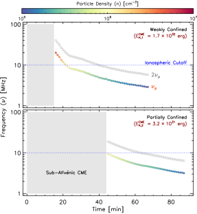
Figure 6: Temporal evolution of the expected type II radio burst frequencies associated with the shock regions in our simulated M-dwarf CMEs (Top: Weakly confined —Fig. 3; Bottom: Partially confined —Fig. 4). The fundamental ($\nu_{\rm p}\simeq 8980\sqrt{n}$ [Hz]) and first harmonic ($2\nu_{\rm p}$) of the plasma frequency are included. The associated $M_{\rm A}^{\rm CME}-$weighted mean plasma density is indicated by the color scale. Gray regions denote the intervals in which each CME is within the sub-Alfvénic regime (see Fig. 5).

Our analysis indicates that the shocks generated by the simulated M-dwarf CME events are pushed much farther out (see Fig. 5). At such distances, the coronal densities have decreased substantially compared to the standard formation region of solar type II bursts, shifting their frequencies close to, or below, the ionospheric cutoff. This is presented in Fig. 6, where the expected fundamental, $\nu_{\rm p}\simeq 8980\sqrt{n}$ [Hz], and first harmonic, $2\nu_{\rm p}$, of the plasma frequency are shown as a function of time. As regions with stronger shocks are expected to contribute more to the global type II emission, $M_{\rm A}^{\rm CME}-$weighted average densities are considered for this calculation.

Nevertheless, Fig. 6 shows that our simulated M-dwarf CMEs are not entirely radio-quiet. The expected fundamental and harmonic type II burst frequency drifts, generated by the strongest eruption considered here (Fig. 6, top panel), remain above the ionospheric cutoff for $\sim$ 10 min and $\sim$ 30 min, respectively. With approximately $\sim$ 80% less kinetic energy, only a $\sim$ 15 min harmonic lane clears this threshold in the weaker CME event (Fig. 6, bottom panel).

We now estimate whether such stellar type II radio bursts could be detected with ground-based instruments like the LOw Frequency ARray (LOFAR, van Haarlem et al. 2013). The strongest solar type II radio bursts reach spectral fluxes up to $10^{8}~{}\rm{Jy}$ (Schmidt & Cairns 2016). If we assume that this is also representative for M-dwarfs, that corresponds to $1.4~{}\rm{mJy}$ from Proxima Centauri’s distance of $1.3~{}\rm{pc}$, although this specific object in the Southern sky is not visible to LOFAR with a core location at a geographic latitude of 53 degrees North. LOFAR provides online tools for sensitivity estimates. For an observing frequency around $30~{}\rm{MHz}$, a maximum burst duration of $30~{}\rm{min}$, and a typical instantaneous burst bandwidth of $20~{}\rm{MHz}$ (Morosan et al. 2019), this leads to a sensitivity of just $5~{}\rm{mJy}$. And this number has to be treated with caution, since this estimate does not consider effects like calibration errors, ionospheric conditions, elevation of the source, and errors in beam models. The application of a factor of 5 is advised.

So it has to be concluded that even in the best case, i.e. harmonic emission from the weakly confined case in the upper panel of Fig. 6, with a total flux equal to the maximum solar value, CME-related type II radio burst emission cannot be observed by LOFAR even for the nearest M-dwarfs. The upcoming Square Kilometre Array (SKA), with its eponymous collecting area, could provide the necessary sensitivity and also geographic location for observations of Proxima Centauri. However, the lowest frequency band of SKA just starts at $50~{}\rm{MHz}$ (Nindos et al. 2019). From Fig. 6 it follows that there is no radio emission from frequencies above $50~{}\rm{MHz}$, as the sources of both fundamental and harmonic emission would be located in the region where the CME is still sub-Alfvénic.

In agreement with the results of Mullan & Paudel (2019), we find then that the ground-based detection of stellar CMEs via type II burst emission would be greatly hampered by the combined effect from magnetic suppression and large $V_{\rm A}$ values in the corona. It is worth noting that our Proxima Centauri background steady-state model already provides a best-case scenario: a lower bound on the mean surface field strength ($\sim\,$450 G; Reiners & Basri 2008), highest stellar wind density allowed by observations ($\dot{\rm M}\simeq 0.3$ $\dot{\rm M}_{\odot}$; Wood et al. 2001), and a CME shock trajectory following the current sheet (i.e., global minimum of $V_{\rm A}$ and low $V^{\rm SW}$; see bottom panels of Figs. 1 and 2). Still, our analysis shows that the required CME speed of $10$% the speed of light, suggested by Mullan & Paudel (2019) for Proxima-like surface magnetic fields, is overestimated. This most likely reflects the lower dimensionality and much simpler coronal model assumed in their study.

In terms of our simulated eruptions, the kinetic energies appear conservative with respect to the range determined for the best CME candidate observed in Proxima Centauri so far ($1\times 10^{29}$ erg $<E_{\rm K}^{\rm CME}<4\times 10^{34}$ erg; Moschou et al. 2019). Leaving aside considerations on occurrence rate, more energetic CMEs might be able to shock higher density regions closer to the stellar surface, increasing the radio frequency of the associated type II bursts. However, kinetic energies of CMEs appear correlated with small-scale surface magnetic flux in solar observations (e.g., Toriumi et al. 2017, Sindhuja & Gopalswamy 2020). If such a relation holds for stellar CMEs, it implies that $V_{\rm A}$ could also increase locally for stronger eruptions, creating again unfavorable conditions for the generation of shocks in the low corona. Still, this effect might be secondary for certain large-scale magnetic field strengths (i.e., reduced CME suppression). Future investigation will be pursued in this direction, expanding the parameter space to additional spectral types, surface magnetic field configurations, stellar wind properties, and CME eruption models.

5 Summary

Continuing our numerical investigation on stellar CMEs, we have considered here the expected connection between these eruptive phenomena and the generation of type II radio bursts.

Using physics-based 3D MHD corona and stellar wind models, we compared the Alfvén speed distribution for the Sun, a young Sun-like star, and a moderately active M-dwarf. We examined the regions where the Alfvén and stellar wind speeds provide the most favorable conditions for the generation of shocks in the corona. Furthermore, employing a state-of-the-art flux-rope eruption model, we simulated admissible CME events occurring in the archetypical star Proxima Centauri. We considered two eruptions representative of the regimes over which the ejected plasma is able to escape the large-scale magnetic field (weak and partial confinement). We showed that these eruptions are able to generate local strong shocks (i.e., high Alfvénic Mach number) in the vicinity of the astrospheric current sheet, which may lead to efficient acceleration of charged particles not due to magnetic reconnection.

The analysis of the global behavior in each CME event revealed that the shock formation region is pushed outwards compared to the average location observed in the Sun. From this, it follows that the associated type II radio burst frequencies would be shifted to lower values as the kinetic energy of the CME decreases. This poses a challenge for their detection from the ground, as in some cases their radio emission would lie very close to, or below, the ionospheric frequency cutoff. Nevertheless, extreme events might be able to more rapidly overcome the large-scale magnetic field suppression, decreasing the shock formation height and yielding amenable type II burst frequencies for current and future ground-based facilities.

References

- Alvarado-Gómez et al. (2018) Alvarado-Gómez, J. D., Drake, J. J., Cohen, O., Moschou, S. P., & Garraffo, C. 2018, ApJ, 862, 93
- Alvarado-Gómez et al. (2019a) Alvarado-Gómez, J. D., Drake, J. J., Garraffo, C., et al. 2019a, arXiv e-prints, arXiv:1912.12314
- Alvarado-Gómez et al. (2019b) Alvarado-Gómez, J. D., Drake, J. J., Moschou, S. P., et al. 2019b, ApJ, 884, L13
- Alvarado-Gómez et al. (2019c) Alvarado-Gómez, J. D., Garraffo, C., Drake, J. J., et al. 2019c, ApJ, 875, L12
- Argiroffi et al. (2019) Argiroffi, C., Reale, F., Drake, J. J., et al. 2019, Nature Astronomy, 328
- Benz (2017) Benz, A. O. 2017, Living Reviews in Solar Physics, 14, 2
- Bilenko (2018) Bilenko, I. A. 2018, Geomagnetism and Aeronomy, 58, 989
- Cairns et al. (2003) Cairns, I. H., Knock, S. A., Robinson, P. A., & Kuncic, Z. 2003, Space Sci. Rev., 107, 27
- Caramazza et al. (2007) Caramazza, M., Flaccomio, E., Micela, G., et al. 2007, A&A, 471, 645
- Cherenkov et al. (2017) Cherenkov, A., Bisikalo, D., Fossati, L., & Möstl, C. 2017, ApJ, 846, doi:10.3847/1538-4357/aa82b2
- Cohen et al. (2017) Cohen, O., Yadav, R., Garraffo, C., et al. 2017, ApJ, 834, 14
- Collins et al. (2017) Collins, J. M., Jones, H. R. A., & Barnes, J. R. 2017, A&A, 602, A48
- Compagnino et al. (2017) Compagnino, A., Romano, P., & Zuccarello, F. 2017, Sol. Phys., 292, 5
- Cranmer (2017) Cranmer, S. R. 2017, ApJ, 840, 114
- Crosley & Osten (2018a) Crosley, M. K., & Osten, R. A. 2018a, ApJ, 856, doi:10.3847/1538-4357/aaaec2
- Crosley & Osten (2018b) —. 2018b, ApJ, 862, 113
- Crosley et al. (2016) Crosley, M. K., Osten, R. A., Broderick, J. W., et al. 2016, ApJ, 830, 24
- Davenport (2016) Davenport, J. R. A. 2016, ApJ, 829, 23
- Davenport et al. (2019) Davenport, J. R. A., Covey, K. R., Clarke, R. W., et al. 2019, ApJ, 871, 241
- DeRosa & Barnes (2018) DeRosa, M. L., & Barnes, G. 2018, ApJ, 861, 131
- Donati (2011) Donati, J.-F. 2011, in IAU Symposium, Vol. 271, Astrophysical Dynamics: From Stars to Galaxies, ed. N. H. Brummell, A. S. Brun, M. S. Miesch, & Y. Ponty, 23–31
- Drake et al. (2016) Drake, J. J., Cohen, O., Garraffo, C., & Kashyap, V. 2016, in IAU Symposium, Vol. 320, Solar and Stellar Flares and their Effects on Planets, ed. A. G. Kosovichev, S. L. Hawley, & P. Heinzel, 196–201
- Drake et al. (2013) Drake, J. J., Cohen, O., Yashiro, S., & Gopalswamy, N. 2013, ApJ, 764, 170
- Emslie et al. (2012) Emslie, A. G., Dennis, B. R., Shih, A. Y., et al. 2012, ApJ, 759, 71
- Fraschetti et al. (2018) Fraschetti, F., Drake, J. J., Cohen, O., & Garraffo, C. 2018, ApJ, 853, 112
- Garraffo et al. (2016a) Garraffo, C., Drake, J. J., & Cohen, O. 2016a, A&A, 595, A110
- Garraffo et al. (2016b) —. 2016b, ApJ, 833, L4
- Glassgold et al. (1997) Glassgold, A. E., Najita, J., & Igea, J. 1997, ApJ, 480, 344
- Gombosi et al. (2018) Gombosi, T. I., van der Holst, B., Manchester, W. B., & Sokolov, I. V. 2018, Living Reviews in Solar Physics, 15, 4
- Gopalswamy et al. (2005) Gopalswamy, N., Aguilar-Rodriguez, E., Yashiro, S., et al. 2005, Journal of Geophysical Research (Space Physics), 110, A12S07
- Gopalswamy et al. (2019) Gopalswamy, N., Mäkelä, P., & Yashiro, S. 2019, arXiv e-prints, arXiv:1912.07370
- Gopalswamy et al. (2009) Gopalswamy, N., Thompson, W. T., Davila, J. M., et al. 2009, Sol. Phys., 259, 227
- Gopalswamy et al. (2013) Gopalswamy, N., Xie, H., Mäkelä, P., et al. 2013, Advances in Space Research, 51, 1981
- Guarcello et al. (2019) Guarcello, M. G., Micela, G., Sciortino, S., et al. 2019, A&A, 622, A210
- Ilin et al. (2019) Ilin, E., Schmidt, S. J., Davenport, J. R. A., & Strassmeier, K. G. 2019, A&A, 622, A133
- Jeffers et al. (2017) Jeffers, S. V., Boro Saikia, S., Barnes, J. R., et al. 2017, MNRAS, 471, L96
- Jeffers et al. (2014) Jeffers, S. V., Petit, P., Marsden, S. C., et al. 2014, A&A, 569, A79
- Jin et al. (2017a) Jin, M., Manchester, W. B., van der Holst, B., et al. 2017a, ApJ, 834, 172
- Jin et al. (2013) —. 2013, ApJ, 773, 50
- Jin et al. (2017b) —. 2017b, ApJ, 834, 173
- Kashyap et al. (2002) Kashyap, V. L., Drake, J. J., Güdel, M., & Audard, M. 2002, ApJ, 580, 1118
- Kervella et al. (2017) Kervella, P., Thévenin, F., & Lovis, C. 2017, A&A, 598, L7
- Kiraga & Stepien (2007) Kiraga, M., & Stepien, K. 2007, Acta Astron., 57, 149
- Kundu (1965) Kundu, M. R. 1965, Solar radio astronomy
- Lammer (2013) Lammer, H. 2013, Origin and Evolution of Planetary Atmospheres (Springer Berlin Heidelberg), doi:10.1007/978-3-642-32087-3
- Linsky & Wood (2014) Linsky, J. L., & Wood, B. E. 2014, ASTRA Proceedings, 1, 43
- Liu et al. (2016) Liu, L., Wang, Y., Wang, J., et al. 2016, ApJ, 826, 119
- Loyd et al. (2018) Loyd, R. O. P., France, K., Youngblood, A., et al. 2018, ApJ, 867, 71
- Maguire et al. (2020) Maguire, C. A., Carley, E. P., McCauley, J., & Gallagher, P. T. 2020, A&A, 633, A56
- Manchester et al. (2005) Manchester, W. B., I., Gombosi, T. I., De Zeeuw, D. L., et al. 2005, ApJ, 622, 1225
- Manchester et al. (2008) Manchester, IV, W. B., Vourlidas, A., Tóth, G., et al. 2008, ApJ, 684, 1448
- Mann et al. (2003) Mann, G., Klassen, A., Aurass, H., & Classen, H. T. 2003, A&A, 400, 329
- Micela (2018) Micela, G. 2018, Stellar Coronal Activity and Its Impact on Planets (Springer International Publishing AG), 19
- Morgenthaler et al. (2012) Morgenthaler, A., Petit, P., Saar, S., et al. 2012, A&A, 540, A138
- Morosan et al. (2019) Morosan, D. E., Carley, E. P., Hayes, L. A., et al. 2019, Nature Astronomy, 3, 452
- Moschou et al. (2017) Moschou, S.-P., Drake, J. J., Cohen, O., Alvarado-Gomez, J. D., & Garraffo, C. 2017, ApJ, 850, 191
- Moschou et al. (2019) Moschou, S.-P., Drake, J. J., Cohen, O., et al. 2019, ApJ, 877, 105
- Mullan & Bais (2018) Mullan, D. J., & Bais, H. P. 2018, ApJ, 865, 101
- Mullan & Paudel (2019) Mullan, D. J., & Paudel, R. R. 2019, ApJ, 873, 1
- Nindos et al. (2019) Nindos, A., Kontar, E. P., & Oberoi, D. 2019, Advances in Space Research, 63, 1404
- Nutzman & Charbonneau (2008) Nutzman, P., & Charbonneau, D. 2008, PASP, 120, 317
- Odert et al. (2017) Odert, P., Leitzinger, M., Hanslmeier, A., & Lammer, H. 2017, MNRAS, 472, 876
- Oran et al. (2017) Oran, R., Landi, E., van der Holst, B., Sokolov, I. V., & Gombosi, T. I. 2017, ApJ, 845, 98
- Osten (2016) Osten, R. 2016, Solar explosive activity throughout the evolution of the solar system, 23–55
- Osten & Wolk (2017) Osten, R. A., & Wolk, S. J. 2017, in IAU Symposium, Vol. 328, Living Around Active Stars, ed. D. Nandy, A. Valio, & P. Petit, 243–251
- Pevtsov et al. (2003) Pevtsov, A. A., Fisher, G. H., Acton, L. W., et al. 2003, ApJ, 598, 1387
- Pick et al. (2006) Pick, M., Forbes, T. G., Mann, G., et al. 2006, Multi-Wavelength Observations of CMEs and Associated Phenomena, Vol. 21 (Kluwer Academic Publishers), 341
- Powell et al. (1999) Powell, K. G., Roe, P. L., Linde, T. J., Gombosi, T. I., & De Zeeuw, D. L. 1999, Journal of Computational Physics, 154, 284
- Ramesh et al. (2012) Ramesh, R., Lakshmi, M. A., Kathiravan, C., Gopalswamy, N., & Umapathy, S. 2012, ApJ, 752, 107
- Reiners (2014) Reiners, A. 2014, in IAU Symposium, Vol. 302, Magnetic Fields throughout Stellar Evolution, ed. P. Petit, M. Jardine, & H. C. Spruit, 156–163
- Reiners & Basri (2008) Reiners, A., & Basri, G. 2008, A&A, 489, L45
- Sachdeva et al. (2019) Sachdeva, N., van der Holst, B., Manchester, W. B., et al. 2019, ApJ, 887, 83
- Schmidt & Cairns (2016) Schmidt, J. M., & Cairns, I. H. 2016, Geophys. Res. Lett., 43, 50
- Segura et al. (2010) Segura, A., Walkowicz, L. M., Meadows, V., Kasting, J., & Hawley, S. 2010, Astrobiology, 10, 751
- Sharma & Mittal (2017) Sharma, J., & Mittal, N. 2017, Astrophysics, 60, 213
- Shibayama et al. (2013) Shibayama, T., Maehara, H., Notsu, S., et al. 2013, The Astrophysical Journal Supplement Series, 209, doi:10.1088/0067-0049/209/1/5
- Shulyak et al. (2019) Shulyak, D., Reiners, A., Nagel, E., et al. 2019, A&A, 626, A86
- Sindhuja & Gopalswamy (2020) Sindhuja, G., & Gopalswamy, N. 2020, ApJ, 889, 104
- Sokolov et al. (2013) Sokolov, I. V., van der Holst, B., Oran, R., et al. 2013, ApJ, 764, 23
- Sun et al. (2015) Sun, X., Bobra, M. G., Hoeksema, J. T., et al. 2015, ApJ, 804, L28
- Thalmann et al. (2015) Thalmann, J. K., Su, Y., Temmer, M., & Veronig, A. M. 2015, ApJ, 801, L23
- Thalmann et al. (2017) —. 2017, ApJ, 844, L27
- Tilley et al. (2019) Tilley, M. A., Segura, A., Meadows, V., Hawley, S., & Davenport, J. 2019, Astrobiology, 19, 64
- Titov & Démoulin (1999) Titov, V. S., & Démoulin, P. 1999, A&A, 351, 707
- Toriumi et al. (2017) Toriumi, S., Schrijver, C. J., Harra, L. K., Hudson, H., & Nagashima, K. 2017, ApJ, 834, 56
- Tóth et al. (2012) Tóth, G., van der Holst, B., Sokolov, I. V., et al. 2012, Journal of Computational Physics, 231, 870
- Tuomi et al. (2019) Tuomi, M., Jones, H. R. A., Anglada-Escudé, G., et al. 2019, arXiv e-prints, arXiv:1906.04644
- Turner & Drake (2009) Turner, N. J., & Drake, J. F. 2009, ApJ, 703, 2152
- van der Holst et al. (2019) van der Holst, B., Manchester, W. B., I., Klein, K. G., & Kasper, J. C. 2019, ApJ, 872, L18
- van der Holst et al. (2014) van der Holst, B., Sokolov, I. V., Meng, X., et al. 2014, ApJ, 782, 81
- van Haarlem et al. (2013) van Haarlem, M. P., Wise, M. W., Gunst, A. W., et al. 2013, A&A, 556, A2
- Vida et al. (2019) Vida, K., Leitzinger, M., Kriskovics, L., et al. 2019, A&A, 623, A49
- Vidotto et al. (2014) Vidotto, A. A., Jardine, M., Morin, J., et al. 2014, MNRAS, 438, 1162
- Villadsen & Hallinan (2019) Villadsen, J., & Hallinan, G. 2019, ApJ, 871, 214
- Villadsen (2017) Villadsen, J. R. 2017, PhD thesis, California Institute of Technology
- Wargelin & Drake (2002) Wargelin, B. J., & Drake, J. J. 2002, ApJ, 578, 503
- Webb & Howard (2012) Webb, D. F., & Howard, T. A. 2012, Living Reviews in Solar Physics, 9, doi:10.12942/lrsp-2012-3
- Wild & McCready (1950) Wild, J. P., & McCready, L. L. 1950, Australian Journal of Scientific Research A Physical Sciences, 3, 387
- Wood (2018) Wood, B. E. 2018, in Journal of Physics Conference Series, Vol. 1100, Journal of Physics Conference Series, 012028
- Wood et al. (2001) Wood, B. E., Linsky, J. L., Müller, H.-R., & Zank, G. P. 2001, ApJ, 547, L49
- Wood et al. (2005) Wood, B. E., Müller, H.-R., Zank, G. P., Linsky, J. L., & Redfield, S. 2005, ApJ, 628, L143
- Yadav et al. (2016) Yadav, R. K., Christensen, U. R., Wolk, S. J., & Poppenhaeger, K. 2016, ApJ, 833, L28
- Yashiro & Gopalswamy (2009) Yashiro, S., & Gopalswamy, N. 2009, in IAU Symposium, Vol. 257, Universal Heliophysical Processes, ed. N. Gopalswamy & D. F. Webb, 233–243
- Yiǧit (2018) Yiǧit, E. 2018, Atmospheric and Space Sciences: Ionospheres and Plasma Environments, Vol. 2, doi:10.1007/978-3-319-62006-0
- Zucca et al. (2014) Zucca, P., Carley, E. P., Bloomfield, D. S., & Gallagher, P. T. 2014, A&A, 564, A47