In-Machine-Learning Database:
Reimagining Deep Learning with Old-School SQL

Abstract

In-database machine learning has been very popular, almost being a cliche. However, can we do it the other way around? In this work, we say “yes” by applying plain old SQL to deep learning, in a sense implementing deep learning algorithms with SQL.

Most deep learning frameworks, as well as generic machine learning ones, share a de facto standard of multidimensional array operations, underneath fancier infrastructure such as automatic differentiation. As SQL tables can be regarded as generalisations of (multi-dimensional) arrays, we have found a way to express common deep learning operations in SQL, encouraging a different way of thinking and thus potentially novel models. In particular, one of the latest trend in deep learning was the introduction of sparsity in the name of graph convolutional networks, whereas we take sparsity almost for granted in the database world.

As both databases and machine learning involve transformation of datasets, we hope this work can inspire further works utilizing the large body of existing wisdom, algorithms and technologies in the database field to advance the state of the art in machine learning, rather than merely integerating machine learning into databases.

1 Introduction

Both machine learning and databases obviously involve transformation of (or computation over) collections of numbers. Combining the two fields is then an obvious conclusion. But the way of such fusion seems to have been unilateral. Much more effort has been spent towards providing machine learning capabilities in a database context, or so-called “In-Database Machine Learning” [18], compared to integeration in the opposite direction, which we call “In-Machine-Learning Database”.

We speculate that the connotation of databases has been more towards “systems” than towards algorithms, compared to that of machine learning, making it seemingly more natural to apply the latter to the former. Modern machine learning, in particular deep learning, has been growing into expansive software systems as well, which suggests us to seriously consider the reverse.

In this work we get back at the basic (or not so basic) notion of “transforming collections of numbers” and try substituting the typical operations in machine learning with the most prominent tool in databases, i.e. SQL, to see whatever novel we can find under this different perspective.

2 Related Work

In this section, we review some representative works connecting the two fields of machine learning (in particular, deep learning) and databases, so that we can position this work properly in the whole data science landscape. In particular, reviewing these works helps us with a bird’s-eye view of why the relational model, having been ubiquitous in databases since the beginning of the field, should still interest those at the tip of deep learning research.

2.1 Machine Learning in Databases

MADlib [10] is probably the apex of the classical approach where machine learning subroutines are provided as black-boxes in SQL. MADlib also focuses on conventional machine learning rather than deep learning.

SciDB [30, 29] substitutes relational tables with multidimensional arrays. In-database linear algebra and analytics can then be added, resulting in a crossover between a numerical library and a database.

Tensor-Relational Model [14] is an elaborated treatise on the role of multidimensional arrays in relational databases.

MLog [18] provides a domain-specific language designed for deep learning. The MLog language is integerated into RDBMS by mixing with SQL. It operates on multidimensional arrays (tensors) rather than relational tables. The implementation compiles MLog into TensorFlow[1] programs.

In [25], array operations, automatic differentiation and gradient descent are implemented via SQL extensions.

[33] envisioned some possible ways to enhance database functionality with deep learning, beyond ease of access of deep learning in databases.

A strong argument favouring in-database machine learning is that databases are often mature distributed systems, so distributed machine learning would supposedly require little extra effort on the user in a database setting. [20] explores such a setting.

2.2 Database Functionality in General Machine Learning Settings

Despite claimed as “an in-database framework”, AIDA [5, 4] provides a client interface to a SQL server in the Python language, which is the de facto standard in the machine learning world, AIDA also shifts some of the computation to the server side, or more precisely, a Python interpreter embedded in the database server. So AIDA is best understood as implementing (low-level computation of) machine learning in a database, and then providing the augmented database to machine learning to the user.

ML2SQL [26, 27] compiles a unified declarative domain-specific language to both database operations in SQL and ML-style array operations in python.

SystemML [3] and its successor SystemDS [2] also provide a unified language, but they use non-relational databases.

TensorLog [12] implements probabilistic logic, essential to probabilistic databases, over typical deep learning infrastructure.

In addition to machine learning in databases, [33] also envisions providing system-level facilities and distributed computation developed in the database community to deep learning.

Finally, the Pandas [19] library familiar to data scientist already provides some essential relational functionalities such as JOIN and SELECT.

2.3 Neural Networks Designed for Relational Models

There are also neural networks specifically designed for learning relations. [32] summerizes very well the effort in this regard before the ”deep learning takeover”, including Graph Neural Networks (GNN) [23], and Relational Neural Networks [31].

In the more recent surge of deep learning, [22] explores a general deep learning architecture whose outputs are relations, with applications to understanding scenes. [21] combines relational reasoning with recurrent neural networks. [35] further applies the architecture in [22] to complex reinforcement learning tasks. [13] employs a modified logistic regression over hidden layers to learn relations. Lifted Relational Neural Networks [28] combines first-order logic with neural networks to learn relational structures.

Note that all of these models designed to learn relations, while worth mentioning, overlap little with our claim that relational-model-based SQL can be used as building blocks for general deep learning.

2.4 Relational Models versus Graph Convolutional Networks

Even being the ”fanciest of the fanciest” topic in Machine Learning, Graph convolutional network [16] (GCN) can’t escape the link to relational models [24]. [22] advocates relating relational models and graph convolutional networks, as well as deep learning in general, with extensive review.

One interesting fact about GCNs is that GPUs no longer make the usual vast speedups. Even without consideration of relations, GPUs failed to accelerate beyond one order of magnitude [16]. We speculate that it is something inherent given the underlying sparsity, posing the same challenge to deep learning and databases alike.

Apparently, edges of graphs are relations. But relations are not always edges – they could be hyperedges! From the point of view of the “ relational” people, it is really a no-brainer that we could have hypergraph variants of GCNs. [7] discusses them without addressing relational models while [34] and [11] address both relational models and hypergraph neural networks.

3 Architecture

In this part, we give a big picture of our proposed way of doing deep learning with SQL. While the meaning of deep learning may not be exact enough to prevent intentionally creating a counterexample to our arguments, actual instances of deep learning almost universally follow the structures described here, at least in a practical, computational sense.

3.1 The (Usual) Way of Deep learning

A deep learning model can usually be regarded as a scalar function $\mathcal{f}(\mathcal{D},\mathcal{P})$, where $\mathcal{D}$ denotes a set of inputs (data) and $\mathcal{P}$ denotes the model parameters. Our hypothetic goal is to find

$$\operatorname*{argmin}\limits_{\mathcal{P}}\mathcal{f}(\mathcal{D}_{0},\mathcal{P})$$

where $\mathcal{D}_{0}$ can be interpreted as either the set of all possible inputs or a test set.

The global minimization is usually intractable. So the learning process involves some iterative optimization involving the gradients $\dfrac{\partial\mathcal{f}(\mathcal{D},\mathcal{P})}{\partial\mathcal{P}}$. The iterative optimization takes the steps shown in Algorithm 1.

Load training set as $\mathcal{D}$ ;

Randomly initialize $\mathcal{P}$ ;

while not meeting stopping criteria do

       (1) Evaluate $\mathcal{f}(\mathcal{D},\mathcal{P})$ ;

       (2) Evaluate $\dfrac{\partial\mathcal{f}(\mathcal{D},\mathcal{P})}{\partial\mathcal{P}}$ (taken care of by automatic differentiation; not necessarily mathematically precise) ;

       (3) Update $\mathcal{P}$ with a new value computed with the old $\mathcal{P}$ and $\dfrac{\partial\mathcal{f}(\mathcal{D},\mathcal{P})}{\partial\mathcal{P}}$ (may carry over state from previous iterations) ;

      

end while

Algorithm 1 Typical deep learning control flow

This is the most basic pattern. Some deep learning algorithms follow alternative versions. In real world scenarios, it is often only possible to train with stochastic gradient descent which follows the general pattern outlined in Algorithm 2, where only a subset of $\mathcal{D}$ is picked for training each iteration.

Load $\mathcal{D}$ ; Initialize $\mathcal{P}$ ;

while not meeting stopping criteria do

       (1) Evaluate $\mathcal{f}(\mathcal{D}^{\prime},\mathcal{P})$ where $\mathcal{D}^{\prime}\in\mathcal{D}$ (chosen per iteration) ;

       (2) Evaluate $\dfrac{\partial\mathcal{f}(\mathcal{D},\mathcal{P})}{\partial\mathcal{P}}$ ;

       (3) Update $\mathcal{P}$ ;

      

end while

Algorithm 2 Deep learning control flow that stochastic gradient descent uses

A recurrent neural network predicting the next symbol given a prefix would be trained with Algorithm 3, in a self-supervised fashion, where the samples are encoded one megasequence of vectors $\mathcal{S}$.

Load $\mathcal{S}$ ; Initialize $\mathcal{P}$ ;

while not meeting stopping criteria do

       (1) Evaluate $\mathcal{f}(\mathcal{S},\mathcal{P})$:

       (1a) Initialize hidden states $\mathcal{H}$ ( typically with zeroes );

       (1b) for  $\mathcal{S}^{\prime}$ (embeddings of) sub-sequence of $\mathcal{S}$  do

             (1b1) Evaluate network output (embeddings of predicted sub-sequence) $\mathcal{S}^{\prime\prime}$ and update hidden states $\mathcal{H}$ with $(\mathcal{S}^{\prime\prime},\mathcal{H})\leftarrow f_{1}(S^{\prime},\mathcal{H},\mathcal{P})$ ;

             (1b2) Evaluate per-sub-sequence loss $f_{2}(\mathcal{S}^{\prime\prime},\mathcal{S})$ by comparing prediction $\mathcal{S}^{\prime\prime}$ and the corresponding (embeddings of) sub-sequence of $\mathcal{S}$ ;

            

       end for

       (1c) compute total loss $\mathcal{f}(\mathcal{S},\mathcal{P})$ by summing or averaging all per-sub-sequence losses ;

       (2) Evaluate $\dfrac{\partial\mathcal{f}(\mathcal{S},\mathcal{P})}{\partial\mathcal{P}}$ ;

       (3) Update $\mathcal{P}$ ;

      

end while

Algorithm 3 Control flow for training recurrent neural networks

Even unconventional uses of deep learning are not so unconventional in terms of control flows. Neural style transfer [8] follows the pattern in Algorithm 4, essentially just switching the argument in Algorithm 1 from $\mathcal{P}$ to $\mathcal{D}$.

Load content image $\mathcal{I}^{\prime}$ and style image $\mathcal{I}^{\prime\prime}$ ;

Initialize image $\mathcal{I}$ ( maybe randomly but usually $\mathcal{I}\leftarrow\mathcal{I}^{\prime}$);

Load (pre-trained) $\mathcal{P}$ ;

while not meeting stopping criteria do

       (1) Evaluate $\mathcal{f}(\mathcal{I},\mathcal{I}^{\prime},\mathcal{I}^{\prime\prime},\mathcal{P})$ ;

       (2) Evaluate $\dfrac{\partial\mathcal{f}(\mathcal{I},\mathcal{P})}{\partial\mathcal{I}}$ ;

       (3) Update $\mathcal{I}$ ;

      

end while

Algorithm 4 Control flow for neural style transfer

Note that the content image $\mathcal{I}^{\prime}$ and style image $\mathcal{I}^{\prime\prime}$ are never modified once loaded. In practice, it is often possible to leave out $\mathcal{I}^{\prime}$ in the iterative optimization altogether so long as $\mathcal{I}^{\prime}$ is used as the initial value of $\mathcal{I}$ [6]. Adversial example generation, like fast gradient sign attack [9], works in a very similar way by perturbing $\mathcal{D}$ to maximize $\mathcal{f}(\mathcal{D},\mathcal{P})$ in Algorithm 1 rather than perturbing $\mathcal{P}$ to minimize it. The phenomenal generative adversarial network (GAN) pipes two ordinary networks with parameter sets $\mathcal{P}_{1}$ and $\mathcal{P}_{2}$ together and run two optimizations in lockstep as shown in Algorithm 5.

Initialize $\mathcal{P}_{1}$, $\mathcal{P}_{2}$;

Load true samples $\mathcal{D}$;

while not meeting stopping criteria do

       (1) Evaluate $\mathcal{f}(\mathcal{D},\mathcal{N},\mathcal{P}_{1},\mathcal{P}_{2})=f_{2}(\mathcal{D},f_{1}(\mathcal{N},\mathcal{P}_{1}),\mathcal{P}_{2})$ where $\mathcal{N}$ is some kind of noise ;

       (2) Evaluate $\dfrac{\partial\mathcal{f}(\mathcal{D},\mathcal{N},\mathcal{P}_{1},\mathcal{P}_{2})}{\partial\mathcal{P}_{1}}$ and $\dfrac{\partial\mathcal{f}(\mathcal{D},\mathcal{N},\mathcal{P}_{1},\mathcal{P}_{2})}{\partial\mathcal{P}_{2}}$ ;

       (3) Update $\mathcal{P}_{1}$ (maximizing) and $\mathcal{P}_{2}$ (minimizing)

       according to respective gradients;

      

end while

Algorithm 5 Control flow for generative adversarial networks

Function $f_{1}$ along with parameters $\mathcal{P}_{1}$ is the so-called generator network producing “fake” samples given noise as input, while the discriminator network with parameters $\mathcal{P}_{2}$ trying work out a score for each of both these “fake” samples and the “real” ones given as the training set. Then, one number representing how well the scores separate the two types of samples is summarized from the scores. Finally the two sets of parameters are optimized with respect to this number, albeit with opposite signs. Surely the order of steps (2) and (3) does not matter.

While there could be other ways to code a deep learning program, the pattern is quite clear. The control flows of deep learning programs are relatively simple, whereas the bulk of the effort are distributed to the design of the models, manifesting primarily in Step (1) of each example, among the 3 major steps conveniently partitioned out of the main loops.

As for Step (2) and (3), there is a separation of concern here. Pragmatically, a major breakthrough that enabled the explosive progress of deep learning is the automatic differentiation. While still an active field of research, development of new deep learning models can be separated from studying automatic differentiation (Step (2)) itself. We can mix and match different flavors of control flows with different optimization algorithms, or more precisely, different update strategies (Step (3)). While some combinations work better than others, in general inventors of new deep learning models do not concern themselves with which update strategy to pick until tuning the performance of the model.

3.2 Tensor to Relations and back again

Modern deep learning infrastructure has been almost universally built upon array-oriented programming paradigms. In this work, we concern ourselves with expressing the deep learning model $\mathcal{f}$ in (a very limited set of) SQL.

4 DL-in-SQL by Examples

While we are far from a formal proof that SQL can express every possible deep learning model because of the obvious lack of precise definition of the latter, we nevertheless demonstrate how the bread-and-butter constructs of deep learning can be expressed in SQL.

Here, we use an example deep learning task in stark contrast to typical database-related ones, to demonstrate that our architechture is really geared towards deep learning in general. We will introduce how frequent layers can be cast into SQL along the way. Without further ado, we begin the demonstration.

4.1 Image Classifier Convolutional Networks

In this example, we demonstrate how to specify a convolutional neural network for computer vision in SQL. The model takes $N$ sample images together as input, where $N$ varies depending on how the model is used. The model is fixed for 10 classes, and $32\times 32$ RGB images. Computationally, the neural network displays the structure illustrated in Figure 1. To make things crystal clear, we have drawn all parameters of the network explicitly, so each “step of computation” in a box does not contain any states. This is quite different from many illustrations found elsewhere. For instance, in deep learning jargon, the first “convolutional layer” would conceptually include both “conv1” in the box and the two parameter arrays (kernel and biases) marked in blue, usually not shown explicitly in diagrams.

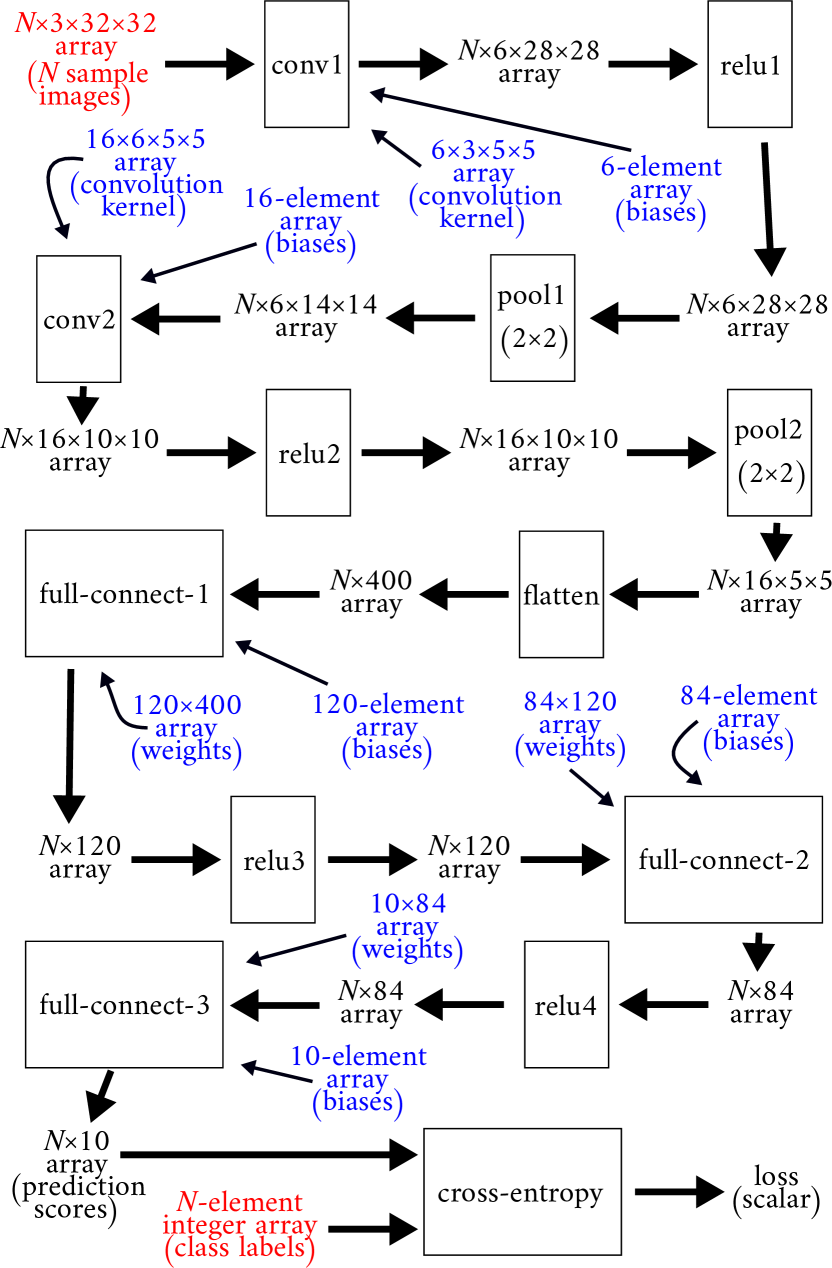
Figure 1: Structure of the CNN for classifying images. Steps of computation are framed, while their inputs and outputs are not. Data (parts of $\mathcal{D}$) are marked in red, while parameters (parts of $\mathcal{P}$) are marked in blue.

Now, we essentially need to express the boxed steps of computation in SQL, with data $\mathcal{D}$ in red and paramters $\mathcal{P}$ in blue given as SQL tables.

First and foremost, let us see what we can do with the convolution step conv1. In the SQL context, we provide the 4-dimensional ($N\times 3\times 32\times 32$) array of $N$ sample images as a relation samples with the following 5 columns.

image, channel, r, c	INTEGER
val	REAL

The names and types of the columns should be quite self-explanatory. The column image refers to indices in the first dimension of the original 4D array, taking the values from $0$ to $(N-1)$ (inclusive). Similarly, the column channel refers to which one of the three (RGB) channels (2nd dimension), while r and c refer to which row (3rd dimension) and which column (4th dimension) respectively. The column val stores the actual values in the array, obviously.

Similarly, the the $6\times 3\times 5\times 5$ array of the convolution kernel is presented as a relation conv1_weight with 5 columns.

out_channel, in_channel, r, c	INTEGER
weight	REAL

And the biases to the convolutional layer corresponds to a 2-column relation conv1_bias.

out_channel	INTEGER
bias	REAL

With the input relation ready, we can execute the computation of conv1 with CREATE TABLE commands. We do this in two steps. Firstly, we put the results of the convolution itself into conv1_unbiased.

⬇

CREATE TABLE conv1_unbiased AS

SELECT

image,

out_channel AS channel,

samples.r-conv1_weight.r AS r1,

samples.c-conv1_weight.c AS c1,

SUM(val * weight) AS val

FROM samples, conv1_weight

WHERE

channel = in_channel AND

r1 BETWEEN 0 AND 32-5 AND

c1 BETWEEN 0 AND 32-5

GROUP BY image,channel,r1,c1;

Then we apply the biases to get conv1_out.

⬇

CREATE TABLE conv1_out AS

SELECT

image, channel, r1 AS r, c1 AS c,

val + bias AS val

FROM conv1_unbiased,conv1_bias

WHERE channel = out_channel;

The ReLU layer relu1 is embarrassingly simple to compute.

⬇

CREATE TABLE relu1_out AS

SELECT

image, channel, r, c, MAX(0,val) AS val

FROM conv1_out

Executing max-pooling (pool1) is also straight-forward.

⬇

CREATE TABLE pool1_out AS

SELECT

image, channel, r/2 AS r, c/2 AS c,

MAX(val) AS val

FROM relu1_out GROUP BY image,channel, r, c;

Now the remaining computation steps up till flatten are almost identical to what we have listed except for table names and array dimensions. We skip them to assume having evaluated the output of pool2. flatten is almost as simple as ReLU.

⬇

CREATE TABLE flatten_out AS

SELECT

image, (channel * 5 + r)*5+c AS i, val

FROM pool2_out;

A fully-connected layer like fc1 is treated just like a convolution layer, only simpler. The weights and biases are put in the SQL context as fc1_weight with

out_dim, in_dim	INTEGER
weight	REAL

and fc1_bias with

out_dim	INTEGER
bias	REAL

.

Then we can compute fc1_out by applying weights and biases in two consecutive steps.

⬇

CREATE TABLE fc1_unbiased AS

SELECT

image, out_dim AS i,

SUM(val * weight) AS val

FROM flatten_out, fc1_weight

WHERE i = in_dim GROUP BY image, out_dim;

CREATE TABLE fc1_out AS

SELECT image, i, val + bias AS val

FROM fc1_unbiased,fc1_bias

WHERE i=out_dim;

At this point the computation in SQL up to the output of full-connect-3 should be clear. At this stage we could claim that we have specified the neural network per se. It is enough for executing inference. However for training, we still have to show how to compute cross-entropy.

Cross-entropy loss for one sample of computed label weights $\mathbf{x}$ whose correct label is $l$ is given by

$$\text{loss}(\mathbf{x},l)=-x_{l}+\log\limits(\sum_{j}\text{exp}(x_{j}))~{}.$$

And we choose to compute the loss over the $N$ samples as the mean over each sample. Assume the output of full-connect-3 to be fc3_out. First we compute the right side of “+” with

⬇

CREATE TABLE x_ent_losses_r AS

SELECT image, LOG(SUM(EXP(val))) AS r

FROM fc3_out GROUP BY image;

where LOG() and EXP() are obviously (element-wise) natural logarithm and exponentiation. The left hand side is just selecting one of 10 element, listed as follows list it for clarity.

⬇

CREATE TABLE x_ent_losses_l AS

SELECT fc3_out.image,-val AS l

FROM fc3_out, labels

WHERE

fc3_out.image = labels.image AND i = label;

Then we combine both sides to get loss for each image

⬇

CREATE TABLE x_ent_losses AS

SELECT image, l+r AS val

FROM

x_ent_losses_l NATURAL JOIN x_ent_losses_r;

and then finally the average loss

⬇

CREATE TABLE x_ent_loss AS

SELECT SUM(val)/COUNT(val)

FROM x_ent_losses;

as an 1-row table. Now we have finished specifying a deep learning model entirely in SQL.

4.2 Graph Convolutional Network

Now let us see a baisc Graphan Convolutional Network (GCN) setup in SQL. This GCN is adapted from a simplified version of that in [17], as a very neat tutorial provided by the same author [15]. We further remove the dropout to simplify things, which moderately increases the computation load and slightly increases overfitting while not changing major results.

The structure of the whole forward computation is as shown in Figure 2. This time we assume $N$ samples of $M$ features to be classified into $C$ classes, with one hidden layer of size $H$ in-between. This structure is actually much simpler than the previous example, the only really new things being the Graph Convolutional layers (gc1 and gc2) and the accompanying ($N\times N$) adjacency matrix $A$. So we will focus on them.

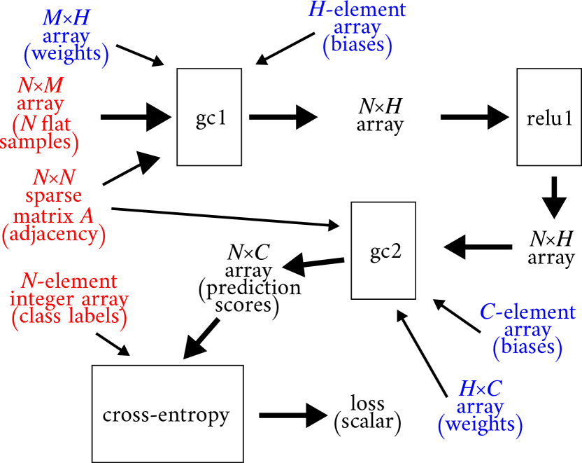
Figure 2: Structure of the simple examplar Graph Convolutional Network. Steps of computation are framed, while their inputs and outputs are not. Data (parts of $\mathcal{D}$) are marked in red, while parameters (parts of $\mathcal{P}$) are marked in blue.

From a computational point-of-view, what the Graph Convolutional layer can be considered as two consecutive matrix multiplications plus biasing, despite named “convolutional” layers. That is, the computation before biasing can be simply expressed as $AXW~{},$ where $X$ denotes the input of the layer and $W$ denotes the weights. Take gc1 for example, $X$ is an $N\times M$ matrix while while $W$ is $M\times H$. Then we can add the biases with

$$Y_{i,j}=(AXW)_{i,j}+B_{j}~{},$$

for all $i\in\{1..N\},j\in\{1..H\}$, $B$ being the biases of the layer gc1.

Now continuing with gc1, we assume the following tables in the SQL world.

⬇

samples(i INTEGER, j INTEGER, val REAL);

gc1_w (i INTEGER, j INTEGER, weight REAL);

gc1_b (i INTEGER, bias REAL);

adj (i INTEGER, j INTEGER, val REAL);

Drawing from previous experience from fully-connected layers, We can easily reproduce the above forward computation in SQL with

⬇

CREATE TABLE gc1_mid AS

SELECT

samples.i AS i, gc1_w.j AS j,

SUM(val * weight) AS val

FROM samples, gc1_w

WHERE samples.j == gc1_w.i

GROUP BY samples.i, gc1_w.j;

for the intermediate matrix product $XW$, and subsequently

⬇

CREATE TABLE gc1_out AS

SELECT

adj.i AS i, gc1_mid.j AS j,

SUM(adj.val * gc1_mid.val) + bias AS val

FROM adj, gc1_mid, gc1_b

WHERE

adj.j == gc1_mid.i AND gc1_mid.j == gc1_b.i

GROUP BY adj.i, gc1_mid.j;

for the whole biased output.

The symmetric adjacency matrix $A$ has zeroes for pairs of vertices without an edge in-between and non-zeroes for those connected by an edge. Furthermore, the adjacency matrix is row-normalized from a typical adjacency matrix of 0’s and 1’s. That is, each row sums to either 1 if there are any edges on the vertex or 0 if the vertex is complete isolated. And so does each column because of symmetry.

The adjacency matrix here is usually a sparse matrix. Or to put it another way, the sparsity is essential to its practical effectiveness, which in turn was probably an important precondition to its current popularity. Yet in the SQL world we do not treat sparsity as something special. Actually we take sparsity for granted. While how to create an implementation running as fast as array-based deep-learning frameworks is no easy task, we already have battle-hardened semantics and standards in the database world.

5 Discussion

The notion that databases provides the data for dedicated machine learning components to work on has been seldom questioned when unifiying the two fields. But we may as well go to the extent that we build machine learning programs in terms of databases.

In general, we could consider databases as the most feature-rich deep learning framework in the future. We look at databases and we know what can be added to deep learning.

One often overlooked fact is that datasets are processed as arrays, implying an order while they are not supposed to. Relational algebra and subsequently SQL take care of this automatically.

The biggest challenge for implementation would be to port automatic differentation to relational algebra. However it could also be implemented over yet another layer of flat array framework with automatic differentiation, treated as some kind of linear memory to sidestep automatic differentiation from the ground up.

Databases have been dealing with sparse data to begin with. While directly run deep learning in database engine may not be competitive as random access too much to be fast at batch processing, we can certainly continue to bring experience in database to machine learning for a very long time to come. Perhaps when new deep learning models are proposed, the machine learning researchers will find the database community waiting for them.

References

- [1] M. Abadi, A. Agarwal, P. Barham, E. Brevdo, Z. Chen, C. Citro, G. S. Corrado, A. Davis, J. Dean, M. Devin, S. Ghemawat, I. Goodfellow, A. Harp, G. Irving, M. Isard, Y. Jia, R. Jozefowicz, L. Kaiser, M. Kudlur, J. Levenberg, D. Mané, R. Monga, S. Moore, D. Murray, C. Olah, M. Schuster, J. Shlens, B. Steiner, I. Sutskever, K. Talwar, P. Tucker, V. Vanhoucke, V. Vasudevan, F. Viégas, O. Vinyals, P. Warden, M. Wattenberg, M. Wicke, Y. Yu, and X. Zheng. TensorFlow: Large-scale machine learning on heterogeneous systems, 2015. Software available from tensorflow.org.
- [2] M. Boehm, I. Antonov, M. Dokter, R. Ginthoer, K. Innerebner, F. Klezin, S. Lindstaedt, A. Phani, and B. Rath. Systemds: A declarative machine learning system for the end-to-end data science lifecycle. 09 2019.
- [3] M. Boehm, M. W. Dusenberry, D. Eriksson, A. V. Evfimievski, F. M. Manshadi, N. Pansare, B. Reinwald, F. R. Reiss, P. Sen, A. C. Surve, et al. Systemml: Declarative machine learning on spark. Proceedings of the VLDB Endowment, 9(13):1425–1436, 2016.
- [4] J. V. D’silva, F. De Moor, and B. Kemme. Aida: abstraction for advanced in-database analytics. Proceedings of the VLDB Endowment, 11(11):1400–1413, 2018.
- [5] J. V. D’silva, F. De Moor, and B. Kemme. Making an RDBMS data scientist friendly: Advanced in-database interactive analytics with visualization support. PVLDB, 12(12):1930–1933, 2019.
- [6] L. Du. How much deep learning does neural style transfer really need? an ablation study. In The IEEE Winter Conference on Applications of Computer Vision (WACV), March 2020.
- [7] Y. Feng, H. You, Z. Zhang, R. Ji, and Y. Gao. Hypergraph neural networks. In Proceedings of the AAAI Conference on Artificial Intelligence, volume 33, pages 3558–3565, 2019.
- [8] L. A. Gatys, A. S. Ecker, and M. Bethge. Image style transfer using convolutional neural networks. In Proceedings of the IEEE Conference on Computer Vision and Pattern Recognition, Jun 2016.
- [9] I. J. Goodfellow, J. Shlens, and C. Szegedy. Explaining and harnessing adversarial examples. arXiv preprint arXiv:1412.6572, 2014.
- [10] J. M. Hellerstein, C. Ré, F. Schoppmann, D. Z. Wang, E. Fratkin, A. Gorajek, K. S. Ng, C. Welton, X. Feng, K. Li, et al. The madlib analytics library. Proceedings of the VLDB Endowment, 5(12), 2012.
- [11] J. Jiang, Y. Wei, Y. Feng, J. Cao, and Y. Gao. Dynamic hypergraph neural networks. In Proceedings of the 28th International Joint Conference on Artificial Intelligence, pages 2635–2641. AAAI Press, 2019.
- [12] W. W. C. F. Y. Kathryn and R. Mazaitis. Tensorlog: Deep learning meets probabilistic databases. Journal of Artificial Intelligence Research, 1:1–15, 2018.
- [13] S. M. Kazemi and D. Poole. Relnn: A deep neural model for relational learning. In Thirty-Second AAAI Conference on Artificial Intelligence, 2018.
- [14] M. Kim. TensorDB and tensor-relational model (TRM) for efficient tensor-relational operations. Arizona State University, 2014.
- [15] T. N. Kipf. https://github.com/tkipf/pygcn.
- [16] T. N. Kipf and M. Welling. Semi-supervised classification with graph convolutional networks. 2016.
- [17] T. N. Kipf and M. Welling. Semi-supervised classification with graph convolutional networks. arXiv preprint arXiv:1609.02907, 2016.
- [18] X. Li, B. Cui, Y. Chen, W. Wu, and C. Zhang. Mlog: Towards declarative in-database machine learning. Proceedings of the VLDB Endowment, 10(12):1933–1936, 2017.
- [19] W. McKinney. Data structures for statistical computing in python. In S. van der Walt and J. Millman, editors, Proceedings of the 9th Python in Science Conference, pages 51 – 56, 2010.
- [20] S. S. Sandha, W. Cabrera, M. Al-Kateb, S. Nair, and M. Srivastava. In-database distributed machine learning: Demonstration using teradata sql engine. Proc. VLDB Endow., 12(12):1854–1857, Aug. 2019.
- [21] A. Santoro, R. Faulkner, D. Raposo, J. Rae, M. Chrzanowski, T. Weber, D. Wierstra, O. Vinyals, R. Pascanu, and T. Lillicrap. Relational recurrent neural networks. In Advances in neural information processing systems, pages 7299–7310, 2018.
- [22] A. Santoro, D. Raposo, D. G. Barrett, M. Malinowski, R. Pascanu, P. Battaglia, and T. Lillicrap. A simple neural network module for relational reasoning. In I. Guyon, U. V. Luxburg, S. Bengio, H. Wallach, R. Fergus, S. Vishwanathan, and R. Garnett, editors, Advances in Neural Information Processing Systems 30, pages 4967–4976. Curran Associates, Inc., 2017.
- [23] F. Scarselli, M. Gori, A. C. Tsoi, M. Hagenbuchner, and G. Monfardini. The graph neural network model. IEEE Transactions on Neural Networks, 20(1):61–80, 2008.
- [24] M. Schlichtkrull, T. N. Kipf, P. Bloem, R. Van Den Berg, I. Titov, and M. Welling. Modeling relational data with graph convolutional networks. In European Semantic Web Conference, pages 593–607. Springer, 2018.
- [25] M. Schüle, F. Simonis, T. Heyenbrock, A. Kemper, S. Günnemann, and T. Neumann. In-database machine learning: Gradient descent and tensor algebra for main memory database systems. BTW 2019, 2019.
- [26] M. E. Schüle, M. Bungeroth, D. Vorona, A. Kemper, S. Günnemann, and T. Neumann. Ml2sql - compiling a declarative machine learning language to sql and python. In EDBT, 2019.
- [27] M. Schüle, M. Bungeroth, A. Kemper, S. Günnemann, and T. Neumann. Mlearn: A declarative machine learning language for database systems. pages 1–4, 06 2019.
- [28] G. Sourek, V. Aschenbrenner, F. Zelezny, S. Schockaert, and O. Kuzelka. Lifted relational neural networks: Efficient learning of latent relational structures. Journal of Artificial Intelligence Research, 62:69–100, 2018.
- [29] M. Stonebraker, P. Brown, J. Becla, and D. Zhang. Scidb: A database management system for applications with complex analytics. Computing in Science and Engg., 15(3):54–62, May 2013.
- [30] M. Stonebraker, P. Brown, A. Poliakov, and S. Raman. The architecture of scidb. In Proceedings of the 23rd International Conference on Scientific and Statistical Database Management, SSDBM’11, page 1–16, Berlin, Heidelberg, 2011. Springer-Verlag.
- [31] W. Uwents and H. Blockeel. Classifying relational data with neural networks. In S. Kramer and B. Pfahringer, editors, Inductive Logic Programming, pages 384–396, Berlin, Heidelberg, 2005. Springer Berlin Heidelberg.
- [32] W. Uwents, G. Monfardini, H. Blockeel, M. Gori, and F. Scarselli. Neural networks for relational learning: an experimental comparison. Machine Learning, 82:315–349, 03 2011.
- [33] W. Wang, M. Zhang, G. Chen, H. Jagadish, B. C. Ooi, and K.-L. Tan. Database meets deep learning: Challenges and opportunities. ACM SIGMOD Record, 45(2):17–22, 2016.
- [34] N. Yadati, M. Nimishakavi, P. Yadav, V. Nitin, A. Louis, and P. Talukdar. Hypergcn: A new method for training graph convolutional networks on hypergraphs. In Advances in Neural Information Processing Systems, pages 1509–1520, 2019.
- [35] V. Zambaldi, D. Raposo, A. Santoro, V. Bapst, Y. Li, I. Babuschkin, K. Tuyls, D. Reichert, T. Lillicrap, E. Lockhart, M. Shanahan, V. Langston, R. Pascanu, M. Botvinick, O. Vinyals, and P. Battaglia. Deep reinforcement learning with relational inductive biases. In International Conference on Learning Representations, 2019.