Dynamically screened vertex correction to $GW$

Abstract

Diagrammatic perturbation theory is a powerful tool for the investigation of interacting many-body systems, the self-energy operator $\Sigma$ encoding all the variety of scattering processes. In the simplest scenario of correlated electrons described by the $GW$ approximation for the electron self-energy, a particle transfers a part of its energy to neutral excitations. Higher-order (in screened Coulomb interaction $W$) self-energy diagrams lead to improved electron spectral functions (SF) by taking more complicated scattering channels into account and by adding corrections to lower order self-energy terms. However, they also may lead to unphysical negative spectral function. The resolution of this difficulty has been demonstrated in our previous works. The main idea is to represent the self-energy operator in a Fermi Golden rule form which leads to the manifestly positive definite SF and allows for a very efficient numerical algorithm. So far, the method has only been applied to 3D electron gas, which is a paradigmatic system, but a rather simple one. Here, we systematically extend the method to 2D including realistic systems such as mono and bilayer graphene. We focus on one of the most important vertex function effects involving the exchange of two particles in the final state. We demonstrate that it should be evaluated with the proper screening and discuss its influence on the quasiparticle properties.

I Introduction

Numerous correlated electron calculations follow a canonical scheme formulated by Hedin Hedin (1965) in terms of dressed propagators. It is now well established that the lowest-order self-energy (SE) term, the so-called $GW$ approximation is the major source of electronic correlations. Much less is known about the next perturbative orders: there is no single standard way of evaluating them despite the fact that there is a single second-order self-energy diagram (Fig. 1). There are multiple reasons for this. On one side, at the advent of many-body perturbation theory (MBPT) the computational power was insufficient to perform these demanding calculations, and one was forced to use some drastic simplifications. On the other side, there are several conceptual problems with the organization of many-body perturbation theory (MBPT) for interacting electrons. For instance, it is known that higher-order diagrammatic approximations for the electron self-energy in terms of the screened Coulomb interaction $W$ leads to poles in the “wrong” part of the complex plane giving rise to negative spectral densities. This observation has been made long time ago by Minnhagen Minnhagen (1974, 1975), and in our recent works we provided a general solution to this problem Stefanucci et al. (2014); Uimonen et al. (2015) yielding positive definite (PSD) spectral functions. The idea was to write the self-energy in the Fermi Golden rule form well known from the scattering theory.

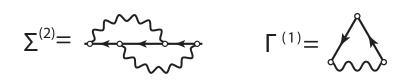
Figure 1: A single second-order self-energy diagram and the associated first-order vertex function in terms of the electron propagators (arrows) and the screened interactions (wavy lines).

One interesting conclusion of our theory is that the second-order SE describes three distinct scattering processes that take place in a many-body system Pavlyukh et al. (2016): (I) A correction to the first-order scattering, involving the same final states as in $GW$. This effect was numerically studied in Ref. Stefanucci et al. (2014), and has been shown Pavlyukh et al. (2016) to counteract the smearing out of spectral features in self-consistent calculations Holm and von Barth (1998). (II) Excitation of two plasmons ($pl$), or two particle-hole pairs ($p$-$h$), or a mixture of them in the final state. Especially the generation of two plasmons is a prominent effect spectroscopically manifested as a second satellite in the photoemission spectrum Riley et al. (2018). This effect can be obtained from the cumulant expansion Holm and Aryasetiawan (1997); Guzzo et al. (2014), which, however, only works at the band bottom $k=0$, or from the Langreth model Langreth (1970); Pavlyukh (2017). (III) A first-order scattering involving the exchange of the two final state particles. This latter scattering process is the focus of the present work.

Some manifestations of the mechanism (III) have already been studied, albeit without realizing its deep connection with the full $\Sigma^{(2)}$. First of all, for the two bare interaction lines we get the so-called second-order exchange, which has been shown to play an important role in correlated electronic calculations for molecular systems as an ingredient of the second-Born approximation (2BA) Balzer et al. (2010); Perfetto et al. (2015); Schüler and Pavlyukh (2018). Second, it yields a very important total energy correction for the homogeneous electron gas Ziesche (2007). Third, the mechanism with screening has been considered in the calculations of quasiparticle life-times. Reizer and Wilkins predicted that this diagram yields a 50% reduction of the scattering rate in 2D electron gas calling it “a nongolden-rule” contribution, whereas Qian and Vignale Qian and Vignale (2005) correctly pointed out that it is “still described by the Fermi golden rule, provided one recognizes that the initial and final states are Slater determinants”, and that the coefficient is different. Fourth, the mechanism is relevant for the scattering theory Almbladh (2006). With bare Coulomb interactions it represents the so-called double photoemission (DPE) process, and if the interaction is screened — the plasmon assisted DPE Pavlyukh et al. (2015); Schüler et al. (2016). Finally, the considered mechanism has some features in common with the second-order screened exchange (SOSEX) approximation Grüneis et al. (2009); Ren et al. (2015). However, there are also important differences in the constituent screened Coulomb interaction that will be explained below.

As can be seen from this list, the mechanism is an indispensable part of various physical processes. However, it has not been sufficiently emphasized that all of them can be derived from a single $\Sigma^{(2)}$ diagram. Moreover, there are no systematic studies of its impact on the quasiparticle properties other than the life-times. These gaps are filled in here. Our theoretical derivations are illustrated by calculations for four prominent systems: the homogeneous electron gas in two and three dimensions and the mono- and bilayer graphene. While the former two are very well studied model systems Lundqvist (1968); Santoro and Giuliani (1989), graphene is a real material, and while the $GW$ calculations for it exists Hwang and Das Sarma (2008a); Polini et al. (2008); Sensarma et al. (2011), MBPT has mostly been used in the renormalization group sense Kotov et al. (2012). Little is known about the frequency dependence of higher-order self-energies.

Our approach consists of analytical and numerical parts. For the quasiparticle ($qp$) electron Green’s function ($G_{0}$) and the screened interaction ($W_{0}$) in the random phase approximation (RPA), the frequency integration of a selected set of the electron self-energy ($\Sigma[G_{0},W_{0}]$) diagrams is performed in closed form using our symbolic algorithm implemented in mathematica computer algebra system. The remaining momentum integrals are performed numerically in line with our previous studies using the Monte Carlo approach Pavlyukh et al. (2013); Stefanucci et al. (2014); Uimonen et al. (2015); Pavlyukh et al. (2016) showing excellent accuracy and scalability. First, we evaluate the scattering rate function

$$\Gamma(k,\omega) =i\left[\Sigma_{c}^{>}(k,\omega)-\Sigma_{c}^{<}(k,\omega)\right],$$ (1)

and then the retarded self-energy via the Hilbert transform (Appendix A)

$$\Sigma^{\text{R}}(k,\omega) =\Sigma_{x}(k)+\int\frac{d\omega^{\prime}}{2\pi}\frac{\Gamma\left(k,\omega^{\prime}\right)}{\omega-\omega^{\prime}+i\eta},$$ (2)

where $\Sigma_{x}(k)$ is the frequency-independent exchange self-energy, and the meaning of greater $>$ and lesser $<$ components of the correlated self-energy $\Sigma_{c}$ is explained in the next section. Via the Dyson equation (Appendix E), the retarded self-energy determines correlated electronic structure.

Our work is structured as follows: we review our PSD approach in Sec. II and illustrate it with a concrete set of diagrams in Sec. III. Next we discuss the building blocks of our diagrammatic perturbation theory and provide reference $G_{0}W_{0}$ calculations for the four systems in Sec. IV. Efficient evaluation of screening is an important ingredient. In Sec. V we present our main numerical results: spectral features in $\Sigma^{(2)}$, cancellations between the first and the second order self-energies in the asymptotic regime, quasiparticle properties such as quasiparticle peak strengths, effective masses, velocities, and life-times. We finally present our conclusions and outlooks in Sec. VI.

II Summary of the PSD approach

Besides numerical difficulties, the major reason on why the MBPT calculations for the electron gas have not been systematically performed at higher orders is the fact that resulting expansions do not generate positive definite (PSD) spectral functions at all frequency and momentum values. How to deal with this obstacle is discussed in details in Refs. Stefanucci et al. (2014); Uimonen et al. (2015).

Even though this is an equilibrium problem, our method can most easily be formulated by using the nonequilibrium Green’s function (NEGF) formalism Stefanucci and van Leeuwen (2013). The main distinction is that field operators ($\hat{\psi}(\mathbf{x},z)$ and $\hat{\psi}^{\dagger}(\mathbf{x},z)$ for electrons) evolve on the time-loop contour $z\in\mathcal{C}$ with one forward chronologically ordered ($\mathcal{C}-$) branch and one ($\mathcal{C}^{+}$) branch with anti-chronological time-ordering, $\mathcal{C}=\mathcal{C}^{-}\cup\mathcal{C}^{+}$. Correspondingly, the two times Green’s functions generalize to $G(\mathbf{x}_{1}z_{1},\mathbf{x}_{2}z_{2})$ or $G^{\alpha\beta}(\mathbf{x}_{1}t_{1},\mathbf{x}_{2}t_{2})$, where $t_{1}$ and $t_{2}$ are the projections of $z_{1,2}$ on the real time-axis, and $\alpha,\beta=+/-$ indicate to which branches of the Keldysh contour they belong. In the following, we will explicitly deal with the lesser self-energy $\Sigma^{<}\equiv\Sigma^{-+}$, which describes scattering processes on the subspace of states below the Fermi level, i. e., holes. The greater component ($\Sigma^{>}\equiv\Sigma^{+-}$) can be treated analogously.

Figure 2: Half-diagrams for $D(2)$, the constituent of the $\Sigma^{<}(1,2)$ SE. All vertices are on the $\mathcal{C}^{+}$ branch. Wavy lines stand for the screened interaction $W$.

The PSD property concerns the fact that the rate operator (1) must be positive for all momentum $k$ and frequency $\omega$ values. $\Sigma_{c}$ with this property is diagrammatically constructed starting from any given set of diagrams as follows.

On the first step pluses and minuses are assigned to the diagram vertices in all possible combinations. They carry information about the contour times. The resulting decorated diagrams are called partitions. Since we have shown that at zero temperature no isolated $+$ or $-$ islands can exist Stefanucci et al. (2014), the “cutting” procedure splits the diagrams for $\Sigma_{c}^{<}$ into halves that have their vertices exclusively either on the ($-$) or on the ($+$) branch (viz. Fig. 2). They are the building blocks of the PSD construction. Subsequently, the half-diagrams are combined in such a way that a sum of complete squares is formed. This guarantees the positivity of the resulting set of diagrams. On the language of scattering theory, the half-diagrams have a meaning of the $S$-matrices describing various particle or hole scattering processes in a many-body system. The resulting PSD self-energies have then the Fermi Golden rule form, which always leads to positive scattering rates. Topologically distinct $S$-matrices will be denoted as $D$ diagrams. Diagrams that can be obtained by the cutting procedure applied to $\Sigma_{c}$ of the first- and second-order in $W_{0}$ are depicted in Fig. 2.

They are interpreted according to the standard diagrammatic rules. Consider for instance the half-diagrams with all the time-arguments on the $+$ branch (such as depicted in Fig. 2). In addition to the initial one-hole ($1h$) state (with the coordinate $2$, where the composite position-spin and time variables are abbreviated as $i\equiv(\mathbf{x}_{i},t_{i})$), the final state is denoted by the two strings of numbers $\underline{\mathscr{p}}=(\mathscr{p}_{1},\ldots\mathscr{p}_{N},\mathscr{p}_{N+1})$ and $\underline{\mathscr{q}}=(\mathscr{q}_{1},\ldots\mathscr{q}_{N})$ that specify composite coordinates of the outgoing $N+1$ holes and $N$ particles, respectively. We further associate a single time-argument $\tau$ with $(\underline{\mathscr{p}},\underline{\mathscr{q}})$. $\tau$ is the latest time on the forward and the earliest time on the backward contour branches. With these notations, $D^{(a)}$ reads

$$D^{(a)}_{\mathscr{p}_{1},\mathscr{p}_{2},\mathscr{q}_{1}}(2) =-(-1)^{1}\int\!\mathrm{d}(4)\,W_{0}^{++}(4,2)g^{<}(\mathscr{p}_{2}\tau,2)$$

$$\quad\times g^{<}(\mathscr{p}_{1}\tau,4)g^{>}(4,\mathscr{q}_{1}\tau),$$ (3a)

and its complex conjugate is given by

$$\big{[}D^{(a)}_{\mathscr{p}_{1},\mathscr{p}_{2},\mathscr{q}_{1}}(1)\big{]}^{*} =+\int\!\mathrm{d}(3)\,W_{0}^{--}(1,3)g^{<}(1,\mathscr{p}_{2}\tau)$$

$$\quad\times g^{<}(3,\mathscr{p}_{1}\tau)g^{>}(\mathscr{q}_{1}\tau,3),$$ (3b)

where the extra minus sign $(-1)^{1}$ in Eq. (3a) is due to the fact that for each time-integration associated with a vertex on $\mathcal{C}^{+}$

$$\int_{\mathcal{C}^{+}}\mathrm{d}z_{i}\ldots =-\int_{-\infty}^{\infty}\mathrm{d}t_{i}\ldots.$$ (4)

Eqs. (3) are expressed in terms of the bare electron propagators $g(\mathbf{x}_{1},t_{1};\mathbf{x}_{2},t_{2})$ and the RPA screened interaction

$$W_{0}(1,2) =\int\mathrm{d}(3)v(1,3)\,\varepsilon_{0}^{-1}(3,2),$$ (5)

where $\varepsilon_{0}$ is the RPA dielectric function defined in terms of the polarization bubble $\mathcal{P}_{0}$ and the bare Coulomb interaction $v$,

$$\varepsilon_{0}(1,2) =\delta(1,2)-\int\mathrm{d}(3)\,v(1,3)\mathcal{P}_{0}(3,2),$$ (6)

$$\mathcal{P}_{0}(1,2) =-ig(1,2)g(2,1).$$ (7)

In Eqs. (3), $W_{0}^{--}\equiv W_{0}^{\text{T}}$ and $W_{0}^{++}\equiv W_{0}^{\overline{\text{T}}}$ stand for the time-ordered and anti-time-ordered interactions, respectively. We refer to App. B for the detailed definitions and Sec. IV for explicit forms of the dielectric function for the four studied systems. $D^{(b)}$ and $D^{(c)}$ are defined analogously. Our next goal is to describe self-energies that are obtained by “gluing” the $D$-diagrams. This is complementary to our earlier works Stefanucci et al. (2014); Uimonen et al. (2015), where the half-diagrams were derived by the “cutting” rules.

III Self-energy approximations: physical meaning of diagrams

It is straightforward to see that by ‘gluing” three half-diagrams $D^{\text{(i)}}(2)$ ($\text{i}=a,b,c$, Fig. 2) with their complex conjugates $[D^{\text{(i)}}(1)]^{*}$ with or without permutations of internal coordinates, one obtains the four classes shown in Fig. 3(a). They are grouped into three terms covering three distinct physical mechanisms

$$\Sigma_{\text{PSD}}^{<}(1,2)=\Sigma^{<}_{aa}(1,2)+[\Sigma^{<}_{cc}(1,2)+\Sigma^{<}_{c\bar{c}}(1,2)]+\Sigma^{<}_{a\bar{a}}(1,2),$$ (8)

In Ref. Stefanucci et al. (2014) we have also shown that this is the minimal set of diagrams covering all the first- and second-order self-energies and possessing the PSD property. Let us discuss the involved physical mechanisms and derive the working formulas.

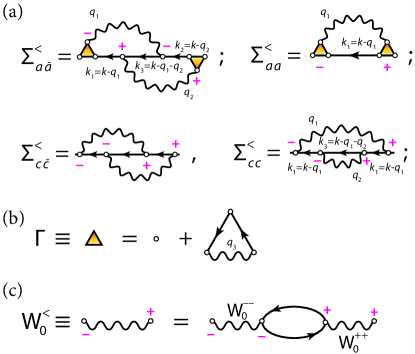
Figure 3: (a) The contributions to $\Sigma_{\text{PSD}}^{<}$ given by Eq. (8) and arising from the first- and second-order (in screened interaction) self-energy by virtue of the PSD procedure (Sec. II). Three subsets of these diagrams that also fulfill the PSD property are given by Eqs. (106). (b) First order vertex function $\mathsf{\Gamma}$. (c) Random phase approximation for the lesser component of the screened Coulomb interaction.

III.1 $\Sigma_{aa}^{<}$

$\Sigma_{aa}^{<}$ without vertex corrections is nothing else as the first-order ($GW$) self-energy. It results from the gluing the simplest half-diagram $D^{(a)}$ [Fig. 2(a)] with itself without permuting the two hole lines ($\mathscr{p}_{1}$ and $\mathscr{p}_{2}$):

$$\Sigma_{GW}^{<}(1,2) =i\sum_{\mathscr{p}_{1},\mathscr{p}_{2},\mathscr{q}_{1}}\big{[}D_{\mathscr{p}_{1},\mathscr{p}_{2},\mathscr{q}_{1}}^{(a)}(1)\big{]}^{*}D^{(a)}_{\mathscr{p}_{1},\mathscr{p}_{2},\mathscr{q}_{1}}(2)$$

$$=ig^{<}(1,2)W_{0}^{<}(1,2).$$ (9)

In order to establish the second equality, we use the explicit form of the half-diagrams (3), recall that $ig^{<}(1,2)=\sum_{\mathscr{p}_{2}}g^{<}(1,\mathscr{p}_{2}\tau)g^{<}(\mathscr{p}_{2}\tau,2)$, $ig^{<}(3,4)=\sum_{\mathscr{p}_{1}}g^{<}(3,\mathscr{p}_{1}\tau)g^{<}(\mathscr{p}_{1}\tau,4)$, and $-ig^{>}(4,3)=\sum_{\mathscr{q}_{1}}g^{>}(4,\mathscr{q}_{1}\tau)g^{>}(\mathscr{q}_{1}\tau,3)$, and that the lesser screened interaction can be written in the form

$$W_{0}^{<}(1,2) =-\!\iint\!\!\mathrm{d}(3,4)\,W_{0}^{--}(1,3)\mathcal{P}^{<}_{0}(3,4)W_{0}^{++}(4,2),$$

with $\mathcal{P}^{<}_{0}(3,4)=-ig^{<}(3,4)g^{>}(4,3)$ as shown in Fig. 3(c).

Now we use the diagrams in momentum and frequency representation as indicated in Fig. 3, namely

$$\bm{\mathit{k}}_{1} =\bm{\mathit{k}}-\bm{\mathit{q}}_{1}, \bm{\mathit{k}}_{2} =\bm{\mathit{k}}-\bm{\mathit{q}}_{2}, \bm{\mathit{k}}_{3} =\bm{\mathit{k}}-\bm{\mathit{q}}_{1}-\bm{\mathit{q}}_{2},$$ (10)

in order to derive a standard result for the $GW$ self-energy:

$$\Sigma_{GW}^{<}(k,\omega) =i\int\mathrm{d}\Omega_{1}\int\frac{\mathrm{d}\nu_{1}}{2\pi}\,g^{<}(k_{1},\omega-\nu_{1})$$

$$\qquad\times W_{0}^{<}(q_{1},\nu_{1}),$$ (11)

where $\int\mathrm{d}\Omega_{1}\equiv\int\frac{\mathrm{d}^{d}\bm{\mathit{q}}_{1}}{(2\pi)^{d}}$ denotes an integral over a $d$-dimensional momentum space, $\omega$ is the external frequency and $\bm{\mathit{k}}$ is the momentum. For graphene systems, the integration additionally contains a sum over the bands and a respective scattering matrix element. We will generally use $\omega_{i}$ and $\bm{\mathit{k}}_{i}$ for the energy and momentum of fermionic lines, and $\nu_{i}$ and $\bm{\mathit{q}}_{i}$ for the interaction lines.

Introducing the spectral function of the screened interaction $C(q,\nu)$ and using explicit formulas for the bare propagators in Appendix B and in particular

$$g^{<}(k,\omega) =2\pi in_{\text{F}}(k)\operatorname{\delta}(\omega-\epsilon(k)),$$ (12)

$$W_{0}^{<}(q,\nu) =-2\pi i\operatorname{\theta}(-\nu)C(q,-\nu),$$ (13)

where $n_{\text{F}}(k)\equiv n_{\text{F}}(\epsilon(k))$ is the fermion occupation number, we obtain

$$\Sigma_{GW}^{<}(k,\omega) =2i\pi\int\mathrm{d}\Omega_{1}\int_{0}^{\infty}\mathrm{d}\nu_{1}\,n_{\text{F}}(k_{1})C(q_{1},\nu_{1})$$

$$\qquad\times\operatorname{\delta}(\omega+\nu_{1}-\epsilon_{1}),$$ (14)

with $\epsilon_{i}\equiv\epsilon(\bm{\mathit{k}}_{i})$. As long as the spectral function of neutral excitations is positive, $C(q,\nu)>0$ (which is indeed the case because we use RPA for $W_{0}$ here Uimonen et al. (2015)), the rate operator [$-i\Sigma_{GW}^{<}(k,\omega)$] is positive too, as evident from Eq. (14), and the nature of the final scattering state is revealed: it consists of a hole with energy $\epsilon_{1}-\nu_{1}$ and a neutral excitation such as $p$-$h$ pair or a plasmon with momentum $q_{1}$ and energy $\nu_{1}$.

Eq. (9) can be extended by adding internal interaction lines to $D^{(a)}$ and maintaining the external indices and the way how the constituent half-diagrams are glued. The $b$-half-diagram depicted in Fig. 2(b) represents the simplest possibility

$$\Sigma_{aa}^{<}(1,2) =i\sum_{\mathscr{p}_{1},\mathscr{p}_{2},\mathscr{q}_{1}}\big{[}D^{(a)}+D^{(b)}\big{]}_{\mathscr{p}_{1},\mathscr{p}_{2},\mathscr{q}_{1}}^{*}(1)$$

$$\quad\quad\quad\times\big{[}D^{(a)}+D^{(b)}\big{]}_{\mathscr{p}_{1},\mathscr{p}_{2},\mathscr{q}_{1}}(2).$$ (15)

$D^{(b)}$ has one extra interaction line and therefore by gluing it with $D^{(a)}$ leads to two equivalent terms of the second order in $W_{0}$, and by gluing $D^{(b)}$ with itself to a term of third order. They can conveniently be represented by introducing the vertex function $\mathsf{\Gamma}$ depicted as yellow triangle in Fig. 3 (a,b) and familiar from the Hedin’s functional equations Hedin (1965); Strinati (1988). If one starts from higher-order diagrams, the diagrammatic expansion of $\mathsf{\Gamma}$ becomes more complicated and starts to differ from the standard vertex function. As in the case of $\Sigma_{GW}$, the electronic and the interaction lines connecting the $+$ and $-$ islands are given by the lesser propagators $g^{<}(k_{1},\omega-\nu_{1})$ and $W^{<}(q_{1},\nu_{1})$. In view of the energy conservation, only these two propagators depend on $\nu_{1}$, and the frequency integration can likewise be performed. It is clear that the same functional form proportional to $n_{\text{F}}(\omega+\nu_{1})\delta(\omega-\epsilon_{1}+\nu_{1})$ is obtained. Therefore, we conclude that $D^{(b)}$ renormalizes the $GW$ expression, but does not lead to new spectral features. Eq. (15) is a complete square, therefore $\Sigma_{aa}^{<}(1,2)$ is PSD. It was numerically evaluated in our earlier work Stefanucci et al. (2014).

III.2 $\Sigma_{c\bar{c}}^{<}$ and $\Sigma_{cc}^{<}$

The same analysis can be applied to other diagrams. $\Sigma_{c\bar{c}}^{<}$ and $\Sigma_{cc}^{<}$ feature the $--++$ partition (in this notation the vertices are traversed along the fermionic lines from 1 to 2 in the order opposite to arrows) and contain two diagrams from gluing the half-diagrams of the $c$-type [Fig. 2(c)] $[D^{(c)}(1)]^{*}$ and $D^{(c)}(2)$ with and without permutation of the dangling fermionic lines, respectively:

$$\Sigma_{cc}^{<}(1,2)+\Sigma_{c\bar{c}}^{<}(1,2)=i\sum_{\underline{\mathscr{p}},\underline{\mathscr{q}}}\big{[}D^{(c)}_{\mathscr{p}_{1},\mathscr{p}_{2},\mathscr{p}_{3},\mathscr{q}_{1},\mathscr{q}_{2}}(1)\\ +D^{(c)}_{\mathscr{p}_{2},\mathscr{p}_{1},\mathscr{p}_{3},\mathscr{q}_{2},\mathscr{q}_{1}}(1)\big{]}^{*}D^{(c)}_{\mathscr{p}_{1},\mathscr{p}_{2},\mathscr{p}_{3},\mathscr{q}_{1},\mathscr{q}_{2}}(2).$$ (16)

Explicit derivation of this expression in momentum-energy representation goes beyond the scope of this work. However, some physical insight can be gained by using the plasmon-pole approximation $C(q,\nu)=C(q)\delta(\nu-\Omega(q))$ for the screened interaction (13). As can be seen from the diagrammatic representation (Fig. 3) of self-energy (16), there are 3 lesser propagators connecting the $+$ and $-$ islands, which in the energy-momentum representation read: $g^{<}(k_{3},\omega-\nu_{1}-\nu_{2})W^{<}(q_{1},\nu_{1})W^{<}(q_{2},\nu_{2})$. In view of the energy conservation these are the only propagators that depend on the frequencies $\nu_{1,2}$. Therefore, the integrals can be explicitly performed. A scattering process accompanied by the generation of two plasmons can be inferred from the resulting frequency dependence proportional to $n_{\text{F}}(\omega+\Omega(q_{1})+\Omega(q_{2}))\delta(\omega-\epsilon_{3}+\Omega(q_{1})+\Omega(q_{2}))$, and is PSD per construction.

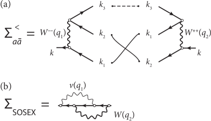
Figure 4: (a) Gluing two $D^{(a)}$ half-diagrams with one permutation of the two hole lines with momenta $\bm{\mathit{k}}_{1}=\bm{\mathit{k}}-\bm{\mathit{q}}_{1}$ and $\bm{\mathit{k}}_{2}=\bm{\mathit{k}}-\bm{\mathit{q}}_{2}$ and a single hole line $\bm{\mathit{k}}_{3}=\bm{\mathit{k}}-\bm{\mathit{q}}_{1}-\bm{\mathit{q}}_{2}$ (dashed) yields $\Sigma_{a\bar{a}}^{<}(k,\omega)$. The unpermuted configuration is not included, therefore the diagram may lead to a negative electron spectral function. Wavy lines denote screened Coulomb interactions. (b) $\Sigma_{\text{SOSEX}}^{<}$ contains different interaction lines and is thus distinct from $\Sigma_{a\bar{a}}^{<}$.

III.3 $\Sigma_{a\bar{a}}^{<}$

Finally we consider a rather complicated $\Sigma_{a\bar{a}}^{<}$ resulting from the $-+-+$ partition, Fig. 3 (a):

$$\Sigma_{a\bar{a}}^{<}(1,2) =-i\sum_{\mathscr{p}_{1},\mathscr{p}_{2},\mathscr{q}_{1}}\!\big{[}D^{(a)}+D^{(b)}\big{]}_{\mathscr{p}_{2},\mathscr{p}_{1},\mathscr{q}_{1}}^{*}(1)$$

$$\qquad\qquad\times\big{[}D^{(a)}+D^{(b)}\big{]}_{\mathscr{p}_{1},\mathscr{p}_{2},\mathscr{q}_{1}}(2).$$ (17)

It has a form very similar to Eq. (15), except the hole indices $\mathscr{p}_{1}$ and $\mathscr{p}_{2}$ are permuted (Fig. 4) leading to the change of sign. The sign of a permutation can be conveniently determined from the number of crossing of fermionic lines connecting the half-diagrams van Leeuwen and Stefanucci (2012). Neglecting the $D^{(b)}$ diagrams, which only produces a correction to the scattering of a hole state into a 2-holes-1-particle state, and using the explicit form for $D^{(a)}$, Eqs. (3), the self-energy in coordinate representation reads

$$\Sigma_{a\bar{a}}^{<}(1,2)=-\iint\mathrm{d}(3,4) \,W^{--}(1,3)g^{<}(1,4)g^{>}(4,3)$$

$$\quad\times g^{<}(3,2)W^{++}(4,2).$$ (18)

Thus, there are 2 lesser and 1 greater propagators connecting the $+$ and the $-$ islands. In the momentum-frequency representation they are $g^{>}(k_{3},\omega-\nu_{1}-\nu_{2})g^{<}(k_{1},\omega-\nu_{1})g^{<}(k_{2},\omega-\nu_{2})$. They contain $\delta$-functions, therefore, the integrals over the internal frequencies $\nu_{1,2}$ are simple. Collecting screened interaction dependent on these frequencies, $W^{--}(q_{1},\nu_{1})W^{++}(q_{2},\nu_{2})$, and using the explicit form

$$g^{>}(k,\omega) =-2\pi i\bar{n}_{\text{F}}(k)\delta(\omega-\epsilon(k)),$$ (19)

with $\bar{n}_{\text{F}}(k)=1-n_{\text{F}}(k)$, we can write the self-energy explicitly

$$\Sigma_{a\bar{a}}^{<}(k,\omega) =2i\pi\!\iint\!\mathrm{d}(\Omega_{1,2})\,n_{\text{F}}(\epsilon_{1})n_{\text{F}}(\epsilon_{2})\bar{n}_{\text{F}}(\epsilon_{3})$$

$$\qquad\times W^{--}(q_{1},\omega-\epsilon_{1})W^{++}(q_{2},\omega-\epsilon_{2})$$

$$\qquad\times\delta(\omega-\epsilon_{1}-\epsilon_{2}+\epsilon_{3})$$ (20)

$$=-2i\pi\!\iint\!\mathrm{d}(\Omega_{1,2})\,n_{\text{F}}(\epsilon_{1})n_{\text{F}}(\epsilon_{2})\bar{n}_{\text{F}}(\epsilon_{3})$$

$$\qquad\times\operatorname{Re}\left[W^{\text{T}}(q_{1},\omega-\epsilon_{1})\left(W^{\text{T}}(q_{2},\omega-\epsilon_{2})\right)^{*}\right]$$

$$\qquad\times\delta(\omega-\epsilon_{1}-\epsilon_{2}+\epsilon_{3}).$$ (21)

Because of the permutation of $\mathscr{p}_{1}$ and $\mathscr{p}_{2}$ indices, Eq. (17) forms a complete square only in combination with the unpermuted configuration, Eq. (15), and $-i\Sigma_{a\bar{a}}^{<}$ is not PSD on its own. At least for bare interactions, this can immediately be seen from the equation above. In this case the second-order exchange self-energy $\Sigma_{2x}$ is obtained.

Because $\Sigma_{2x}$ is a limit of $\Sigma_{a\bar{a}}$, one might call the latter as a second-order screened exchange (SOSEX). However, this is not the common definition and therefore we will use $\Sigma_{a\bar{a}}$ to contrast it with $\Sigma_{\text{SOSEX}}$. So, what is the difference between the two? $\Sigma_{\text{SOSEX}}$ has been derived by Freeman Freeman (1977) and applied to the computation of total energies by Grüneis et al. Grüneis et al. (2009) and spectral properties by Ren et al. Ren et al. (2015). The starting point is the screened interaction in the RPA form

$$W(1,2) =v(1,2)+\int\mathrm{d}(3,4)v(1,3)\mathcal{P}_{0}(3,4)W(4,2).$$ (22)

$\Sigma_{\text{SOSEX}}$ is obtained by inserting the second term in the $GW$ self-energy and interchanging the two electron propagators. As can be seen from Fig. 4(b), one constituent interaction is bare, whereas another one is screened. This is to be contrasted with $\Sigma_{a\bar{a}}$, where both lines are screened. Notice, there is no double counting because they belong to different branches of the Keldysh contour.

IV Systems and reference results

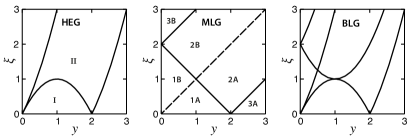
Figure 5: Domains in the momentum-energy plane in the definitions of the dielectric functions of HEG, MLG, and BLG. Here $y=q/k_{\text{F}}$ and $\xi=\omega/\epsilon_{\text{F}}$.

In this section we present in a uniform way the four studied systems. We focus on the dielectric function in the momentum-frequency plane, Fig. 5. It is closely connected to the irreducible polarization $\mathcal{P}(q,\omega)$ and to the density-density response $\chi(q,\omega)$,

$$\chi(q,\omega) =\mathcal{P}(q,\omega)+\mathcal{P}(q,\omega)v(q)\chi(q,\omega).$$ (23)

They determine the microscopic dielectric function and its inverse, respectively,

$$\varepsilon(q,\omega) =1-gv(q)\mathcal{P}(q,\omega),$$ (24)

$$\varepsilon(q,\omega)^{-1} =1+gv(q)\chi(q,\omega).$$ (25)

Here $g$ is the degeneracy factor. For the homogeneous electron gas there is only spin degeneracy, $g=g_{s}=2$, whereas for the mono- and bilayer graphene the valley degeneracy additionally appears $g=g_{s}g_{v}$. For these systems $g_{v}=2$, but it can take larger values for other systems Das Sarma et al. (2011); Basov et al. (2016). The density of states at the Fermi energy $N_{0}$ is a natural unit to measure $\mathcal{P}$ and $\chi$, because the static polarization $\mathcal{P}(q,0)$ for small values of $q$ is exactly given by this quantity, Fig. 6(a).

Figure 6: Static irreducible polarization $\mathcal{P}(q,0)$ for the four studied systems normalized at the density of states at the Fermi level $N_{0}$ (a). $N_{0}$ is given by $\rho_{\sigma}(\epsilon_{\text{F}})$ for HEG and by $\rho_{\sigma,s}(\epsilon_{\text{F}})$ for the two graphene systems, $y=q/k_{\text{F}}$ and $\xi=\omega/\epsilon_{\text{F}}$. Integrand of the $f$-sum rule for MLG (b) and BLG (c) demonstrating the divergence of the $f$-sum in these systems.

The random phase approximation for the inverse dielectric function, $\operatorname{Im}\varepsilon_{0}(q,\omega)^{-1}$ is a very important ingredient of the subsequent correlated calculations because this gives (up to the Coulomb prefactor $v(q)$) the spectral function of the screened interaction (Appendix B). A general overview of this quantity is shown in Fig. 7. It is very fortunate that for all four studied systems it can be found in analytic form facilitating numerical calculations. Below, we collect all needed formulas and additionally present the exchange self-energy, which enters Eq. (2).

In the following we express the electron density $n$, which is the central control parameter, in SI units in order to make a connection with experiment. All other quantities are expressed in atomic units. Some simplification of formulas is possible to achieve by rescaling momenta and energies by the Fermi momentum $k_{\text{F}}$ and energy $\epsilon_{\text{F}}$, respectively. This will be explicitly indicated.

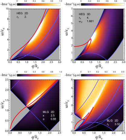
Figure 7: Imaginary part of the inverse dielectric function for the four studied systems. Red lines indicate the collective plasmonic mode. Blue lines separate different domains in the definition of polarizability such as shown in Fig. 5 and indicate removable singularities.

IV.1 2D HEG

This is probably the best studied many-body system Czachor et al. (1982); Santoro and Giuliani (1989). There is only one relevant parameter — the Wigner-Seitz radius $r_{s}$. It is given in terms of electronic density $n$ as follows:

$$a_{\text{B}}r_{s} =\left(\frac{1}{\pi n}\right)^{1/2}.$$ (26)

In the case of systems with an effective electron mass $m_{0}$ and a background dielectric constant $\kappa=4\pi\varepsilon\varepsilon_{0}$, one can redefine the Bohr radius as

$$\tilde{a}_{\text{B}} =\frac{\kappa\hbar^{2}}{m_{0}e^{2}}$$ (27)

and still have the same relation between the density and $r_{s}$. The Coulomb potential $v(q)$, the Fermi momentum $k_{\text{F}}$ and the density of states at the Fermi energy $\rho_{\sigma}(\epsilon_{\text{F}})$ in atomic units read

$$v(q) =\frac{2\pi}{q}, k_{\text{F}} =\frac{1}{\alpha_{2}r_{s}}, \rho_{\sigma}(\epsilon_{\text{F}}) =\frac{1}{2\pi},$$ (28)

where we additionally defined the constant

$$\alpha_{2} =1/\sqrt{2}.$$ (29)

Introducing scaled variables

$$y =q/k_{\text{F}}, \xi =\omega/\epsilon_{\text{F}},$$ (30)

the dielectric function $\varepsilon_{0}^{\text{R}}(k,\omega)\equiv\varepsilon_{0}^{\text{R}}(y,\xi)$ reads Stern (1967)

$$\operatorname{Re}\varepsilon_{0}^{\text{R}}(y,\xi) =1+\frac{2\alpha_{2}r_{s}}{y^{2}}\left[y+f_{r}\left(\nicefrac{{\xi}}{{y}}-y\right)-f_{r}\left(\nicefrac{{\xi}}{{y}}+y\right)\right],$$ (31)

$$\operatorname{Im}\varepsilon_{0}^{\text{R}}(y,\xi) =\frac{2\alpha_{2}r_{s}}{y^{2}}\left[f_{i}\left(\nicefrac{{\xi}}{{y}}-y\right)-f_{i}\left(\nicefrac{{\xi}}{{y}}+y\right)\right],$$ (32)

with

$$f_{r}(z) =\operatorname{sign}(z)\operatorname{\theta}(\nicefrac{{1}}{{4}}z^{2}-1)\sqrt{\nicefrac{{1}}{{4}}z^{2}-1},$$

$$f_{i}(z) =\operatorname{\theta}(1-\nicefrac{{1}}{{4}}z^{2})\sqrt{1-\nicefrac{{1}}{{4}}z^{2}}.$$

For small momentum values, the expression in brackets of Eq. (31) suffers from the precision loss. Therefore, in this limit the approximate formula

$$\operatorname{Re}\varepsilon_{0}^{\text{R}}(y,\xi) =1-\frac{qy}{\xi^{2}}, q=4\alpha_{2}r_{s}.$$ (33)

should be used entailing the small-momenta plasmon dispersion $\Omega(y)\approx\sqrt{yq}$. It can also be found analytically (see Eq. 5.54 of Ref. Giuliani and Vignale (2005)):

$$\Omega(y) =\frac{\sqrt{y}(2y+q)\sqrt{y^{4}+y^{3}q+q^{2}}}{q\sqrt{y+q}}.$$ (34)

The critical wave-vector does not have a nice analytical expression. However, one can show that $k_{c}\sim\sqrt{q}$. Notice that even though $\Omega(y)>y(y+2)$ for $y>k_{c}$ there is no plasmon above the critical vector because in reality the plasmon becomes damped by entering the continuum, where the above solution is not valid.

The $f$-sum rule reads in rescaled units

$$-\frac{2}{\pi}\int_{0}^{\infty}\mathrm{d}\xi\,\xi\operatorname{Im}\left[\frac{1}{\varepsilon^{\text{R}}(y,\xi)}\right] =\alpha_{2}r_{s}^{3}y.$$ (35)

The exchange part of the electron self-energy,

$$\Sigma_{x}(k) =-\int_{|q|<k_{\text{F}}}\frac{\mathrm{d}^{2}q}{(2\pi)^{2}}\frac{2\pi}{\kappa|\bm{\mathit{k}}-\bm{\mathit{q}}|},$$ (36)

can only be expressed Giuliani and Vignale (2005) in terms of the complete elliptic integrals (see Sec. 8. 112 in Ref. Gradshteyn and Ryzhik (2007)).

$$\bar{\Sigma}_{x}(y) =-\frac{2}{\pi}\alpha_{2}r_{s}f_{2D}(y),\qquad\bar{\Sigma}_{x}=\Sigma_{x}/\epsilon_{\text{F}},$$ (37)

$$f_{2D}(y) =\begin{cases}E(y),&y\leq 1,\\ y\left[E\left(\tfrac{1}{y}\right)-\left(1-\tfrac{1}{y^{2}}\right)K\left(\tfrac{1}{y}\right)\right],&y>1.\end{cases}$$ (38)

IV.2 3D HEG

This system also depends on a single parameter — the Wigner-Seitz radius

$$a_{\text{B}}r_{s} =\left(\frac{3}{4\pi n}\right)^{1/3}.$$ (39)

It has also been broadly studied Lundqvist (1968). The Coulomb potential $v(q)$, the Fermi momentum $k_{\text{F}}$ and the density of states at the Fermi energy $\rho_{\sigma}(\epsilon_{\text{F}})$ read in atomic units

$$v(q) =\frac{4\pi}{q^{2}}, k_{\text{F}} =\frac{1}{\alpha_{3}r_{s}}, \rho_{\sigma}(\epsilon_{\text{F}}) =\frac{1}{2\pi^{2}\alpha_{3}r_{s}},$$ (40)

where the relevant constant is defined as

$$\alpha_{3} =\left(\frac{4}{9\pi}\right)^{1/3}.$$ (41)

The dielectric function is (the Lindhard result)

$$\operatorname{Re}\varepsilon_{0}^{\text{R}}(y,\xi) =1+\frac{\alpha_{3}r_{s}}{\pi y^{3}}\left[2y+f_{r}(\nicefrac{{\xi}}{{y}}-y)-f_{r}(\nicefrac{{\xi}}{{y}}+y)\right],$$ (42)

$$\operatorname{Im}\varepsilon_{0}^{\text{R}}(y,\xi) =\frac{\alpha_{3}r_{s}}{y^{3}}\left[f_{i}\left(\nicefrac{{\xi}}{{y}}-y\right)-f_{i}\left(\nicefrac{{\xi}}{{y}}+y\right)\right],$$ (43)

with

$$f_{r}(z) =(1-\nicefrac{{1}}{{4}}z^{2})\log[(z+2)/(z-2)],$$

$$f_{i}(z) =\operatorname{\theta}(\nicefrac{{1}}{{4}}z^{2}-1)(1-\nicefrac{{1}}{{4}}z^{2}).$$

Notice a strong resemblance between the dielectric function in 2D and 3D. This is due to the fact that upper and lower continuum frequencies are the relevant parameters in both cases (Fig. 5). The shape of continuum is more complicated for MLG and BLG. However, we will see below that they likewise enter expressions for $\varepsilon_{0}^{\text{R}}(y,\xi)$.

The $f$-sum rule is particularly simple in 3D systems. This is due to the form of the Coulomb interaction proportional to $q^{-2}$ (40). Rescaling the frequency and momentum in the usual way (30) we get

$$-\frac{2}{\pi}\int_{0}^{\infty}\mathrm{d}\xi\,\xi\operatorname{Im}\left[\frac{1}{\varepsilon^{\text{R}}(y,\xi)}\right] =\omega_{p}^{2},$$ (44)

with the classical plasmon frequency ($\epsilon_{\text{F}}$ units)

$$\omega_{p} =4\sqrt{\frac{\alpha_{3}r_{s}}{3\pi}}.$$ (45)

The exchange part of the electron self-energy reads

$$\Sigma_{x}(k) =-\int_{|q|<k_{\text{F}}}\frac{\mathrm{d}^{3}q}{(2\pi)^{3}}\frac{4\pi}{|\bm{\mathit{k}}-\bm{\mathit{q}}|^{2}}.$$ (46)

Analytical expressions are well-known Giuliani and Vignale (2005)

$$\bar{\Sigma}_{x}(y) =-\frac{4}{\pi}\alpha_{3}r_{s}f_{3D}(y),\qquad\bar{\Sigma}_{x}=\Sigma_{x}/\epsilon_{\text{F}},$$ (47)

$$f_{3D}(y) =\frac{1}{2}+\frac{1-y^{2}}{4y}\log\left\lvert\frac{1+y}{1-y}\right\rvert.$$ (48)

IV.3 2D MLG

In the model approach to graphene, electronic states of the $\pi$-bands near a $K$ point of the Brillouin zone are described by the $\mathbf{k}\cdot\mathbf{p}$ equation $\hat{\mathcal{H}}_{0}\mathbf{F}(\mathbf{r})=\epsilon\mathbf{F}(\mathbf{r})$ Ando (2006); Das Sarma et al. (2011), where the Hamiltonian reads

$$\hat{\mathcal{H}}_{0} =v_{\text{F}}\begin{pmatrix}0&\hat{p}_{x}-i\hat{p}_{y}\\ \hat{p}_{x}+i\hat{p}_{y}&0\end{pmatrix}=v_{\text{F}}(\sigma_{x}\hat{p}_{x}+\sigma_{y}\hat{p}_{y}),$$ (49)

with $\hat{\mathbf{p}}=(\hat{p}_{x},\hat{p}_{y})$ being the momentum operator and $v_{\text{F}}$ the Fermi velocity (can be expressed in terms of the hopping integral and the lattice constant Basov et al. (2014), the typically adopted value is $10^{6}\,\text{m}/\text{s}=1/2.188\,\text{a.u.}$). The wave-function is then

$$\mathbf{F}_{s,\mathbf{k}}(\mathbf{r}) =|s,\mathbf{k}\rangle\frac{1}{L}e^{i\mathbf{k}\cdot\mathbf{r}}, |s,\mathbf{k}\rangle =\frac{1}{\sqrt{2}}\begin{pmatrix}e^{-i\theta_{k}}\\ s\end{pmatrix},$$ (50)

where $L^{2}$ is the area of the system, and $k_{x}=k\cos\theta_{k}$, $k_{y}=k\sin\theta_{k}$, $k=|\mathbf{k}|$. The corresponding energy dispersion reads

$$\epsilon(k) =sv_{\text{F}}k,$$ (51)

which is different from previous cases in two important ways: i) the well-known linear momentum-dependence and ii) the presence of two bands indicated by the band index $s=\pm 1$ and, as a consequence, the presence of additional matrix elements in the Coulomb operator (Fig. 8)

$$\widehat{V} =\frac{1}{2L^{2}}\sum_{\mathbf{q},\mathbf{k}_{1},\mathbf{k}_{2}}\sum_{s_{1},s_{2},s_{1}^{\prime},s_{2}^{\prime}}\langle s_{1}^{\prime},\mathbf{k}_{1}+\mathbf{q}|s_{1},\mathbf{k}_{1}\rangle\langle s_{2},\mathbf{k}_{2}-\mathbf{q}|s_{2}^{\prime},\mathbf{k}_{2}\rangle$$

$$\qquad\times\sum_{\sigma,\sigma^{\prime}}\frac{2\pi}{\kappa q}\hat{c}_{s_{1}^{\prime},\mathbf{k}_{1}+\mathbf{q},\sigma}^{\dagger}\hat{c}^{\dagger}_{s_{2},\mathbf{k}_{2}-\mathbf{q},\sigma^{\prime}}\hat{c}_{s_{2}^{\prime},\mathbf{k}_{2},\sigma^{\prime}}\hat{c}_{s_{1},\mathbf{k}_{1},\sigma}.$$ (52)

Thus, basis functions are labeled by the momentum $\mathbf{k}$, band index $s$ and spin $\sigma$. In view of the dispersion (51), the noninteracting GF is diagonal in $s$ and $\sigma$. We are interested in the electron self-energy diagonal in the band indices. Furthermore, the calculations are typically performed at finite doping (extrinsic graphene) and with dielectric function modified by the presence of substrate. We will focus on the SiO₂ substrate $\kappa=(1+\varepsilon_{\text{SiO}_{2}})/2=2.45$, consider the case of the electron doping, i.e., that the Fermi level is above the Dirac point, and follow the notations from the previous sections that

$$\kappa =4\pi\varepsilon\varepsilon_{0},$$ (53)

with $\varepsilon_{0}$ being the vacuum electric permittivity. The Fermi momentum and energy depend on the square root of the electron density

$$k_{\text{F}} =a_{\text{B}}\sqrt{\frac{4\pi n}{g}}=\frac{1}{\langle r\rangle}, \epsilon_{\text{F}} =v_{\text{F}}k_{\text{F}},$$ (54)

$g=g_{s}g_{v}$ where $g_{s}=2$ is the spin and $g_{v}=2$ is the valley degeneracy, respectively. $\langle r\rangle$ is the averaged inter-electron distance.

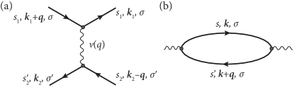
Figure 8: Diagrammatic representation of (a) the Coulomb interaction (52) and (b) the polarization bubble in MLG. The latter illustrates the appearance of the spin $g_{s}$ and band $g_{v}$ degeneracy prefactors in the dielectric function, Eqs. (56,58). The overlap matrix elements (62) are represented by shaded vertices.

The parameter characterizing the level of correlations in the system is given by the ratio of the Coulomb $E_{C}$ and the kinetic $E_{K}$ energies, as is therefore the counterpart of $r_{s}$ for the homogeneous electron gas

$$\alpha =\frac{E_{C}}{E_{K}}=\frac{1}{\kappa\,\langle r\rangle}\frac{1}{v_{\text{F}}k_{\text{F}}}=\frac{1}{\kappa v_{\text{F}}}\simeq\frac{2.188}{\kappa},$$ (55)

for instance, $\alpha=2.188$ for MLG in vacuum and $\alpha=0.875$ for the SiO₂ substrate. The dielectric function has been computed by Hwang and Das Sarma Hwang and Das Sarma (2007) and by Wunsch et al. Wunsch et al. (2006). We will use the latter form:

$$\operatorname{Re}\varepsilon_{0}^{\text{R}}(y,\xi) =1+\frac{g\alpha}{y}+g\alpha f(y,\xi)G_{r}(y,\xi),$$ (56)

$$\operatorname{Im}\varepsilon_{0}^{\text{R}}(y,\xi) =g\alpha f(y,\xi)G_{i}(y,\xi),$$ (57)

$$f(y,\xi) =\frac{1}{8}\frac{y}{\sqrt{|\xi^{2}-y^{2}|}},$$ (58)

Functions $G_{r}$ and $G_{i}$ are defined in Appendix C. The density of states at the Fermi level reads

$$\rho_{\sigma,s} =(2\pi v_{\text{F}})^{-1}.$$ (59)

The static polarizability normalized at this number is plotted in Fig 6(a). Due to the presence of infinite sea of electrons below the Dirac point, the $f$-sum rule diverges as demonstrated by Hwang, Throckmorton, and Das Sarma Hwang et al. (2018), the integrand of the $f$-sum is illustrated in Fig. 6(b).

Due to this fact, a momentum cut-off $k_{c}$ needs to be introduced for the momentum integrals. In realistic system this is not a problem because of the bands flattening due to lattice effects Trevisanutto et al. (2008). For the idealistic model that we consider here, $k_{c}$ is an explicit parameter of the theory. We adopt

$$k_{c} =y_{c}k_{\text{F}}=10k_{\text{F}}.$$ (60)

The exchange self-energy can be written in the form

$$\Sigma_{x,s}(k) =-\!\sum_{s^{\prime}=\pm 1}\!\int\!\!\frac{\mathrm{d}^{2}q}{(2\pi)^{2}}n_{\text{F},s^{\prime}}(\bm{\mathit{k}}-\bm{\mathit{q}})\frac{2\pi}{\kappa q}F_{s,s^{\prime}}(\bm{\mathit{k}},\bm{\mathit{k}}-\bm{\mathit{q}}).$$ (61)

In this equation, $F_{s_{1},s_{2}}(\mathbf{k}_{1},\mathbf{k}_{2})$ takes into account the probability for an electron with momentum $\mathbf{k}_{1}$ in the band $s_{1}$ to scatter into the state with momentum $\mathbf{k}_{2}$ in the band $s_{2}$. It depends on the relative angle $\theta_{12}$ between the two momenta,

$$\langle s_{2},\mathbf{k}_{2}|s_{1},\mathbf{k}_{1}\rangle =\tfrac{1}{2}(1+s_{1}s_{2}e^{i\theta_{12}}),$$ (62)

$$F_{s_{1},s_{2}}(\mathbf{k}_{1},\mathbf{k}_{2})=|\langle s_{2},\mathbf{k}_{2}|s_{1},\mathbf{k}_{1}\rangle|^{2} =\tfrac{1}{2}(1+s_{1}s_{2}\cos\theta_{12}).$$ (63)

Using the Fermi energy and momentum units, dividing into intrinsic (present in pristine graphene) and extrinsic (due to carriers injection by doping or gating) contributions, shifting by the constant so that the self-energy is zero at the Dirac point ($\Sigma_{x,\pm 1}(0)=0$) we obtain for Eq. (61)

$$\bar{\Sigma}_{x,s}(y) =\bar{\Sigma}_{x,s}^{\text{int}}(y)+\bar{\Sigma}_{x,s}^{\text{ext}}(y)+\frac{\alpha}{2}(1+y_{c}),$$ (64)

with

$$\bar{\Sigma}_{x,s}^{\text{int}}(y) =-\frac{\alpha y_{c}}{\pi}\left[\frac{\pi}{2}-sg\left(\frac{y}{y_{c}}\right)\right],$$ (65)

$$\bar{\Sigma}_{x,s}^{\text{ext}}(y) =-\frac{\alpha}{\pi}\Big{[}f_{2D}(y)+sh(y)\Big{]}.$$ (66)

The function $f_{2D}(y)$ has already been defined for 2D HEG (38). The former intrinsic part results from the integration over the $s^{\prime}=-1$ band from zero to the momentum cut-off $k_{c}=y_{c}k_{\text{F}}$. Functions $h(y)$ and $g(y)$ have a representation (correcting $g(y)$ in the original derivation by Hwang, Hu and Das Sarma Hwang et al. (2007)):

$$h(y) =y\begin{dcases}\tfrac{\pi}{4}\log\tfrac{4}{ye^{1/2}}-\int_{0}^{y}\!\tfrac{\mathrm{d}x}{x^{3}}\left[K(x)-E(x)-\tfrac{\pi x^{2}}{4}\right]&y\leq 1,\\ \int_{0}^{1/y}\!\mathrm{d}x\,[K(x)-E(x)]&y>1;\end{dcases}$$ (67)

$$g(x) =\frac{1}{4}\int_{0}^{1}\!\mathrm{d}y\int_{0}^{2\pi}\!\mathrm{d}\theta\frac{x-y\cos\theta}{\sqrt{x^{2}+y^{2}-2xy\cos\theta}}$$

$$\qquad=\frac{\pi}{2}\operatorname{Re}\left\{{}_{3}F_{2}\left(-\tfrac{1}{2},\tfrac{1}{2},\tfrac{1}{2};1,\tfrac{3}{2};\tfrac{1}{x^{2}}\right)\right\}.$$ (68)

IV.4 2D BLG

Consider now two parabolic energy bands

$$\epsilon(k) =sk^{2}/(2m_{0}).$$ (69)

Unlike MLG, the dispersion is an idealization of several materials with different number of valleys $g_{v}$ and with large flexibility in the properties control with the help of doping and the background dielectric constant. Here we focus on the $g_{v}=2$ case pertinent to the bilayer graphene (a minimal two-band model for the Bernal $AB$ stacking Kotov et al. (2012)). We have the following relations determining the Fermi energy and momentum, and the Wigner-Seitz radius Sensarma et al. (2010)

$$\frac{k_{\text{F}}}{a_{\text{B}}} =\sqrt{\frac{4\pi n}{g_{s}g_{v}}}, \epsilon_{\text{F}} =\frac{k_{\text{F}}^{2}}{2m_{0}}, r_{s} =\frac{gm_{0}}{\kappa k_{\text{F}}}, \rho_{\sigma,s}(\epsilon_{\text{F}}) =\frac{m_{0}}{2\pi}.$$ (70)

One may also define the Wigner-Seitz radius as the ratio of two energies

$$\tilde{r}_{s} =\frac{E_{C}}{E_{K}}=\frac{1}{\kappa\langle r\rangle}\frac{2m_{0}}{k_{\text{F}}^{2}}=\frac{m_{0}}{\kappa}\frac{g_{s}g_{v}a_{\text{B}}}{(4\pi n)^{1/2}}, a_{\text{B}}\langle r\rangle=\left(\frac{1}{\pi n}\right)^{1/2}.$$

Sensarma, Hwang and Das Sarma Sensarma et al. (2010) derived the polarizability of this system separating the intra(inter)-band contributions $\Pi=\Pi_{1}+\Pi_{2}$. The former originates from the intraband ($s=s^{\prime}$) and the latter from interband ($s=-s^{\prime}$) transitions, Fig. 8(b),

$$\Pi_{1}(y,\xi) =\frac{1}{\pi}\int_{0}^{1}\!\mathrm{d}x\int_{-\pi}^{\pi}\!\mathrm{d}\phi\,\frac{x}{\xi+i\eta-2xy\cos(\phi)-y^{2}}$$

$$\quad\times\left[1-\frac{y^{2}\sin^{2}(\phi)}{x^{2}+2xy\cos(\phi)+y^{2}}\right],$$ (71)

$$\Pi_{2}(y,\xi) =-\frac{1}{\pi}\int_{0}^{1}\!\mathrm{d}x\int_{-\pi}^{\pi}\!\mathrm{d}\phi\,\frac{x}{\xi+i\eta+2x^{2}+2xy\cos(\phi)+y^{2}}$$

$$\quad\times\frac{y^{2}\sin^{2}(\phi)}{x^{2}+2xy\cos(\phi)+y^{2}}.$$ (72)

The retarded polarizability is given by

$$\operatorname{Re}\mathcal{P}(y,\xi) =\operatorname{Re}\Pi(y,\xi)+\operatorname{Re}\Pi(y,-\xi),$$ (73)

$$\operatorname{Im}\mathcal{P}(y,\xi) =\operatorname{Im}\Pi(y,\xi)-\operatorname{Im}\Pi(y,-\xi).$$ (74)

$\Pi_{1}$ is fully defined in the paper Sensarma et al. (2010). There are, however, some misprints in the extrinsic part that are corrected here in Appendix D. The dielectric function is given by

$$\varepsilon_{0}^{\mathrm{R}}(y,\xi) =1-\frac{r_{s}}{y}\mathcal{P}(y,\xi).$$ (75)

Th static polarizability was derived by Hwang and Das Sarma Hwang and Das Sarma (2008b) and is plotted here for comparison with other systems in Fig. 6(a). The $f$-sum rule diverges for this system for the same reasons as for MLG. The integrand of the $f$-sum is illustrated in Fig. 6(c). The exchange self-energy is the same as for MLG (66).

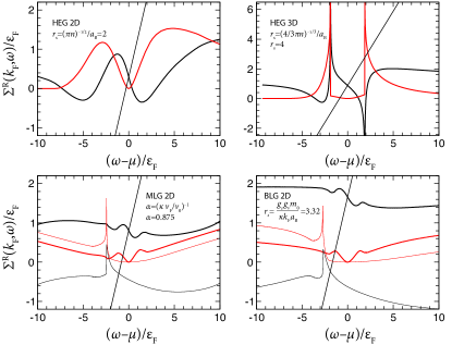
Figure 9: Solution of the Dyson equation for the Fermi level $k=k_{\text{F}}$. Intersection of straight line $y=\omega-\epsilon_{\text{F}}-\Delta\mu$ and $y=\operatorname{Re}\Sigma^{\text{R}}(k_{\text{F}},\omega)$ (thick black curve) yields the real part of quasiparticle energy. The chemical potential shift $\Delta\mu$ is selected (see Appendix E) as to have the imaginary part zero in accordance with the Fermi liquid assumption. Red curves stand for $\nicefrac{{1}}{{2}}\Gamma(k_{\text{F}},\omega)=-\operatorname{Im}\Sigma^{\text{R}}(k_{\text{F}},\omega)$. In the case of MLG and BLG thick/thin curves correspond to $\Sigma^{\mathrm{R}}_{s=\pm 1}(k_{\text{F}},\omega)$.

IV.5 $G_{0}W_{0}$ calculations

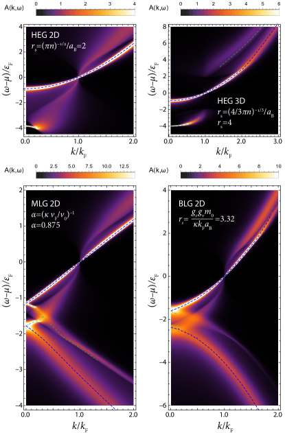
Figure 10: The electron spectral function from the solution of the Dyson equation with self-energy in $G_{0}W_{0}$ approximation. For MLG and BLG, the spectral function is a matrix in the band indices, the trace of it is shown here.

Before presenting calculations with vertex functions, we overview the electron self-energy in the simplest $G_{0}W_{0}$ approximation, Eq. (14). The self-energy is depicted in Fig. 9, the respective electron spectral function

$$A(k,\omega) =-2\operatorname{Im}G^{\text{R}}(k,\omega)$$ (76)

is shown in Fig. 10.

HEG

systems have a long history of studies: Lundqvist Lundqvist (1968), Hedin Hedin (1965) and self-consistent $GW$ calculations by von Barth and Holm von Barth and Holm (1996); Holm and von Barth (1998) in 3D and Giuliani and Quinn Giuliani and Quinn (1982), Santoro and Giuliani Santoro and Giuliani (1989), Zhang and Das Sarma Zhang and Das Sarma (2005), Lischner et al. Lischner et al. (2014) in 2D. Because of the way how 2D HEG is engineered (its properties can be tuned by doping, the electron concentration), it is easy to go to strongly correlated regime and still have a homogeneous system. Therefore, correlations beyond $G_{0}W_{0}$ have been included almost from the beginning. Thus, Santoro and Giuliani included the many-body local fields $G_{\pm}$ in the calculation of screening and employed the plasmon-pole approximation. This yields the self-energy resembling the 3D case and results in a more pronounced plasmon peak as compared to the $G_{0}W_{0}$ calculations.

Graphene

There are two peculiarities in the case of MLG and BLG systems. (i) The electron dispersion and self-energies additionally carry the valley index $s$ resulting in the following modification of Eq. (14):

$$\Sigma_{GW,s}^{<}(k,\omega) =2i\pi\sum_{s^{\prime}=\pm 1}\int_{0}^{q_{1}\leq k_{c}}\frac{\mathrm{d}^{2}q_{1}}{(2\pi)^{2}}\int_{0}^{\infty}\!\mathrm{d}\nu_{1}\,F_{s,s^{\prime}}(\bm{\mathit{k}};\bm{\mathit{k}}_{1})$$

$$\qquad\times n_{\text{F},s^{\prime}}(k_{1})C(q_{1},\nu_{1})\operatorname{\delta}(\omega+\nu_{1}-\epsilon_{1}),$$ (77)

where the scattering matrix element $F_{s,s^{\prime}}$ is given by Eq. (63). (ii) Due to the presence of an infinite electron sea below the Dirac point the diverging momentum integrals need to be regularized with the help of cut-off (60). One can also introduce a frequency cut-off without compromising the accuracy.

Hwang and Das Sarma Hwang and Das Sarma (2008a) and Polini et al. Polini et al. (2008) performed calculations for MLG, more extensive investigations for a range of momenta are in Refs. Bostwick et al. (2010); Walter et al. (2011); Carbotte et al. (2012); Das Sarma and Hwang (2013). Respective calculations for BLG have been performed by Sensarma, Hwang and Das Sarma Sensarma et al. (2011) and Sabashvili et al. Sabashvili et al. (2013).

V $\Sigma_{a\bar{a}}$: scattering accompanied by the generation of a $ph$-pair with exchange

$\Sigma_{a\bar{a}}$ is the main objective of this work. It describes the simplest second-order process in which a particle scatters giving rise to an additional particle-hole pair in the final state, Fig. 4. It is obtained by gluing two half-diagrams $D^{(a)}$ with a permutation, and therefore does not lead to a PSD spectral functions on its own. However, the inclusion of an unpermuted configuration gives rise to $\Sigma_{aa}$ restoring the PSD property. In this work $\Sigma_{a\bar{a}}$ is computed according to Eq. (20), which needs some modifications in the case of graphene in order to account for the band indices. After discussing this technical point in Sec. V.1, we consider the influence of screening on $\Sigma_{a\bar{a}}$ in Sec. V.2, the cancellations between $\Sigma_{aa}$ and $\Sigma_{a\bar{a}}$ in the asymptotic regime in Sec. V.3, and finally focus on the resulting quasiparticle properties in Sec. V.4.

V.1 Computation for MLG and BLG systems

In the case of graphene, Eq. (20) additionally gets a sum over three internal band indices and an additional factor, which is a product of the four wave-function overlaps,

$$F_{s_{0},s_{1}s_{2}s_{3}}(\mathbf{k}_{0};\mathbf{k}_{1},\mathbf{k}_{2},\mathbf{k}_{3})=\langle s_{0},\mathbf{k}_{0}|s_{1},\mathbf{k}_{1}\rangle\langle s_{1},\mathbf{k}_{1}|s_{3},\mathbf{k}_{3}\rangle\\ \times\langle s_{3},\mathbf{k}_{3}|s_{2},\mathbf{k}_{2}\rangle\langle s_{2},\mathbf{k}_{2}|s_{0},\mathbf{k}_{0}\rangle=\frac{1}{8}\Big{\{}1+\sum_{i<j}s_{i}s_{j}\cos\theta_{ij}\\ +s_{0}s_{1}s_{2}s_{3}\cos(\theta_{01}+\theta_{32})\Big{\}},$$ (78)

where $\theta_{ij}$ is the angle between the respective momenta. The second-order exchange then takes a form

$$\Sigma_{2x,s}^{<}(k,\omega)=-2i\pi\!\sum_{s_{1},s_{2},s_{3}}\!\iint\!\mathrm{d}(\Omega_{1,2})\,F_{s,s_{1}s_{2}s_{3}}(\bm{\mathit{k}};\bm{\mathit{k}}_{1},\bm{\mathit{k}}_{2},\bm{\mathit{k}}_{3})\\ v(q_{1})v(q_{2})n_{\text{F}}(\epsilon_{1})n_{\text{F}}(\epsilon_{2})\bar{n}_{\text{F}}(\epsilon_{3})\delta(\omega-\epsilon_{1}-\epsilon_{2}+\epsilon_{3}),$$ (79)

where the momenta are defined by Eq. (10) and depicted in Fig. 3(a). It should be noted that our original PSD construction was formulated for the systems free of the ultra-violet divergences. Here it is applied graphene, for which the momentum integrals are regularized with the wave-vector cutoff $k_{c}$ with the justification that the regularization can be implemented on the level of Hamiltonian.

V.2 $\Sigma_{2x}$ results for 3D HEG

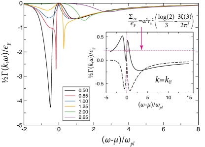
Figure 11: $\Sigma_{2x}$ at different momentum values. The inset shows the real self-energy part (solid line) obtained from the Hilbert transform of $\Gamma_{a\bar{a}}(k_{\text{F}},\omega)$. Its on-shell value ($\epsilon_{2x}(k_{\text{F}},\mu)=0.204976$) has only 2.4% deviation from the indicated analytic result (0.210073).

Corresponding imaginary part is plotted in Fig. 11. The Hilbert transform (Appendix A) yields the real part. On the inset we see a very good agreement of our numerical result with the analytical expression

$$\epsilon_{2x}=\operatorname{Re}\Sigma_{2x}(k_{\text{F}},\mu)/\epsilon_{\text{F}}=\frac{\alpha^{2}r_{s}^{2}}{2\pi^{2}}\left(\frac{2\pi^{2}}{3}\ln(2)-3\zeta(3)\right),$$

that is known due to the calculations of Glasser and Lamb Glasser and Lamb (2007) and Ziesche Ziesche (2007) or from the second-order correction to the total energy computed by Onsager et al. Onsager et al. (1966). According to the Hugenholtz-van Hove-Luttinger-Ward theorem they are equal. Despite claims Isihara and Ioriatti (1980), it seems impossible to get the respective expression in analytic form for 2D HEG Glasser (2018).

Going away from $k=k_{\text{F}}$, the self-energy first develops an additional sharp peak in the vicinity of $\omega=\mu$ as seen for $k=0.85k_{\text{F}},1.25k_{\text{F}}$, which eventually becomes smeared out, Fig. 12. This is a rather disturbing fact because large negative values need to be compensated by $\Sigma_{aa}$, which does not have any singularities in this energy range. Thus, a better understanding of the origin of this peak is needed.

Figure 12: The momentum- and energy-resolved scattering rate computed with the bare Coulomb interaction for $r_{s}=4$. It is negative and possesses a strong peak due to the small-momentum forward scattering. Screening greatly reduces its magnitude, whereas $\Sigma_{aa}$ compensates for the negative values.

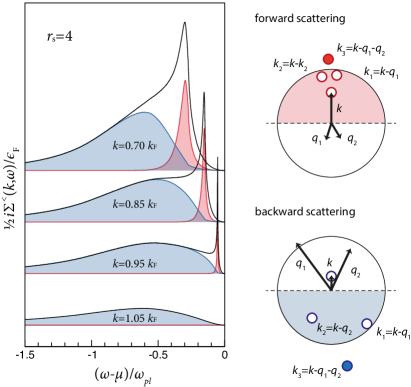
Figure 13: $\Sigma_{2x}$ at different momentum values resolved with respect of forward (red) and backward (blue) scattering mechanisms. For a hole in the center of the Fermi sphere $k\ll k_{\text{F}}$, backward scattering dominates, while for a hole close to the Fermi surface $k\approx k_{\text{F}}$ forward scattering with a small momentum transfer gives rise to a sharp peak.

In Fig. 13 we re-plot $i\Sigma_{a\bar{a}}^{<}$ computed with bare Coulomb interaction for different momentum values paying attention to the kinematic aspects. In particular, we are interested in the distribution of momenta carried by the two interaction lines $\bm{\mathit{q}}_{1,2}$ and, correspondingly, in the configuration of the final state formed by two holes with momentum $\bm{\mathit{k}}_{1,2}=\bm{\mathit{k}}-\bm{\mathit{q}}_{1,2}$ and a particle $\bm{\mathit{k}}_{3}=\bm{\mathit{k}}-\bm{\mathit{q}}_{1}-\bm{\mathit{q}}_{2}$, Fig. 4. It is, of course, difficult to depict all the multitude of possibilities taking place in our Monte Carlo simulations. However, a useful classification of the involved physical processes can be found: we distinguish the forward and the backward scatterings scenarios. The former is defined as a process in which $\bm{\mathit{q}}_{1}$ and $\bm{\mathit{q}}_{2}$ are anti-parallel to the initial hole momentum, i. e., the scalar products $(\bm{\mathit{k}},\bm{\mathit{q}}_{1})$ and $(\bm{\mathit{k}},\bm{\mathit{q}}_{2})$ are negative. In this case the initial hole state with momentum $k$ gets transformed into two-hole states with momenta in the same Fermi hemisphere (red). For the backward scattering both of these products are positive and, correspondingly, the final hole states are in the opposite hemisphere. From the scheme depicted in Fig. 13 it becomes evident that there is a very limited phase space for the forward mechanism if the initial hole is in the vicinity of Fermi sphere, $k\rightarrow k_{\text{F}}$. In order to guarantee that $k_{1,2}\leq k_{\text{F}}$ and $k_{3}>k_{\text{F}}$ the interaction momenta $\bm{\mathit{q}}_{1,2}$ must be small and almost collinear with $\bm{\mathit{k}}$. As a result we have a “hot-spot” in the momentum space where all the permitted configurations contribute in a very narrow energy interval giving rise to a pronounced forward peak. If the initial state is closer to the center of Fermi sphere, there are less restrictions on the possible scattering angles. Therefore, the forward peak broadens, and for larger energy transfers the backward scattering dominates. It is interesting to notice that the mixed mechanism, i. e., where one hole is in the forward and another in the backward direction, has a rather small contribution and takes place at intermediate energies.

From our analysis follows that small momentum transfers $q_{1,2}$ are important for the appearance of the forward peak. In this regime the Coulomb interaction is screened by plasmons suggesting that the inclusion of screening may reduce the peak. Therefore, we performed three calculations for $k=0.85k_{\text{F}}$ with i) bare Coulomb lines, ii) with only plasmon screening, and iii) using the fully screened RPA $W_{0}$. They indeed demonstrate that the plasmonic contribution to $\Sigma_{a\bar{a}}$ is essential for compensating the singularity in the bare Coulomb term (Fig. 14). Notice that they both appear with the same sign because the interactions enter quadratically in the expression for $\Sigma_{a\bar{a}}$. As a result, a smooth frequency dependence free of any singularities is obtained for the sum of all contributions.

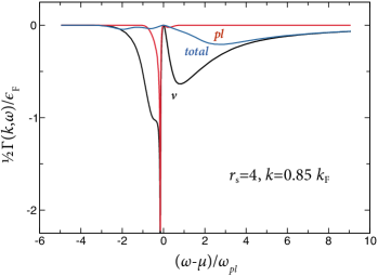
Figure 14: $\Sigma_{a\bar{a}}$ computed with full RPA screenings $W_{0}$ (total), plasmon pole approximation for $W_{0}$ ($pl$), and bare Coulomb interaction ($v$). Screening, which is operative at small momentum transfers, is responsible for the cancellation of singularity.

V.3 Cancellations between $\Sigma_{aa}^{<}$ and $\Sigma_{a\bar{a}}^{<}$ in the asymptotic regime

The asymptotic regime $\omega\rightarrow\pm\infty$ is important because there $\Sigma_{aa}$ approaches zero, and a failure of the PSD construction would be evident. It is convenient to perform derivations using scaled variables $\bm{\mathit{x}}_{i}=\bm{\mathit{k}}_{i}/k_{\text{F}}$, $\bm{\mathit{y}}_{i}=\bm{\mathit{q}}_{i}/k_{\text{F}}$, $\zeta=\omega/\epsilon_{\text{F}}$.

3D HEG

The $G_{0}W_{0}$ self-energy scales in the high-frequency limit Pavlyukh et al. (2013) as

$$\tfrac{i}{2}\overline{\Sigma}_{aa}^{>}(x,\zeta) \equiv\tfrac{i}{2}\Sigma_{aa}^{>}(k/k_{\text{F}},\omega/\epsilon_{\text{F}})/\epsilon_{\text{F}}\stackrel{{\scriptstyle\zeta\rightarrow\infty}}{{\longrightarrow}}c_{1}\frac{\alpha_{3}^{2}r_{s}^{2}}{\zeta^{3/2}},$$ (80)

$$c_{1} =\frac{16\sqrt{2}}{3\pi}.$$ (81)

Conversely, this determines the short-time behavior of the electron GF. Unexpectedly, Vogt et al. Vogt et al. (2004) have demonstrated that the second-order exchange $\Sigma_{2x}$ asymptotically scales in the same way, but with an additional $-\nicefrac{{1}}{{2}}$ prefactor. This result can be further generalized and derived as follows.

Figure 15: Asymptotic behavior of $i\Sigma_{aa}^{>}$ (only $p$-$h$ excitations) and $-i\Sigma_{2x}^{>}$ for large momentum values plotted on the logarithmic scale. The latter quantity is negative and therefore is multiplied with $-1$. A scheme on the right illustrates momentum configuration of $p\rightarrow p+p+h$ scattering at large energy and momentum transfer, i. e. in the asymptotic regime $\omega\gg k^{2}/2\gg\epsilon_{\text{F}}$. In this limit $k_{3}\ll k$ and can be integrated over.

The generalization concerns the fact that in the high frequency limit, the screening is not important and the screened interactions in the expression for $\Sigma_{a\bar{a}}$ can be replaced with the bare Coulomb, i. e., $W^{--}(q_{1},\omega-\epsilon_{1})\rightarrow v(q_{1})$, $W^{++}(q_{2},\omega-\epsilon_{2})\rightarrow v(q_{2})$. This means that $\Sigma_{a\bar{a}}$ asymptitocally behaves as $\Sigma_{2x}$. Using the momenta flow as in Fig. 3(a), the second-order exchange reads

$$\tfrac{i}{2}\overline{\Sigma}_{2x}^{>}(x,\zeta) =-\frac{\alpha_{3}^{2}r_{s}^{2}}{\pi^{3}}\iint\frac{\mathrm{d}^{3}\bm{\mathit{y}}_{1}}{y_{1}^{2}}\frac{\mathrm{d}^{3}\bm{\mathit{y}}_{2}}{y_{2}^{2}}\,\bar{n}_{\text{F}}(x_{1})\bar{n}_{\text{F}}(x_{2})n_{\text{F}}(x_{3})$$

$$\qquad\qquad\times\delta(\zeta-\epsilon_{1}-\epsilon_{2}+\epsilon_{3}).$$ (82)

In the asymptotic case $\zeta\gg x^{2}/2\gg 1$ we have $x_{3}\ll x_{1,2}$. We change the variables

$$\bm{\mathit{y}}_{1,2}=\frac{1}{2}\bm{\mathit{x}}\pm\bm{\mathit{z}}=\bm{\mathit{x}}_{2,1}$$

and integrate over $\bm{\mathit{x}}_{3}$ within the Fermi sphere (from the scheme in Fig. 15 it is evident that to a good approximation the integrand is independent of $x_{3}$) yielding the $4\pi/3$ prefactor to the following remaining integral

$$\tfrac{i}{2}\overline{\Sigma}_{2x}^{>}(x,\zeta) \approx-\frac{4\alpha_{3}^{2}r_{s}^{2}}{3\pi^{2}}\int\!\frac{\mathrm{d}^{3}\bm{\mathit{z}}}{\big{|}\frac{1}{2}\bm{\mathit{x}}-\bm{\mathit{z}}\big{|}^{2}\big{|}\frac{1}{2}\bm{\mathit{x}}+\bm{\mathit{z}}\big{|}^{2}}\delta\big{(}\zeta-\frac{1}{2}x^{2}-2z^{2}\big{)}$$

$$=-\frac{8\alpha_{3}^{2}r_{s}^{2}}{3\pi}\frac{\tanh^{-1}\left(\frac{x\sqrt{2\zeta-x^{2}}}{\zeta}\right)}{\zeta x}$$

$$=-\frac{8\sqrt{2}}{3\pi}\frac{\alpha_{3}^{2}r_{s}^{2}}{\zeta^{3/2}}+\mathcal{O}(x^{2}).$$ (83)

In the last step, we exploit the high-frequency assumption $\zeta\gg x^{2}/2$ and perform a series expansion over $x$ to get the conjectured scaling $i\overline{\Sigma}_{2x}^{>}(x,\zeta)\stackrel{{\scriptstyle\zeta\rightarrow\infty}}{{\longrightarrow}}c_{2}\alpha_{3}^{2}r_{s}^{2}\zeta^{-3/2}$. The scaling is verified numerically in Fig. 15 confirming that the constant $c_{2}$ computed from Eq. (83) is momentum-independent. It is important, however, that $c_{2}=-\frac{1}{2}c_{1}$ ensuring the PSD property in the high-frequency limit.

2D HEG

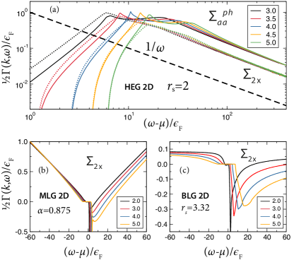
Figure 16: Top: asymptotic behavior of the rate functions $i\Sigma_{aa}^{>}$ (only $p$-$h$ excitations) and $-i\Sigma_{2x}^{>}$ for large momentum values plotted on the logarithmic scale for 2D HEG. As in the 3D HEG, they posses the $c_{1,2}/\omega$ scaling, respectively, with $c_{2}=-1/2c_{1}$. In panels (b,c) the rate function of the two graphene systems is plotted for different momentum values. There is no universal scaling.

The derivation follows the same line:

$$\tfrac{i}{2}\overline{\Sigma}_{2x}^{>}(x,\zeta) \approx-2\int\!\frac{\mathrm{d}^{2}\bm{\mathit{z}}}{\big{|}\frac{1}{2}\bm{\mathit{x}}-\bm{\mathit{z}}\big{|}\big{|}\frac{1}{2}\bm{\mathit{x}}+\bm{\mathit{z}}\big{|}}\delta\big{(}\zeta-\frac{1}{2}x^{2}-2z^{2}\big{)}$$

$$=-\frac{4}{|\zeta-x^{2}|}K\left(\frac{x\sqrt{x^{2}-2\zeta}}{\zeta-x^{2}}\right)$$

$$=-\frac{2\pi}{\zeta}+\mathcal{O}(x^{2}),$$ (84)

where $K$ is a complete elliptic integral. As in the case of the 3D HEG, there is a universal (momentum-independent) asymptotic scaling, see Fig. 16(a), and the ratio of the prefactors is the same. This is yet another exact analytical statement about the second-order self-energy.

Graphene systems

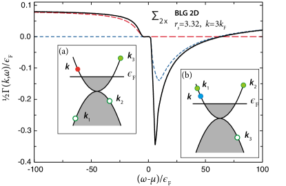
Figure 17: Second-order exchange in the BLG system for $k=3k_{\text{F}}$. Besides common scattering channels, the $\omega\rightarrow\infty$ behavior is dominated by a processes (blue line) with one hole in the lower band, $s_{3}=-1$ (inset b), for $\omega\rightarrow-\infty$ a mechanism with 2 holes in the lower band $s_{1}=s_{2}=-1$ is dominating (inset a).

The situation is much more complex in the case of graphene, Fig. 16(b,c). Besides the usual scattering processes considered above, $\Sigma_{a\bar{a}}$ contains processes in which particles change the band, Fig. 17. For instance, for $k>k_{\text{F}}$ our calculations indicate that $\Sigma_{2x}(k,\omega)$ is dominated by the process with $s_{3}=-s_{1}=-s_{2}=1$ for $\omega<0$, and with $-s_{3}=s_{1}=s_{2}=1$ for $\omega>0$, see Eq. (78). This leads to the scattering rates that do not tend to zero as $\omega\rightarrow\pm\infty$. They are cut-off dependent and should be treated as in the case of the first-order exchange.

V.4 Quasiparticle properties

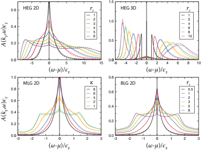
Figure 18: Electron spectral functions for quasiparticle states at the Fermi surface ($k=k_{\text{F}}$) for different interaction strengths. Dashed lines stand for the $G_{0}W_{0}$ results, full lines — additionally include $\Sigma_{a\bar{a}}$.

All four considered systems possess very distinct spectral functions. In the vicinity of the quasiparticle peak they can be represented in the Lorentzian form

$$A(k,\omega) =Z_{qp}\frac{1/\tau(k)}{(\omega-\epsilon_{qp}(k))^{2}+1/(2\tau(k))^{2}},$$ (85)

where the peak position $\epsilon_{qp}(k)$, the inverse life-time $1/\tau(k)$, and the quasiparticle renormalization factor $Z_{qp}$ can be determined by solving the Dyson equation with the given retarded self-energy operator (see Sec. 13.1 in Ref. Stefanucci and van Leeuwen (2013)). In general, one has to take care whether the spectral density can really be written in this form with finite $Z_{qp}$. For instance, this might be not the case in undoped graphene González et al. (1999); Barnes et al. (2014), or 2D systems with short-range repulsive interactions Chubukov (1993), but is the case for the systems considered here. As can be seen from Fig. 18, the second-order self-energy has a rather small impact on the shape of quasiparticle peak and its satellites. Therefore, in order to quantify the effect we compute the quasiparticle peak strength:

$$Z_{qp}(k)=\left(1-\frac{\partial}{\partial\omega}\left.\operatorname{Re}\Sigma^{\text{R}}(k,\omega)\right|_{\omega=\epsilon_{qp}(k)}\right)^{-1}.$$ (86)

We further characterize the quasiparticle dispersion in terms of the effective mass:

$$\frac{1}{m^{*}}=\frac{1}{k_{\text{F}}}\left.\frac{\mathrm{d}\epsilon_{qp}(k)}{\mathrm{d}k}\right|_{k=k_{\text{F}}},$$ (87)

and the Fermi velocity (for MLG)

$$v_{\text{F}}^{*}=\left.\frac{\mathrm{d}\epsilon_{qp}(k)}{\mathrm{d}k}\right|_{k=k_{\text{F}}}.$$ (88)

Finally, the inverse quasiparticle life-time is computed,

$$\tau(k)^{-1} =Z_{qp}(k)\Gamma(k,\epsilon_{qp}(k)),$$ (89)

$$\tfrac{1}{2}\Gamma(k,\omega) =-\operatorname{Im}\Sigma^{\text{R}}(k,\omega).$$ (90)

We are mostly interested in the correlated regime $r_{s}\gg 1$. However, the asymptotic results $r_{s}\rightarrow 0$ are also shown when available in order to demonstrate that they are valid in a rather very narrow density interval. Our main comparison is with three classes of theories. As benchmarks for the homogeneous electron gas, the quantum Monte-Carlo results of Holzmann et al. Holzmann et al. (2009) (2D) and Holzmann et al. (2011) (3D) are used. The second class of methods has been advocated by Giuliani and co-workers: Ref. Asgari et al. (2005) (2D) and Ref. Simion and Giuliani (2008) (3D). They improve upon $G_{0}W_{0}$ by using parameterized data from QMC calculations in terms of the charge and the spin static local fields factors, $G_{+}(q)$ and $G_{-}(q)$, respectively. In their method, the self-energy is in the $GW$ form, however, the screened interaction is replaced by the Kukkonen-Overhauser effective interaction Kukkonen and Overhauser (1979). Furthermore, a diagrammatic approach based on the Bethe-Salpeter equation for the improved screened interaction by Kutepov and Kotliar Kutepov and Kotliar (2017) is also used for comparison. Unfortunately, none of these theories are available for graphene systems.

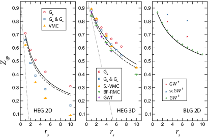
Figure 19: Quasiparticle renormalization factor for $k=k_{\text{F}}$ and different interaction strengths: $\Sigma_{G_{0}W_{0}}$—dashed, $\Sigma_{G_{0}W_{0}}+\Sigma_{a\bar{a}}$—solid lines. For 2D HEG, the variational Monte-Carlo (VMC) results are taken from Ref. Holzmann et al. (2009), and the VMC calculations using Slater-Jastrow (SJ) wave-functions and backflow (BF) reptation Monte-Carlo (RMC) for 3D HEG from Ref. Holzmann et al. (2011). $G_{+}(q)$ and $G_{+}(q)\&G_{-}(q)$ denote methods based on the local structure factors from Ref. Asgari et al. (2005) (2D) and Ref. Simion and Giuliani (2008) (3D). $GW\Gamma$ is a scheme D of Ref. Kutepov and Kotliar (2017), it includes the first-order vertex function in the finite temperature formalism. For BLG, $\dagger$ — Ref. Sabashvili et al. (2013), $\ddagger$ —  Ref. Sensarma et al. (2012).

We start by compiling the data for homogeneous electron gases in 2D and 3D and the bilayer graphene. In these systems $r_{s}$ is the relevant parameter that can be controlled by doping or other means. In MLG, there is only an indirect possibility to control $\alpha$ by changing the background dielectric constant and $\kappa$. This system will be considered later.

$r_{s}$ as a control parameter

In Fig. 19 the quasiparticle renormalization factor $Z_{qp}(k_{\text{F}})$ as a function of the density parameter $r_{s}$ is shown. As expected, the agreement between different methods deteriorates with increasing $r_{s}$, moreover the quantum Monte-Carlo results are not available for BLG. Therefore, it is hard to say with absolute certainty what is the “right” value. On the positive side, we see a very nice convergence of all methods towards the linear asymptote

$$Z_{qp} =1-\left(\frac{1}{2}+\frac{1}{\pi}\right)\alpha_{2}r_{s}, 2D$$ (91)

$$Z_{qp} =1-\frac{c}{\pi^{2}}\alpha_{3}r_{s}, 3D.$$ (92)

with $c=-\int_{0}^{\pi/2}\log(1-x\cot x)\,\mathrm{d}x\approx 3.353$. The 3D result is by Daniel and Vosko Daniel and Vosko (1960), and the 2D asymptote together with temperature corrections is due to Galitski and Das Sarma Galitski and Das Sarma (2004). For BLG, the effect of $\Sigma_{a\bar{a}}$ is negligible, and our calculations accurately reproduce the corrected results of Sensarma et al. Sensarma et al. (2012), whereas the one-shot and the self-consistent $GW$ calculations of Sabashvili et al. Sabashvili et al. (2013) deviate. For HEG in 2D and 3D, the inclusion of $\Sigma_{a\bar{a}}$ slightly increases the value of $Z_{qp}$. It is interesting to notice that the same trend is observed when the charge local field factor $G_{+}(q)$ is included. For HEG 2D, the additional inclusion of both local fields reduces $Z_{qp}$ in agreement with variational MC calculations. At variance, for HEG 3D the effect of the spin local field is less pronounced Simion and Giuliani (2008), and is nearly the same as in our calculations with $\Sigma_{a\bar{a}}$. The effect of the vertex function in Ref. Kutepov and Kotliar (2017) is rather small, therefore, it would be interesting if these calculations could be extended towards larger $r_{s}$, where even variational and backflow reptation MC results are in disagreement.

Less accurate are the predictions of different theories for the effective mass, Fig. 20. The situation gets complicated due to different methods of its determination adopted in literature Zhang and Das Sarma (2005); Asgari et al. (2005). In order to avoid any ambiguities, the masses in our approach are obtained per definition, that is by solving the Dyson equation for $\epsilon_{qp}(k)$ and using Eq. (87), and not by using the self-energy representation

$$\frac{1}{m^{*}}=\frac{Z_{qp}^{-1}}{1+\frac{1}{k_{\text{F}}}\left.\frac{\mathrm{d}\operatorname{Re}\Sigma^{\text{R}}(k,\epsilon_{\text{F}})}{\mathrm{d}k}\right|_{k=k_{\text{F}}}}.$$ (93)

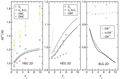
Figure 20: Effective mass for different interaction strengths: $\Sigma_{G_{0}W_{0}}$—dashed, $\Sigma_{G_{0}W_{0}}+\Sigma_{a\bar{a}}$—solid lines. For 2D HEG, the variational Monte-Carlo (VMC) results are taken from Ref. Holzmann et al. (2009), and the DMC calculations from Ref. Drummond and Needs (2009). $G_{+}(q)$ and $G_{+}(q)\&G_{-}(q)$ denote methods based on the local structure factors from Ref. Asgari et al. (2005) (2D) and Ref. Simion and Giuliani (2008) (3D). $GW\Gamma$ is a scheme D of Ref. Kutepov and Kotliar (2017), it includes the first-order vertex function in the finite temperature formalism. For BLG, $\dagger$ — Ref. Sabashvili et al. (2013), $\ddagger$ —  Ref. Sensarma et al. (2012).

For weakly interacting systems, $r_{s}\rightarrow 0$ (high-density limit), we compare with asymptotic expansions. A general form Zhang and Das Sarma (2005) valid for 2D and 3D homogeneous electron gases reads

$$m^{*} =1+ar_{s}(b+\log r_{s}).$$ (94)

The coefficients $a$ and $b$ in three dimensions can be inferred from the well-known result of Gell-Mann Gell-Mann (1957) for the specific heat. The correction in the linear temperature-dependent term due to the electron-electron interaction is entirely attributed to the mass renormalization Mahan (2000), and therefore

$$m^{*} =1+\frac{1}{2}\frac{\alpha_{3}r_{s}}{\pi}\left(\log\frac{\alpha_{3}r_{s}}{\pi}+2\right).$$ (95)

In two dimensions, the original derivation is due to Janak Janak (1969), whereas the corrected formula  can be found in Saraga and Loss Saraga and Loss (2005)

$$m^{*} =1+\frac{\alpha_{2}r_{s}}{\pi}\left(\log\frac{\alpha_{2}r_{s}}{2}+2\right).$$ (96)

The asymptotic expressions are derived with the help of additional approximations (e. g. static screening), which quickly invalidates them as $r_{s}$ increases, see dotted lines in Fig. 20.

Let us now inspect the influence of $\Sigma_{a\bar{a}}$ on the effective mass, that is the difference between the full and the dashed lines. One impressive observation is that for 3D HEG, our calculations agree again very well with results of Simion and Giuliani Simion and Giuliani (2008), where both local field factors are taken into account. The charge local field alone tends to underestimate the effective mass for both systems. A rather poor performance of the Monte-Carlo methods is evident for the 2D HEG as well, further calculations of effective masses and extensive comparisons can be found in Drummond and Needs Drummond and Needs (2009). However, the difficulties to extract excited state properties from these methods are understandable, and the work of Eich, Holzmann and Vignale Eich et al. (2017) provides some justification.

For BLG, the mass renormalization substantially deviate in comparison with Sensarma et al. Sensarma et al. (2012). This might be due to a different procedure based on Eq. (93) adopted in this work. Large and negative mass renormalization indicates that for $r_{s}\gg 1$ the system goes into a correlated regime.

$\kappa$ as a control parameter

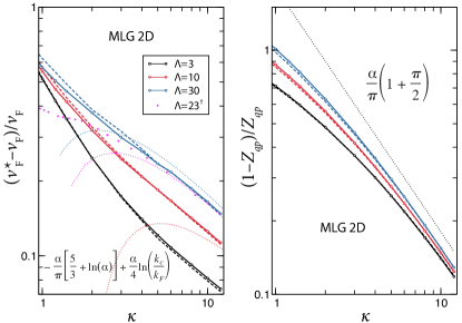
Figure 21: Renormalized Fermi velocity and the quasiparticle renormalization factor of the monolayer graphene for different values of the momentum cut-off $\Lambda=k_{c}/k_{\text{F}}$ as a function of dielectric constant. The log-log plots are compared with the scalings from Ref. Das Sarma et al. (2007) (dotted lines). ^† — data from Ref. Das Sarma and Hwang (2013).

Let us recapitulate first that we focus on the extrisic monolayer graphene system here, that is $k_{\text{F}}>0$. This is essentially a classical Fermi liquid in the marked contrast to the more complicated intrinsic graphene, $k_{\text{F}}=0$. For the latter, we refer to a comprehensive summary by Tang et al. Tang et al. (2018). While many conceptual problems do not arise in the extrinsic case, some important insight can be obtained from the intrinsic graphene. Consider for instance the expression for the Fermi velocity renormalization derived in Das Sarma et al. (2007) and plotted in Fig. 21 (left) as dotted lines

$$\frac{v_{\text{F}}^{*}-v_{\text{F}}}{v_{\text{F}}} =-\frac{\alpha}{\pi}\left(\frac{5}{3}+\log{\alpha}\right)+\frac{\alpha}{4}\log\left(\frac{k_{c}}{k_{\text{F}}}\right).$$ (97)

Here, the first part is extrinsic. It describes scattering processes in which the initial and the final state belong to the same band $s=s^{\prime}=1$ and contains no adjustable parameters. The second part is intrinsic, it includes scattering processes changing the band $s=-s^{\prime}=1$ and therefore depends on the momentum cut-off. In going to higher perturbative orders, such as including $\Sigma_{a\bar{a}}$, more and more processes involve interband scatterings and the role of intraband scattering is diminishing (as explicitly demonstrated for BLG, Fig. 17).

Let us inspect the qualitative dependence of the renormalized velocity on the interaction parameter $\alpha\simeq 2.2/\kappa$ (55). At higher $\alpha$, the dependence deviates from linear. This is already evident from the extrinsic part in Eq. (97). The intrinsic part shows a similar trend when computed beyond the leading order Tang et al. (2018). By consistently including other terms, one can improve the agreement of asymptotic theory with our numerical results.

Generally, it is believed that $G_{0}W_{0}$ result are already very accurate Das Sarma and Hwang (2013). However, higher-order diagrams have been treated in Ref. Barnes et al. (2014), quantum Monte-Carlo calculations were performed in Ref. Tang et al. (2018). All of them concern with intrinsic case, which is still relevant to some extent as stated above, however cannot be used for a direct comparison. They predict a slightly larger velocity renormalization, whereas, we observe here that the inclusion of $\Sigma_{a\bar{a}}$ leads to smaller values, Fig. 21.

Quasiparticle life-time

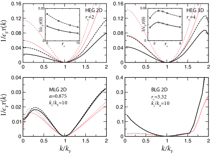
Figure 22: Inverse quasiparticle life-time (89) as a function of momentum. In the two insets, the values at the band bottom $\tau(k=0)^{-1}$ is shown for different $r_{s}$. Red lines additionally show the on-shell approximation (98) without (dashed) and with (full) $\Sigma_{a\bar{a}}$.

$1/\tau(k)$ is an essential ingredient of the quasiparticle spectral function (85). We determine it by solving the Dyson equation in the complex frequency plane. Also, it can be obtained from the Fermi Golden rule as advocated by Qian and Vignale Qian and Vignale (2005). From the discussion in Sec. II we know that the two are completely equivalent.

In Fig. 22 we summarize our finding for $\tau(k)$ computed for $0<k<2k_{\text{F}}$. In many studies, the “on-shell” imaginary self-energy is taken as a measure of the inverse life-time

$$\tau(k)^{-1} =-\operatorname{Im}\Sigma^{\text{R}}(k,\epsilon(k)),$$ (98)

where $\epsilon(k)$ is the bare dispersion relation. Apart from missing the $Z_{qp}$ prefactor, this approach is reasonable for $k\approx k_{\text{F}}$, where the difference between the “true” $\epsilon_{qp}(k)$ and the bare $\epsilon(k)$ spectrum is small. For $\xi_{k}=|\epsilon(k)-\epsilon_{\text{F}}|/\epsilon_{\text{F}}\gg 1$ the difference between Eq. (89) and the on-shell approximation (98) is substantial, as can be seen by comparing black and red lines in Fig. 22. We find, for instance for MLG, that the approximation incorrectly yields vanishing scattering rates at the Dirac point ($k=0$). One consequence of this is the diverging inelastic mean free path at zero temperature predicted in Ref. Li and Das Sarma (2013). On the other hand, Eq. (89) yields a finite value. It is worth noting that for the two HEG systems the correction upon the on-shell value is mostly associated with the quasiparticle strength $Z_{qp}$ renormalization, whereas, for graphene systems (MLG and BLG) the deviation of $\epsilon_{qp}(k)$ from $\epsilon(k)$ also plays a role.

Only for the two HEG systems the impact of $\Sigma_{a\bar{a}}$ is appreciable as depicted in the insets of Fig. 22 for $\tau(0)^{-1}$ for different $r_{s}$ values. The dependence is not always monotonic. For $\xi_{k}\ll 1$, we can compare with the asymptotic expressions from Ref. Giuliani and Vignale (2005)

$$\frac{1}{\tau(k)} =\frac{1}{4\pi}\zeta_{2}(r_{s})\xi_{k}^{2}\log\left(\frac{4}{\xi_{k}}\right), 2D;$$ (99)

$$\frac{1}{\tau(k)} =\frac{\pi}{8}\zeta_{3}(r_{s})\xi_{k}^{2}, 3D.$$ (100)

They have shown that the inclusion of exchange modifies the density-dependent prefactors $\zeta_{n}$ without affecting the functional form. However, the fitting of small values with this form is not a trivial task because of (i) numerical issues and (ii) our insufficient knowledge of the subleading terms. We follow Qian and Vignale Qian and Vignale (2005), where the coefficients $\zeta_{n}(r_{s})$ are derived:

$$\zeta_{2}(r_{s}) =\left[1+\frac{1}{2}\frac{\alpha_{2}^{2}r_{s}^{2}}{(1+\alpha_{2}r_{s})^{2}}\right]-\left[\frac{1}{4}+\frac{1}{2}\frac{\alpha_{2}r_{s}}{1+\alpha_{2}r_{s}}\right],$$ (101)

$$\zeta_{3}(r_{s}) =\frac{1}{2\lambda}\left[\tan^{-1}{\lambda}+\frac{\lambda}{1+\lambda^{2}}\right]$$

$$-\frac{1}{2\lambda}\left[\frac{1}{\sqrt{2+\lambda^{2}}}\cot^{-1}\frac{1}{\lambda\sqrt{2+\lambda^{2}}}\right],$$ (102)

with $\lambda=\pi^{1/2}/(\alpha_{3}r_{s})^{1/2}$. Here, the first brackets originate from the direct (d) processes and the second — from the exchange (ex). In Fig. 23, we determine the ratio of exchange to direct scattering rates using the on-shell approximation (98) with $\Sigma_{a\bar{a}}$ and $\Sigma_{G_{0}W_{0}}$, respectively. In 3D, the agreement with the analytical results (99) is very good, whereas, in 2D we find that the ratio is smaller. One possible explanation of this discrepancy could be the absence of the plasmonic contributions to the direct scattering in Ref. Qian and Vignale (2005).

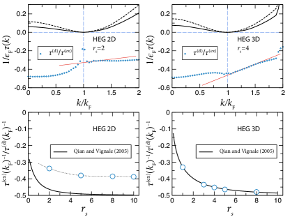
Figure 23: Top row: determination of the ratio $\tau^{\text{(ex)}}(k)^{-1}/\tau^{\text{(d)}}(k)^{-1}$ for the homogeneous electron gas in 2D and 3D illustrating numerical difficulties of taking the $k\rightarrow k_{\text{F}}$ limit. Bottom row: comparison with analytical results of Ref. Qian and Vignale (2005): $\zeta_{n}^{\text{(ex)}}(r_{s})/\zeta_{n}^{\text{(d)}}(r_{s})$, see Eq. (101,102).

Besides ratios, we also compared absolute values with analytical predictions and found systematic underestimates. However, this should not be a surprise because the theory only yields the leading terms.

For MLG, the inverse life-time follows the same asymptotic with famous logarithmic correction Giuliani and Quinn (1982) as for HEG 2D, Eq. (99) Li and Das Sarma (2013). Polini and Vignale provided a very pedagogical derivation of this fact Polini and Vignale (2014), however, exchange contributions were not included. Our simulations show that they are indeed small for MLG and BLG systems, Fig. 22. One interesting conclusion of Ref. Polini and Vignale (2014) is that the scatterings are dominated by the “collinear scattering singularity”, that is, the momenta of electrons involved in the scattering are mostly parallel to each other. We find it interesting because of its apparent similarities with the scattering processes shaping $\Sigma_{2x}$, see our analysis in Sec. V.2. Another interesting conclusion of the analytical formula is that the life-time is independent of the dielectric constant. While our numerics shows that its only approximately true for full-fledged calculations using Eq. (89), an illustration on why this is the case for the on-shell $\tau^{-1}$ is provided in Fig. 24. There, we plot the imaginary self-energy part for $k=1.6k_{\text{F}}$ and three different dielectric constants, $\kappa=0.5,\,1.0,\,2.5$ resolving plasmonic and $p$-$h$ contributions. Approaching the “on-shell” frequency marked as a vertical dashed line, the curves essentially fall on top of each other. The figure also illustrates the difficulties of the numerical determination of the asymptotic prefactors in Eq. (99) (for MLG they also depend on the momentum cut-off).

Figure 24: Imaginary self-energy part of MLG for different interaction strengths. The on-shell value is only weakly dependent on $\kappa$ in agreement with the analytical result of Polini and Vignale Polini and Vignale (2014).

VI Conclusions

Hedin’s set of functional equations allows us to expand the electron self-energy in terms of dressed $G$ and $W$. The first term of such an expansion — the $GW$ approximation — has been successfully applied to many systems. However, there are cases when this approximation is insufficient and higher-order terms need to be taken into account. One such approximation has been derived in our previous work starting from the first- and second-order SE Stefanucci et al. (2014). $\Sigma_{aa}+[\Sigma_{cc}+\Sigma_{c\bar{c}}]+\Sigma_{a\bar{a}}$ describes three distinct scattering processes in many-body systems, comprises all the first- and second-order terms and a subset of third and fourth order terms, and, crucially, has the PSD property Pavlyukh et al. (2016). In this work focused on $\Sigma_{a\bar{a}}$, relevant for small energy transfers, and evaluated it in the quasiparticle approximation for the electron GF and RPA for the screened interaction. We found that screening is important and must be determined consistently. For inconsistent screening, unphysical singularities have been observed in $\Sigma_{2x}$, which is the bare Coulomb limit of $\Sigma_{a\bar{a}}$. Nonetheless, $\Sigma_{2x}$ provides important corrections to the total energy in full agreement with analytic results of Onsager et al. Onsager et al. (1966).

We conducted a comprehensive investigation of the impact of $\Sigma_{a\bar{a}}$ on quasiparticle properties of the homogeneous electron gas in 2D and 3D, and of the mono- and bilayer graphene. The quasiparticle renormalization factor $Z_{qp}(k_{\text{F}})$, the effective mass $m^{*}$, the Fermi velocity $v_{\text{F}}^{*}$, and the quasiparticle life-time $\tau(k)$ have been computed for a range of interaction strengths controlled by the density $r_{s}$ or the dielectric function $\kappa$. In the weakly correlated limit ($r_{s}\ll 1$ or $\kappa\gg 1$), we compared with asymptotic expansions, and in the correlated regime with results of other theories such as quantum Monte Carlo and perturbative calculations including local field factors.

It is known that exchange processes encoded in $\Sigma_{a\bar{a}}$ reduce the quasiparticle scattering rate. This has been shown in the asymptotic limit $\omega\rightarrow\infty$ by Vogt et al. Vogt et al. (2004) and in the vicinity of $k_{\text{F}}$ by Qian and Vignale Qian and Vignale (2005). Besides confirming this finding using a completely different methodology, we also observed an appreciable effect of $\Sigma_{a\bar{a}}$ on the effective mass $m^{*}$ and quasiparticle strength $Z_{qp}$ in 3D HEG. The effect is smaller in 2D, especially for graphene systems, as anticipated.

Although we have focused on one particular scattering process the PSD diagrammatic construction is versatile and applicable to realistic multiband systems. Furthermore, the PSD diagrams remain PSD upon replacement of the zero-temperature Green’s function with the finite-temperature Kas and Rehr (2017) or any excited-state Green’s function. This latter possibility opens the way toward the systematic inclusion of vertex corrections in the spectral function of systems in a (quasi) steady-state. Investigations in the field of, e.g., molecular transport and time-resolved (tr) and angle-resolved photoemission spectroscopy (ARPES) are therefore foreseeable in the near future. The spectral function is indeed a key quantity to determine the conductance of atomic-scale junctions, and MBPT calculations have so far been limited to the $GW$ Thygesen and Rubio (2007); Spataru et al. (2009); Neaton et al. (2006); Myöhänen et al. (2008, 2009) and second-Born Myöhänen et al. (2008, 2009) approximation. Similarly, the tr-ARPES signal is related to the transient spectral function Freericks et al. (2009); Perfetto et al. (2016) which in semiconductor or insulators can be evaluated using a steady-state approximation (provided that the carrier relaxation time is much longer than the probe pulse). In this context Hyrkäs et al. (2019) the PSD diagrammatic construction may provide a powerful tool in the field of light-induced exciton fluids, whose incoherent plasma phase Semkat et al. (2009); Perfetto et al. (2016); Steinhoff et al. (2017) and coherent condensed phase Rustagi and Kemper (2018, 2019); Perfetto et al. (2019); Christiansen et al. (2019); Perfetto et al. (2020); Hanai et al. (2016); Becker et al. (2019) are currently under intense investigations.

Appendix A Hilbert transform and spectral functions

Hilbert transform is an important part of our numerical procedure. We define

$$H\left[x\right](t) =\frac{1}{\pi}\mathcal{P}\int_{-\infty}^{\infty}\!\!\mathrm{d}\tau\,\frac{x(\tau)}{t-\tau}.$$ (103)

It has the properties $H\left[H[x]\right](t)=-x(t)$, $H^{-1}\left[x\right](t)=-H\left[x\right](t)$, and is computed using FFT. In particular we need the relation between the real part of the correlation self-energy and the rate function $\Gamma(k,\omega)$, Eq. (1), which in our approach is computed by the Monte-Carlo method,

$$\operatorname{Re}\Sigma^{\text{R}}_{c}(k,\omega) =\tfrac{1}{2}H[\Gamma(k)](\omega),$$ (104)

$$\tfrac{1}{2}\Gamma(k,\omega) =-\operatorname{Im}\Sigma^{\text{R}}_{c}(k,\omega).$$ (105)

There are following possibilities to obtain positive spectral functions starting from the second-order self-energy:

$$\mp i\Sigma_{aa}^{\lessgtr}(k,\omega) \geq 0,$$ (106a)

$$\mp i\left(\Sigma_{cc}^{\lessgtr}+\Sigma_{c\bar{c}}^{\lessgtr}\right)(k,\omega) \geq 0,$$ (106b)

$$\mp i\left(\Sigma_{aa}^{\lessgtr}+\Sigma_{a\bar{a}}^{\lessgtr}\right)(k,\omega) \geq 0.$$ (106c)

Consequently, the sum of all contributions given by Eq. (8) is also PSD. By using the method from our earlier work Stefanucci et al. (2014), these results can also be generalized to any dressed GFs that possess a positive spectral function.

Appendix B Equilibrium propagators

We define the bare electron propagators as averages of the field operators in the Heisenberg picture over the non-interacting state

$$g^{<}(1,2) =i\langle\hat{\psi}_{H}^{\dagger}(2)\hat{\psi}_{H}(1)\rangle_{0}, g^{>}(1,2) =-i\langle\hat{\psi}_{H}(1)\hat{\psi}_{H}^{\dagger}(2)\rangle_{0},$$

fulfilling the symmetry relations

$$ig^{\lessgtr}(1,2) =\left(ig^{\lessgtr}(2,1)\right)^{*}.$$ (107)

Analogically, the density-density correlators are defined with respect to the interacting ground state

$$\chi^{>}(1,2) =-i\langle\Delta\hat{n}_{H}(1)\Delta\hat{n}_{H}(2)\rangle,$$

$$\chi^{<}(1,2) =-i\langle\Delta\hat{n}_{H}(2)\Delta\hat{n}_{H}(1)\rangle,$$

with the density deviation $\Delta\hat{n}_{H}(1)=\hat{n}_{H}(1)-\langle\hat{n}_{H}(1)\rangle$. They fulfill the symmetries

$$i\chi^{\lessgtr}(1,2) =\left(i\chi^{\lessgtr}(2,1)\right)^{*}.$$ (108)

Because the screened interaction is directly related to $\chi$

$$W(1,2) =v(1,2)+\iint\mathrm{d}(3,4)\,v(1,3)\chi(3,4)v(4,3),$$ (109)

all the symmetry and analytic properties also hold for $W$.

For homogeneous systems the momentum-energy representation is useful, which we formulate here in Fermi units ($k_{\text{F}}$, $\epsilon_{\text{F}}$). The Kubo-Martin-Schwinger conditions allow us to write the lesser/greater propagators in terms of the retarded ones,

$$g^{<}(x,\zeta) =-2in_{\text{F}}(\zeta)\operatorname{Im}g^{\text{R}}(x,\zeta),$$ (110a)

$$g^{>}(x,\zeta) =-2i(n_{\text{F}}(\zeta)-1)\operatorname{Im}g^{\text{R}}(x,\zeta);$$ (110b)

$$W_{0}^{<}(y,\xi) =+2in_{\text{B}}(\xi)\operatorname{Im}W_{0}^{\text{R}}(y,\xi),$$ (110c)

$$W_{0}^{>}(y,\xi) =+2i(n_{\text{B}}(\xi)+1)\operatorname{Im}W_{0}^{\text{R}}(y,\xi).$$ (110d)

$n_{\text{F/B}}$ are the Fermi/Bose distribution functions, which at zero temperature reduce to simple step-functions

$$n_{\text{F}}(\zeta) =\theta(1-\zeta), \bar{n}_{\text{F}}(\zeta)=1-n_{\text{F}}(\zeta);$$ (111a)

$$n_{\text{B}}(\xi) =-\theta(-\xi)=\theta(\xi)-1, n_{\text{B}}(\xi)+1=\theta(\xi).$$ (111b)

For the bare propagators we furthermore have

$$g^{\text{R}}(x,\zeta) =\frac{1}{\zeta-\epsilon(x)+i\eta},$$ (112)

and we use a spectral representation of the screened interaction

$$W_{0}^{\text{R}}(y,\xi) =v(y)+\int_{0}^{\infty}\!\mathrm{d}\omega\frac{2\omega\,C(y,\xi)}{(\xi+i\eta)^{2}-\omega^{2}},$$ (113)

where $v(y)$ is the bare Coulomb interaction. It fulfills the symmetry property

$$\left[W_{0}^{\text{R}}(y,\xi)\right]^{*} =W_{0}^{\text{R}}(y,-\xi).$$ (114)

Comparing it with the Hilbert transform of the inverse dielectric function

$$\frac{1}{\varepsilon^{\text{R}}(y,\xi)} =1-\int_{0}^{\infty}\!\frac{\mathrm{d}\omega}{\pi}\operatorname{Im}\left[\frac{1}{\varepsilon^{\text{R}}(y,\omega)}\right]\frac{2\omega}{(\xi+i\eta)^{2}-\omega^{2}},$$ (115)

we have for the spectral function of continuous spectrum

$$C(y,\omega) =v(y)\operatorname{Im}\left[-\frac{1}{\pi}\frac{1}{\varepsilon^{\text{R}}(y,\omega)}\right],$$ (116)

and for plasmons $C(y,\omega)=C(y)\delta\left(\omega-\Omega(y)\right)$ with

$$C(y) =v(y)\left[\left.\frac{\partial\operatorname{Re}\varepsilon^{\text{R}}(y,\xi)}{\partial\xi}\right|_{\xi=\Omega(y)}\right]^{-1}.$$ (117)

The time-ordered ($W_{0}^{\text{T}}\equiv W_{0}^{--}$) and the anti-time-ordered ($W_{0}^{\overline{\text{T}}}\equiv W_{0}^{++}$ ) screened interactions read

$$W_{0}^{\text{T}}(y,\xi) =v(y)+\int_{0}^{\infty}\!\mathrm{d}\omega\frac{2\omega\,C(y,\omega)}{\xi^{2}-(\omega-i\eta)^{2}},$$ (118)

$$W_{0}^{\overline{\text{T}}}(y,\xi) =-\left[W_{0}^{\text{T}}(y,\xi)\right]^{*},$$ (119)

with $W_{0}^{\text{T}}(y,-\xi)=W_{0}^{\text{T}}(y,\xi)$.

Appendix C Polarizability of MLG

The dynamical polarization of graphene at finite doping has been computed by Hwang and Das Sarma Hwang and Das Sarma (2007) and by Wunsch et al. Wunsch et al. (2006). We present here for completeness the functions $G_{r}$,

$$G_{r}(y,\xi) =\begin{dcases*}0&1A\\ \pi+G_{<}(z_{1})&2A\\ \pi+G_{<}(z_{1})+G_{<}(z_{2})&3A\\ -G_{>}(z_{2})+G_{>}(-z_{1})&1B\\ -G_{>}(z_{2})&2B\\ -G_{>}(z_{2})+G_{>}(z_{1})&3B\end{dcases*},$$ (120)

and $G_{i}$,

$$G_{i}(y,\xi) =\begin{dcases*}G_{>}(z_{2})-G_{>}(-z_{1})&1A\\ G_{>}(z_{2})&2A\\ 0&3A\\ 0&1B\\ \pi+G_{<}(z_{1})&2B\\ \pi&3B\end{dcases*}.$$ (121)

that define the dielectric function in Eqs. (56,58) with

$$z_{1} =\frac{\xi-2}{y}, z_{2} =\frac{\xi+2}{y},$$ (122)

and

$$G_{>}(z) =z\sqrt{z^{2}-1}-\mathrm{arccosh}(z),$$ (123)

$$G_{<}(z) =z\sqrt{1-z^{2}}-\arccos(z).$$ (124)

Notice that A-domains are for $\xi<y$ and $B$-domains are for $\xi>y$ as shown in Fig. 5.

Appendix D Polarizability of BLG

We start by defining the four critical lines

$$r_{1} =y^{2}+2y+\xi+2; r_{2} =y^{2}+\xi;$$

$$r_{3} =y^{2}-2y+\xi+2; r_{4} =\frac{y^{2}}{2}+\xi.$$

Furthermore, we introduce some auxiliary functions:

$$q_{1} =\frac{y^{2}-2\xi}{4\xi}\log 2+\frac{r_{4}}{2\xi}\log|r_{4}|-\frac{r_{2}}{2\xi}\log|r_{2}|\operatorname{\theta}(y-1)$$

$$\qquad+\left(\frac{r_{2}}{4\xi}\log|1+\xi|+\frac{y^{2}}{4\xi}\log|y^{2}|\right)\mathrm{sign}(y-1),$$ (125)

$$q_{2} =\left[\frac{|r_{2}|}{4\xi}\log\left|\frac{(2+\xi)\sqrt{r_{2}r_{2}}+\xi\sqrt{r_{1}r_{3}}}{(2+\xi)\sqrt{r_{2}r_{2}}-\xi\sqrt{r_{1}r_{3}}}\right|\right.$$

$$\quad\left.-\frac{1}{4}\log\left|\frac{\sqrt{r_{1}r_{3}}+2+\xi}{\sqrt{r_{1}r_{3}}-(2+\xi)}\right|\right]\left(\operatorname{\theta}(-r_{1})-\operatorname{\theta}(r_{3})\right),$$ (126)

$$p_{1} =\left[\frac{r_{2}}{2\xi}\arctan\left(\frac{(2+\xi)r_{2}}{\xi\sqrt{-r_{1}r_{3}}}\right)\right.$$

$$\qquad\left.+\frac{1}{2}\arccos\left(\frac{2+\xi}{y\sqrt{-2r_{4}}}\right)\right]\operatorname{\theta}(-r_{1}r_{3}),$$ (127)

$$p_{2} =\frac{\pi r_{2}}{4\xi}\mathrm{sign}(r_{2})\operatorname{\theta}(-r_{1}r_{3})+\frac{\pi r_{4}}{\xi}\operatorname{\theta}(y-2)\operatorname{\theta}(-r_{4})\operatorname{\theta}(r_{3})$$

$$\qquad-\frac{\pi y^{2}}{2\xi}\operatorname{\theta}(-r_{1}).$$ (128)

With the help of these definitions

$$\operatorname{Re}\Pi_{2}(y,\xi) =q_{1}+q_{2}; \operatorname{Im}\Pi_{2}(y,\xi) =p_{1}+p_{2}.$$ (129)

Appendix E Solution of the Dyson equation

Let us recapitulate possible approaches to the solution of the Dyson equation

$$G(k,\omega) =g(k,\omega)+g(k,\omega)\Sigma(k,\omega)G(k,\omega)$$ (130)

following Ref. Stefanucci and van Leeuwen (2013). In the preceding sections the self-energy is computed using bare propagators (110), $\Sigma=\Sigma[g,W_{0}]$. This approach has an inherent problem that the $k=k_{\text{F}}$ state is no longer a sharp quasiparticle state. We still can improve the one-shot calculations by applying some rigid shift $\Delta\mu$ to all poles,

$$G_{0}(k,\omega) =\frac{1}{\omega-\epsilon_{0}(k)-\Delta\mu+i\eta}=g(k,\omega-\Delta\mu).$$ (131)

The respective self-energy then reads

$$\Sigma[G_{0},W_{0}](k,\omega) =\Sigma[g,W_{0}](k,\omega-\Delta\mu),$$ (132)

allowing to rewrite the quasiparticle approximation for the Dyson’s equation

$$\epsilon(k) =\epsilon_{0}(k)+\Sigma[g,W_{0}](k,\epsilon(k)-\Delta\mu),$$ (133)

$$\tilde{\epsilon}(k) =\epsilon_{0}(k)-\Delta\mu+\Sigma[g,W_{0}](k,\tilde{\epsilon}(k)),$$ (134)

Thus, the quasiparticle approximation for $G$ reads

$$G(k,\omega) =\frac{1}{\omega-\tilde{\epsilon}(k)}.$$ (135)

Now we demand that the solution of the Dyson equation at $k=k_{\text{F}}$ takes the form

$$G(k_{\text{F}},\omega) =\frac{1}{\omega-\mu+i\eta}=G_{0}(k_{\text{F}},\omega).$$ (136)

and coincides with the improved propagator $G_{0}$ (131) representing a sharp quasiparticle peak at the chemical potential. The consistency condition (136) provides the interpretation of $\Delta\mu$ as the correlation shift of the chemical potential

$$\Delta\mu =\mu-\epsilon_{\text{F}},$$ (137)

and allows to determine it. To this end, we insert Eq. (136) into Eq. (133) leading to

$$\mu =\epsilon_{\text{F}}+\operatorname{Re}\Sigma[G_{0},W_{0}](k_{\text{F}},\mu).$$ (138)

This point and the connection of $\mu$ to the total energy per electron is explained in Ref. Hedin and Lundqvist (1970) (p. 82). Combining Eq. (137) with Eq. (138) we obtain

$$\Delta\mu =\operatorname{Re}\Sigma[g,W_{0}](k_{\text{F}},\epsilon_{\text{F}}).$$ (139)

Thus, $\Delta\mu$ is expressed solely in terms of the self-energy for $k=k_{\text{F}}$ and $\omega=\epsilon_{\text{F}}$. In the case of MLG and BLG having two bands, one additionally sets the band index $s$ consistent with the doping (typically the chemical potential is above the Dirac point implying $s=+1$).

References

• Hedin (1965) L. Hedin, Phys. Rev. 139, A796 (1965).
• Minnhagen (1974) P. Minnhagen, J. Phys. C 7, 3013 (1974).
• Minnhagen (1975) P. Minnhagen, J. Phys. C 8, 1535 (1975).
• Stefanucci et al. (2014) G. Stefanucci, Y. Pavlyukh, A.-M. Uimonen,  and R. van Leeuwen, Phys. Rev. B 90, 115134 (2014).
• Uimonen et al. (2015) A.-M. Uimonen, G. Stefanucci, Y. Pavlyukh,  and R. van Leeuwen, Phys. Rev. B 91, 115104 (2015).
• Pavlyukh et al. (2016) Y. Pavlyukh, A.-M. Uimonen, G. Stefanucci,  and R. van Leeuwen, Phys. Rev. Lett. 117, 206402 (2016).
• Holm and von Barth (1998) B. Holm and U. von Barth, Phys. Rev. B 57, 2108 (1998).
• Riley et al. (2018) J. M. Riley, F. Caruso, C. Verdi, L. B. Duffy, M. D. Watson, L. Bawden, K. Volckaert, G. van der Laan, T. Hesjedal, M. Hoesch, F. Giustino,  and P. D. C. King, Nat. Commun. 9, 2305 (2018).
• Holm and Aryasetiawan (1997) B. Holm and F. Aryasetiawan, Phys. Rev. B 56, 12825 (1997).
• Guzzo et al. (2014) M. Guzzo, J. J. Kas, L. Sponza, C. Giorgetti, F. Sottile, D. Pierucci, M. G. Silly, F. Sirotti, J. J. Rehr,  and L. Reining, Phys. Rev. B 89, 085425 (2014).
• Langreth (1970) D. C. Langreth, Phys. Rev. B 1, 471 (1970).
• Pavlyukh (2017) Y. Pavlyukh, Sci. Rep. 7, 504 (2017).
• Balzer et al. (2010) K. Balzer, S. Bauch,  and M. Bonitz, Phys. Rev. A 82, 033427 (2010).
• Perfetto et al. (2015) E. Perfetto, A.-M. Uimonen, R. van Leeuwen,  and G. Stefanucci, Phys. Rev. A 92, 033419 (2015).
• Schüler and Pavlyukh (2018) M. Schüler and Y. Pavlyukh, Phys. Rev. B 97, 115164 (2018).
• Ziesche (2007) P. Ziesche, Ann. Phys. 16, 45 (2007).
• Qian and Vignale (2005) Z. Qian and G. Vignale, Phys. Rev. B 71, 075112 (2005).
• Almbladh (2006) C.-O. Almbladh, J. Phys. Conf. Ser. 35, 127 (2006).
• Pavlyukh et al. (2015) Y. Pavlyukh, M. Schüler,  and J. Berakdar, Phys. Rev. B 91, 155116 (2015).
• Schüler et al. (2016) M. Schüler, Y. Pavlyukh, P. Bolognesi, L. Avaldi,  and J. Berakdar, Sci. Rep. 6, 24396 (2016).
• Grüneis et al. (2009) A. Grüneis, M. Marsman, J. Harl, L. Schimka,  and G. Kresse, J. Chem. Phys. 131, 154115 (2009).
• Ren et al. (2015) X. Ren, N. Marom, F. Caruso, M. Scheffler,  and P. Rinke, Phys. Rev. B 92, 081104(R) (2015).
• Lundqvist (1968) B. I. Lundqvist, Phys. Kondens. Mater. 7, 117 (1968).
• Santoro and Giuliani (1989) G. E. Santoro and G. F. Giuliani, Phys. Rev. B 39, 12818 (1989).
• Hwang and Das Sarma (2008a) E. H. Hwang and S. Das Sarma, Phys. Rev. B 77, 081412(R) (2008a).
• Polini et al. (2008) M. Polini, R. Asgari, G. Borghi, Y. Barlas, T. Pereg-Barnea,  and A. H. MacDonald, Phys. Rev. B 77, 081411(R) (2008).
• Sensarma et al. (2011) R. Sensarma, E. H. Hwang,  and S. Das Sarma, Phys. Rev. B 84, 041408(R) (2011).
• Kotov et al. (2012) V. N. Kotov, B. Uchoa, V. M. Pereira, F. Guinea,  and A. H. Castro Neto, Rev. Mod. Phys. 84, 1067 (2012).
• Pavlyukh et al. (2013) Y. Pavlyukh, A. Rubio,  and J. Berakdar, Phys. Rev. B 87, 205124 (2013).
• Stefanucci and van Leeuwen (2013) G. Stefanucci and R. van Leeuwen, Nonequilibrium Many-Body Theory of Quantum Systems: A Modern Introduction (Cambridge University Press, Cambridge, 2013).
• Strinati (1988) G. Strinati, Riv. Nuovo Cimento 11, 1 (1988).
• van Leeuwen and Stefanucci (2012) R. van Leeuwen and G. Stefanucci, Phys. Rev. B 85, 115119 (2012).
• Freeman (1977) D. L. Freeman, Phys. Rev. B 15, 5512 (1977).
• Das Sarma et al. (2011) S. Das Sarma, S. Adam, E. H. Hwang,  and E. Rossi, Rev. Mod. Phys. 83, 407 (2011).
• Basov et al. (2016) D. N. Basov, M. M. Fogler,  and F. J. Garcia de Abajo, Science 354, aag1992 (2016).
• Czachor et al. (1982) A. Czachor, A. Holas, S. R. Sharma,  and K. S. Singwi, Phys. Rev. B 25, 2144 (1982).
• Stern (1967) F. Stern, Phys. Rev. Lett. 18, 546 (1967).
• Giuliani and Vignale (2005) G. Giuliani and G. Vignale, Quantum theory of the electron liquid (Cambridge University Press, Cambridge, UK, 2005).
• Gradshteyn and Ryzhik (2007) I. S. Gradshteyn and I. M. Ryzhik, Table of integrals, series, and products, 7th ed. (Elsevier, Amsterdam, 2007).
• Ando (2006) T. Ando, J. Phys. Soc. Jpn. 75, 074716 (2006).
• Basov et al. (2014) D. N. Basov, M. M. Fogler, A. Lanzara, F. Wang,  and Y. Zhang, Rev. Mod. Phys. 86, 959 (2014).
• Hwang and Das Sarma (2007) E. H. Hwang and S. Das Sarma, Phys. Rev. B 75, 205418 (2007).
• Wunsch et al. (2006) B. Wunsch, T. Stauber, F. Sols,  and F. Guinea, New J. Phys. 8, 318 (2006).
• Hwang et al. (2018) E. H. Hwang, R. E. Throckmorton,  and S. Das Sarma, Phys. Rev. B 98, 195140 (2018).
• Trevisanutto et al. (2008) P. E. Trevisanutto, C. Giorgetti, L. Reining, M. Ladisa,  and V. Olevano, Phys. Rev. Lett. 101, 226405 (2008).
• Hwang et al. (2007) E. H. Hwang, B. Y.-K. Hu,  and S. Das Sarma, Phys. Rev. Lett. 99, 226801 (2007).
• Sensarma et al. (2010) R. Sensarma, E. H. Hwang,  and S. Das Sarma, Phys. Rev. B 82, 195428 (2010).
• Hwang and Das Sarma (2008b) E. H. Hwang and S. Das Sarma, Phys. Rev. Lett. 101, 156802 (2008b).
• von Barth and Holm (1996) U. von Barth and B. Holm, Phys. Rev. B 54, 8411 (1996).
• Giuliani and Quinn (1982) G. F. Giuliani and J. J. Quinn, Phys. Rev. B 26, 4421 (1982).
• Zhang and Das Sarma (2005) Y. Zhang and S. Das Sarma, Phys. Rev. B 71, 045322 (2005).
• Lischner et al. (2014) J. Lischner, D. Vigil-Fowler,  and S. G. Louie, Phys. Rev. B 89, 125430 (2014).
• Bostwick et al. (2010) A. Bostwick, F. Speck, T. Seyller, K. Horn, M. Polini, R. Asgari, A. H. MacDonald,  and E. Rotenberg, Science 328, 999 (2010).
• Walter et al. (2011) A. L. Walter, A. Bostwick, K.-J. Jeon, F. Speck, M. Ostler, T. Seyller, L. Moreschini, Y. J. Chang, M. Polini, R. Asgari, A. H. MacDonald, K. Horn,  and E. Rotenberg, Phys. Rev. B 84, 085410 (2011).
• Carbotte et al. (2012) J. P. Carbotte, J. P. F. LeBlanc,  and E. J. Nicol, Phys. Rev. B 85, 201411(R) (2012).
• Das Sarma and Hwang (2013) S. Das Sarma and E. H. Hwang, Phys. Rev. B 87, 045425 (2013).
• Sabashvili et al. (2013) A. Sabashvili, S. Östlund,  and M. Granath, Phys. Rev. B 88, 085439 (2013).
• Glasser and Lamb (2007) M. L. Glasser and G. Lamb, J. Phys. A 40, 1215 (2007).
• Onsager et al. (1966) L. Onsager, L. Mittag,  and M. J. Stephen, Ann. Phys. 473, 71 (1966).
• Isihara and Ioriatti (1980) A. Isihara and L. Ioriatti, Phys. Rev. B 22, 214 (1980).
• Glasser (2018) M. L. Glasser, in Many-body Approaches at Different Scales, edited by G. Angilella and C. Amovilli (Springer International Publishing, Cham, 2018) pp. 291–296.
• Vogt et al. (2004) M. Vogt, R. Zimmermann,  and R. J. Needs, Phys. Rev. B 69, 045113 (2004).
• González et al. (1999) J. González, F. Guinea,  and M. A. H. Vozmediano, Phys. Rev. B 59, R2474 (1999).
• Barnes et al. (2014) E. Barnes, E. H. Hwang, R. E. Throckmorton,  and S. Das Sarma, Phys. Rev. B 89, 235431 (2014).
• Chubukov (1993) A. V. Chubukov, Phys. Rev. B 48, 1097 (1993).
• Holzmann et al. (2009) M. Holzmann, B. Bernu, V. Olevano, R. M. Martin,  and D. M. Ceperley, Phys. Rev. B 79, 041308(R) (2009).
• Holzmann et al. (2011) M. Holzmann, B. Bernu, C. Pierleoni, J. McMinis, D. M. Ceperley, V. Olevano,  and L. Delle Site, Phys. Rev. Lett. 107, 110402 (2011).
• Asgari et al. (2005) R. Asgari, B. Davoudi, M. Polini, G. F. Giuliani, M. P. Tosi,  and G. Vignale, Phys. Rev. B 71, 045323 (2005).
• Simion and Giuliani (2008) G. E. Simion and G. F. Giuliani, Phys. Rev. B 77, 035131 (2008).
• Kukkonen and Overhauser (1979) C. A. Kukkonen and A. W. Overhauser, Phys. Rev. B 20, 550 (1979).
• Kutepov and Kotliar (2017) A. L. Kutepov and G. Kotliar, Phys. Rev. B 96, 035108 (2017).
• Sensarma et al. (2012) R. Sensarma, E. H. Hwang,  and S. Das Sarma, Phys. Rev. B 86, 079912(E) (2012).
• Daniel and Vosko (1960) E. Daniel and S. H. Vosko, Phys. Rev. 120, 2041 (1960).
• Galitski and Das Sarma (2004) V. M. Galitski and S. Das Sarma, Phys. Rev. B 70, 035111 (2004).
• Drummond and Needs (2009) N. D. Drummond and R. J. Needs, Phys. Rev. B 80, 245104 (2009).
• Gell-Mann (1957) M. Gell-Mann, Phys. Rev. 106, 369 (1957).
• Mahan (2000) G. Mahan, Many-particle physics, 3rd ed. (Kluwer Academic/Plenum Publishers, New York, 2000).
• Janak (1969) J. F. Janak, Phys. Rev. 178, 1416 (1969).
• Ting et al. (1975) C. S. Ting, T. K. Lee,  and J. J. Quinn, Phys. Rev. Lett. 34, 870 (1975).
• Ando et al. (1982) T. Ando, A. B. Fowler,  and F. Stern, Rev. Mod. Phys. 54, 437 (1982).
• Saraga and Loss (2005) D. S. Saraga and D. Loss, Phys. Rev. B 72, 195319 (2005).
• Eich et al. (2017) F. G. Eich, M. Holzmann,  and G. Vignale, Phys. Rev. B 96, 035132 (2017).
• Das Sarma et al. (2007) S. Das Sarma, E. H. Hwang,  and W.-K. Tse, Phys. Rev. B 75, 121406(R) (2007).
• Tang et al. (2018) H.-K. Tang, J. N. Leaw, J. N. B. Rodrigues, I. F. Herbut, P. Sengupta, F. F. Assaad,  and S. Adam, Science 361, 570 (2018).
• Li and Das Sarma (2013) Q. Li and S. Das Sarma, Phys. Rev. B 87, 085406 (2013).
• Zheng and Das Sarma (1996) L. Zheng and S. Das Sarma, Phys. Rev. B 53, 9964 (1996).
• Reizer and Wilkins (1997) M. Reizer and J. W. Wilkins, Phys. Rev. B 55, R7363 (1997).
• Polini and Vignale (2014) M. Polini and G. Vignale, arXiv:1404.5728 [cond-mat]  (2014).
• Kas and Rehr (2017) J. J. Kas and J. J. Rehr, Phys. Rev. Lett. 119, 176403 (2017).
• Thygesen and Rubio (2007) K. S. Thygesen and A. Rubio, J. Chem. Phys. 126, 091101 (2007).
• Spataru et al. (2009) C. D. Spataru, M. S. Hybertsen, S. G. Louie,  and A. J. Millis, Phys. Rev. B 79, 155110 (2009).
• Neaton et al. (2006) J. B. Neaton, M. S. Hybertsen,  and S. G. Louie, Phys. Rev. Lett. 97, 216405 (2006).
• Myöhänen et al. (2008) P. Myöhänen, A. Stan, G. Stefanucci,  and R. van Leeuwen, Eurphys. Lett. 84, 67001 (2008).
• Myöhänen et al. (2009) P. Myöhänen, A. Stan, G. Stefanucci,  and R. van Leeuwen, Phys. Rev. B 80, 115107 (2009).
• Freericks et al. (2009) J. K. Freericks, H. R. Krishnamurthy,  and T. Pruschke, Phys. Rev. Lett. 102, 136401 (2009).
• Perfetto et al. (2016) E. Perfetto, D. Sangalli, A. Marini,  and G. Stefanucci, Phys. Rev. B 94, 245303 (2016).
• Hyrkäs et al. (2019) M. Hyrkäs, D. Karlsson,  and R. van Leeuwen, Phys. Status Solidi B 256, 1800615 (2019).
• Semkat et al. (2009) D. Semkat, F. Richter, D. Kremp, G. Manzke, W.-D. Kraeft,  and K. Henneberger, Phys. Rev. B 80, 155201 (2009).
• Steinhoff et al. (2017) A. Steinhoff, M. Florian, M. Rösner, G. Schönhoff, T. O. Wehling,  and F. Jahnke, Nat. Commun. 8, 1166 (2017).
• Rustagi and Kemper (2018) A. Rustagi and A. F. Kemper, Phys. Rev. B 97, 235310 (2018).
• Rustagi and Kemper (2019) A. Rustagi and A. F. Kemper, Phys. Rev. B 99, 125303 (2019).
• Perfetto et al. (2019) E. Perfetto, D. Sangalli, A. Marini,  and G. Stefanucci, Phys. Rev. Materials 3, 124601 (2019).
• Christiansen et al. (2019) D. Christiansen, M. Selig, E. Malic, R. Ernstorfer,  and A. Knorr, Phys. Rev. B 100, 205401 (2019).
• Perfetto et al. (2020) E. Perfetto, S. Bianchi,  and G. Stefanucci, Phys. Rev. B 101, 041201(R) (2020).
• Hanai et al. (2016) R. Hanai, P. B. Littlewood,  and Y. Ohashi, J. Low Temp. Phys. 183, 127 (2016).
• Becker et al. (2019) K. W. Becker, H. Fehske,  and V.-N. Phan, Phys. Rev. B 99, 035304 (2019).
• Hedin and Lundqvist (1970) L. Hedin and S. Lundqvist, in Solid State Physics, Vol. 23, edited by D. T. a. H. E. Frederick Seitz (Academic Press, New York, 1970) pp. 1–181.