High-order well-balanced finite volume schemes for hydrodynamic equations with nonlocal free energy
Abstract.
We propose high-order well-balanced finite-volume schemes for a broad class of hydrodynamic systems with attractive-repulsive interaction forces and linear and nonlinear damping. Our schemes are suitable for free energies containing convolutions of an interaction potential with the density, which are essential for applications such as the Keller-Segel model, more general Euler-Poisson systems, or dynamic-density functional theory. Our schemes are also equipped with a nonnegative-density reconstruction which allows for vacuum regions during the simulation. We provide several prototypical examples from relevant applications highlighting the benefit of our algorithms elucidate also some of our analytical results.
1. Introduction
Well-balanced schemes have emerged as a paramount tool to simulate systems governed by balance/conservation laws. This is due to their ability to numerically preserve steady states and resolve small perturbations of those states even with coarse meshes. Well-balanced schemes were introduced nearly three decades ago, with the initial works by Bermúdez and Vázquez [7], Greenberg and Leroux [53] and Gosse [50]. One of the most popular applications for well-balanced schemes from the beginning has been the shallow-water equations. Further contributions of note are the hydrostatic reconstruction in [3, 25] together with application scenarios where well-balanced schemes have proven quite successful: tsunami propagation [27], coastal hydrodynamics [65] and irregular topographies [43], to name but a few. Inspired by the strong results for the shallow-water equations, plenty of authors have successfully employed well-balanced schemes in a plethora of balance-law problems from wave propagation in elastic media [82] and chemosensitive movement of cells [41] to flow through a nozzle [45] and the Euler equations with gravity [60, 81]. Recently, a general procedure to construct high-order well-balanced schemes for 1D balance laws is described in [26].
In our previous work [21] we extended the applicability of well-balanced schemes to the broad class of hydrodynamic models with attractive-repulsive interaction forces. In particular we considered interactions associated with nonlocal convolutions or functions of convolutions, which is commonplace in applications such as the Keller-Segel model [10], more general Euler-Poisson systems [56] or in dynamic-density functional theory (DDFT) [48, 49]. This class of balance laws may contain linear or nonlinear damping effects, such as the Cucker-Smale alignment term in collective behaviour [37]. The corresponding hydrodynamic systems have the general form
| (1) |
where the free energy functional contains the pressure and generic potential terms and can be decomposed as
The potential terms involve an external field and an interaction potential convoluted with the density , so that
Finally, the free-energy functional has the form
| (2) |
where . The steady states of the system (1), whose preservation at the discrete level is the main aim of the design of well-balanced schemes, are characterized by
| (3) |
where the constant can vary on different connected components of . These steady states are stationary () due to the dissipation of the linear damping or nonlinear damping in the system (1), which ensures that the momentum eventually vanishes. This is due to the fact that the total energy of the system, defined as the sum of kinetic energy and free energy,
| (4) |
is formally dissipated (see [47, 16, 22]) as
| (5) |
Furthermore, the system (1) also satisfies an entropy identity
| (6) |
where and are the entropy and the entropy flux defined as
In addition to the well-balanced property, many authors have sought to construct numerical schemes that preserve the structural properties of the system (1) during its temporal evolution. These endeavours have aimed to first satisfy discretely the entropy identity (6) and second the dissipation relations for the total energy in (5), both for the original system (1) and its overdamped versions. We refer the reader to Refs. [80, 42, 4] for more information about entropy stable schemes and to Refs. [5, 13] for insights details and useful insights energy dissipating schemes. The well-balanced finite-volume scheme of our previous work [21] was designed to be at the same time well-balanced, entropy stable and energy dissipating, though only for first- and second-order accuracy.
The main contribution of the present work is to extend our previous scheme for the system (1) from first and second order to high order. Several authors have already proposed high-order well-balanced schemes for systems where the potential terms in the free energy (2) are local, such as the shallow-water equations [24, 23, 70, 31, 28], chemotaxis [41] and other applications [82]. These schemes rely on finite differences, finite volumes or discontinuous Galerkin approaches, and specially for the shallow-water case there have been plenty of contributions devoted to particular configurations and scenarios: presence of dry areas and bottom topography [43], tsunami propagation in 2D meshes [27], traffic flow model [28], moving steady states [71, 24, 30], etc.
Here we consider the much broader class of free energies in (2), which include interaction potentials leading to forces given by convolution with the density and possible linear or nonlinear damping effects from the field of collective behaviour. Applications of this type include the Keller-Segel model, generalized Euler-Poisson systems [56] and DDFT [48, 49]. We complement our high-order finite volume schemes with the desired properties of well-balancing and the nonnegativity of the density, which allows for vacuum regions in the simulations. Our work lays the foundations for the construction of well-balanced high-order schemes that may satisfy further fundamental properties of the system (1), such as the discrete versions of the energy dissipation in (5) and entropy identity in (6), or even the well-balanced property for the challenging moving steady states. Developing schemes, amongst the class of positivity-preserving high-order schemes introduced in the present work, satisfying also the entropy stability and energy dissipating properties, is a challenging open question.
The paper is structured as follows. First, in Section 2 we explain the construction of our well-balanced high-order finite volume scheme. In Subsection 2.1 we begin by recalling our first-order numerical scheme from [21], and then in Subsection 2.2 we provide an first-attempt extension of such scheme to high order. The correct well-balanced formulation for that high-order scheme is provided in Subsection 2.3. The last Subsection 2.4 contains the summarized algorithmic implementation of the scheme. Second, in Section 3 we depict a battery of simulations for relevant applications of system (1). In Subsection 3.1 we numerically check the well-balanced property and high-order accuracy of our scheme, and subsequently in Subsection 3.2 we tackle applications for varied choices of the free energy, leading to interesting numerical experiments for which analytical results are limited in the literature.
2. High-order well-balanced finite volume scheme
The different terms of the one-dimensional system (1) are usually gathered in the form of
| (7) |
with
and
where are the unknown variables, the fluxes, and and are the sources related to forces with potential and damping terms respectively. In what follows, we only consider the source term due to the forces as we focus on the definition of a well-balanced high-order scheme for stationary solutions (3). At the end of this Section we propose a high-order discretization of the source damping term that vanishes at stationary states.
We consider a mesh composed by cells , , whose length is supposed to be constant for simplicity. Let us denote by the approximation of the average of the exact solution at the th cell, at time ,
| (8) |
and we denote by the approximation of the cell average of at time ,
In the previous expressions we denote as and , for , the weights and quadrature points of a particular high-order quadrature formula for the cell . In this work we employ the fifth-order standard Gaussian quadrature described in appendix A.
As pointed out in the introduction, one of the main contributions of this work is to construct high-order well-balanced schemes for free energies that may depend on the convolution of the density and an interaction potential, . These convolutions are included in the steady state relations in (3), but for the discrete version of these relations one has to approximate the convolutions by a high-order quadrature formula. In the next definition we clarify the concept of well-balanced scheme for this kind of free energies.
Definition 2.1 (Well-balanced scheme).
We consider a semi-discrete method to approximate (7),
| (9) |
where represents the vector of the approximations of the averaged values of the exact solutions at time , is the vector of the initial conditions, and the stencil of the numerical scheme.
Now let us assume that , is a smooth function and is a discrete approximation of with the form
and satisfying
| (10) |
where , , denotes the possible infinite sequence indexed by of subsets of subsequent indices where and , and the corresponding constant in that connected component of the discrete support.
In what follows we begin by briefly recalling in Subsection 2.1 the first-order well-balanced scheme for (7) introduced in [21], which serves as an starting point to construct high-order schemes by employing a high-order reconstruction operator, as described in Subsection 2.2. Then in Subsection 2.3 we describe how to adapt these high-order schemes so that they are well-balanced in the sense defined in 2.1.
2.1. First-order numerical scheme
The first-order semi-discrete well-balanced finite-volume scheme for system (7) introduced in [21] can be written as
| (11) |
where is defined using a standard consistent numerical flux for the homogeneous system applied to the so-called hydrostatic-reconstructed states, with an extra term ensuring the consistency of the numerical scheme (11) applied to system (7), as well as its well-balanced character. In [21] the midpoint quadrature formula is used to approximate both the cell-averages of the exact solution and . In what follows we suppress the time-dependence in the cell averages for simplicity. We define in terms of the cell averages , , and as
| (12) |
where is the standard local Lax-Friedrich numerical flux for the homogeneous system,
| (13) |
where is a bound for the maximum absolute value of the wave speeds for the Riemann problem with the constant states and .
In [21] we employ the hydrostatic reconstruction firstly introduced in [3] in the context of shallow-water equations. Here we denote the hydrostatic-reconstructed states as , and we compute them as follows:
-
1)
Firstly an intermediate state is computed as
-
2)
Next, we define the hydrostatic-reconstructed states as
where
(14) with being the inverse function of for and .
The last ingredients for the flux in (12) are the terms , which correspond to the correction introduced in the numerical scheme to guarantee consistency and well-balanced properties (see [3, 21]),
| (15) |
It is straightforward to check that the semi-discrete numerical scheme (11)-(15) is well-balanced in the sense defined in definition 2.1 (see [21]).
2.2. High-order extension
The basic ingredients to design a high-order finite volume method for system (7), assuming , are:
- •
-
•
a high-order reconstruction operator, i.e. an operator that, given a family of cell values , provides at every cell a smooth function that depends on the values at some neighbor cells whose indexes belong to the so-called stencil :
so that is a high-order approximation of in the th cell at time . Here we use third- and fifth-order CWENO reconstruction operators [63, 64, 12]. The main advantage of CWENO compared to WENO (see [78, 79, 77]) reconstruction operators is that CWENO reconstructions achieve uniform high-order approximation in the entire cell, while WENO reconstruction operators are proposed to achieve high-order approximation at the boundaries of the cell. Thus, standard WENO-5 reconstructions achieves th-order at the boundaries of the cell, while it is only rd-order at the interior points. Therefore, CWENO reconstruction operators are specially useful in balance laws such as (7), where the source term has to be evaluated at inner points of the cell. We complement the CWENO reconstruction operators with the positive-density limiters from [84] to ensure physical admissible reconstructed values for the density. For further details we refer the reader to appendix B.
Using these ingredients, one could consider a high-order finite-volume semi-discrete numerical method of the form:
| (16) |
where
-
•
and are the approximations of the solution and the function , respectively, at the th cell given by some high-order reconstruction operators from the sequence of cell values and , respectively, i.e.
- •
One can proof that the semi-discrete numerical scheme (16) is a high-order numerical scheme of order , if the following three conditions are satisfied (see [26] and the references there in):
-
(i)
is a high-order approximation of of order ;
-
(ii)
and are high-order reconstruction operators of order at least ;
-
(iii)
the volume integral
is computed exactly or approximated with a quadrature formula of order greater or equal to .
Unfortunately, when employing standard (CWENO, WENO, …) reconstruction the resulting numerical scheme is, in general, not well-balanced. Indeed, if and are the cell averages of a discrete steady state satisfying (10), then their reconstructions do not necessary satisfy the discrete relations
| (17) |
In the previous expression we suppose, for simplicity, that we have only one connected component.
2.3. High-order well-balanced numerical scheme
Let us suppose that the sequences of cell averages and are known, with
and
| (18) |
For such cell averages we propose the following reconstruction procedure:
-
•
We consider a standard high-order reconstruction operator for the conserved variables and , and also applied to the sequence ,
(19) -
•
the reconstruction operator for is defined as
(20) with not being a polynomial since it depends on the function .
The previous reconstruction procedure satisfies the following property:
Theorem 2.2.
Proof.
Let us suppose for simplicity that the the stationary solution is only defined in one connected component. Therefore, , .
As standard reconstruction operators like CWENO are exact for constant functions, we have that and . Therefore in (17) we have that , which proves the result setting . ∎
It is important to remark that, even if the reconstruction procedure satisfies the discrete steady state of system in (17), the semi-discrete numerical scheme (16) may not be in general well-balanced. This is because the integral
has to be numerically approximated, and if such integration is not exact then the well-balancing property may be destroyed (see [26]). To overcome this difficulty, we follow the strategy proposed in [26]: a local discrete stationary solution is added to the numerical scheme for every cell. We denote this solution by and , and it satisfies
| (21) |
The previous steady state relation in (21) is satisfied if we choose and as
| (22) |
Observe that the convolution is indirectly approximated in the previous expression.
Now, we could rewrite the semi-discrete numerical scheme (16) by just adding the steady state expression in (21), yielding
| (23) |
The advantage of this new version of the scheme relies in the fact that the integral term in (23) could be approximated by any high-order quadrature formula, without perturbing the well-balanced character of the numerical scheme. This comes from the fact that, for any discrete stationary solution satisfying (10), we have that and , so that
For such integral here we follow [70], where an n-th order Richardson extrapolation formula is proposed to evaluate source terms of the form . We detail the fourth- and sixth-order formulas in the Appendix C. We finally conclude with the following result.
Theorem 2.3.
Proof.
Let us suppose that , , satisfy (10). We also assume for simplicity that the stationary solution is defined on one connected component. Then, as proved in Theorem (2.2), the reconstructions , and satisfy (17). Moreover,
and the reconstructed states at the intercells verify
| (24) |
The relation (24) implies that the hydrostatic-reconstructed states satisfy
| (25) |
Using (24) and (25) and the definition of (12) and (15), reduces to
Analogously, we deduce that
Now, taking into account the definition of given in (22),
we finally conclude by noting that
∎
Remark 2.4.
The well-balanced reconstruction operators defined in (19) and (20) employ, as expected, the approximated cell averages of the solution at each time step and an extra quantity corresponding to the cell average of the variation of the free-energy, denoted by . This quantity plays an important role to achieve the well-balanced property of the reconstruction operators and the final numerical scheme. Note that the semi-discrete numerical scheme (23) only allows to evolve in time the cell averages of conserved variables, and as a result we should provide an extra equation to evolve the variation of the free-energy. We propose the following: suppose that and are known at time , and suppose in addition that we use the standard explicit first order Euler scheme to evolve the conserved variables up to time . Then we propose to update as
| (26) |
where we use some high-order quadrature formula for the cell averages and convolution operator. Here we will use the fifth-order Gaussian quadrature described in Appendix A. A similar procedure could be applied if a high-order RK-TVD scheme (see [52]) is used instead of the explicit Euler scheme to discretize the ODE system (23). This is based on the classical observation that these schemes can be written as linear combinations of explicit Euler steps. Observe also that on discrete stationary solutions satisfying (10).
Finally, if the term is now added to the system, our full high-order semi-discrete well-balanced finite volume scheme can be written as
| (27) | ||||
where . Note that the new terms do not affect to the well-balance property of the scheme as they vanishes when .
Remark 2.5.
In practical applications is quite important to guarantee that the numerical scheme preserves the non-negativity of the density . The high-order numerical scheme (27) preserves the non-negativity of the density as consequence of:
-
(1)
the first order numerical flux preserves the non-negativity of the density (see [21]);
- (2)
- (3)
2.4. Algorithmic implementation of the scheme
In this Subsection we summarize the steps to efficiently implement the high-order well-balanced finite-volume scheme of Subsection 2.3.
The initial conditions for system (7) are the initial density profile and momentum profile . These initial conditions are introduced in the numerical scheme by computing their cell averages via high-order quadrature formula,
where the coefficients denote the weights of the quadrature formula that multiply the evaluation of and at the quadrature points , and denotes the number of quadrature points. Here we employ the fifth-order Gaussian quadrature formula described in the Appendix A.
The initial cell averages of the derivative of the free energy (10) are also required, and are similarly computed via fifth-order Gaussian quadrature
The computation of the cell averages using quadrature formulas is only necessary at the initial time step of the algorithm. For further time steps, the algorithm presented here takes as inputs the cell averages , and , evaluated at , and directly returns the cell averages , and at the subsequent time step . The steps for such algorithm are:
-
1)
Perform high-order reconstructions , and from the sequences of cell values , , , following (19). In our case, such reconstructions are conducted via third- and fifth-order CWENO reconstructions [63, 64, 12], details provided in Appendix B.
For simplicity, the evaluations of the previous reconstructions at the intercells at time are denoted as
(28) Furthermore, when required, the reconstruction of the velocity field is computed as
-
2)
Obtain the reconstruction for from (20), and their evaluations at the intercells as
In general . The average value between them is taken as
- 3)
-
4)
Perform the so-called hydrostatic reconstruction described in (14), but now with the high-order reconstructions at the intercells. By denoting as the inverse function of for ,
- 5)
-
6)
Finally, update the value by means of fluctuations from (26).
3. Numerical simulations
Here we employ the high-order finite volume scheme we developed in Section 2 in a variety of relevant applications, taken from the fields of gas dynamics, porous media, collective behavior and chemotaxis. First, in Subsection 3.1 we conduct the validation of the properties from the numerical scheme to ensure both that the high-order and the well-balanced properties are numerically satisfied. Second, in Subsection 3.2 we proceed to apply the scheme to challenging scenarios where analytical results are scarce.
The numerical flux for the simulations is chosen depending on the form of the pressure term, which satisfies with . A local Lax-Friedrich numerical flux is employed for the examples with ideal-gas pressure, where and the support of the density is not compact. On the contrary, a kinetic scheme based on [73] is employed for pressures with , due to the presence of vacuum regions and compactly-supported densities. For the details of these two numerical fluxes we refer the reader to our previous work [21].
For the temporal integration we implement the versatile third order TVD Runge-Kutta method [52], with the CFL number chosen as 0.7 in all the simulations. The CFL conditions for these two numerical fluxes are detailed in equation (49) of appendix B. The boundary conditions are periodic unless otherwise specified. In all the simulation we set in the linear damping while the nonlinear damping is in general deactivated, except for example 3.4. The number of cells employed to create the plots is . For the figures we use the third-order time discretization scheme, unless otherwise stated.
In the following numerical simulations we focus on the temporal evolution of the density, momentum and free-energy variation in (18). For illustrative purposes, we also plot the evolution of the discrete versions of the total energy in (4) and free energy in (2), which are given by
| (32) |
It is worth mentioning that previous works have constructed finite-volume schemes that satisfy the discrete analog of the entropy identity in (6) (see “entropy stable schemes” in [80, 42]) and free energy dissipation property in (5) (see “energy dissipating schemes” in [5, 13, 21]). The extension of the present scheme to satisfy the challenging discrete properties of entropy stability and energy dissipation with high-order accuracy will be explored elsewhere.
3.1. Validation of the numerical scheme
The validation of the finite-volume scheme in Section 2 encompasses a test for the well-balanced property and a test for the high-order accuracy in the transient regimes. Both tests are conducted in two different scenarios, for which different choices of the free energy in (2) are taken. The details of such scenarios are written in the examples 3.1 and 3.2 of below.
On the one hand, for the well-balanced property we show that the steady-state solution is preserved in time up to machine precision. For this we select as initial condition a density and momentum profile satisfying the steady states obtained from (3). Numerically this means that the discrete version of the variation of the free energy in (10) holds, while the momentum vanishes throughout the domain. The results for this test are depicted in table 1, for a simulation time run from to and a number of cells of .
| Order of the scheme | error | |
|---|---|---|
| Example 3.1 | 3rd | 1.7082e-16 |
| 5th | 1.7094e-16 | |
| Example 3.2 | 3rd | 5.5020E-17 |
| 5th | 6.4514E-17 |
On the other hand, the order of accuracy in the transient regimes is computed by evaluating the error of the numerical solution for a particular mesh-size grid with respect to a reference solution. To measure the high-order accuracy of the scheme we select scenarios where shock waves or sharp gradients in the density and momentum profile do not evolve, such as the ones in the examples 3.1 and 3.2, and we let the simulation run until . We repeat this procedure by halving the from the previous simulation and the order of the scheme is computed as
For the system with a nonlocal free energy in (1) there are generally no explicit solutions in the transient regime. This implies that the reference solution has to be computed from the same numerical scheme with an extremely refined with the aim of accepting that numerical solution as the exact one. Here we take cells to compute such reference solution, while the other numerical simulations for the order of accuracy employ 50, 100, 200 and 400 cells. The results showing the third- and fifth-order of accuracy for the scenarios in examples 3.1 and 3.2 are displayed in table 2 and 3.
Example 3.1 (Ideal-gas pressure under an attractive potential).
For this example we select an ideal-gas free energy with pressure and with a quadratic external potential . The steady state that we aim to preserve follows from
| (33) |
Free energies of this type appear in the context of chemotaxis with a fixed chemoattractant profile [44, 75, 41], where cells will typically vary their direction when reacting to the presence of a chemical substance, so that they are attracted by chemically favorable environments and dodge unfavorable ones. In chemotaxis there is a chemo-attractant function playing a role similar to the external potential , and in more complex models this chemo-attractant function may even have its own parabolic equation for its evolution. There are numerous well balanced schemes for chemotaxis. Amongst them we highlight the fully implicit finite-volume scheme in [40], the scheme allowing for vacuum states in [69], the Godunov scheme in [51] and the high-order finite-volume and finite-differences schemes in [41, 82, 68].
The density profile for the steady state in (33) for an initial mass satisfies a Gaussian distribution of the form
| (34) |
| Number of cells | Third-order | Fifth-order | ||
|---|---|---|---|---|
| error | order | error | order | |
| 50 | 1.4718E-04 | - | 1.9260E-05 | - |
| 100 | 2.3726E-05 | 2.63 | 5.1254E-07 | 5.23 |
| 200 | 2.4182E-06 | 3.29 | 2.1997E-08 | 4.54 |
| 400 | 2.6708E-07 | 3.18 | 9.2613E-10 | 4.57 |
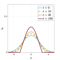
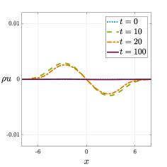
For the order of accuracy test we take as initial condition a perturbation of the steady state in (34),
| (35) |
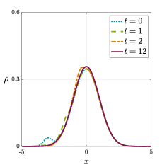
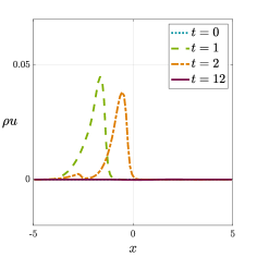
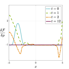
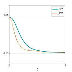
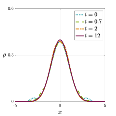
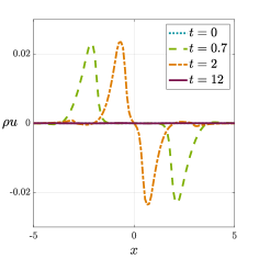
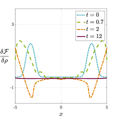
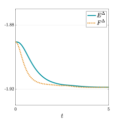
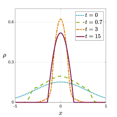
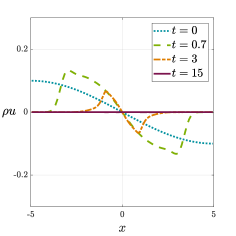
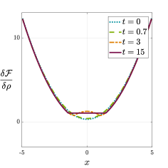
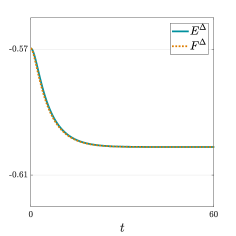
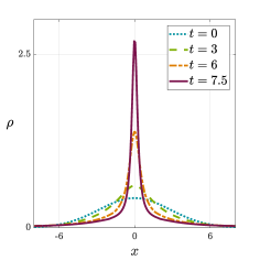
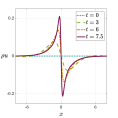
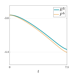
with equal to so that the total mass is also 1. The order of accuracy test from this example is shown in table 2, while the temporal evolution of the density, momentum, free-energy with respect to the density, total energy and free energy are displayed in figure 1. The third- and fifth-order of accuracy of the numerical scheme in Section 2 are evident from table 2. From figure 1 (A) we notice how the Gaussian distribution corresponding to the steady state is reached at , while in figure 1 (C) the variation of the free energy is constant throughout the domain, given that the density is not compactly supported and (10) is satisfied. Finally, it is evident from figure 1 (D) that the discrete analogs of the total energy and free energy (32) decay in time.
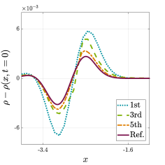
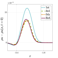
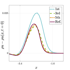
In figure 2 we visually illustrate the difference in accuracy between employing the third- and fifth-order schemes of this work versus the first-order scheme in our previous work [21], which is summarized in Subsection 2.1. We display the density and momentum fluctuation profiles at two different times ( and ), which result from substracting the initial conditions in (35) to the numerical profiles obtained with the same mesh of 100 cells for the three schemes. The choice of measuring the fluctuations with respect to the initial condition is motivated by capturing the transient behavior. We also plot a reference profile obtained with the thrid-order scheme and 12600 cells. From figure 2 we observe the benefit of employing the high-order schemes in comparison to the first-order one, since they provide a numerical solution much closer to the reference profile for the same number of cells.

Example 3.2 (Generalized Euler-Poisson system: ideal-gas pressure and attractive kernel).
For this example we select an ideal-gas free energy with pressure together with an interaction potential with a kernel of the form . In this case the steady state aimed to be preserved satisfies
| (36) |
Free energies of this type are common in Euler-Poisson systems, in which the Euler equations for a compressible gas are coupled to a self-consistent force field created by the gas particles [56]. This interaction could be gravitational, leading to the modelling of Newtonian stars [9], or electrostatic with repelling forces between the particles is is the case of plasma [54, 34]. For Euler-Poisson systems the free energy contains a function which follows a Poisson-like equation, so that
| (37) |
with being either for the gravitational case or - for the plasma one. The Poisson equation for can be solved considering the fundamental solution of the Laplacian in one dimension [62], which leads to . Then, by plugging this expression for in the variation of the free energy in (37), one recovers the interaction potential which is convoluted with the density . For a following the Poisson equation the interaction potential is , but for one can generalize it to a homogeneous kernel , where and when for convention. A popular application of these more general kernels is in the Keller-Segel system for cells and bacteria [8, 10, 19] which we explore in example 3.5.
| Number of cells | Third-order | Fifth-order | ||
|---|---|---|---|---|
| error | order | error | order | |
| 50 | 5.0109E-04 | - | 1.0913E-04 | - |
| 100 | 1.2721E-04 | 1.98 | 5.0556E-06 | 4.43 |
| 200 | 1.7573E-05 | 2.86 | 5.3713E-08 | 6.56 |
| 400 | 2.3001E-06 | 2.93 | 2.3448E-10 | 4.52 |
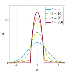
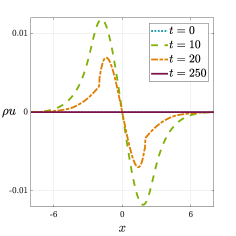
For Example 3.2 we select , leading to the interaction potential in the variation of the free energy in (36). The steady state for a general mass is equal to the steady state for example 3.1 and satisfies (34). Notice that the particular choice of and a symmetric initial condition makes this Example analytically equivalent to the case of external quadratic potential in Example 3.1 with the same initial data, just expand the convolution and use symmetry. However, by treating it numerically as a convolution we are able to check the order of accuracy for interaction potentials. For the order of accuracy test the initial condition is a symmetric perturbation of the steady state in (34),
with and equal to so that the total mass is also 1. The order of accuracy test from this example is shown in table 3, while the temporal evolution of the density, momentum, variation of the free energy with respect to the density, total energy and free energy are depicted in figure 3. The third- and fifth-order of accuracy of the numerical scheme in Section 2 are evident from table 3. Figure 3 (A) shows that the density remains symmetric at all times eventually reaching the steady state profile in (34). It is also evident from figure 3 (C) that the variation of free energy reaches a constant value in the regions where the density is non-compactly supported, while figure 3 (D) demonstrates that the total energy and free energy exhibit a temporal decay.
3.2. Numerical experiments and applications
Here we apply the finite-volume scheme we developed in Section 2 to applications of the shallow-water system, a collective behaviour system with Cucker-Smale and Motsch-Tadmor damping terms, and the Keller-Segel model. Our scheme is useful to run challenging numerical experiments for which analytical results are limited in the literature, such as in the above applications.
Example 3.3 (Shallow water: pressure proportional to square of density and attractive potential).
In this example we select a pressure satisfying together with an attractive external potential . This scenario corresponds to the well-known shallow-water equations, which model free-surface gravity waves whose wavelength is much larger than the characteristic bottom depth. The choice of leads to the presence of dry regions during the water-height evolution. These equations are applied in a wide range of engineering and scientific applications involving free-surface flows [83], such as tsunami propagation [27], dam break and flooding problems [35] and the evolution of rivers and coastal areas [33].
The main three challenges to accurately simulate the shallow-water equations are the preservation of the steady states, the preservation of the water-height positivity and the transitions between wet and dry areas. Many authors have consequently proposed various numerical schemes addressing these challenges, employing methodologies ranging from finite-difference and finite-volume schemes to discontinuous Galerkin ones. The reader can find more relevant references about high-order schemes [24], well-balanced reconstructions [3], density positivity [84] and the simulation of the wet/dry front [43] in the introduction of this work and in the comprehensive survey from Xing and Shu [83].

For this example we aim to show that our numerical scheme accurately captures the dry regions during the simulation and when reaching the steady states. This is thanks to the combination of the positive-density reconstruction in Appendix B and the choice of a kinetic numerical flux which is able to handle vacuum regions [73]. We show this by conducting simulations with two different choices for the external potential with the following initial conditions for both cases
with being the initial centre of mass. The steady states for the choice of pressure and external potentials of this example satisfy
| (38) |
where is a piecewise constant function being zero outside the support of the density.

The details of each simulation are:
-
1)
Single-well external potential and symmetric density: and . The results of this simulation are depicted in figure 4. Figure 4 (a) shows the formation of the compact support of the density during the time evolution with the steady state taking the shape of a positive parabola and satisfying (38). We also observe that the variation of the free energy in figure 4 (c) reaches a constant value only in the support of the density, in agreement with the steady-state relation in (3). We also note that in 4 (d) the discrete total energy decreases in time, while the discrete free energy has a slight increase around due to an exchange of energy with the kinetic energy.
-
2)
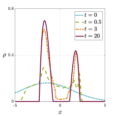
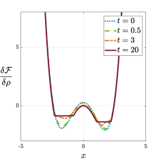
Double-well external potential and asymmetric density: and . The results of this simulation are depicted in figure 5. From the evolution of the density in figure 5 (a) it is evident that two compactly-supported bumps of density are formed when reaching the steady state. This is due to the external potential having two wells. In addition, the mass in the bumps is not the same, since the initial density is not symmetric. It is also important to remark that, when reaching the steady state, the variation of the free energy in each compacted support of the density is constant but has different values. This is depicted in figure 5 (c) and agrees with the steady state relation (3). We refer the reader to our previous work [21] for similar simulations considering varied scenarios with double-well potentials.
Example 3.4 (Collective behaviour: comparison of linear, Cucker-Smale and Motsch-Tadmor dampings).
In this example we explore the impact of adding linear and nonlinear damping terms to the general system (1). The motivation for the nonlinear damping comes from the field of collective behaviour, in which a large amount of interacting individuals or agents organize their dynamics by influencing each other and without the presence of a leader. Most of the literature in collective behaviour is based on individual based models (IBMs) which are particle descriptions considering the three basic effects of attraction, repulsion and alignment of the individuals. The combination of these three effects has proven to be very versatile and extends beyond the typical animal applications for schools of fish [58], herds of mammals [46] or flocks or birds [57]. Indeed, these models are now playing a critical role in understanding complex phenomena including consensus and spatio-temporal patterns in diverse problems ranging from the evolution of human languages [39] to the prediction of criminal behaviour [76] and space flight formation [72].
There are plenty of works in the literature addressing the mean-field derivation of kinetic and other macroscopic models from the original particle descriptions [17, 18, 55]. These derived hydrodynamic equations agree with our general system (1) and model the attraction and repulsion effects via the interaction potential . The third effect for collective behaviour is alignment which in our system (1) it is achieved by means of the nonlinear and nonlocal damping of the RHS of the momentum equation. The most popular approach for the velocity consensus is the Cucker-Smale (CS) model [37, 38] which adapts the momentum of a particle depending on the momentum and distance of the other particles. Several authors have proposed refined variations of the CS model, and among them we remark the weighted-normalized model by Motsch and Tadmor (MS) [67] (which will be referred to in the following as the MS model). It basically corrects the CS model by eliminating the normalization over the total number of agents, which leads to inaccurate behaviours in far-from-equilibrium scenarios. Instead, the MT model introduces the concept of relative distances between agents with the cost, however, of destroying the symmetry of the original CS model. For further details on flocking and alignment with the CS and related models we refer the reader to [15, 14, 66, 32].
The objective of this example is to illustrate the differences of adding to the general system (1) linear damping, the CS or the MT model. The damping term for each of them is
| (39) |
where is a nonnegative symmetric smooth function, called the communication function, satisfying for this example
It should be noted that the CS damping term in (39) would reduce to linear damping if the communication function was a constant function . In addition, the difference between the CS and MT models is the normalization over that is added to the MT model to ensure that the damping term is independent of the total mass of the system.
The simulation for this example is chosen to specifically address a particular drawback of the CS model. This occurs in the evolution of two groups of agents separated by a certain significant distance and whose masses have different degrees of magnitude. What happens with the CS model is that the damping term for the small group of agents is negligible due to the normalization over the total number of agents in the system. This means that those agents do not seek alignment from the beginning of the simulation, and as a result the convergence towards alignment is delayed. On the contrary, with the MT model the normalization over in (39) allows to take the relative distances between the agents into account, and the small group of agents reacts much faster to the effect of the rest of agents. In the simulation we also add a Morse-like interaction potential [20, 13] of the form , which quickly decays at large distances and does not add any attraction between the two groups of agents. Note that we are forced to add this attraction term to balance the pressure and thus allow for our well-balanced scheme in Section 2.
This configuration is depicted in figure 6. Specifically, figure 6 (a) and (b) shows with blue the initial conditions for the density and the momentum. On the one hand, in the density there are two groups of agents with mass of and , satisfying
while on the other hand for the momentum the two groups have opposite velocity signs, in agreement with
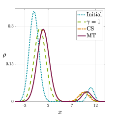

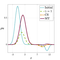

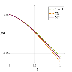
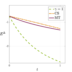
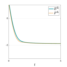
What we expect to happen in this situation is that the large group imposes its velocity sign over the small group, so eventually all the agents align with positive velocity. From the momentum simulation in figure 6 (b) we observe that after the MT model has already changed the velocity sign of the small group from negative to positive, while for the CS model the velocity is still negative. In general, linear damping is the one that dissipates more momentum, as depicted in the momentum plot of figure 6 (b) and in the total energy plot of figure 6 (d). The free energy and total energy decay are similar for both the CS and MT models. A similar numerical experiment was already conducted in [14] using particle methods.
Example 3.5 (Hydrodynamic Keller-Segel system).
The Keller-Segel model has been widely employed for chemotactic aggregation of biological populations such as cells, bacteria or insects. It models how the production of a particular chemical by these organisms leads to long-range attraction and eventually results in self-organization. Its first formulation was proposed in [59] and consisted in a drift-diffusion equation for the density (which is obtained in the overdamped limit of our system (1)) coupled with a diffusion equation for the chemical concentration.
In this example we are interested in the hydrodynamic extension of the Keller-Segel model proposed in [29] and takes into account the inertia of the biological entities and has been proposed in [29]. It follows the same structure as the generalized Euler-Poisson system in the example 3.2 with the free energy satisfying (37) and the chemical concentration usually taken as (see [19, 11]). The homogeneous kernel follows , where and when for convention. The difference with example 3.2 is that here the pressure follows with , thus allowing for compactly-supported steady states and vacuum in the density if . We refer the reader to [6] for more information about the Keller-Segel model and the diffusion equation for the chemical concentration.
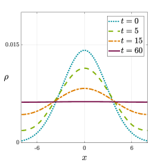
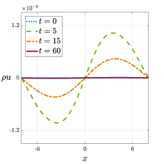
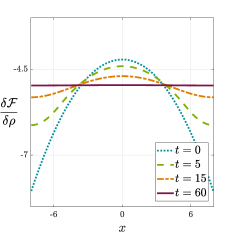
In our previous work [21] we applied our first- and second-order well-balanced scheme to investigate the competition between the attraction from the local kernel and the repulsion caused by the diffusion of the pressure . For the overdamped Keller-Segel model there are basically three possible regimes [10, 11], which result from adequately tuning the parameters in the kernel and in the pressure : diffusion dominated regime (), balanced regime () where a critical mass separates self-similar and blow-up behaviour, and aggregation-dominated regime (). Results with the momentum equation included, and thus inertia, are still quite limited in the literature, with only some specific scenarios studied [15, 22]. In our previous work [21] we investigated the role of inertia for a choice of parameters of , and , , which led to a diffusion-dominated and aggregation-dominated regimes, respectively.
For this example we aim to explore the case of which leads to the singular potential . Initially, for the two first simulations of this example we set so that . In the overdamped limit this scenario corresponds to the balanced regime since , and there is a critical mass separating the global-in-time from the finite-time blowup solution. We aim to run two simulations with identical initial conditions which differ only in a multiplicative constant for the density which allows to set a different mass of the system. The objective is to find global-in-time and finite-time blowup solutions by only changing the mass of the system. With that aim we set the initial conditions as
| (40) |
with being the mass of the system.
For the first simulation we set the mass of the system to be . The results are shown in figure 7 where the numerical solution is clearly global-in-time and diffusion-dominated. Eventually the steady state is reached,
From figure 7 (a) we observe that the solution is completely diffused and the final profile for the density is uniform. From figure 7 (c) we notice that the variation of the free energy with respect to the density is constant once the steady state is reached, and from figure 7 (d) we remark how the total and free energy decay during the temporal evolution.

For the second simulation we select a mass of while keeping the same initial conditions as in (40). As displayed in figure 8, the solution now presents a finite-time blowup around , leading to an aggregation-dominated behaviour. Figure 8 (a) reveals that the density is concentrated towards the middle of the domain while figure 8 (b) shows that the momentum presents an infinite slope when reaching the blowup. From figure 8 (d) we notice that the total and free energy temporally decay until the blowup occurs.
Finally, we also aim to compare diffusion-dominated solutions where leading to steady states that are compactly supported. For this purpose we set the initial conditions to be (40) with a mass of . For comparison we look at two scenarios with and so that the exponent is different. In figure 9 we depict the final steady states that arise from the two choices of . From figures 9 (a) and (c) we observe that the final compactly-supported density profiles have slightly different shapes due to the balances between the attraction from the local kernel and the repulsion caused by the diffusion of the pressure .
Acknowledgements
José A. Carrillo was partially supported by EPSRC grant number EP/P031587/1. Manuel J. Castro acknowledges financial support from the Spanish Government and FEDER through the coordinated Research project RTI2018-096064-B-C21 and from Junta de Andalucía and FEDER through the project UMA18-FEDERJA-161. Serafim Kalliadasis acknowledges financial support from the Engineering and Physical Sciences Research Council (EPSRC) of the UK through Grant No. EP/L020564. And Sergio P. Perez acknowledges financial support from the Imperial College President’s PhD Scholarship and thanks Universidad de Málaga for hospitality during a visit in October 2019.
Appendix A Details about the fifth-order Gaussian quadrature
In this section we detail the procedure to approximate an integral via the fifth-order Gaussian quadrature. Briefly, Gaussian quadratures of points yield exact values of integrals for polynomials of degree up to . In our case we implement Gaussian quadratures of points, so that the spatial error is of the order . In this way we do not limit the order of the high-order finite volume schemes, since the order of this quadrature is always higher or equal than ones in the reconstructions of the scheme.
The approximation of a function within an interval via a three-point Gaussian quadrature [1] satisfies
In our case, this integration is performed within each of the finite volume cells in centred at and with size . The cell averages in the finite volume schemes are also divided over . As a result, the transformation of weights and spatial coordinates for the Gaussian quadrature from to results in
From this last expression we get that the coefficients for satisfy
with the spatial nodes within the cell for the evaluations of the integrand located at
Appendix B Details about the positive-density CWENO reconstruction
In this section we proceed to summarize the third- and fifth-order CWENO reconstructions of a generic function whose cell averages , defined as in (8), are taken as input. Each cell has size , is centred at and is contained in the region . These reconstructions are applied in (19) to compute the high-order reconstructions , and . For further details about the CWENO algorithm, we refer the reader to [36, 64, 63, 12].
In subsection B.1 we detail the third-order reconstruction, in subsection B.2 we proceed with the fifth-order reconstruction, and finally in subsection B.3 we end up by summarizing the positive-density limiters from [84], which are essential to prove the positivity of the overall finite volume scheme.
B.1. Third-order CWENO reconstruction
The third-order CWENO reconstruction from [63] satisfies
| (41) |
with , and resulting from
| (42) |
and , and , for , being computed as
The weights appearing in (42), for , satisfy
| (43) |
The constants , , , and for in (43) are
| (44) |
Finally, the smoothness indicators for in (43), where , result from
| (45) |
The proposed choice of the constants in (44) and the smoothness indicators in (45) is based on the original work for third-order CWENO reconstruction in [63]. The reader can find about other more refined choices in [64] and later works [74, 2, 61, 36].
B.2. Fifth-order CWENO reconstruction
The fifth-order CWENO reconstruction from [12] satisfies
| (46) |
with , , , and resulting from
| (47) |
The coefficients for which appear in the optimal polynomial in (47) are taken as
The rest of the coefficients , and for which appear in the polynomials , and , respectively, follow from
The weights for in the fifth-order CWENO reconstruction (46) satisfy
| (48) |
The constants , , , , and for in (48) are
Finally, the smoothness indicators which appear in the computation of in (48), with , result from
B.3. Positive-density CWENO reconstruction
The third- and fifth-order CWENO reconstructions in (41) or (46), respectively, can be modified to yield positive values for evaluations at specific spatial points of the finite volume cell. In our case we are interested in obtaining positive values of the density at the points required by the numerical scheme in (27). Namely, those points are: the boundaries of the cell, computed in (28) and employed for in (29), (30) and (31), and the quadrature points to compute the integrals in the nonlinear damping term in (27), the distribution of the high-order corrections in the source term in (27) and described in appendix C, and the update of in (26). We refer the reader to the appendices A and C for the details of the location of the quadrature points.
Zhang and Shu [84] proposed a methodology to construct maximum-principle-satisfying high-order schemes. Here we apply their work in [84] to modify the CWENO reconstructions in the subsections B.1 and B.2, so that they preserve the positivity of the density. The procedure is the following:
- 1)
-
2)
Evaluate the reconstructed polynomials at the spatial points required by the numerical scheme in (27): the boundaries of the cells and quadrature points. We denote as the total number those spatial points.
-
3)
For each cell compute the minimum of the evaluations of the reconstructed polynomial at the required spatial points , for , so that .
- 4)
-
5)
Evaluate all the spatial points within each cell with the modified reconstructed polynomial .
-
6)
Apply the following CFL condition for the time step , depending on the numerical flux employed and where is the quadrature weight of the spatial point , for :
(49) The quadrature weights employed in this work are specified in the appendices A and C. For the details about the numerical fluxes we refer the reader to our previous work [21].
Appendix C Details about the integration for the high-order corrections
In this section we follow [70, 71] to propose a fourth- and sixth-order quadrature for the high-order corrections in the source term, which appear in the last term of (27) and satisfy
| (50) |
The first step is to define a general trapezoidal numerical quadrature for the integral in (50), which employs points of the cell , with . Such integral yields
| (51) |
The integral is a second-order approximation of in (50), and its asymptotic form satisfies [70]
| (52) |
The strategy to obtain the fourth- and sixth-order schemes relies in computing the integral in (50) as a linear combination of for different , such that the desired errors in (52) are cancelled. The required formulas of integration are:
-
a)
Fourth-order quadrature employing and , so that
-
b)
Sixth-order quadrature employing , and , so that
As a remark, the order of these quadratures is maintained as long as the order of the reconstructions for the density in (19) and the potential in (20) is greater than or at least equal to the order of the quadrature formulas. Otherwise the order of the quadrature is diminished and matches the order of the reconstruction.
References
- [1] M. Abramowitz, I. A. Stegun, and R. H. Romer, Handbook of mathematical functions with formulas, graphs, and mathematical tables, 1988.
- [2] F. Aràndiga, A. Baeza, A. Belda, and P. Mulet, Analysis of WENO schemes for full and global accuracy, SIAM Journal on Numerical Analysis, 49 (2011), pp. 893–915.
- [3] E. Audusse, F. Bouchut, M.-O. Bristeau, R. Klein, and B. t. Perthame, A fast and stable well-balanced scheme with hydrostatic reconstruction for shallow water flows, SIAM Journal on Scientific Computing, 25 (2004), pp. 2050–2065.
- [4] E. Audusse, C. Chalons, and P. Ung, A very simple well-balanced positive and entropy-satisfying scheme for the shallow-water equations, Commun. Math. Sci, 13 (2015), pp. 1317–1332.
- [5] R. Bailo, J. A. Carrillo, and J. Hu, Fully discrete positivity-preserving and energy-decaying schemes for aggregation-diffusion equations with a gradient flow structure, Preprint arxiv, 2018 (1811).
- [6] N. Bellomo, A. Bellouquid, Y. Tao, and M. Winkler, Toward a mathematical theory of Keller–Segel models of pattern formation in biological tissues, Mathematical Models and Methods in Applied Sciences, 25 (2015), pp. 1663–1763.
- [7] A. Bermúdez and M. E. Vázquez, Upwind methods for hyperbolic conservation laws with source terms, Computers & Fluids, 23 (1994), pp. 1049–1071.
- [8] S. Bian and J.-G. Liu, Dynamic and steady states for multi-dimensional Keller-Segel model with diffusion exponent , Communications in Mathematical Physics, 323 (2013), pp. 1017–1070.
- [9] J. Binney and S. Tremaine, Galactic dynamics, Princeton university press, 2011.
- [10] V. Calvez, J. A. Carrillo, and F. Hoffmann, Equilibria of homogeneous functionals in the fair-competition regime, Nonlinear Analysis, 159 (2017), pp. 85–128.
- [11] V. Calvez, J. A. Carrillo, and F. Hoffmann, The geometry of diffusing and self-attracting particles in a one-dimensional fair-competition regime, in Nonlocal and nonlinear diffusions and interactions: new methods and directions, Springer, 2017, pp. 1–71.
- [12] G. Capdeville, A central WENO scheme for solving hyperbolic conservation laws on non-uniform meshes, Journal of Computational Physics, 227 (2008), pp. 2977–3014.
- [13] J. A. Carrillo, A. Chertock, and Y. Huang, A finite-volume method for nonlinear nonlocal equations with a gradient flow structure, Communications in Computational Physics, 17 (2015), pp. 233–258.
- [14] J. A. Carrillo, Y.-P. Choi, and S. P. Perez, A review on attractive–repulsive hydrodynamics for consensus in collective behavior, in Act. Part. Vol. 1, Springer, 2017, pp. 259–298.
- [15] J. A. Carrillo, Y.-P. Choi, E. Tadmor, and C. Tan, Critical thresholds in 1d Euler equations with non-local forces, Mathematical Models and Methods in Applied Sciences, 26 (2016), pp. 185–206.
- [16] J. A. Carrillo, E. Feireisl, P. Gwiazda, and A. Świerczewska-Gwiazda, Weak solutions for Euler systems with non-local interactions, Journal of the London Mathematical Society, 95 (2017), pp. 705–724.
- [17] J. A. Carrillo, M. Fornasier, J. Rosado, and G. Toscani, Asymptotic flocking dynamics for the kinetic cucker–smale model, SIAM Journal on Mathematical Analysis, 42 (2010), pp. 218–236.
- [18] J. A. Carrillo, M. Fornasier, G. Toscani, and F. Vecil, Particle, kinetic, and hydrodynamic models of swarming, in Mathematical modeling of collective behavior in socio-economic and life sciences, Springer, 2010, pp. 297–336.
- [19] J. A. Carrillo, F. Hoffmann, E. Mainini, and B. Volzone, Ground states in the diffusion-dominated regime, Calculus of variations and partial differential equations, 57 (2018), p. 127.
- [20] J. A. Carrillo, Y. Huang, and S. Martin, Explicit flock solutions for quasi-morse potentials, European Journal of Applied Mathematics, 25 (2014), pp. 553–578.
- [21] J. A. Carrillo, S. Kalliadasis, S. P. Perez, and C.-W. Shu, Well-balanced finite volume schemes for hydrodynamic equations with general free energy, 2020. to appear.
- [22] J. A. Carrillo, A. Wróblewska-Kamińska, and E. Zatorska, On long-time asymptotics for viscous hydrodynamic models of collective behavior with damping and nonlocal interactions, Mathematical Models and Methods in Applied Sciences, 29 (2018), pp. 31–63.
- [23] M. J. Castro, T. M. de Luna, and C. Parés, Well-balanced schemes and path-conservative numerical methods, in Handbook of Numerical Analysis, vol. 18, Elsevier, 2017, pp. 131–175.
- [24] M. J. Castro, J. A. López-García, and C. Parés, High order exactly well-balanced numerical methods for shallow water systems, Journal of Computational Physics, 246 (2013), pp. 242 – 264.
- [25] M. J. Castro, A. Pardo Milanés, and C. Parés, Well-balanced numerical schemes based on a generalized hydrostatic reconstruction technique, Mathematical Models and Methods in Applied Sciences, 17 (2007), pp. 2055–2113.
- [26] M. J. Castro and C. Parés, Well-balanced high-order finite volume methods for systems of balance laws, Journal of Scientific Computing, 82 (2020), p. 48.
- [27] M. J. Castro and M. Semplice, Third-and fourth-order well-balanced schemes for the shallow water equations based on the CWENO reconstruction, International Journal for Numerical Methods in Fluids, 89 (2019), pp. 304–325.
- [28] C. Chalons, P. Goatin, and L. M. Villada, High-order numerical schemes for one-dimensional nonlocal conservation laws, SIAM Journal on Scientific Computing, 40 (2018), pp. A288–A305.
- [29] P.-H. Chavanis and C. Sire, Kinetic and hydrodynamic models of chemotactic aggregation, Physica A: Statistical Mechanics and its Applications, 384 (2007), pp. 199–222.
- [30] Y. Cheng, A. Chertock, M. Herty, A. Kurganov, and T. Wu, A new approach for designing moving-water equilibria preserving schemes for the shallow water equations, Journal of Scientific Computing, 80 (2019), pp. 538–554.
- [31] A. Chertock, S. Cui, A. Kurganov, Ş. N. Özcan, and E. Tadmor, Well-balanced schemes for the Euler equations with gravitation: Conservative formulation using global fluxes, Journal of Computational Physics, 358 (2018), pp. 36–52.
- [32] Y.-P. Choi, S.-Y. Ha, and Z. Li, Emergent dynamics of the cucker–smale flocking model and its variants, in Active Particles, Volume 1, Springer, 2017, pp. 299–331.
- [33] V. Churuksaeva and A. Starchenko, Mathematical modeling of a river stream based on a shallow water approach, Procedia Computer Science, 66 (2015), pp. 200–209.
- [34] S. Cordier and E. Grenier, Quasineutral limit of an Euler-Poisson system arising from plasma physics, Communications in Partial Differential Equations, 25 (2000), pp. 1099–1113.
- [35] L. Cozzolino, V. Pepe, L. Cimorelli, A. D’Aniello, R. Della Morte, and D. Pianese, The solution of the dam-break problem in the porous shallow water equations, Advances in Water Resources, 114 (2018), pp. 83–101.
- [36] I. Cravero and M. Semplice, On the accuracy of WENO and CWENO reconstructions of third order on nonuniform meshes, Journal of Scientific Computing, 67 (2016), pp. 1219–1246.
- [37] F. Cucker and S. Smale, Emergent behavior in flocks, IEEE Transactions on Automatic Control, 52 (2007), pp. 852–862.
- [38] , On the mathematics of emergence, Japanese J. Math., 2 (2007), pp. 197–227.
- [39] F. Cucker, S. Smale, and D.-X. Zhou, Modeling language evolution, Foundations of Computational Mathematics, 4 (2004), pp. 315–343.
- [40] F. Filbet, A finite volume scheme for the Patlak–Keller–Segel chemotaxis model, Numerische Mathematik, 104 (2006), pp. 457–488.
- [41] F. Filbet and C.-W. Shu, Approximation of hyperbolic models for chemosensitive movement, SIAM Journal on Scientific Computing, 27 (2005), pp. 850–872.
- [42] U. S. Fjordholm, S. Mishra, and E. Tadmor, Arbitrarily high-order accurate entropy stable essentially nonoscillatory schemes for systems of conservation laws, SIAM Journal on Numerical Analysis, 50 (2012), pp. 544–573.
- [43] J. M. Gallardo, C. Parés, and M. J. Castro, On a well-balanced high-order finite volume scheme for shallow water equations with topography and dry areas, Journal of Computational Physics, 227 (2007), pp. 574–601.
- [44] A. Gamba, D. Ambrosi, A. Coniglio, A. De Candia, S. Di Talia, E. Giraudo, G. Serini, L. Preziosi, and F. Bussolino, Percolation, morphogenesis, and Burgers dynamics in blood vessels formation, Physical Review Letters, 90 (2003), p. 118101.
- [45] L. Gascón and J. Corberán, Construction of second-order tvd schemes for nonhomogeneous hyperbolic conservation laws, Journal of computational physics, 172 (2001), pp. 261–297.
- [46] I. Giardina, Collective behavior in animal groups: theoretical models and empirical studies, HFSP journal, 2 (2008), pp. 205–219.
- [47] J. Giesselmann, C. Lattanzio, and A. E. Tzavaras, Relative energy for the Korteweg theory and related Hamiltonian flows in gas dynamics, Archive for Rational Mechanics and Analysis, 223 (2017), pp. 1427–1484.
- [48] B. D. Goddard, A. Nold, N. Savva, P. G. A, and S. Kalliadasis, General dynamical density functional theory for classical fluids, Physical Review Letters, 109 (2012), p. 120603.
- [49] B. D. Goddard, A. Nold, N. Savva, P. Yatsyshin, and S. Kalliadasis, Unification of dynamic density functional theory for colloidal fluids to include inertia and hydrodynamic interactions: derivation and numerical experiments, Journal of Physics: Condensed Matter, 25 (2012), p. 35101.
- [50] L. Gosse, A well-balanced flux-vector splitting scheme designed for hyperbolic systems of conservation laws with source terms, Computers & Mathematics with Applications, 39 (2000), pp. 135–159.
- [51] L. Gosse, Asymptotic-preserving and well-balanced schemes for the 1d cattaneo model of chemotaxis movement in both hyperbolic and diffusive regimes, Journal of Mathematical Analysis and Applications, 388 (2012), pp. 964–983.
- [52] S. Gottlieb and C.-W. Shu, Total variation diminishing Runge-Kutta schemes, Math. Comput. Am. Math. Soc., 67 (1998), pp. 73–85.
- [53] J. M. Greenberg and A.-Y. LeRoux, A well-balanced scheme for the numerical processing of source terms in hyperbolic equations, SIAM Journal on Numerical Analysis, 33 (1996), pp. 1–16.
- [54] Y. Guo and B. Pausader, Global smooth ion dynamics in the Euler-Poisson system, Communications in Mathematical Physics, 303 (2011), pp. 89–125.
- [55] S.-Y. Ha and E. Tadmor, From particle to kinetic and hydrodynamic descriptions of flocking, Kinetic & Related Models, 1 (2008), p. 415.
- [56] M. Hadžić and J. J. Jang, A class of global solutions to the Euler–Poisson system, Communications in Mathematical Physics, 370 (2019), pp. 475–505.
- [57] H. Hildenbrandt, C. Carere, and C. K. Hemelrijk, Self-organized aerial displays of thousands of starlings: a model, Behavioral Ecology, 21 (2010), pp. 1349–1359.
- [58] Y. Katz, K. Tunstrøm, C. C. Ioannou, C. Huepe, and I. D. Couzin, Inferring the structure and dynamics of interactions in schooling fish, Proceedings of the National Academy of Sciences, 108 (2011), pp. 18720–18725.
- [59] E. F. Keller and L. A. Segel, Initiation of slime mold aggregation viewed as an instability, Journal of theoretical biology, 26 (1970), pp. 399–415.
- [60] C. Klingenberg, G. Puppo, and M. Semplice, Arbitrary order finite volume well-balanced schemes for the Euler equations with gravity, SIAM Journal on Scientific Computing, 41 (2019), pp. A695–A721.
- [61] O. Kolb, On the full and global accuracy of a compact third order WENO scheme, SIAM Journal on Numerical Analysis, 52 (2014), pp. 2335–2355.
- [62] C. Lattanzio and A. E. Tzavaras, From gas dynamics with large friction to gradient flows describing diffusion theories, Communications in Partial Differential Equations, 42 (2017), pp. 261–290.
- [63] D. Levy, G. Puppo, and G. Russo, Central WENO schemes for hyperbolic systems of conservation laws, ESAIM: Mathematical Modelling and Numerical Analysis, 33 (1999), pp. 547–571.
- [64] , Compact central WENO schemes for multidimensional conservation laws, SIAM Journal on Scientific Computing, 22 (2000), pp. 656–672.
- [65] F. Marche, P. Bonneton, P. Fabrie, and N. Seguin, Evaluation of well-balanced bore-capturing schemes for 2d wetting and drying processes, International Journal for Numerical Methods in Fluids, 53 (2007), pp. 867–894.
- [66] P. Minakowski, P. B. Mucha, J. Peszek, and E. Zatorska, Singular cucker–smale dynamics, in Active Particles, Volume 2, Springer, 2019, pp. 201–243.
- [67] S. Motsch and E. Tadmor, A new model for self-organized dynamics and its flocking behavior, Journal of Statistical Physics, 144 (2011), p. 923.
- [68] R. Natalini and M. Ribot, Asymptotic high order mass-preserving schemes for a hyperbolic model of chemotaxis, SIAM Journal on Numerical Analysis, 50 (2012), pp. 883–905.
- [69] R. Natalini, M. Ribot, and M. Twarogowska, A well-balanced numerical scheme for a one dimensional quasilinear hyperbolic model of chemotaxis, arXiv preprint arXiv:1211.4010, (2012).
- [70] S. Noelle, N. Pankratz, G. Puppo, and J. R. Natvig, Well-balanced finite volume schemes of arbitrary order of accuracy for shallow water flows, Journal of Computational Physics, 213 (2006), pp. 474–499.
- [71] S. Noelle, Y. Xing, and C.-W. Shu, High-order well-balanced finite volume WENO schemes for shallow water equation with moving water, Journal of Computational Physics, 226 (2007), pp. 29–58.
- [72] L. Perea, G. Gómez, and P. Elosegui, Extension of the cucker-smale control law to space flight formations, Journal of guidance, control, and dynamics, 32 (2009), pp. 527–537.
- [73] B. Perthame and C. Simeoni, A kinetic scheme for the Saint-Venant system with a source term, Calcolo, 38 (2001), pp. 201–231.
- [74] M. Semplice, A. Coco, and G. Russo, Adaptive mesh refinement for hyperbolic systems based on third-order compact WENO reconstruction, Journal of Scientific Computing, 66 (2016), pp. 692–724.
- [75] G. Serini, D. Ambrosi, E. Giraudo, A. Gamba, L. Preziosi, and F. Bussolino, Modeling the early stages of vascular network assembly, The EMBO journal, 22 (2003), pp. 1771–1779.
- [76] M. B. Short, M. R. D’orsogna, V. B. Pasour, G. E. Tita, P. J. Brantingham, A. L. Bertozzi, and L. B. Chayes, A statistical model of criminal behavior, Mathematical Models and Methods in Applied Sciences, 18 (2008), pp. 1249–1267.
- [77] C.-W. Shu, Essentially non-oscillatory and weighted essentially non-oscillatory schemes for hyperbolic conservation laws, tech. rep., 1997.
- [78] C.-W. Shu and S. Osher, Efficient implementation of essentially non-oscillatory shock-capturing schemes, Journal of Computational Physics, 77 (1988), pp. 439–471.
- [79] , Efficient implementation of essentially non-oscillatory shock-capturing schemes, II, Journal of Computational Physics, 83 (1989), pp. 32–78.
- [80] E. Tadmor, Entropy stable schemes, in Handbook of Numerical Analysis, vol. 17, Elsevier, 2016, pp. 467–493.
- [81] A. Thomann, M. Zenk, and C. Klingenberg, A second-order positivity-preserving well-balanced finite volume scheme for Euler equations with gravity for arbitrary hydrostatic equilibria, International Journal for Numerical Methods in Fluids, 89 (2019), pp. 465–482.
- [82] Y. Xing and C.-W. Shu, High order well-balanced finite volume WENO schemes and discontinuous Galerkin methods for a class of hyperbolic systems with source terms, Journal of Computational Physics, 214 (2006), pp. 567–598.
- [83] , A survey of high order methods for the shallow water equations, Journal of Mathematical Study, 47 (2014).
- [84] X. Zhang and C.-W. Shu, On maximum-principle-satisfying high order schemes for scalar conservation laws, Journal of Computational Physics, 229 (2010), pp. 3091–3120.