Shape Estimation for Elongated Deformable Object using B-spline Chained Multiple Random Matrices Model

Abstract

In this paper, a B-spline chained multiple random matrices representation is proposed to model geometric characteristics of an elongated deformable object. The hyper degrees of freedom structure of the elongated deformable object make its shape estimation challenging. Based on the likelihood function of the proposed model, an expectation-maximization (EM) method is derived to estimate the shape of the elongated deformable object. A split and merge method based on the Euclidean minimum spanning tree (EMST) is proposed to provide initialization for the EM algorithm. The proposed algorithm is evaluated for the shape estimation of the elongated deformable objects in scenarios, such as the static rope with various configurations (including configurations with intersection), the continuous manipulation of a rope and a plastic tube, and the assembly of two plastic tubes. The execution time is computed and the accuracy of the shape estimation results is evaluated based on the comparisons between the estimated width values and its ground-truth, and the intersection over union (IoU) metric.

1 Introduction

Elongated deformable objects are deformable objects which are characterized by a length that is much longer than their width shah2018planning ; zea2016tracking . Objects of this type are commonly encountered in daily life, such as ropes, tubes, and trains. Automatic manipulation tasks such as grasping, completing surgical sutures or assembling cable harnesses are challenging due to the hyper degrees of freedom structure of the elongated deformable objects sanchez2018robotic ; shah2018planning ; jackson2017real . To improve the manipulation performance, it is necessary to provide an accurate perception model of the elongated deformable object as feedback to the robotic manipulators. The shape estimation of the elongated deformable object using data collected from the perception sensors, such as RGB-D cameras, is a challenging problem. In this paper, a shape estimation methodology for elongated deformable objects using a chained multiple random matrices representation is developed.

   

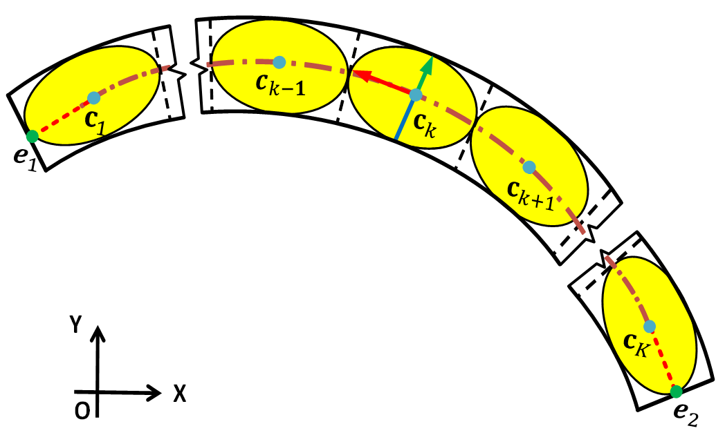
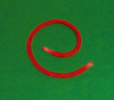
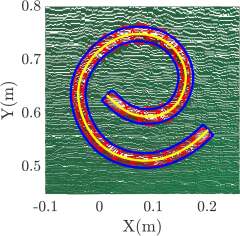
Figure 1: (a) Representation of an elongated deformable object as a B-spline curve chained multiple random matrices model; (b) The RGB image of the rope; (c) The point cloud and the shape estimation result of the rope, where the red ellipses are chained by the yellow B-spline curve and the blue curves are the offset curves from the B-spline.

Some works use the physics-based simulation models such as linked capsules tang2018track ; schulman2013tracking , mass-spring models or finite element method model petit2015real to represent the elongated deformable object by considering the physical constraints of the object shah2018planning ; tang2018track ; petit2015real ; schulman2013tracking ; javdani2011modeling . A variety of registration algorithms are used to find the correspondences between the measurements and the predefined nodes on the simulated physics model. For example, the Gaussian mixture model (GMM) incorporating coherent point drift regularization is applied to register the rope nodes of a dynamic simulation model to the noisy point cloud, using a stereo camera in tang2018track . The iterative closest point (ICP) method is used to estimate the rigid transformation from a point cloud to a 3D volumetric mesh, generated by the finite element method in petit2015real . A modified expectation-maximization (EM) algorithm is designed to directly register a point cloud from an RGB-D camera to a predefined mechanical model by a physical simulator in schulman2013tracking . However, the physical simulation models only work for linked rigid objects or elastic objects. The accuracy of the algorithms depends on the physics-based prior and the physical simulation. A physically accurate model is used in javdani2011modeling to model the elongated deformable object, and the physics-based priors are estimated by minimizing a generic energy function based on the images from a calibrated 3-camera rig.

Elongated deformable objects are also modeled by graphs or splines in DeGregorio ; lui2013tangled . A linear graph (line segments and not the shape) is used to represent a rope, and particle filters based on a predefined score function are used to infer the rope configuration in lui2013tangled . A region adjacency graph based on the super-pixels from the image of wires is developed to model the elongated deformable object in DeGregorio . A method based on topological model and knot theory is developed to recognize the rope conditions in matsuno2006manipulation . Based on the point cloud from an RGB-D camera, Bézier curve chained rectangles are used to approximate an elongated deformable object, the corresponding likelihood function is proposed, and the progressive Gaussian filter is used for the state estimation in zea2016tracking . However, the paper doesn’t consider the situation where the elongated deformable object intersects with itself. A nonuniform rational B-spline (NURBS) curve is used to model a thin, deformable surgical suture thread by minimizing the image matching energy between the projected stereo NURBS image and the segmented thread image jackson2017real .

In this paper, an elongated deformable object is modeled as chained ellipses as shown in Fig. 1 (a), where the centers of the ellipses are located on a B-spline curve (brown dash-dotted line). Each ellipse (in yellow) is represented by a random matrix model (RMM), of which the center represents the location and the covariance matrix represents the shape of the ellipse. The RMM approximation of an elliptical object is widely used for extended object tracking. Extended object tracking methods track the position of the centroid and estimate the shape of the object, given sparse point measurements on the object at each time frame (cf. yao2017image ; yao2018image ; feldmann2011tracking ). The proposed method is based on the point cloud of the elongated deformable object obtained by an RGB-D camera. The point cloud generated from the elongated deformable object is sparse but provides the position information which can be used as the measurements.

The B-spline chained RMMs can also be used when both the shape and the length of the object are changing, e.g. during the manipulations, or when assembling two elongated deformable objects. In addition, the physical simulation model of the elongated deformable object is not required to be built beforehand. Technical contributions of the paper are briefly summarized as follows:

• A set of chained multiple RMMs is proposed to approximate the elongated deformable object, of which the centers are enforced to be located on a B-spline curve. The corresponding likelihood function is derived. The proposed model both localizes the elongated deformable object and estimates its shape.

• A modified EM algorithm is proposed for the shape estimation of the elongated deformable object, based on the proposed log-likelihood function. The control points of the B-spline curve, the number of measurement points associated with each RMM and the covariance matrices of the RMMs are the parameters to be estimated by the EM algorithm.

• Because the log-likelihood function is nonconvex, it is necessary to have a good initialization for the EM algorithm. Knot sequence of the B-spline curve also needs to be generated from the unordered measurement points. A split and merge algorithm is proposed for the initialization which uses the Euclidean minimum spanning tree (EMST) and the breadth first search (BFS) method.

The rest of the paper is organized as follows. In Section 2, the B-spline curve chained RMMs, its likelihood function and a corresponding EM method are presented to estimate the position and shape of the elongated deformable object. In Section 3, a split and merge method based on the EMST and BFS is proposed to initialize the chained RMMs. The shape estimation results of the rope in different configurations, including non-intersection and intersection, based on measurements from the RGB-D camera, are shown in Section 4. The estimation results of the rope as well as the plastic tube in scenarios such as continuous manipulations and the assembly of two plastic tubes are also shown in this section. Conclusions and future work are given in Section 5.

2 B-spline Chained Random Matrices Model

2.1 B-spline Curve Representation

A point $\mathbf{p}(t)\in\mathbb{R}^{2\times 1}$ on the B-spline curve of degree $d$ can be interpolated with parameter $t$ from a polynomial, which is defined as a linear combination of $n+1$ control points (de Boor points) $\mathbf{b}_{i}\in\mathbb{R}^{2\times 1}$ and basis functions $N_{i,d}$ given by de1978practical

$$\begin{array}[]{c}\begin{aligned} \mathbf{p}(t)&=\sum_{i=0}^{n}\text{$\mathbf{b}$}_{i}N_{i,d}(t)\end{aligned}\\ 0\leq t\leq n-d+1\end{array}$$ (1)

The basis function $N_{i,d}(t)$ is defined based on a non-decreasing knot sequence $\left\{t_{i}\colon i=0\cdots n+d+1\right\}$ as de1978practical

$$N_{i,d}(t)=\frac{t-t_{i}}{t_{i+d}-t_{i}}N_{i,d-1}(t)+\frac{t_{i+d+1}-t}{t_{i+d+1}-t_{i+1}}N_{i+1,d-1}(t)$$ (2)

which is a recursion function and

$$N_{i,0}(t)=\begin{cases}1&t\in\left[t_{i},t_{i+1}\right)\\ 0&otherwise\end{cases}$$ (3)

and the knot values $t_{i}$ of the knot sequence are generated by

$$t_{i}=\begin{cases}0&0\leq i<d+1\\ i-d&d+1\leq i\leq n\\ n-d+1&n<i\leq n+d+1\end{cases}$$ (4)

2.2 Chained Multiple Random Matrices Model

  

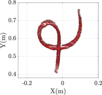
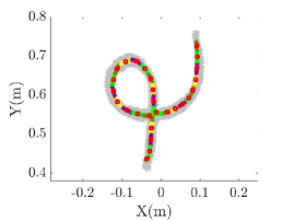
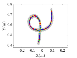
Figure 2: Illustration of the initialization procedure: (a) Point cloud from the rope after background subtraction; (b) EMST of the points, the longest path (orange line segments) and the common vertex (in cyan); (c) Small segments represented by different colors and the corresponding centers (red points); (d) Graph of centers (blue line segments) and the common vertex and its 4 closest centers (in cyan).

The B-spline chained multiple random matrices model is used to model the elongated deformable object in this section as shown in Fig. 1. The multiple random matrices model is the sum of equally weighted $K$ RMMs, which is defined as

$$p(\mathbf{Z}\mid\theta)=\sum_{k=1}^{K}w_{k}\phi(\mathbf{Z}_{k}|L_{k},\mu_{k},\Sigma_{k})$$ (5)

where $\theta=\left\{\left(L_{k},\mu_{k},\Sigma_{k}\right)\right\}_{k=1}^{K}$, $L_{k}$ is the number of measurements assigned to the $k\textrm{th}$ RMM, $\mu_{k}$ and $\Sigma_{k}$ are the mean and covariance of the $k\textrm{th}$ cluster, $\phi(\mathbf{Z}_{k}|L_{k},\mu_{k},\Sigma_{k})$ is the probability distribution of the measurement points $\mathbf{Z}_{k}=\{\mathbf{z}_{k,l}\}_{l=1}^{L_{k}}$ from the $k\textrm{th}$ cluster, $\mathbf{Z}=\{\mathbf{z}_{r}\}_{r=1}^{N_{r}}$ is the set of total number of measurement points, and the weights of the clusters are assumed to be equal as $w_{k}=\frac{1}{K}$.

The $k\textrm{th}$ cluster is approximated as an ellipse, and the measurement points inside the ellipse are assumed to be distributed as a Gaussian distribution with mean $\mu_{k}$ and covariance $\Sigma_{k}$. The probability of the measurement points $\mathbf{Z}_{k}=\{\mathbf{z}_{k,l}\}_{l=1}^{L_{k}}$ from the $k\textrm{th}$ ellipse represented by RMM is feldmann2011tracking

$$\phi(\mathbf{Z}_{k}|L_{k},\mu_{k},\Sigma_{k}) =\prod_{l=1}^{L_{k}}\mathcal{N}(\mathbf{z}_{k,l};\mu_{k},\Sigma_{k})$$ (6)

$$\propto\mathcal{N}(\mathbf{\overline{z}}_{k};\mu_{k},\frac{\Sigma_{k}}{L_{k}})\times W(\mathbf{\overline{C}}_{k};L_{k}-1,\Sigma_{k})$$

where the center $\mathbf{\overline{z}}_{k}$ is

$$\mathbf{\overline{z}}_{k}=\frac{1}{L_{k}}\sum_{l=1}^{L_{k}}\mathbf{z}_{k,l}$$ (7)

and the scattering matrix $\mathbf{\overline{C}}_{k}$ is

$$\mathbf{\overline{C}}_{k}=\sum_{l=1}^{L_{k}}(\mathbf{z}_{k,l}-\mathbf{\overline{z}}_{k,l})(\mathbf{z}_{k,l}-\mathbf{\overline{z}}_{k,l})^{\mathrm{T}}$$ (8)

and $W(\mathbf{\overline{C}}_{k};L_{k}-1,\Sigma_{k})$ is a Wishart density in $\mathbf{\overline{C}}_{k}$ with $L_{k}-1$ degrees of freedom. The statistical sensor errors are assumed to be neglected, and the physical extension of the target dominates the spread of measurements in (6) feldmann2011tracking . If the sensor errors are within the same order of the magnitude of the target extension, they cannot be neglected anymore. In this case, the covariance is $\Sigma_{k}=\Sigma_{p}+\boldsymbol{\mathbf{R}}$, where $\Sigma_{p}$ is a symmetric positive definite random matrix representing the physical extension, and $\mathbf{R}$ is the covariance matrix of sensor errors feldmann2011tracking .

The brown dash-dotted curve in Fig. 1 (a) is the B-spline curve, which crosses through the centers of the clusters. Multiple RMMs with centers located on the B-spline curve constitute the elongated deformable object. The probability of the measurement points $\mathbf{Z}_{k}=\{\mathbf{z}_{k,l}\}_{l=1}^{L_{k}}$ from the $k\textrm{th}$ elliptical cluster is defined as

$$\phi(\mathbf{Z}_{k}|L_{k},\text{$\mathbf{c}$}_{k},\Sigma_{k})= \intop_{\mu_{k}}\phi(\mathbf{Z}_{k}|L_{k},\mu_{k},\Sigma_{k})\cdot p(\mu_{k}|\mathbf{c}_{k})d\mu_{k}$$ (9)

where $\phi(\mathbf{Z}_{k}|L_{k},\text{$\mathbf{c}$}_{k},\Sigma_{k})$ is the probability distribution of the measurement points from the $k\textrm{th}$ cluster and $p(\mu_{k}|\mathbf{c}_{k})=\delta(\mu_{k}-\mathbf{c}_{k})$ is the Dirac delta function to enforce the center $\mu_{k}$ to be located on the B-spline curve $\mathbf{c}_{k}$. $K$ center points are sampled from the B-spline curve as

$$\mathbf{c}_{k}=\mathbf{p}(t_{k}), k=1\cdots K$$ (10)

where $\mathbf{c}_{k}$ is the $k\textrm{th}$ center point, and $\mathbf{p}(t_{k})$ is the corresponding point on the B-spline curve, which is only determined by the control points of the B-spline curve $\text{$\mathbf{b}$}_{i}$ in (1), and $t_{k}$ is the corresponding parameter value of the B-spline curve determined by the centripetal method lee1989choosing .

Assuming the $k\textrm{th}$ cluster center $\mathbf{c}_{k}$ is located on the B-spline curve, by putting (6) and (10) into (9) the probability distribution of the measurement points from the $k\textrm{th}$ cluster is

$$\phi(\mathbf{Z}_{k}|L_{k},\text{$\mathbf{c}$}_{k},\Sigma_{k})\propto\mathcal{N}(\mathbf{\overline{z}}_{k,l};\mathbf{c}_{k},\frac{\Sigma_{k}}{L_{k}})\times W(\mathbf{\overline{C}}_{k};L_{k}-1,\Sigma_{k})$$ (11)

The B-spline curve chained multiple random matrices representation is the sum of equally weighted $K$ RMMs, which is redefined as

$$p(\mathbf{Z}\mid\theta)=\sum_{k=1}^{K}w_{k}\phi(\mathbf{Z}_{k}|L_{k},\text{$\mathbf{c}$}_{k},\Sigma_{k})$$ (12)

2.3 Expectation-Maximization Method

In this subsection, the EM algorithm is used to estimate the parameters $\theta=\left\{\left(L_{k},\text{$\mathbf{c}$}_{k},\Sigma_{k}\right)\right\}_{k=1}^{K}$ of the B-spline chained RMMs. The EM algorithm finds the parameters $\theta^{*}=\left\{\left(L_{k}^{*},\text{$\mathbf{c}$}_{k}^{*},\Sigma_{k}^{*}\right)\right\}_{k=1}^{K}$ corresponding to the maximum likelihood by iterating between the expectation step and the maximization step.

The expectation step assigns each of the $N_{r}$ measurement points $\mathbf{Z}=\{\mathbf{z}_{r}\}_{r=1}^{N_{r}}$ to each of clusters by

$$k^{*}=\underset{k=1\cdots K}{\mathrm{arg\,max}}\,p_{k}(\mathbf{z}_{r})$$ (13)

where $p_{k}(\mathbf{z}_{r})=\mathcal{N}(\mathbf{z}_{r};\text{$\mathbf{c}$}_{k},\Sigma_{k})$. The parameter $L_{k}$ is then determined by counting the number of points in each cluster. After the assignment of the measurements, the mean $\mathbf{\overline{z}}_{k}$ and scattering matrix $\mathbf{\overline{C}}_{k}$ are calculated using (7) and (8). The corresponding parameter $t_{k}$ in (10) is also recalculated based on the centripetal method lee1989choosing .

The maximization step estimates the parameters $\theta$ by maximizing the log-likelihood function of the chained RMMs. The log-likelihood function of the chained RMMs in (12) is

$$\mathscr{\mathcal{L}}(\theta)= \sum_{k=1}^{K}\left\{-\frac{L_{k}}{2}(\text{$\mathbf{c}$}_{k}-\mathbf{\overline{z}}_{k})^{\mathrm{T}}\Sigma_{k}^{-1}(\text{$\mathbf{c}$}_{k}-\mathbf{\overline{z}}_{k})\right.$$ (14)

$$\left.-\frac{L_{k}+1}{2}\log\left|\Sigma_{k}\right|-\frac{1}{2}\textrm{tr}(-\frac{1}{2}\mathbf{\overline{C}}_{k}\Sigma_{k}^{-1})\right\}+\textrm{Const}$$

which is maximized by iterative re-weighted least squares method bishop2006pattern . Rewrite (1) in the matrix-vector form as $\text{$\mathbf{c}$}_{k}=\mathbf{B}_{k}\mathbf{b}$, where $\mathbf{B}_{k}$ is the block diagonal matrix as $\mathbf{B}_{k}=\mathbf{blkdiag}(\mathbf{n}_{k}^{\mathrm{T}},\mathbf{n}_{k}^{\mathrm{T}})\in\mathbb{R}^{2\times 2(n+1)}$, $\mathbf{n}_{k}=\left[\begin{array}[]{ccc}N_{0,d}(t_{k}),&\cdots&N_{n,d}(t_{k})\end{array}\right]^{\mathrm{T}}\in\mathbb{R}^{(n+1)\times 1}$, and $\mathbf{b}=\left[\begin{array}[]{cc}\mathbf{b}_{x}^{\mathrm{T}},&\mathbf{b}_{y}^{\mathrm{T}}\end{array}\right]^{\mathrm{T}}\in\mathbb{R}^{2(n+1)\times 1}$, where $\mathbf{b}_{x}^{\mathrm{T}}$ and $\mathbf{b}_{y}^{\mathrm{T}}$ are the control points in x and y coordinates. Taking the derivative of the log-likelihood function $\mathcal{L}(\theta)$ with respect to the control points $\mathbf{b}$ and positive symmetric matrix $\Sigma_{k}$ separately and setting them equal to 0 yields

$$\mathbf{b}=\mathbf{Q}^{+}\mathbf{M}$$ (15)

where $\mathbf{Q^{+}}$ is the Moore–Penrose inverse of $\mathbf{Q}=\sum_{k=1}^{K}L_{k}\mathbf{B}_{k}^{\mathrm{T}}\Sigma_{k}^{-1}\mathbf{B}_{k}$ and $\mathbf{M}=\sum_{k=1}^{K}L_{k}\mathbf{B}_{k}^{\mathrm{T}}\Sigma_{k}^{-1}\mathbf{\overline{z}}_{k}$, and

$$\Sigma_{k}=\frac{1}{L_{k}+1}\sum_{l=1}^{L_{k}}(\mathbf{z}_{k,l}-\mathbf{c}_{k})(\mathbf{z}_{k,l}-\mathbf{c}_{k})^{\mathrm{T}}$$ (16)

The iteration between (15) and (16) is carried out until the value of the log-likelihood function in (14) stops increasing or the optimization reaches the predefined maximum iteration number.

The orientation of the ellipse and its semi-major (red arrow) and semi-minor (green arrow) axes are determined by the eigenvalues and eigenvectors of $4\Sigma_{k}$ as shown in Fig. 1 (a), assuming that the measurements are uniformly distributed inside the ellipse and approximated as a Gaussian distribution in the proposed model by the moment matching method feldmann2011tracking .

In every ellipse, each line perpendicular to the B-spline curve that passes through the center is found. The length of the line segment (blue line segment as shown in Fig. 1 (a)) between the center and its intersection with the ellipse is calculated. Then, half of the width of the rope is determined by the average length of the calculated line segments. The offset curves are drawn by off-shifting the B-spline curve by half of the calculated width of the rope.

The two ends ($\mathbf{c_{1}}$ and $\mathbf{c}_{K}$ in Fig. 1 (a)) of the B-spline curve are the centers of the ellipses representing the two terminal parts of the rope. The two ends ($\mathbf{e_{1}}$ and $\mathbf{e}_{2}$ in Fig. 1 (a)) of the rope are determined by the intersections between these ellipses and the lines (red dashed lines in Fig. 1 (a)) tangent to the B-spline curve at the centers ($\mathbf{c_{1}}$ and $\mathbf{c}_{K}$ in Fig. 1 (a)) of these corresponding ellipses. The length of the rope is determined by the length of the B-spline curve and the lengths of the line segments (red dashed lines in Fig. 1 (a)) between the two ends of the rope and the centers of the corresponding ellipses.

3 Initialization for B-spline Chained RMMs

The elongated deformable object may have parts which are very close to one another or have intersections with itself. The initialization step is to generate the general configuration of the elongated deformable object from the point cloud and to trace a B-spline curve embedded in the unordered measurement points. A split and merge method is proposed to initialize the algorithm in this section. The rope is first split into small segments and then the configuration of the rope is obtained by building the graph of the centers of the small segments. The initialization procedure is shown in Fig. 2.

Before the initialization procedure, the pre-processing stage is done to find the medial skeleton of the point cloud. The point cloud of the rope after background subtraction is shown in Fig. 2 (a). Then, the point cloud is converted into a binary image which is then dilated and thinned. The pixels (in red) after dilation and thinning are obtained as shown in Fig. 3. The intersection part of the rope (in green) is linearized by the Bresenham algorithm (see matsuno2006manipulation ). Then the pixels are converted back to the point cloud with position information as shown in Fig. 2 (b). Other methods to find the medial skeleton of the point cloud can also be used in this stage huang2013l1 .

      

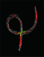
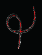
Figure 3: The binary image of the point cloud (in white) from the rope and the linearization of the intersection points: (a) The pixels (in red) obtained by the dilation and thinning of the binary image, and the intersection points (in green); (b) The pixels linearized by the Bresenham algorithm.

3.1 Split Step

The first step of the split and merge method is to divide the obtained point cloud into smaller segments, as shown in Algorithm 1. First, an EMST is constructed based on the points. The EMST is an acyclic edge-weighted graph $T=(\mathcal{V},\mathcal{E})$, where $\mathcal{V}$ is the vertices set and $\mathcal{E}$ is the set of the edges connecting every two vertices $\mathbf{v}_{i},\mathbf{v}_{j}\in\mathcal{V}$ and $i\neq j$. The weight of the edge is defined as the Euclidean distance of the two vertices $\epsilon=\left\|\mathbf{v}_{i}-\mathbf{v}_{j}\right\|$ lee2000curve ; sedgewick2011algorithms . The EMST is constructed by selecting the set of connected edges to ensure the summation of the weights of the edges is minimum. The Prim’s algorithm is used to generate the EMST sedgewick2011algorithms .

After the construction of the EMST, the longest path of the EMST is found by two breadth first searches (BFS) sedgewick2011algorithms . The first BFS is used to traverse the EMST with a random chosen vertex from the EMST, and the path with the largest weight and one end point of the longest path are found. Then, another BFS traverses the EMST, starting with the end point that was found in the prior iteration. The longest path $P=(\mathcal{V}_{p},\mathcal{E}_{p})$ is found which is also the longest path of the EMST $T=(\mathcal{V},\mathcal{E})$, where $\mathcal{V}_{p}\subset\mathcal{V}$ and $\mathcal{E}_{p}\subset\mathcal{E}$. The orange line segments shown in Fig. 2 (b) are the longest path of the EMST $T=(\mathcal{V},\mathcal{E})$.

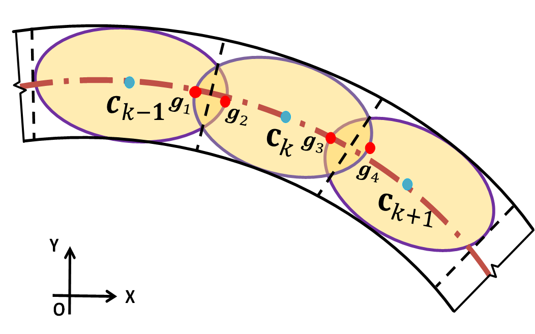
Figure 4: Adjustment of the ellipses with overlaps.

Set the threshold $\gamma$;

Obtain the point cloud $\mathbf{Z}=\{\mathbf{z}_{r}\}_{r=1}^{N_{r}}$;

Build the EMST $T=(\mathcal{V},\mathcal{E})$;

Find the longest path of the EMST $P=(\mathcal{V}_{p},\mathcal{E}_{p})$ by BFSs;

Delete $\mathcal{E}_{p}$, then there are many small clusters (trees) $\mathcal{C}=\left\{\mathcal{C}_{h}\right\}_{h=1}^{J_{h}}$;

Initialize empty sets $\mathcal{A}$ and $\mathcal{B}$;

Initialize $h=1$;

while  $h\leq J_{h}$  do

      

      Calculate $D_{h}$ in (17);

      

      if  $D_{h}>\gamma$ then

            

            Append $\mathcal{C}_{h}$ to $\mathcal{A}$;

       end if

      

      else

            $\mathcal{B}=\mathcal{B}\cup\mathcal{C}_{h}$;

       end if

      

      $h=h+1$;

end while

Append $\mathcal{B}$ to $\mathcal{A}$;

Algorithm 1 The segmentation of the elongated deformable object

After the construction of the EMST and the longest path $P=(\mathcal{V}_{p},\mathcal{E}_{p})$ is found, the EMST is segmented into smaller disconnected clusters (or trees) by deleting the $\mathcal{E}_{p}$ from the EMST $T$. Then, there are some small trees $\mathcal{C}=\left\{\mathcal{C}_{h}\right\}_{h=1}^{J_{h}}$ left. The distance $D_{h}$ between $\mathcal{C}_{h}$ and $\mathcal{V}_{p}$ is defined as

$$D_{h}=\textrm{sup}\left\{\textrm{inf}\{\left\|\mathbf{u}_{i}-\mathbf{v}_{j}\right\||\forall\mathbf{v}_{j}\in\mathcal{V}_{p}\}|\forall\mathbf{u}_{i}\in\mathcal{C}_{h}\right\}$$ (17)

where $\mathbf{v}_{j}$ are vertices from $\mathcal{V}_{p}$ and $\mathbf{u}_{i}$ are vertices from $\mathcal{C}_{h}$. If $D_{h}$ is larger than a predefined threshold $\gamma$, the cluster $\mathcal{C}_{h}$ and the $\mathcal{V}_{p}$ are from different regions of the rope, instead of the small branches of the $P$. After the $O_{n}$ different parts (or smaller clusters) of the rope $\mathcal{A}=\{\mathcal{A}_{n}\}_{n=1}^{O_{n}}$ are found, the common vertices $\mathcal{V}_{C}=\{\mathbf{v}_{c}|\mathbf{v}_{c}\in\mathcal{A}\backslash\mathcal{B},\mathbf{v}_{c}\in\mathcal{V}_{P},c=1,\cdots,O_{n}-1\}$ of the $O_{n}$ clusters are also found, where the points of $\mathcal{B}$ are from the same region of the rope as $\mathcal{V}_{P}$. The common vertices have more than $2$ edges connected with them. If the distance between some common vertices are smaller than the predefined threshold $\gamma$, their mean values are used to represent them. The EMST is segmented into $O_{n}=2$ clusters (orange and blue line segments) shown in Fig. 2 (b).

Each cluster is an EMST and the longest path with two end points are found by two BFSs. Starting with one end point, the cluster is divided into $M_{n}$ smaller segments $\mathcal{S}_{n}=\{\mathcal{S}_{u,n}\}_{u=1}^{M_{n}}\subset\mathcal{A}_{n}$, with each segment $\mathcal{S}_{u,n}$ satisfying

$$\textrm{sup}\{\left\|\mathbf{z}_{i}-\mathbf{z}_{j}\right\||\forall\mathbf{z}_{i},\mathbf{z}_{j}\in\mathcal{S}_{u,n},i\neq j\}\leq H$$ (18)

where $H$ is a predefined parameter and $\mathbf{z}$ is the point inside the smaller segments $\mathcal{S}_{u,n}$. The center of each segment $\mathbf{c}_{u,n}$ is calculated as

$$\mathbf{c}_{u,n}=\frac{1}{L_{u,n}}\sum_{i=1}^{L_{u,n}}\mathbf{z}_{i},\mathbf{z}_{i}\in\mathcal{S}_{u,n}$$ (19)

where $L_{u,n}$ is the number of points in segment $\mathcal{S}_{u,n}$. The segments are shown with different colors and the red points are the centers of the segments in Fig. 2 (c).

Set the distance $H$;

Given the $O_{n}$ clusters $\mathcal{A}=\{\mathcal{A}_{n}\}_{n=1}^{O_{n}}$;

Given the common vertices $\mathcal{V}_{C}=\{\mathbf{v}_{c}|\mathbf{v}_{c}\in\mathcal{\mathcal{A}\backslash\mathcal{B}},\mathbf{v}_{c}\in\mathcal{V}_{p},c=1,\cdots,O_{n}-1\}$;

Initialize $n,c=1$;

while $n\leq O_{n}$  do

      

      Divide $\mathcal{A}_{n}$ into smaller segments $\mathcal{S}_{n}=\{\mathcal{S}_{u,n}\}_{u=1}^{M_{n}}$ satisfies (18);

      

      Calculate $\mathbf{c}_{u,n}$ in (19);

      

      Create the graph $T_{m}=(\mathcal{V}_{m},\mathcal{E}_{m})$ with $\mathbf{c}_{u,n}\in\mathcal{V}_{m}$ and $\{\mathbf{c}_{u,n},\mathbf{c}_{u+1,n}\}\in\mathcal{E}_{m}$ and $u=1,\cdots,M_{n}-1$;

      

      $n=n+1$;

end while

while $c\leq O_{n}-1$  do

      

      Find the centers $\mathcal{Q}=\{\mathbf{c}_{q}\}_{q=1}^{4}\subset\mathcal{V}_{m}$ closest to $\mathbf{v}_{c}$, and delete edges between them;

      

      Calculate vectors $\mathbf{d}_{q}$;

      

      Find the two pairs $(i^{*},j^{*})$, based on (20);

      

      Create the edges $e$;

      

      $\mathcal{E}_{m}=\mathcal{E}_{m}\cup e$;

      

      $\mathcal{V}_{m}=\mathcal{V}_{m}\cup\mathbf{v}_{c}$;

      

      $c=c+1$;

end while

Complete the graph $T_{m}=(\mathcal{V}_{m},\mathcal{E}_{m})$;

Fit B-spline by the ordered centers and readjust the centers;

Algorithm 2 The ordering of the centers and B-spline interpolation

3.2 Merge Step

Previously the elongated target is subdivided into small segments and the centers of the segments are found. In this step, the order information of the centers is generated and a B-spline curve is traced, which represents the global shape and configuration information of the target as shown in Algorithm 2. At first, a graph $T_{m}=(\mathcal{V}_{m},\mathcal{E}_{m})$ is created, such that the center of each segment constitutes the vertex $\mathbf{c}_{u,n}\in\mathcal{V}_{m}$ and the edges are built by connecting the centers of nearby segments in each cluster $\mathcal{A}_{n}$ as $\{\mathbf{c}_{u,n},\mathbf{c}_{u+1,n}\}\in\mathcal{E}_{m}$ and $u=1,\cdots,M_{n}-1$.

For the common vertex $\mathbf{v}_{c}\in\mathcal{V}_{C}$, the closest four centers are found $\mathcal{Q}=\{\mathbf{c}_{q}\}_{q=1}^{4}\subset\mathcal{V}_{m}$. The edges between these four centers are deleted and the new edges between them are found in the following way. The vectors $\mathbf{d}_{q}=\frac{\mathbf{v}_{c}-\mathbf{c}_{q}}{\left\|\mathbf{v}_{c}-\mathbf{c}_{q}\right\|}$ are calculated, and the pair $(i^{*},j^{*})$ is found that meets

$$\textrm{$\underset{\mathit{i,j\in q,i\neq j}}{\mathrm{arg\,}\min}$}\left\|\mathbf{d}_{i}+\mathbf{d}_{j}\right\|$$ (20)

The vertex $\mathbf{v}_{c}$ is added to the graph as $\mathcal{V}_{m}=\mathcal{V}_{m}\cup\mathbf{v}_{c}$. Then, the edges are generated as $e_{1}=\{\mathbf{c}_{i^{*}},\mathbf{v}_{c}\}$ and $e_{2}=\{\mathbf{v}_{c},\mathbf{c}_{j^{*}}\}$, which connect between $\mathbf{v}_{c}$ and the two centers $\mathbf{c}_{i^{*}}$ and $\mathbf{c}_{j^{*}}$, giving the minimum value of (20). The edges $e_{1}$ and $e_{2}$ are added to the graph $T_{m}$ as $\mathcal{E}_{m}=\mathcal{E}_{m}\cup e_{1}$ and $\mathcal{E}_{m}=\mathcal{E}_{m}\cup e_{2}$. The $2$ remaining centers are connected as another edge $e_{3}$ and it is added to the graph $T_{m}$ as $\mathcal{E}_{m}=\mathcal{E}_{m}\cup e_{3}$. Finally, the graph $T_{m}=(\mathcal{V}_{m},\mathcal{E}_{m})$ is completed by adding an edge to the $2$ centers of the closest end segments from different clusters to make all the centers ordered.

The initial B-spline curve is interpolated by the ordered centers using (15) and (16). The ellipses may have overlaps as shown in Fig. 4. The centers are adjusted to decrease the overlap between ellipses by using the following formula:

$$\mathbf{c}_{k}=\frac{\left(\mathbf{g}_{1}+\mathbf{g}_{2}\right)+\left(\mathbf{g}_{3}+\mathbf{g}_{4}\right)}{4}$$ (21)

where $\mathbf{c}_{k}$ is the center of the $k\textrm{th}$ ellipse, $\mathbf{g}_{1}$ and $\mathbf{g}_{4}$ are the endpoints of the $k\textrm{th}$ ellipse, $\mathbf{g}_{2}$ is the endpoint of the $\left(k-1\right)\textrm{th}$ ellipse and $\mathbf{g}_{3}$ is the endpoint of the $\left(k+1\right)\textrm{th}$ ellipse. The centers are deleted if their distances to the common vertices are smaller than $H$.

    

    

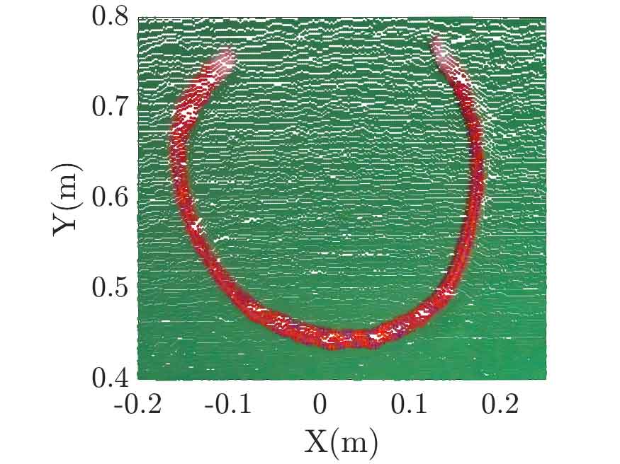
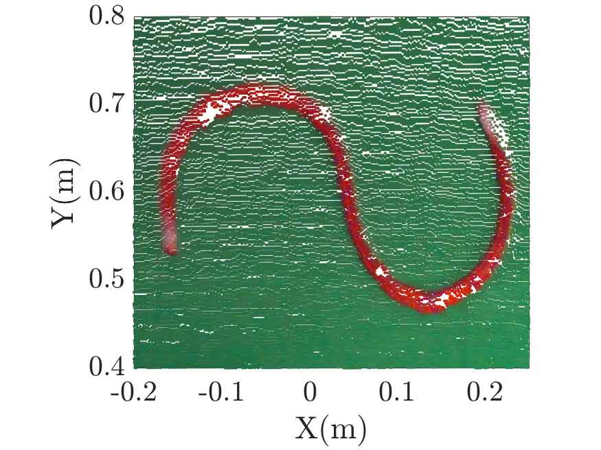
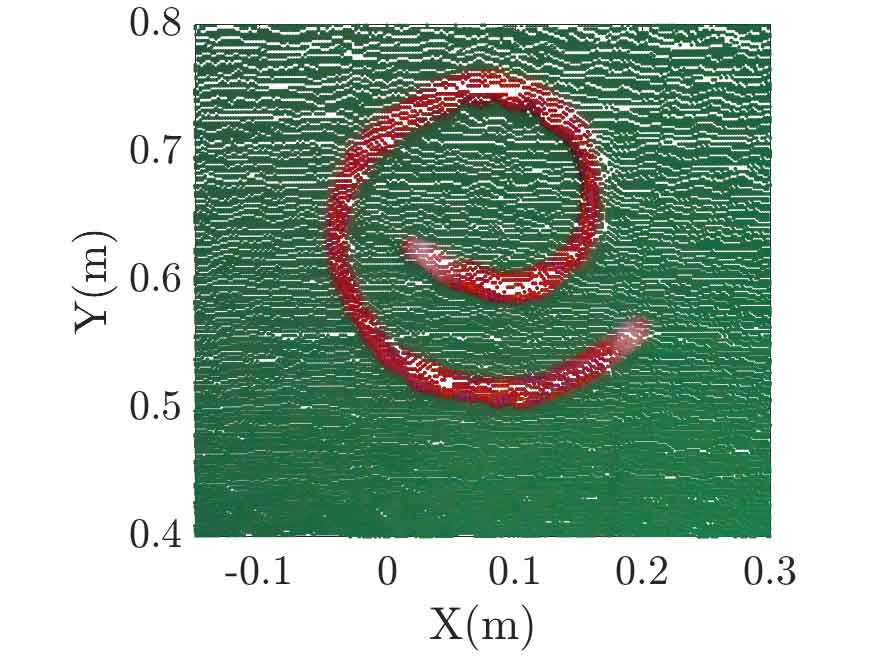
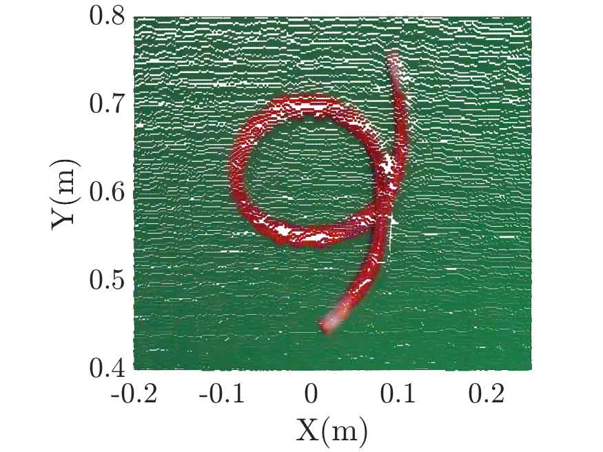
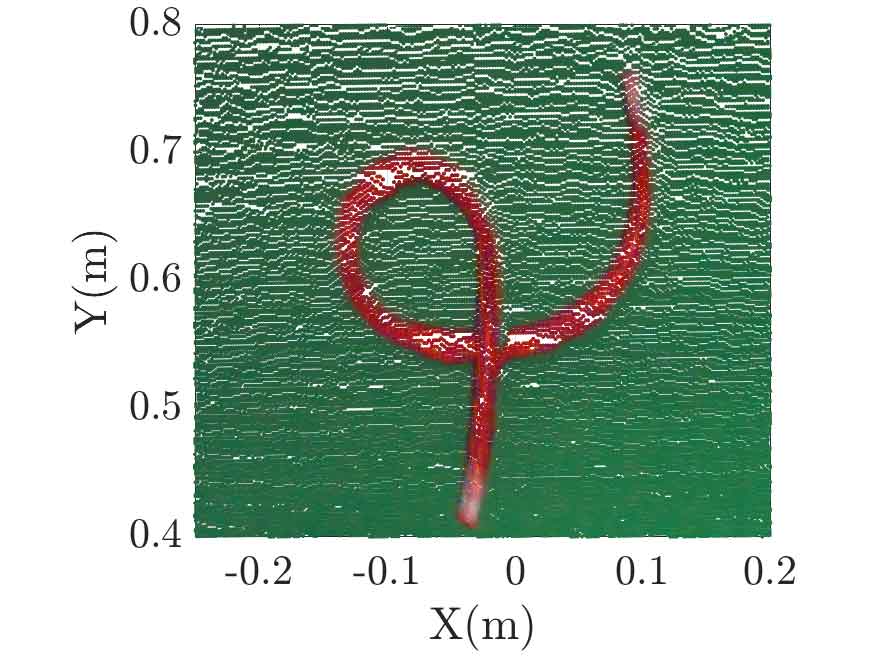
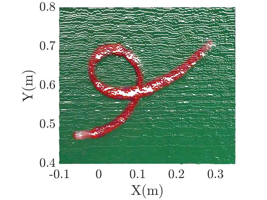
Figure 5: Point clouds of the rope in different configurations obtained from an RGB-D camera.

4 Experimental Results

In order to validate the proposed B-spline chained RMMs, a series of experiments are performed to estimate the shape of the elongated deformable objects. Intersection over union (IoU) is used as the metric to evaluate the accuracy of shape estimation of the proposed algorithm. The IoU is defined as the area of intersection of the estimated shape and the true shape divided by the union of the two shapes zea2016tracking

$$\mathbf{IoU}=\frac{area(\mathbf{\theta^{*}})\cap area(\mathbf{\hat{\theta}})}{area(\mathbf{\theta^{*}})\cup area(\mathbf{\hat{\theta}})}$$ (22)

where $\mathbf{\hat{\theta}}$ is the true shape parameters and $\mathbf{\theta^{*}}$ is the estimated shape parameters. IoU is between $0$ and $1$, where the value $1$ corresponds to a perfect match between the estimated area and the ground-truth. Since the ground-truth of the position and the shape of the elongated deformable object is difficult to obtain, the measurements from the RGB-D camera are used as the ground-truth zea2016tracking . The measurement noise is neglected because it is small compared to the area of the elongated deformable object. The ground-truth is constructed by creating a $1\textrm{px}\times 1\textrm{px}$ rectangle at each measurement point and taking the union of all the rectangles zea2016tracking . The dilation and erosion methods are applied to ensure that the pixels are fully connected while preserving the boundary of the target.

   

   

   

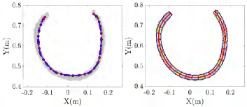
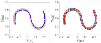
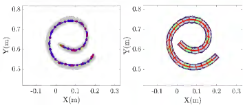
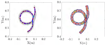
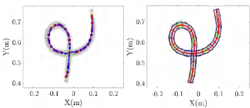
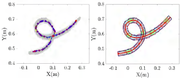
Figure 6: Shape estimation results on the rope in 6 different configurations. For each sub-figure (a)-(f), the left plot is the initialization result and the right plot is the estimated shape of the rope.

4.1 Shape Estimation Results of The Static Rope

A red nylon dock line with width of $15.8\textrm{mm}$ and length of $930\textrm{mm}$ is used in the first part of the experiment. The rope is manipulated to $6$ different shapes either with or without intersection. A green cloth is used as the background. A Microsoft^® Kinect camera is used to obtain a point cloud of the rope. Plane fitting method and clustering algorithms are applied to subtract the rope point cloud from the background. The point clouds of the rope with $6$ different configurations are shown in Fig. 5.

The shape estimation results on $6$ different configurations of the rope are shown in Fig. 6. Each sub-figure includes two plots. The left plot is the initialization result. The gray measurement points are the measurements from the rope. The colored segments are the initial segments. The red dots are the centers of each segment and the blue line segments are the initial graph of the centers. The right plot is the estimated shape of the rope. The segmented measurement points are denoted by different colors. The red ellipses represent multiple RMMs and the red curve is the B-spline curve of the centers of the ellipses. The offset curves in blue in Fig 6 are created by shifting the estimated B-spline curve by half of the estimated width of the rope. The $H$ value in (18) in the initialization procedure is set to $30\textrm{mm}$. The degree of the B-spline curve is set to $2$ and the number of the control points is set to $13$ for all 6 configurations. The maximum iteration number of the EM algorithm is set to $3$.

Table 1: The estimated width and IoU values of the rope in $6$ different configurations.

Configuration	1	2	3	4	5	6
Width (mm)	11.4	11.2	13.7	13.0	12.3	14.9
IoU	0.752	0.738	0.731	0.732	0.736	0.715
IoUschulman2013tracking	0.683	0.654	0.632	0.603	0.642	0.520

The estimated width of the rope and the IoU values are shown in Table 1. The estimated width is smaller than the true width (15.8mm) and the average IoU value over 6 configurations is $0.734$. Because the surface of the rope is not flat, the detection of the edge points of the rope using Kinect sensor is hard. This causes the estimates of the width of the rope to be smaller than the ground-truth. Algorithm in schulman2013tracking is also applied to estimate the shape of the rope in $6$ configurations, of which the code is publicly available (http://rll.berkeley.edu/tracking/). The algorithm in schulman2013tracking models a virtual rope as a set of serial-linked capsules in a simulation. The radius of the capsules is set as 7.9mm and other parameters are set to the default settings. The shape estimations of the proposed algorithm are more accurate compared with the algorithm in schulman2013tracking , based on the IoU values shown in Table 1.

The experiments are performed by measuring the elongated deformable object on a tabletop with an RGB-D sensor. The sensor only detects the top surface of the elongated deformable object closest to the sensor. Thus, the two dimensional shape is estimated by the proposed algorithm and the third dimension is determined by the tabletop. However, the proposed model can be extended to estimate the shape of the rope in three dimensional space. The control points of the B-spline curve in (1) can be extended into three dimensions as $\mathbf{b}_{i}\in\mathbb{R}^{3\times 1}$ de1978practical . RMM can also be extended into three dimensions to represent an ellipsoid feldmann2011tracking .

Table 2: Typical execution time for initialization and EM algorithms with the rope in $6$ different configurations.

Configuration	1	2	3	4	5	6
Initialization (sec)	0.195	0.196	0.199	0.221	0.212	0.215
EM (sec)	0.296	0.291	0.283	0.253	0.248	0.252

        

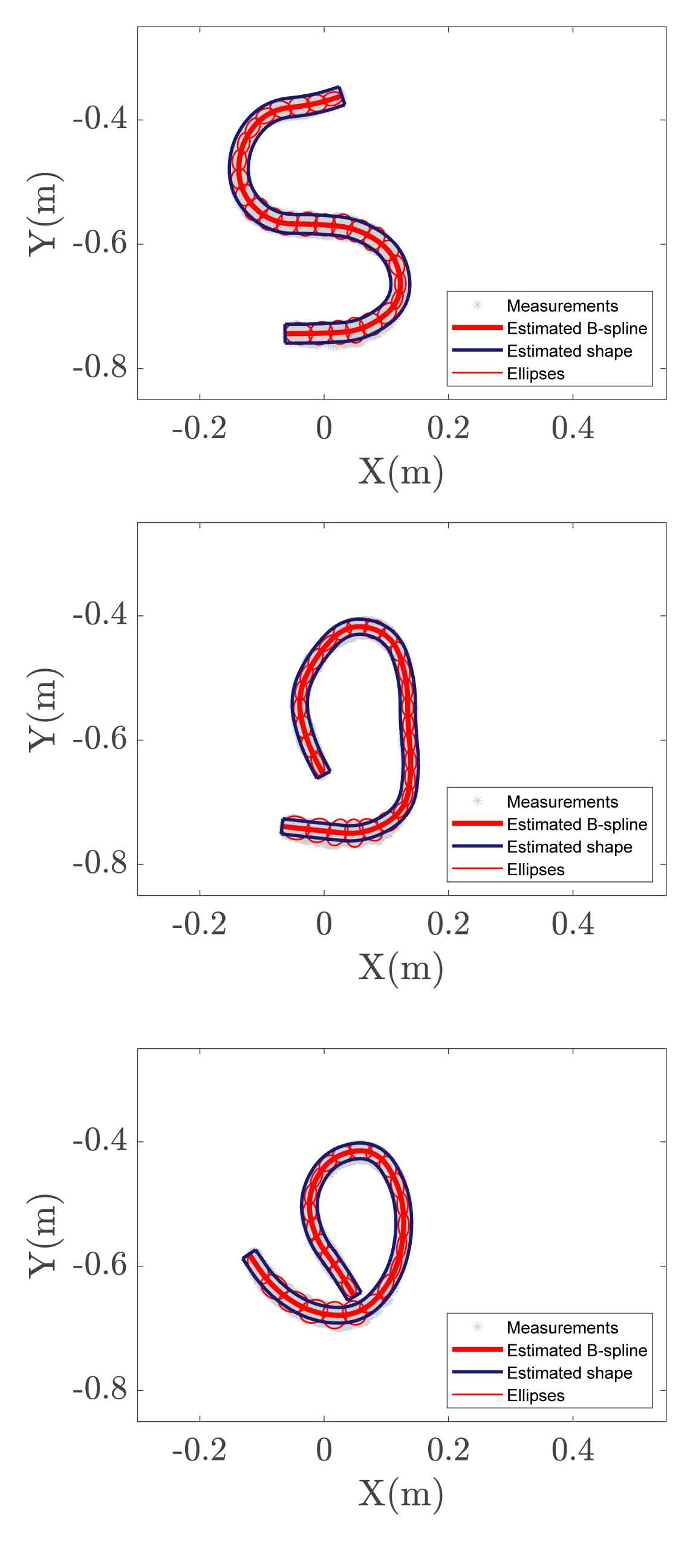
(a) Rope1

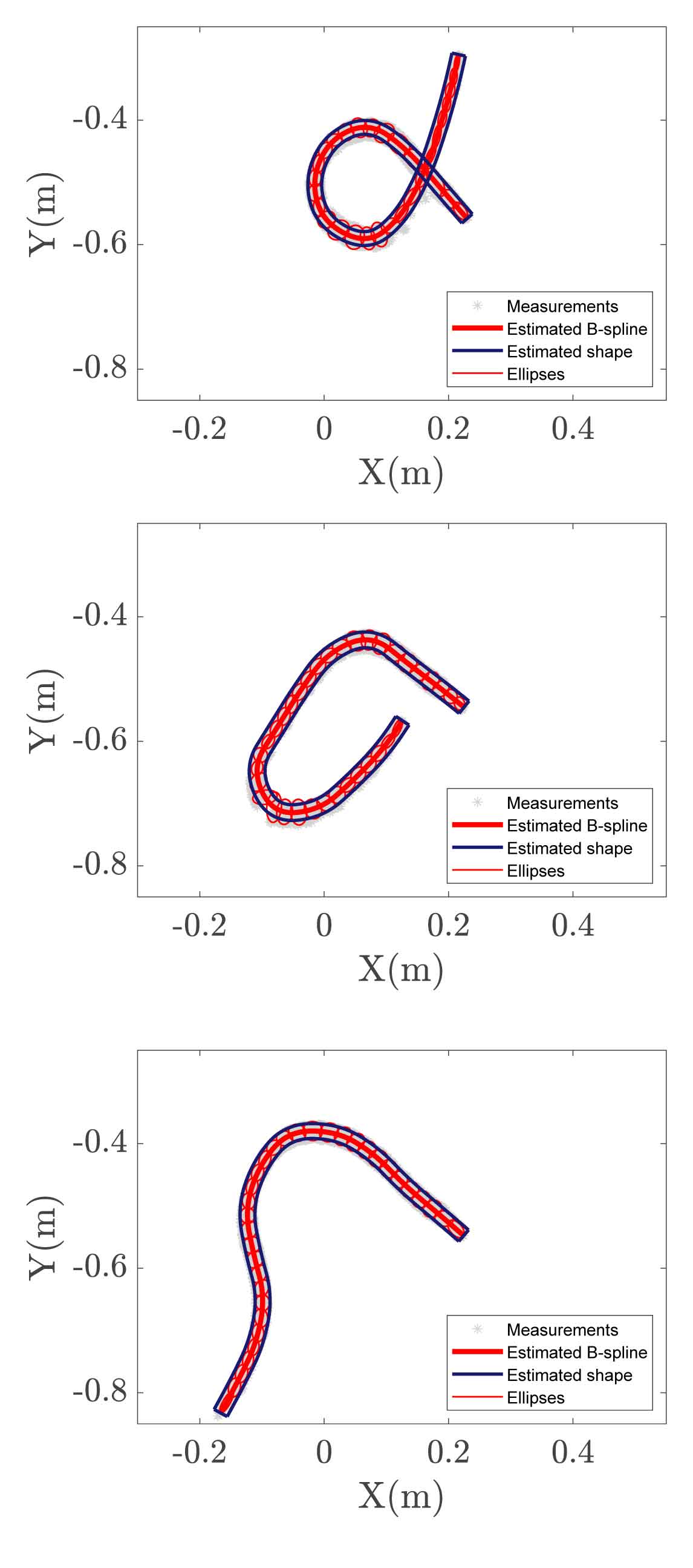
(b) Rope2

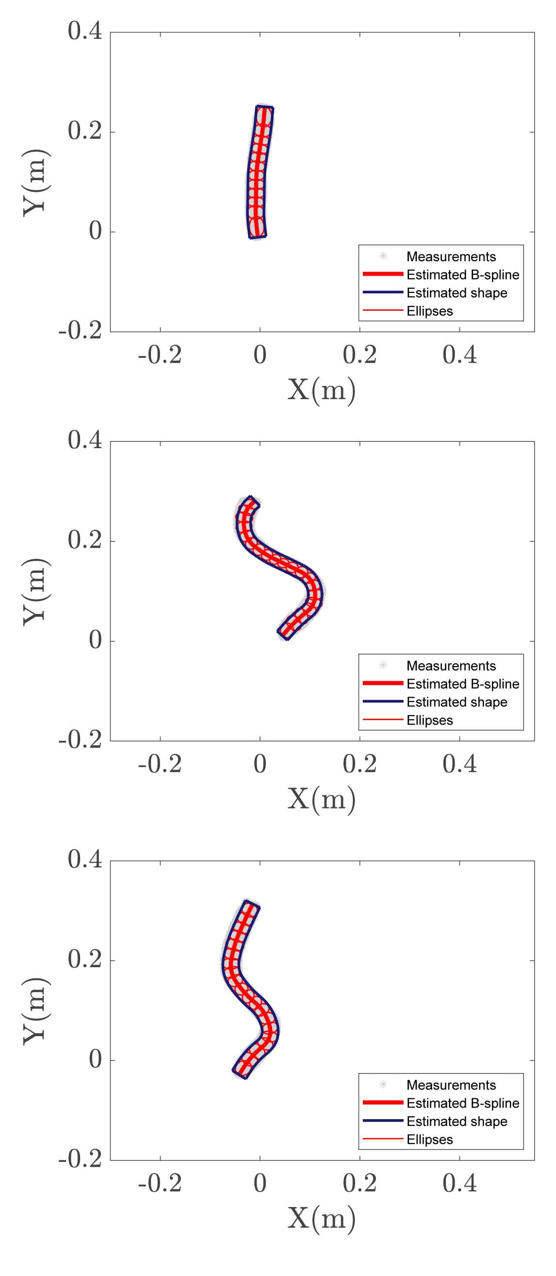
(c) Tube1

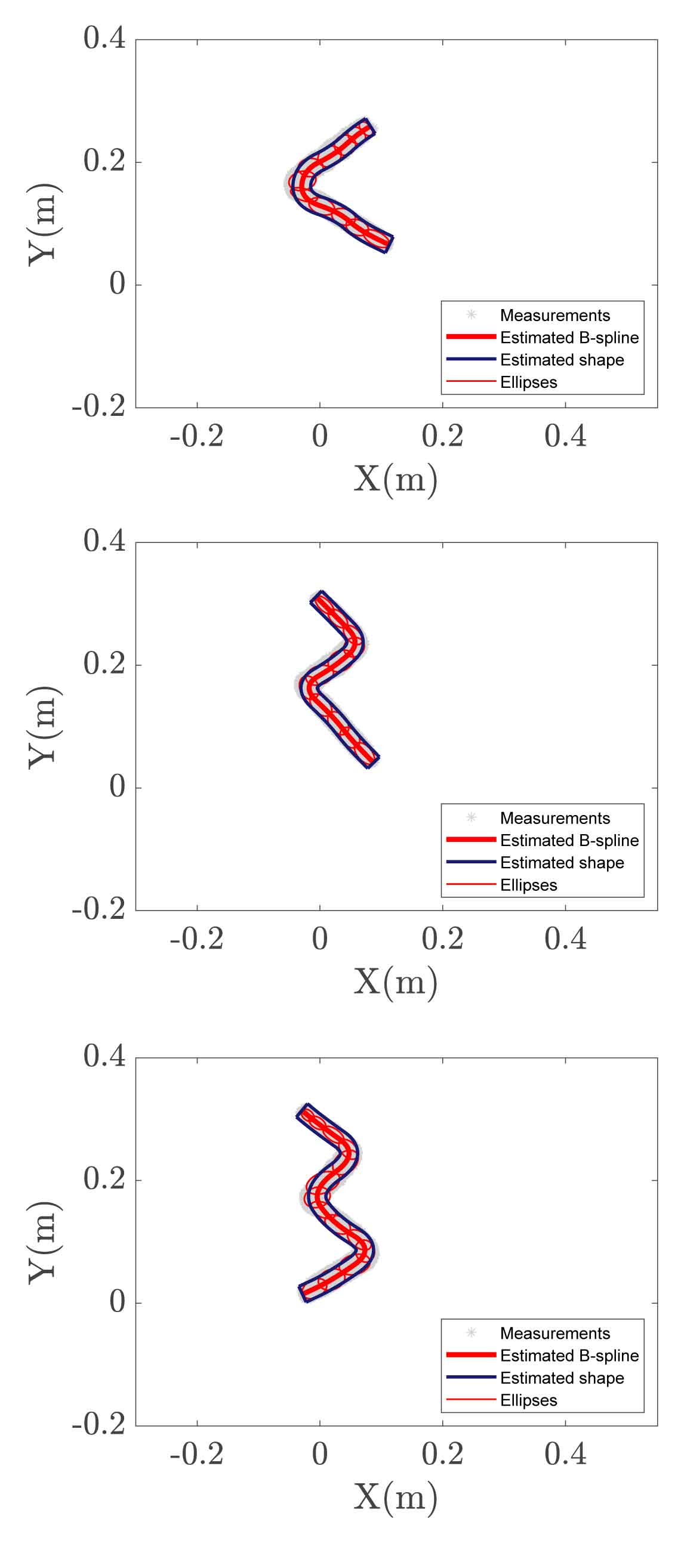
(d) Tube2

(e) Assembling

Figure 7: Shape estimation results on the rope and the plastic tube during manipulations. For each sub-figure (a)-(e), the $1^{st}$ frame, the $25^{th}$ frame and the $50^{th}$ frame are shown from top to bottom.

The codes of the initialization and EM algorithms were run in MATLAB^® R2019b on a Windows 10 PC with Intel^® $\mathrm{i7-9700k@3.60GHZ}$ processor and $\mathrm{32.0GB}$ of RAM. The typical execution time for initialization and EM algorithms are shown in Table 2. The most time consuming parts of the initialization stage are building the EMST and the calculation of the distance $D_{h}$ in (17). The time complexity of building the EMST is $\mathcal{O}(\left|\mathrm{\mathcal{E}}\right|\mathrm{log}\left|\mathcal{V}\right|)$, where $\left|\mathrm{\mathcal{E}}\right|$ and $\left|\mathcal{V}\right|$ are the number of edges and vertices in graph $T=(\mathcal{V},\mathcal{E})$ sedgewick2011algorithms . The calculation of distance $D_{h}$ in (17) requires $\mathcal{O}(\left|\mathcal{V}_{p}\right|\left|\mathcal{C}_{h}\right|)$ operations, where $\left|\mathcal{V}_{p}\right|$ is the number of vertices from $\mathcal{V}_{p}$ and $\left|\mathcal{C}_{h}\right|$ is the number of vertices from $\mathcal{C}_{h}$. The time complexity of the EM algorithm is determined by the expectation stage, which assigns the measurements into different ellipses. The time complexity is $\mathcal{O}(KN_{r}),$ where $N_{r}$ is the number of the measurements $\mathbf{Z}=\{\mathbf{z}_{r}\}_{r=1}^{N_{r}}$ and $K$ is the number of clusters. In order to reduce the execution time for the shape estimation of the elongated deformable object, parallel computing can be used or the number of measurements can be uniformly down sampled.

Table 3: The average execution times and average IoU values of the rope and the plastic tube during manipulations.

Video name	Rope1	Rope2	Tube1	Tube2	Assembling
shape change	$\surd$	$\surd$	$\surd$	$\surd$	$\surd$
length change			$\surd$	$\surd$	$\surd$
execution time (sec/frame)	0.343	0.422	0.450	0.445	0.441
IoU	0.727	0.709	0.799	0.768	0.819

4.2 Shape Estimation Results During Manipulations and Assembly

The previous experiments show the shape estimation of the rope in $6$ different configurations, based on the measurements from one frame. The proposed EM algorithm is also used for shape estimation of the elongated deformable object over multiple frames. The IoU value between the estimated shape of the previous time step and the current measurements is calculated for each frame. If the calculated IoU value is smaller than a threshold, the initialization procedure is rerun in consideration of the abrupt changes of the shape or the length of the elongated object.

Besides the red nylon dock line, a flexible red plastic tube with modifiable shape and length is also used in the experiments. The elongated deformable objects are manipulated in $5$ different scenarios. The scenarios and the estimated results are recorded as videos (see the multimedia attachment). Each video has $50$ frames of point cloud measurements. The video ‘Rope1’ shows the scenario that the rope is manipulated from the shape ‘s’ to the shape ‘9’. The video ‘Rope2’ demonstrates the scenario when the rope changes from one intersection configuration to non-intersection configuration. The ‘Tube1’ shows that the plastic tube is stretched and squeezed which changes both the shape and the length. The video ‘Tube2’ illustrates that one part of the plastic tube is stretched at a time and the red plastic tube is manipulated from the shape ‘L’ to the shape ‘M’. The last video ‘Assembling’ shows the situation when two plastic tubes are assembled together as one tube.

The typical frames and the estimation results are shown in Fig. 7. The description of the videos and the estimation results, including the average IoU value and the average execution time over $50$ frames for each video, are shown in Table. 3. Algorithm in schulman2013tracking is applied to estimate the shape of the rope in ‘Rope1’ and ‘Rope2’ scenarios. The average IoU values for ‘Rope1’ and ‘Rope2’ scenarios are $0.505$ and $0.608$ separately. The proposed algorithm achieves better accuracy in terms of IoU. Because the Algorithm in schulman2013tracking uses linked rigid objects as the simulation model of the rope, it cannot work for the scenarios (e.g. ‘Tube1’, ‘Tube2’ and ‘Assembling’) when the elongated object are changing both length and shape during the manipulations.

5 Conclusions and Future Work

To localize the elongated deformable object and to estimate its shape, a B-spline chained multiple RMMs representation and its corresponding EM algorithm are developed in this paper. Based on the sparse measurements from an RGB-D camera, the proposed algorithm approximates the elongated deformable object as a set of chained ellipses by using a B-spline curve. Each ellipse is represented by an RMM, of which the center represents the location and the covariance matrix determines the shape of the ellipse. All the centers are enforced to be located on a B-spline curve, which represents the shape of the elongated deformable object. The EM algorithm and its initialization method are presented to estimate the control points of the B-spline curve as well as the RMMs. The performance of the proposed shape estimation algorithm is evaluated using real measurements of a red dock line in 6 different configurations. The proposed algorithm is also used to estimate the shapes in scenarios such as the continuous manipulation and the assembly of elongated deformable objects. From the experimental results, it can be concluded that the B-spline curve chained RMM algorithm is capable of estimating the shape of the elongated deformable object configured as intersecting and non-intersecting shapes. The case when the rope has more than one intersection, has knots or is piled up will be studied in the future work.

References

- (1) A. Shah, L. Blumberg, and J. Shah, “Planning for manipulation of interlinked deformable linear objects with applications to aircraft assembly,” IEEE Transactions on Automation Science and Engineering, no. 99, pp. 1–16, 2018.
- (2) A. Zea, F. Faion, and U. D. Hanebeck, “Tracking elongated extended objects using splines,” in 19th International Conference on Information Fusion (FUSION), 2016, pp. 612–619.
- (3) J. Sanchez, J.-A. Corrales, B.-C. Bouzgarrou, and Y. Mezouar, “Robotic manipulation and sensing of deformable objects in domestic and industrial applications: a survey,” The International Journal of Robotics Research, vol. 37, no. 7, pp. 688–716, 2018.
- (4) R. C. Jackson, R. Yuan, D.-L. Chow, W. S. Newman, and M. C. Çavuşoğlu, “Real-time visual tracking of dynamic surgical suture threads,” IEEE Transactions on Automation science and Engineering, vol. 15, no. 3, pp. 1078–1090, 2017.
- (5) T. Tang and M. Tomizuka, “Track deformable objects from point clouds with structure preserved registration,” The International Journal of Robotics Research, 2018.
- (6) J. Schulman, A. Lee, J. Ho, and P. Abbeel, “Tracking deformable objects with point clouds,” in IEEE International Conference on Robotics and Automation (ICRA), 2013, pp. 1130–1137.
- (7) A. Petit, V. Lippiello, and B. Siciliano, “Real-time tracking of 3d elastic objects with an RGB-D sensor,” in IEEE/RSJ International Conference on Intelligent Robots and Systems (IROS), 2015, pp. 3914–3921.
- (8) S. Javdani, S. Tandon, J. Tang, J. F. O’Brien, and P. Abbeel, “Modeling and perception of deformable one-dimensional objects,” in IEEE International Conference on Robotics and Automation (ICRA), 2011, pp. 1607–1614.
- (9) D. De Gregorio, G. Palli, and L. Di Stefano, “Let’s take a walk on superpixels graphs: Deformable linear objects segmentation and model estimation,” in Asian Conference on Computer Vision (ACCV), 2018, pp. 662–677.
- (10) W. H. Lui and A. Saxena, “Tangled: Learning to untangle ropes with rgb-d perception,” in IEEE/RSJ International Conference on Intelligent Robots and Systems (IROS), 2013, pp. 837–844.
- (11) T. Matsuno and T. Fukuda, “Manipulation of flexible rope using topological model based on sensor information,” in IEEE/RSJ International Conference on Intelligent Robots and Systems (IROS), 2006, pp. 2638–2643.
- (12) G. Yao and A. Dani, “Image moment-based random hypersurface model for extended object tracking,” in 20th International Conference on Information Fusion (Fusion), 2017, pp. 1–7.
- (13) G. Yao, K. Hunte, and A. Dani, “Image moment-based object tracking and shape estimation for complex motions,” in American Control Conference (ACC), 2018, pp. 5819–5824.
- (14) M. Feldmann, D. Franken, and W. Koch, “Tracking of extended objects and group targets using random matrices,” IEEE Transactions on Signal Processing, vol. 59, no. 4, pp. 1409–1420, 2011.
- (15) C. De Boor, C. De Boor, E.-U. Mathématicien, C. De Boor, and C. De Boor, A practical guide to splines. springer-verlag New York, 1978, vol. 27.
- (16) E. T. Lee, “Choosing nodes in parametric curve interpolation,” Computer-Aided Design, vol. 21, no. 6, pp. 363–370, 1989.
- (17) C. M. Bishop, Pattern recognition and machine learning. springer, 2006.
- (18) H. Huang, S. Wu, D. Cohen-Or, M. Gong, H. Zhang, G. Li, and B. Chen, “L1-medial skeleton of point cloud.” ACM Trans. Graph., vol. 32, no. 4, pp. 65–1, 2013.
- (19) I.-K. Lee, “Curve reconstruction from unorganized points,” Computer aided geometric design, vol. 17, no. 2, pp. 161–177, 2000.
- (20) R. Sedgewick and K. Wayne, Algorithms. Addison-Wesley Professional, 2011.