TUM-HEP 1256/20

Lessons from eclectic flavor symmetries

Hans Peter Nilles^a, Saúl Ramos–Sánchez^b,c, Patrick K.S. Vaudrevange^c

^aBethe Center for Theoretical Physics and Physikalisches Institut der Universität Bonn,
Nussallee 12, 53115 Bonn, Germany

^bInstituto de Física, Universidad Nacional Autónoma de México,
POB 20-364, Cd.Mx. 01000, México

^cPhysik Department T75, Technische Universität München,
James-Franck-Straße 1, 85748 Garching, Germany

A top-down approach to the flavor problem motivated from string theory leads to the concept of eclectic flavor groups that combine traditional and modular flavor symmetries. To make contact with models constructed in the bottom-up approach, we analyze a specific example based on the eclectic flavor group $\Omega(1)$ (a nontrivial combination of the traditional flavor group $\Delta(54)$ and the finite modular group $T^{\prime}$) in order to extract general lessons from the eclectic scheme. We observe that this scheme is highly predictive since it severely restricts the possible group representations and modular weights of matter fields. Thereby, it controls the structure of the Kähler potential and the superpotential, which we discuss explicitly. In particular, both Kähler potential and superpotential are shown to transform nontrivially, but combine to an invariant action. Finally, we find that discrete $R$-symmetries are intrinsic to eclectic flavor groups.

1 Introduction

We elaborate on a new approach to the flavor problem that combines traditional (discrete) flavor symmetries with modular flavor symmetries. This approach originated in top-down model building motivated by string theory. It has been developed in a series of papers [1, 2, 3], culminating in the concept of eclectic flavor groups [3]. The eclectic flavor group is a maximal extension of the traditional flavor group by (finite) discrete modular symmetries. It allows a new approach to the flavor problem compared to previous attempts that rely separately either on the traditional flavor symmetry or the modular flavor symmetry.

Although discrete flavor symmetries (traditional or modular) are natural ingredients in string theory, not many explicit models have been constructed yet in a top-down (TD) approach. Models with modular symmetries have been constructed in heterotic orbifolds, magnetized branes and intersecting D-brane models [4, 5, 6, 7]. In particular, several promising models have been found with different orbifold geometries [8, 9, 10, 11, 12, 13, 14, 15, 16]. Even in the absence of a large number of explicit and fully satisfactory models, we think that it is time to combine the TD-approach with existing bottom-up (BU) models that exhibit successful fits to masses and mixing angles of quarks and leptons. Our analysis will clarify several conceptional and technical considerations that have not yet been fully addressed in the available literature, such as the need for the consideration of the eclectic extension and a new link between representations and modular weights. To illustrate these questions, we shall use a scheme based on the $\mathbb{T}^{2}/\mathbbm{Z}_{3}$ orbifold which appears, for example, in models based on the $\mathbb{T}^{6}/\mathbbm{Z}_{3}\times\mathbbm{Z}_{3}$ orbifold discussed in ref. [15]. It exhibits the traditional flavor symmetry $\Delta(54)$, the finite modular flavor group $T^{\prime}\cong[24,3]$ and the resulting eclectic flavor group $\Omega(1)\cong[648,533]$ (according to the classification of the computer program GAP [17], where the first number gives the order of the group).

There is still a gap between available TD and BU constructions [18, 19, 20] and there are some questions to be addressed when one tries to explicitly combine them. In BU constructions one freely assumes a certain modular flavor group (like $\Gamma_{N}\cong S_{3},A_{4},S_{4},A_{5}$) as well as all the nontrivial modular weights and representations of these groups (like triplets and nontrivial singlets) that are needed to provide a successful fit to the data [21, 22, 23, 24, 25, 26, 27, 28, 29, 30, 31, 32, 33, 34, 35, 36, 37, 38, 39, 40, 41, 42, 43, 44, 45, 46, 47, 48, 49, 50, 51, 52, 53, 54] following the influential work of Feruglio [20]. In the cases discussed so far there does not yet exist a TD-model that matches all these ingredients (in particular the appearance of all the nontrivial representations).
Our TD example based on the eclectic flavor group $\Omega(1)$ is the one that comes closest to it. This model is suitable to illustrate the following lessons learned from the TD perspective:

• the representations and modular weights of the fields that appear in the low energy effective field theory are highly constrained,

• the eclectic flavor group is more predictive than the traditional flavor group or the finite modular group alone: it severely restricts the superpotential and the Kähler potential,

• discrete $R$-symmetries are naturally related to the eclectic flavor group.

Once these lessons are taken into account, a meaningful link between TU and BU models can be discussed.

The paper is structured as follows: in section 2 we shall present the $\Omega(1)$ model in detail and identify the modular weights and representations of the fields that appear in the massless sector of explicit MSSM-like string models. We emphasize the possibility of having fields with fractional modular weights and discuss how modular weights affect the traditional flavor symmetry. The results are summarized in table 1. Section 3 is devoted to the discussion of the effective action of the $\mathbb{T}^{2}/\mathbbm{Z}_{3}$ orbifold sector, including the superpotential and the Kähler potential. Both of them transform nontrivially under the modular transformation (but combine to a modular invariant action). We shall separately discuss the restrictions based on $T^{\prime}$ and $\Delta(54)$, and illustrate the relevance of both for the eclectic picture. Finally, conclusions and outlook will be given in section 4.

2 Spectrum and symmetries

We focus on symmetric Abelian toroidal orbifold compactifications of the heterotic string [55, 56, 57] that yield both, a $T^{\prime}$ finite modular symmetry and a $\Delta(54)$ traditional flavor symmetry. As derived in refs. [58, 59], a $\Delta(54)$ traditional flavor symmetry appears in compactifications endowed with a $\mathbbm{T}^{2}/\mathbbm{Z}_{3}$ orbifold sector with trivial Wilson line background fields. Moreover, such a $\mathbbm{T}^{2}/\mathbbm{Z}_{3}$ orbifold sector yields a finite modular symmetry $T^{\prime}\cong\mathrm{SL}(2,3)$ [60, 61, 62]. Importantly, these modular and traditional flavor symmetries do not commute and, hence, combine nontrivially to the so-called eclectic flavor group, $\Omega(1)\cong[648,533]$ in this particular case, as explained in ref. [3]. See also ref. [63, 64] for BU flavor model building based on $\Omega(1)$, and ref. [65] for notation. Examples of six-dimensional orbifolds with such a $\mathbbm{T}^{2}/\mathbbm{Z}_{3}$ sector include orbifolds like $\mathbbm{T}^{6}/\mathbbm{Z}_{6}$-II, $\mathbbm{T}^{6}/\mathbbm{Z}_{3}\times\mathbbm{Z}_{3}$ and $\mathbbm{T}^{6}/\mathbbm{Z}_{3}\times\mathbbm{Z}_{6}$. These orbifolds are known to reproduce some properties of the MSSM when used to compactify the $\mathrm{E}_{8}\times\mathrm{E}_{8}$ heterotic string [66, 15, 16, 67, 68].

Since the relevant flavor symmetries are fully determined by the two-dimensional $\mathbbm{Z}_{3}$ orbifold sector, we can restrict our discussion to this sector. There, the orbifold action is generated by a twist $\theta=\exp(\nicefrac{{2\pi\mathrm{i}}}{{3}})$ using complex coordinates for the torus $\mathbbm{T}^{2}$. This twist defines a $\mathbbm{Z}_{3}$ point group with elements $\{\mathbbm{1},\theta,\theta^{2}\}$. Closed strings on $\mathbbm{T}^{2}/\mathbbm{Z}_{3}$ fall into three categories:
(i) Untwisted strings that are trivially closed, even in uncompactified space, associated with the element $\mathbbm{1}$ of the point group.
(ii) Untwisted winding strings that are also associated with the element $\mathbbm{1}$ of the point group but wind around some torus-directions $e_{1}$, $e_{2}$ of the orbifold. In the model discussed here, the winding modes are typically heavy and therefore not relevant for our analysis.
(iii) Twisted strings, which are closed only due to the action of the twist $\theta$ or $\theta^{2}$.

First of all, in the untwisted sector we find the Kähler modulus $T$ of the $\mathbbm{T}^{2}/\mathbbm{Z}_{3}$ orbifold sector that arises from the metric and the antisymmetric $B$-field of the two-torus $\mathbbm{T}^{2}$. In contrast, the complex structure modulus $U$ is fixed to $U=\exp(\nicefrac{{2\pi\mathrm{i}}}{{3}})$ for a $\mathbbm{T}^{2}/\mathbbm{Z}_{3}$, as is well-known. In addition, there are massless untwisted matter strings in four dimensions that originate from ten-dimensional gauge bosons $A^{M}$, $M=0,\ldots,9$ of $\mathrm{E}_{8}\times\mathrm{E}_{8}$ (or $\mathrm{SO}(32)$). Depending on the internal vector index $M$, we denote the corresponding untwisted (i.e. bulk) matter fields by

$$\Phi_{\text{\tiny$-1$}}\;\;\;\mathrm{if}\;\;\;M~{}=~{}4,5\qquad\mathrm{and}\qquad\Phi_{\text{\tiny 0}}\;\;\;\mathrm{if}\;\;\;M~{}=~{}6,7,8,9\;,$$ (1)

assuming that the $\mathbbm{T}^{2}/\mathbbm{Z}_{3}$ orbifold sector lies in the compactified directions $M=4,5$. Note that, as discussed later in section 2.1, the label $n$ of a matter field $\Phi_{n}$ gives the so-called modular weight under a finite modular transformation.

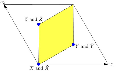
Figure 1: The $\mathbbm{T}^{2}/\mathbbm{Z}_{3}$ orbifold sector: the vectors $e_{1}$ and $e_{2}$ define the two-torus $\mathbbm{T}^{2}$ that exhibits a $\mathbbm{Z}_{3}$ rotational symmetry. The fundamental domain of the $\mathbbm{T}^{2}/\mathbbm{Z}_{3}$ orbifold is depicted as the (yellow) colored region and the three inequivalent fixed points are represented by the (blue) bullets. $(X,Y,Z)^{\mathrm{T}}$ and $(\tilde{X},\tilde{Y},\tilde{Z})^{\mathrm{T}}$ denote localized triplets of matter fields corresponding to twisted strings from the $\theta$ twisted sector without and with oscillator excitations, respectively.

The $\mathbbm{T}^{2}/\mathbbm{Z}_{3}$ orbifold sector has three fixed points, as illustrated in figure 1. At these fixed points, additional massless strings from the $\theta$ and $\theta^{2}$ twisted sectors can be localized. For each twisted sector, there are two classes of massless twisted strings: either with or without oscillator excitations. Consequently, we have two kinds of twisted (i.e. localized) matter fields in the $\theta$ twisted sector. We denote them by

$$\Phi_{\nicefrac{{-2}}{{3}}} = (X,Y,Z)^{\mathrm{T}}\quad\mathrm{without\ oscillator\ excitations}\;,$$ (2a)

$$\Phi_{\nicefrac{{-5}}{{3}}} = (\tilde{X},\tilde{Y},\tilde{Z})^{\mathrm{T}}\quad\mathrm{with\ one\ holomorphic\ oscillator\ excitation}\;,$$ (2b)

respectively, where for example the three matter fields $X$, $Y$ and $Z$ are localized at the three fixed points of the $\mathbbm{T}^{2}/\mathbbm{Z}_{3}$ orbifold sector. We focus in this paper on the couplings of untwisted and $\theta$-twisted matter fields $\Phi_{\text{\tiny 0}}$, $\Phi_{\text{\tiny$-1$}}$, $\Phi_{\nicefrac{{-2}}{{3}}}$ and $\Phi_{\nicefrac{{-5}}{{3}}}$ only. For completeness, let us mention the possible massless anti-triplets of $\theta^{2}$-twisted matter fields, being

$$\Phi_{\nicefrac{{-1}}{{3}}} \quad\mathrm{without\ oscillator\ excitations}\;,$$ (3a)

$$\Phi_{\nicefrac{{+2}}{{3}}} \quad\mathrm{with\ one\ anti}\text{-}\mathrm{holomorphic\ oscillator\ excitation}\;.$$ (3b)

In general, twisted matter fields with further modular weights are possible, but we find that they do not appear in MSSM-like heterotic orbifold compactifications with a $\mathbbm{T}^{2}/\mathbbm{Z}_{3}$ sector possibly due to constraints similar to those presented in ref. [69, table 3]. As a remark, the CPT-partners of the $\theta^{k}$-twisted string states originate from the $\theta^{2k}$ twisted sector for $k=1,2$.

sector	​​matter​​	​​osc.​​	eclectic flavor group $\Omega(1)$
	fields		modular $T^{\prime}$ subgroup				traditional $\Delta(54)$ subgroup
	$\Phi_{n}$		​​irrep $\boldsymbol{s}$​​	$\rho_{\boldsymbol{s}}(\mathrm{S})$	$\rho_{\boldsymbol{s}}(\mathrm{T})$	$n$	​​irrep $\boldsymbol{r}$​​	$\rho_{\boldsymbol{r}}(\mathrm{A})$	$\rho_{\boldsymbol{r}}(\mathrm{B})$	$\rho_{\boldsymbol{r}}(\mathrm{C})$
bulk	$\Phi_{\text{\tiny 0}}$	no	$\boldsymbol{1}$	$1$	$1$	$0$	$\boldsymbol{1}$	$1$	$1$	$+1$
	$\Phi_{\text{\tiny$-1$}}$	no	$\boldsymbol{1}$	$1$	$1$	$-1$	$\boldsymbol{1}^{\prime}$	$1$	$1$	$-1$
$\theta$	$\Phi_{\nicefrac{{-2}}{{3}}}$	no	$\boldsymbol{2}^{\prime}\oplus\boldsymbol{1}$	$\rho(\mathrm{S})$	$\rho(\mathrm{T})$	$\nicefrac{{-2}}{{3}}$	$\boldsymbol{3}_{2}$	$\rho(\mathrm{A})$	$\rho(\mathrm{B})$	$-\rho(\mathrm{C})$
	$\Phi_{\nicefrac{{-5}}{{3}}}$	yes	$\boldsymbol{2}^{\prime}\oplus\boldsymbol{1}$	$\rho(\mathrm{S})$	$\rho(\mathrm{T})$	$\nicefrac{{-5}}{{3}}$	$\boldsymbol{3}_{1}$	$\rho(\mathrm{A})$	$\rho(\mathrm{B})$	$+\rho(\mathrm{C})$
$\theta^{2}$	$\Phi_{\nicefrac{{-1}}{{3}}}$	no	$\boldsymbol{2}^{\prime\prime}\oplus\boldsymbol{1}$	$(\rho(\mathrm{S}))^{*}$	$(\rho(\mathrm{T}))^{*}$	$\nicefrac{{-1}}{{3}}$	$\bar{\boldsymbol{3}}_{1}$	$\rho(\mathrm{A})$	$(\rho(\mathrm{B}))^{*}$	$+\rho(\mathrm{C})$
	$\Phi_{\nicefrac{{+2}}{{3}}}$	yes	$\boldsymbol{2}^{\prime\prime}\oplus\boldsymbol{1}$	$(\rho(\mathrm{S}))^{*}$	$(\rho(\mathrm{T}))^{*}$	$\nicefrac{{+2}}{{3}}$	$\bar{\boldsymbol{3}}_{2}$	$\rho(\mathrm{A})$	$(\rho(\mathrm{B}))^{*}$	$-\rho(\mathrm{C})$
super-	$\mathcal{W}$	-	$\boldsymbol{1}$	$1$	$1$	$-1$	$\boldsymbol{1}^{\prime}$	$1$	$1$	$-1$
​​potential​​

Table 1: $T^{\prime}$ and $\Delta(54)$ irreducible representations of (massless) matter fields $\Phi_{n}$ with modular weights $n$ in MSSM-like heterotic orbifold compactifications with a $\mathbbm{T}^{2}/\mathbbm{Z}_{3}$ sector, see refs. [1, 2] for the derivations. $T^{\prime}$ and $\Delta(54)$ combine nontrivially to the $\Omega(1)\cong[648,533]$ eclectic flavor group [3], generated by $\rho_{\boldsymbol{s}}(\mathrm{S})$, $\rho_{\boldsymbol{s}}(\mathrm{T})$, $\rho_{\boldsymbol{r}}(\mathrm{A})$ and $\rho_{\boldsymbol{r}}(\mathrm{B})$. For $\rho_{\boldsymbol{r}}(\mathrm{C})$, both $\mathrm{C}=\mathrm{S}^{2}$ and the modular weight $n$ are important, as discussed later in eq. (21). Untwisted matter fields $\Phi_{n}$ (with integer modular weights $n$) form one-dimensional representations, while twisted matter fields $\Phi_{n}$ (with fractional modular weights $n$) form (anti-)triplet representations.

2.1 $T^{\prime}$ representations

Let us discuss the modular transformation properties of untwisted and twisted matter fields $\Phi_{n}$ for orbifolds having a $\mathbbm{T}^{2}/\mathbbm{Z}_{3}$ sector.

The modular group $\mathrm{SL}(2,\mathbbm{Z})$ is defined as

$$\gamma~{}=~{}\left(\begin{array}[]{cc}a&b\\ c&d\end{array}\right)~{}\in~{}\mathrm{SL}(2,\mathbbm{Z})\quad\Leftrightarrow\quad ad-bc~{}=~{}1\,\quad\text{ and }\quad a,b,c,d~{}\in~{}\mathbbm{Z}\,.$$ (4)

It can be generated by two elements,

$$\mathrm{S}~{}:=~{}\left(\begin{array}[]{cc}0&1\\ -1&0\end{array}\right)\quad\mathrm{and}\quad\mathrm{T}~{}:=~{}\left(\begin{array}[]{cc}1&1\\ 0&1\end{array}\right)\;,\qquad\mathrm{S},\mathrm{T}~{}\in~{}\mathrm{SL}(2,\mathbbm{Z})\;,$$ (5)

which satisfy the defining relations

$$\mathrm{S}^{4}~{}=~{}(\mathrm{S}\,\mathrm{T})^{3}~{}=~{}\mathbbm{1}\quad\mathrm{and}\quad\mathrm{S}^{2}\,\mathrm{T}~{}=~{}\mathrm{T}\,\mathrm{S}^{2}$$ (6)

of $\mathrm{SL}(2,\mathbbm{Z})$. Under a general modular transformation $\gamma\in\mathrm{SL}(2,\mathbbm{Z})$ from eq. (4), the Kähler modulus $T$ transforms as

$$T~{}\stackrel{{\scriptstyle\gamma}}{{\longrightarrow}}~{}\frac{a\,T+b}{c\,T+d}\;.$$ (7)

Since $T$ transforms identically for $\pm\gamma$, it feels only $\mathrm{PSL}(2,\mathbbm{Z})$ instead of the full $\mathrm{SL}(2,\mathbbm{Z})$ modular group. In contrast, a general matter field $\Phi_{n}$ transforms under $\gamma\in\mathrm{SL}(2,\mathbbm{Z})$ as

$$\Phi_{n}~{}\stackrel{{\scriptstyle\gamma}}{{\longrightarrow}}~{}{\Phi_{n}}^{\prime}~{}:=~{}(c\,T+d)^{n}\,\rho_{\boldsymbol{s}}(\gamma)\,\Phi_{n}\;,$$ (8)

where $(c\,T+d)^{n}$ is the so-called automorphy factor with modular weight $n\in\mathbbm{Q}$. Note that fractional modular weights of both signs are common to string theory, see for example refs. [70, 69]. Moreover, for orbifolds with a $\mathbbm{T}^{2}/\mathbbm{Z}_{3}$ sector, the matrices $\rho_{\boldsymbol{s}}(\gamma)$ build a (reducible or irreducible) representation $\boldsymbol{s}$ of the finite modular group $T^{\prime}\cong\mathrm{SL}(2,3)$, which satisfy the defining relations of $T^{\prime}$,

$$\rho_{\boldsymbol{s}}(\mathrm{S})^{4}~{}=~{}\rho_{\boldsymbol{s}}(\mathrm{T})^{3}~{}=~{}(\rho_{\boldsymbol{s}}(\mathrm{S})\,\rho_{\boldsymbol{s}}(\mathrm{T}))^{3}~{}=~{}\mathbbm{1}\;,\quad(\rho_{\boldsymbol{s}}(\mathrm{S}))^{2}\rho_{\boldsymbol{s}}(\mathrm{T})~{}=~{}\rho_{\boldsymbol{s}}(\mathrm{T})(\rho_{\boldsymbol{s}}(\mathrm{S}))^{2}\;,$$ (9)

cf. eq. (6). In more detail, for the generators $\mathrm{S}$ and $\mathrm{T}$ of $\mathrm{SL}(2,\mathbbm{Z})$, given in eq. (5), a general matter field $\Phi_{n}$ transforms as

$$\Phi_{n} \stackrel{{\scriptstyle\mathrm{S}}}{{\longrightarrow}} {\Phi_{n}}^{\prime}~{}:=~{}(-T)^{n}\,\rho_{\boldsymbol{s}}(\mathrm{S})\,\Phi_{n}\;,$$ (10a)

$$\Phi_{n} \stackrel{{\scriptstyle\mathrm{T}}}{{\longrightarrow}} {\Phi_{n}}^{\prime}~{}:=~{}\rho_{\boldsymbol{s}}(\mathrm{T})\,\Phi_{n}\;.$$ (10b)

In the following, we specify $\rho_{\boldsymbol{s}}(\mathrm{S})$ and $\rho_{\boldsymbol{s}}(\mathrm{T})$ for the matter fields $\Phi_{n}$ of our orbifold theory: In the untwisted sector, there are two kinds of bulk fields, denoted by $\Phi_{\text{\tiny 0}}$ and $\Phi_{\text{\tiny$-1$}}$ with modular weight $n=0$ and $n=-1$, respectively, see eq. (1). Both transform as trivial singlets of $T^{\prime}$, i.e. $\rho_{\boldsymbol{1}}(\mathrm{S})=\rho_{\boldsymbol{1}}(\mathrm{T})=1$. In the twisted sectors of the orbifold, where matter fields build triplets associated to the three fixed points of the $\mathbbm{T}^{2}/\mathbbm{Z}_{3}$ orbifold sector, we have to distinguish between four cases: matter fields $\Phi_{n}$ from the $\theta$ or $\theta^{2}$ twisted sector with or without oscillator excitations, see eqs. (2) and (3). They carry different modular weights $n$ and transform in different three-dimensional representations $\boldsymbol{s}$ of $T^{\prime}$, as displayed in table 1. In all four cases, $\rho_{\boldsymbol{s}}(\mathrm{S})$ and $\rho_{\boldsymbol{s}}(\mathrm{T})$ are related to the $3\times 3$ matrices

$$\rho(\mathrm{S})~{}:=~{}\frac{\mathrm{i}}{\sqrt{3}}\left(\begin{array}[]{ccc}1&1&1\\ 1&\omega^{2}&\omega\\ 1&\omega&\omega^{2}\end{array}\right)\qquad\mathrm{and}\qquad\rho(\mathrm{T})~{}:=~{}\left(\begin{array}[]{ccc}\omega^{2}&0&0\\ 0&1&0\\ 0&0&1\end{array}\right)\;,$$ (11)

where $\omega:=\exp(\nicefrac{{2\pi\mathrm{i}}}{{3}})$. Note that we use a different convention compared to ref. [2]: we redefine $\mathrm{S}^{3}$ from ref. [2] to $\mathrm{S}$. Consequently, we are now using the presentation eq. (6) of $\mathrm{SL}(2,\mathbbm{Z})$ instead of $\mathrm{S}^{4}=\mathbbm{1}$, $\mathrm{S}^{2}=(\mathrm{S}\,\mathrm{T})^{3}$. For this change of convention, we redefine the outer automorphism $\hat{K}_{\mathrm{S}}$ of the Narain lattice (as defined in ref. [2]) from $\hat{K}_{\mathrm{S}}^{3}$ to $\hat{K}_{\mathrm{S}}$ (and analogously for $\hat{C}_{\mathrm{S}}$). This results in a redefinition of $\rho(\mathrm{S})^{3}$ to $\rho(\mathrm{S})$.

The three-dimensional $T^{\prime}$ representations $\boldsymbol{s}$ of twisted matter fields (listed in table 1) are reducible representations. They decompose into irreducible representations as doublets plus trivial singlets of $T^{\prime}$. In more detail, for the triplet $\Phi_{\nicefrac{{-2}}{{3}}}=(X,Y,Z)^{\mathrm{T}}$ of $\theta$-twisted fields without oscillator excitations we find the decomposition $\boldsymbol{2}^{\prime}\oplus\boldsymbol{1}$ using the $T^{\prime}$ conventions of ref. [71] with $p=\mathrm{i}$. Explicitly, the doublet $\boldsymbol{2}^{\prime}$ and the singlet $\boldsymbol{1}$ are given by the linear combinations

$$\boldsymbol{2}^{\prime}:~{}\left(\begin{array}[]{c}\frac{1}{\sqrt{2}}(Y+Z)\\ -X\end{array}\right)\qquad\text{and}\qquad\boldsymbol{1}:~{}\frac{1}{\sqrt{2}}(Y-Z)\,.$$ (12)

An analogous combination holds for the $\theta$-twisted fields with oscillator excitations $\Phi_{\nicefrac{{-5}}{{3}}}$.

For the anti-triplet $\Phi_{\nicefrac{{-1}}{{3}}}=(U,V,W)^{\mathrm{T}}$ of twisted fields from the $\theta^{2}$ twisted sector without oscillator excitations, the following linear combinations build the doublet $\boldsymbol{2}^{\prime\prime}$ and the trivial singlet $\boldsymbol{1}$ of $T^{\prime}$

$$\boldsymbol{2}^{\prime\prime}:~{}\left(\begin{array}[]{c}U\\ \frac{1}{\sqrt{2}}(V+W)\end{array}\right)\qquad\text{and}\qquad\boldsymbol{1}:~{}\frac{1}{\sqrt{2}}(V-W)\,.$$ (13)

An analogous combination holds for the $\theta^{2}$-twisted fields with oscillator excitations $\Phi_{\nicefrac{{+2}}{{3}}}$.

2.2 $\Delta(54)$ representations

In addition to a $T^{\prime}$ finite modular symmetry, our $\mathbbm{T}^{2}/\mathbbm{Z}_{3}$ orbifold sector enjoys a $\Delta(54)$ traditional flavor symmetry [58]. $\Delta(54)$ can be generated by three elements, denoted by $\mathrm{A}$, $\mathrm{B}$ and $\mathrm{C}$. From a string point of view (based on the Narain space group [72] and its outer automorphisms), the generators $\mathrm{A}$ and $\mathrm{B}$ originate from translations, while $\mathrm{C}$ is given by a $180^{\circ}$ rotation [1, 2]. The different origin of $\mathrm{A}$ and $\mathrm{B}$ as translations on one side and $\mathrm{C}$ as a rotation on the other has important consequences, as we discuss in the following.

To do so, let us describe how $\Delta(54)$ acts on matter fields. Take a generator $\mathrm{g}\in\{\mathrm{A},\mathrm{B},\mathrm{C}\}$ of $\Delta(54)$. Then, for matter fields originating from the orbifold bulk, we find

$$\Phi_{\text{\tiny 0}} \stackrel{{\scriptstyle\mathrm{g}}}{{\longrightarrow}} {\Phi_{\text{\tiny 0}}}^{\prime}~{}=~{}\Phi_{\text{\tiny 0}}\;,$$ (14a)

$$\Phi_{\text{\tiny$-1$}} \stackrel{{\scriptstyle\mathrm{g}}}{{\longrightarrow}} {\Phi_{\text{\tiny$-1$}}}^{\prime}~{}=~{}\rho_{\boldsymbol{1}^{\prime}}\!(\mathrm{g})\,\Phi_{\text{\tiny$-1$}}\;.$$ (14b)

Moreover, $g$ acts on triplets of localized matter fields $\Phi_{n}$ from the $\theta$ twisted sector as

$$\Phi_{\nicefrac{{-2}}{{3}}} \stackrel{{\scriptstyle\mathrm{g}}}{{\longrightarrow}} {\Phi_{\nicefrac{{-2}}{{3}}}}^{\prime}~{}=~{}\rho_{\boldsymbol{3}_{2}}\!(\mathrm{g})\,\Phi_{\nicefrac{{-2}}{{3}}}\;,$$ (15a)

$$\Phi_{\nicefrac{{-5}}{{3}}} \stackrel{{\scriptstyle\mathrm{g}}}{{\longrightarrow}} {\Phi_{\nicefrac{{-5}}{{3}}}}^{\prime}~{}=~{}\rho_{\boldsymbol{3}_{1}}\!(\mathrm{g})\,\Phi_{\nicefrac{{-5}}{{3}}}\;,$$ (15b)

while for twisted fields from the $\theta^{2}$ twisted sectors we have

$$\Phi_{\nicefrac{{-1}}{{3}}} \stackrel{{\scriptstyle\mathrm{g}}}{{\longrightarrow}} {\Phi_{\nicefrac{{-1}}{{3}}}}^{\prime}~{}=~{}\rho_{\bar{\boldsymbol{3}}_{1}}\!(\mathrm{g})\,\Phi_{\nicefrac{{-1}}{{3}}}\;,$$ (16a)

$$\Phi_{\nicefrac{{+2}}{{3}}} \stackrel{{\scriptstyle\mathrm{g}}}{{\longrightarrow}} {\Phi_{\nicefrac{{+2}}{{3}}}}^{\prime}~{}=~{}\rho_{\bar{\boldsymbol{3}}_{2}}\!(\mathrm{g})\,\Phi_{\nicefrac{{+2}}{{3}}}\;.$$ (16b)

The corresponding three-dimensional matrix representations of $\mathrm{A}$, $\mathrm{B}$ and $\mathrm{C}$ are given in terms of the matrices

$$\rho(\mathrm{A})~{}:=~{}\left(\begin{array}[]{ccc}0&1&0\\ 0&0&1\\ 1&0&0\end{array}\right)\;,\quad\rho(\mathrm{B})~{}:=~{}\left(\begin{array}[]{ccc}1&0&0\\ 0&\omega&0\\ 0&0&\omega^{2}\end{array}\right)\quad\mathrm{and}\quad\rho(\mathrm{C})~{}:=~{}\left(\begin{array}[]{ccc}1&0&0\\ 0&0&1\\ 0&1&0\end{array}\right)\;,$$ (17)

see table 1. Let us stress that the transformation property of matter fields $\Phi_{n}$ under the generator $\mathrm{C}$ depends not only on the twisted sector of $\Phi_{n}$ but also on its modular weight $n$, see eq. (14) for fields form the bulk, eq. (15) for $\theta$-twisted fields, and eq. (16) for $\theta^{2}$-twisted fields.

Before we analyze the origin of this behavior, let us briefly comment on the $\Delta(54)$ generators $\mathrm{A}$ and $\mathrm{B}$. Since $\mathrm{A}$ and $\mathrm{B}$ correspond to translations in the Narain lattice, twisted matter fields from the same twisted sector transform independently of oscillator excitations under $\mathrm{A}$ and $\mathrm{B}$. Moreover, a matter field from the $\theta^{2}$ twisted sector transforms in the complex conjugate representation compared to a matter field from the $\theta$ twisted sector [2]. Furthermore, one can check easily that the generators $\mathrm{A}$ and $\mathrm{B}$ generate a $\Delta(27)\cong\mathbbm{Z}_{3}^{\mathrm{(perm.)}}\ltimes(\mathbbm{Z}_{3}^{\mathrm{(PG)}}\!\times\mathbbm{Z}_{3})$ subgroup of $\Delta(54)$. Here, as one sees from eq. (17), the transformation $\mathrm{A}$ generates the $\mathbbm{Z}_{3}^{\mathrm{(perm.)}}$ subgroup of the full $S_{3}$ permutation symmetry within $\Delta(54)$ [58]. In addition, the $\mathbbm{Z}_{3}^{\mathrm{(PG)}}\!\times\mathbbm{Z}_{3}$ subgroup of $\Delta(27)$ corresponds to the point and space group selection rules [73, 74] generated by

$$\mathrm{A}^{2}\mathrm{B}^{2}\mathrm{A}\,\mathrm{B}\quad\mathrm{and}\quad\mathrm{B}\;,$$ (18)

respectively. Explicitly, for twisted matter fields from the $\theta$ twisted sector, eq. (18) yields

$$\big{(}\rho(\mathrm{A})\big{)}^{2}\big{(}\rho(\mathrm{B})\big{)}^{2}\rho(\mathrm{A})\,\rho(\mathrm{B})~{}=~{}\textrm{diag\,}(\omega,\omega,\omega)\quad\mathrm{and}\quad\rho(\mathrm{B})~{}=~{}\textrm{diag\,}(1,\omega,\omega^{2})\;,$$ (19)

as expected from the $\mathbbm{Z}_{3}^{\mathrm{(PG)}}\!\times\mathbbm{Z}_{3}$ point and space group selection rules. Analogously, one can check eq. (19) for twisted fields from the $\theta^{2}$ twisted sector. Let us emphasize that this $\mathbbm{Z}_{3}\times\mathbbm{Z}_{3}$ is not built in by hand in order to identify $\Delta(54)$ as the traditional flavor symmetry of the $\mathbbm{T}^{2}/\mathbbm{Z}_{3}$ orbifold sector, as done in ref. [58], but a direct consequence from translations in the Narain formulation of strings on orbifolds.

Note that for each pair of matter fields in eqs. (14), (15) and (16), the $\Delta(54)$ representations $\boldsymbol{r}$ depend on the respective modular weights $n$. This is due to the fact that the $\Delta(54)$ generator $\mathrm{C}$ is related to the modular $\mathrm{S}$ transformation via $\mathrm{C}=\mathrm{S}^{2}$, see ref. [2]. Since the Kähler modulus $T$ is invariant under $\mathrm{S}^{2}$, the transformation $\mathrm{C}$ can be interpreted as an element of the traditional flavor group. In more detail, applying the modular $\mathrm{S}$ transformation eq. (10a) twice for a field $\Phi_{n}$ that transforms in a representation $\boldsymbol{s}$ of $T^{\prime}$ yields

$$\Phi_{n}~{}\stackrel{{\scriptstyle\mathrm{S}}}{{\longrightarrow}}~{}(-T)^{n}\rho_{\boldsymbol{s}}(\mathrm{S})\,\Phi_{n}~{}\stackrel{{\scriptstyle\mathrm{S}}}{{\longrightarrow}}\left(\nicefrac{{1}}{{T}}\right)^{n}(-T)^{n}\big{(}\rho_{\boldsymbol{s}}(\mathrm{S})\big{)}^{2}\,\Phi_{n}~{}=~{}(-1)^{n}\big{(}\rho_{\boldsymbol{s}}(\mathrm{S})\big{)}^{2}\,\Phi_{n}\;.$$ (20)

Consequently, the $\Delta(54)$ generator $\mathrm{C}=\mathrm{S}^{2}$ acts on a matter field $\Phi_{n}$ as

$$\Phi_{n}~{}\stackrel{{\scriptstyle\mathrm{C}}}{{\longrightarrow}}~{}{\Phi_{n}}^{\prime}~{}=~{}\rho_{\boldsymbol{r}}(\mathrm{C})\,\Phi_{n}\;,\qquad\mathrm{where}\quad\rho_{\boldsymbol{r}}(\mathrm{C})~{}:=~{}(-1)^{n}\big{(}\rho_{\boldsymbol{s}}(\mathrm{S})\big{)}^{2}\;.$$ (21)

Hence, $\rho_{\boldsymbol{r}}(\mathrm{C})$ is a matrix representation $\boldsymbol{r}$ of $\Delta(54)$ which depends on both, the modular weight $n$ and the representation matrix $\rho_{\boldsymbol{s}}(\mathrm{S})$ of $T^{\prime}$. Consider for example the bulk matter fields $\Phi_{\text{\tiny 0}}$ and $\Phi_{\text{\tiny$-1$}}$: At a generic point in moduli space massless strings from the bulk must have vanishing winding and Kaluza-Klein numbers. Hence, $\Phi_{\text{\tiny 0}}$ and $\Phi_{\text{\tiny$-1$}}$ are invariant under the $\Delta(54)$ generators $\mathrm{A}$ and $\mathrm{B}$ and they form trivial singlets of $T^{\prime}$, i.e. $\rho_{\boldsymbol{1}}(\mathrm{S})=\rho_{\boldsymbol{1}}(\mathrm{T})=1$, see refs. [1, 2] and table 1. Yet, due to their modular weights being $n=0$ or $n=-1$ the respective representations of the $\Delta(54)$ generator $\mathrm{C}$ are given by

$$\rho_{\boldsymbol{1}}(\mathrm{C}) = (-1)^{0}\;\;~{}=~{}+1\quad\mathrm{for}\quad\Phi_{\text{\tiny 0}}\;,$$ (22a)

$$\rho_{\boldsymbol{1}^{\prime}}(\mathrm{C}) = (-1)^{-1}~{}=~{}-1\quad\mathrm{for}\quad\Phi_{\text{\tiny$-1$}}\;,$$ (22b)

as stated already in eq. (14) and in table 1. The analogous discussion applies to twisted matter fields from eqs. (15) and (16). Note that in these cases $(-1)^{n}$ is multivalued, since the modular weight $n$ is fractional. For example, for the representation matrix $\rho_{\boldsymbol{r}}(\mathrm{C})=(-1)^{n}(\rho_{\boldsymbol{s}}(\mathrm{S}))^{2}$ of the $\theta$-twisted matter fields $\Phi_{\nicefrac{{-2}}{{3}}}$ we obtain a factor

$$(-1)^{\nicefrac{{-2}}{{3}}}~{}=~{}\{1,\omega,\omega^{2}\}\;,$$ (23)

while $(-1)^{\nicefrac{{-5}}{{3}}}=-(-1)^{\nicefrac{{-2}}{{3}}}$ for $\Phi_{\nicefrac{{-5}}{{3}}}$. Then, any of the values of $(-1)^{\nicefrac{{-2}}{{3}}}$ in the definition of $\rho_{\boldsymbol{r}}(\mathrm{C})$ in eq. (21) can be absorbed by multiplying powers of the $\mathbbm{Z}_{3}^{\mathrm{(PG)}}$ point group generator (19). This implies that eq. (21) reads for example for the twisted matter fields $\Phi_{\nicefrac{{-2}}{{3}}}$

$$\rho_{\boldsymbol{r}}(\mathrm{C})~{}=~{}\big{(}\rho_{\boldsymbol{s}}(\mathrm{S})\big{)}^{2}~{}=~{}\left(\begin{array}[]{ccc}-1&0&0\\ 0&0&-1\\ 0&-1&0\end{array}\right)~{}=~{}-\rho(\mathrm{C})\;,$$ (24)

up to point group elements and $\rho(\mathrm{C})$ is defined in eq. (17). Thus, the $\theta$-twisted matter fields $\Phi_{\nicefrac{{-2}}{{3}}}$ with modular weight $n=\nicefrac{{-2}}{{3}}$ transform in the representation $\boldsymbol{r}=\boldsymbol{3}_{2}$ of $\Delta(54)$. Analogously, we find that for $\Phi_{\nicefrac{{-5}}{{3}}}$ the representation matrix reads $\rho_{\boldsymbol{r}}(\mathrm{C})=\rho(\mathrm{C})$ and, hence, $\boldsymbol{r}=\boldsymbol{3}_{1}$. Note that the different $\Delta(54)$ representations $\boldsymbol{3}_{2}$ and $\boldsymbol{3}_{1}$ for $\theta$-twisted strings without and with oscillator excitation (denoted by $\Phi_{\nicefrac{{-2}}{{3}}}$ and $\Phi_{\nicefrac{{-5}}{{3}}}$, respectively) have an intuitive interpretation in string theory: Since $\mathrm{C}$ acts as a $180^{\circ}$ rotation in the $\mathbbm{T}^{2}/\mathbbm{Z}_{3}$ orbifold sector, an oscillator excitation picks up an additional factor $-1$ under $\mathrm{C}$, see e.g. ref. [8]. This fact gives rise to the $\Delta(54)$ representations $\boldsymbol{3}_{2}$ and $\boldsymbol{3}_{1}$ which differ only by a minus-sign for the generator $\mathrm{C}$.

We point out that $\Delta(54)$ doublets do not appear in the massless spectrum of strings in the $\mathbbm{T}^{2}/\mathbbm{Z}_{3}$ orbifold sector for an arbitrary value of the Kähler modulus $T$. However, $\Delta(54)$ doublets do appear as (generically massive) winding strings which are instrumental for $\mathcal{CP}$ violation [75]. Only at some special points in moduli space (e.g. $T=\exp(\nicefrac{{2\pi\mathrm{i}}}{{3}})$) some of these doublets can become massless.

2.3 Comment on fractional modular weights

Let us emphasize a remarkable connection between matter fields with fractional modular weights $n$ and the traditional flavor symmetry. As we have seen, the generator $\mathrm{C}=\mathrm{S}^{2}$ is a traditional symmetry as it leaves the Kähler modulus $T$ invariant, cf. eq. (20). From the defining relations (9) of $T^{\prime}$ we know that $(\rho_{\boldsymbol{s}}(\mathrm{S}))^{4}=\mathbbm{1}$. Hence, one might expect that $\mathrm{C}$ generates a $\mathbbm{Z}_{2}$ symmetry. However, due to the presence of the automorphy factor with modular weight $n$ we obtain form eq. (21)

$$\big{(}\rho_{\boldsymbol{r}}(\mathrm{C})\big{)}^{2}~{}=~{}(-1)^{2n}\big{(}\rho_{\boldsymbol{s}}(\mathrm{S})\big{)}^{4}~{}=~{}(-1)^{2n}\mathbbm{1}\;,$$ (25)

for the transformation $\mathrm{C}^{2}=\mathrm{S}^{4}$ of a matter field $\Phi_{n}$. If the modular weights of all fields are integer, the naive expectation is correct and $\mathrm{C}=\mathrm{S}^{2}$ generates a $\mathbbm{Z}_{2}$ traditional flavor symmetry. However, in string theory fractional modular weights appear frequently, for example, $n=\nicefrac{{-2}}{{3}}$ for the $\theta$-twisted matter field $\Phi_{\nicefrac{{-2}}{{3}}}$ in our $\mathbbm{T}^{2}/\mathbbm{Z}_{3}$ orbifold discussion. Using that eq. (25) is multivalued for a fractional modular weight like $n=\nicefrac{{-2}}{{3}}$, see eq. (23), we find that $(\rho_{\boldsymbol{r}}(\mathrm{C}))^{2}$ gives rise to a nontrivial $\mathbbm{Z}_{3}$ traditional flavor symmetry, which coincides in this case with the $\mathbbm{Z}_{3}^{\mathrm{(PG)}}$ point group selection rule given in eq. (19).

Consequently, we arrive at a general result that is also valid in bottom-up constructions: in the eclectic picture, consistency between the modular symmetry and the traditional flavor symmetry constrains the allowed choices for fractional modular weights. On the one hand, if one first specifies the finite modular symmetry and some fractional weights for matter fields, the traditional flavor symmetry has to be chosen accordingly. On the other hand, if one chooses first the traditional flavor symmetry and looks for its eclectic extension by a modular symmetry (without enlarging the traditional flavor symmetry further), the set of consistent fractional modular weights is limited.

2.4 Summary

In summary, in this section we have described the transformation properties of massless matter fields appearing in MSSM-like models with a $\mathbbm{T}^{2}/\mathbbm{Z}_{3}$ orbifold sector under both, modular and traditional flavor symmetries. This sector is naturally endowed with an $\Omega(1)$ eclectic flavor symmetry, which comprises the $T^{\prime}$ finite modular symmetry and the $\Delta(54)$ traditional flavor symmetry. The representations and modular weights $n$ of all six admissible types of massless matter fields $\Phi_{n}$ are determined by the compactification. Relevant details can be read off from table 1.

It should be emphasized that only a subset of $\Delta(54)$ and $T^{\prime}$ representations and only a couple of (fractional) modular weights, which are consistent with both the modular and the traditional flavor symmetries, are realized among the massless states in string theory. This has important consequences for explicit TD model building and the connection to the BU approach.

3 Effective action of the $\mathbbm{T}^{2}/\mathbbm{Z}_{3}$ orbifold sector

The phenomenological consequences of compactifying string theory on an orbifold arise from its low-energy effective field theory limit, which in our case is a theory of $\mathcal{N}=1$ supergravity in four dimensions. In this work, we focus on the superpotential $\mathcal{W}$ and the Kähler potential $K$ for (twisted) matter fields and construct the most general $\mathcal{W}$ and $K$, consistent with all symmetries of the $\mathbbm{T}^{2}/\mathbbm{Z}_{3}$ orbifold sector. This includes the traditional flavor symmetry $\Delta(54)$ that combines with the finite modular symmetry $T^{\prime}$ (given as a realization of the full modular symmetry $\mathrm{SL}(2,\mathbbm{Z})$ for twisted matter fields) to the eclectic flavor symmetry $\Omega(1)$. Since $\mathcal{W}$ and $K$ depend on the (dimensionless) Kähler modulus $T$ and the matter fields $\Phi_{n}$, the properties of $\mathcal{W}$ and $K$ must combine to yield a theory that is invariant under these symmetries.

The superpotential is a holomorphic function of the matter fields $\Phi_{n}$, whose coefficients are in general modular forms $\hat{Y}^{(n_{Y})}(T)$ (with integer modular weights $n_{Y}$) of the Kähler modulus $T$. Under a general modular transformation $\gamma\in\mathrm{SL}(2,\mathbbm{Z})$, the superpotential must transform as [60, 61, 62]

$$\mathcal{W}(T,\Phi_{n})~{}\stackrel{{\scriptstyle\gamma}}{{\longrightarrow}}~{}\mathcal{W}\left(\frac{a\,T+b}{c\,T+d},\Phi_{n}^{\prime}\right)~{}=~{}(c\,T+d)^{-1}\,\mathcal{W}(T,\Phi_{n})\;,$$ (26)

where the transformed matter fields ${\Phi_{n}}^{\prime}$ are given in eq. (8). Thus, the superpotential behaves like a chiral superfield with modular weight $n=-1$, as we will discuss in more detail later in eq. (31). This implies in particular that under $\mathrm{C}=\mathrm{S}^{2}$ (which leaves the modulus $T$ invariant) the superpotential transforms as

$$\mathcal{W}(T,\Phi_{n})~{}\stackrel{{\scriptstyle\mathrm{S}^{2}}}{{\longrightarrow}}~{}-\mathcal{W}(T,\Phi_{n})\;,$$ (27)

using the automorphy factor $(0\cdot T-1)^{-1}=-1$ for $\mathrm{S}^{2}=-\mathbbm{1}$, see eq. (5). Hence, $\mathrm{C}=\mathrm{S}^{2}$ acts as an $R$-symmetry that transforms the Grassmann number $\vartheta$ of $\mathcal{N}=1$ superspace as $\vartheta\rightarrow\mathrm{i}\,\vartheta$ such that $\mathcal{L}\supset\int\!\mathrm{d}^{2}\vartheta\,\mathcal{W}$ is invariant. This might have been expected since $\mathrm{C}$ is defined as a $180^{\circ}$ rotation in the $\mathbbm{T}^{2}/\mathbbm{Z}_{3}$ orbifold sector [1, 2]. Moreover, $\mathrm{C}$ acts as a $\mathbbm{Z}_{2}$ $R$-symmetry on bosons but as a $\mathbbm{Z}_{4}$ $R$-symmetry on fermions. In this sense, $\Delta(54)$ is the traditional flavor symmetry of the bosonic particle content.

Furthermore, under the generators $\mathrm{A}$ and $\mathrm{B}$ of the traditional flavor group $\Delta(54)$ the superpotential must be invariant, i.e.

$$\mathcal{W}(T,\Phi_{n})~{}\stackrel{{\scriptstyle\mathrm{A},\mathrm{B}}}{{\longrightarrow}}~{}\mathcal{W}(T,{\Phi_{n}}^{\prime})~{}=~{}\mathcal{W}(T,\Phi_{n})\;,$$ (28)

using that the modulus $T$ is invariant under $\mathrm{A}$ and $\mathrm{B}$. In summary, the transformations under $\mathrm{A}$, $\mathrm{B}$, and $\mathrm{C}$ imply that $\mathcal{W}$ builds a $\boldsymbol{1}^{\prime}$ representation of $\Delta(54)$.

Let us stress two important results concerning the $R$-symmetry transformation eq. (27):

1. First, this $R$-symmetry is part of both, modular and traditional flavor transformations: $\mathrm{S}^{2}\in\mathrm{SL}(2,\mathbbm{Z})$ and $\mathrm{C}\in\Delta(54)$, where $\mathrm{C}=\mathrm{S}^{2}$. Hence, the intersection of $T^{\prime}$ and $\Delta(54)$ is nontrivial and the eclectic flavor group $\Omega(1)$ is not given by a semi-direct product of these factors, even though $\Delta(54)$ is a normal subgroup of $\Omega(1)$ [3].

2. Secondly, note that the existence of this discrete $R$-symmetry is linked to a nontrivial automorphy factor in eq. (26). Since other nontrivial automorphy factors are possible e.g. at specific points in the moduli space of the $T$ modulus, discrete $R$-symmetries are natural to models with eclectic flavor symmetries. We shall explore in detail this aspect, associated with the concept of local flavor unification [2], in a forthcoming work [76].

On the other hand, as emphasized in ref. [44], the structure of the Kähler potential is as important as the superpotential, in particular for flavor phenomenology. The Kähler potential $K$ is a Hermitian function of the modulus $T$, the chiral superfields $\Phi_{n}$, and their complex conjugates, $\bar{T}$ and $\bar{\Phi}_{n}$. It must be invariant under the traditional flavor symmetry $\Delta(54)$ (since $\int\!\mathrm{d}^{2}\vartheta\mathrm{d}^{2}\bar{\vartheta}$ is invariant under $\vartheta\rightarrow\mathrm{i}\,\vartheta$) and transforms covariantly under the modular symmetry. The general $\Phi$-independent contribution to the Kähler potential is given by [77]

$$K~{}\supset~{}-\mathrm{ln}\left(-\mathrm{i}\,T+\mathrm{i}\,\bar{T}\right)\;,$$ (29)

in Planck units, $M_{\mathrm{Pl}}=1$. This term is invariant under $\Delta(54)$ and transforms under a nontrivial modular transformation $\gamma\in\mathrm{SL}(2,\mathbbm{Z})$ as

$$-\mathrm{ln}\left(-\mathrm{i}\,T+\mathrm{i}\,\bar{T}\right)~{}\stackrel{{\scriptstyle\gamma}}{{\longrightarrow}}~{}-\mathrm{ln}\left(-\mathrm{i}\,T+\mathrm{i}\,\bar{T}\right)+f(T)+\overline{f(T)}\;,$$ (30)

where $f(T)=\mathrm{ln}(c\,T+d)$. Then, the terms $f(T)+\overline{f(T)}$ are removed by a Kähler transformation [78, ch.23], which affects both the Kähler potential and the superpotential as

$$K \stackrel{{\scriptstyle\gamma}}{{\longrightarrow}} K+f(T)+\overline{f(T)}~{}\stackrel{{\scriptstyle\text{K\"{a}hler}}}{{\longrightarrow}}~{}K\;,$$ (31a)

$$\mathcal{W} \stackrel{{\scriptstyle\gamma}}{{\longrightarrow}} (c\,T+d)^{-1}\mathcal{W}\hskip 19.91692pt~{}\stackrel{{\scriptstyle\text{K\"{a}hler}}}{{\longrightarrow}}~{}(c\,T+d)^{-1}e^{f(T)}\,\mathcal{W}~{}=~{}\mathcal{W}\;,$$ (31b)

using $f(T)=\mathrm{ln}(c\,T+d)$. This renders the theory modular invariant under $\gamma\in\mathrm{SL}(2,\mathbbm{Z})$. Consequently, all additional terms in the Kähler potential eq. (29), especially those including matter fields, have to be invariant under modular transformations. Thus, the transformation properties displayed in eq. (31b) explain why the superpotential $\mathcal{W}$ has to have modular weight $n=-1$ in eq. (26).

3.1 Superpotential

We are interested in building the most general superpotential that is trilinear in the matter fields and compatible with all symmetries of the two-dimensional $\mathbbm{T}^{2}/\mathbbm{Z}_{3}$ orbifold sector: the modular symmetry $\mathrm{SL}(2,\mathbbm{Z})$ and the associated eclectic flavor group $\Omega(1)$. In addition, we take into account the standard $\mathbbm{Z}_{18}^{R}$ $R$-symmetry related to a $\mathbbm{Z}_{3}$ sublattice rotation in the $\mathbbm{T}^{2}/\mathbbm{Z}_{3}$ sector of the full six-dimensional orbifold, see ref. [79] and also [80, 76]. Using the transformation properties of matter fields displayed in table 1, we find that only superpotential terms of the following form are allowed

$$\mathcal{W}~{}\supset~{}\alpha^{(0)}(T)\,\Phi_{\text{\tiny$-1$}}\,\Phi_{\text{\tiny 0}}\,\Phi_{\text{\tiny 0}}+\beta^{(1)}(T)\,\Phi_{\nicefrac{{-2}}{{3}}}\,\Phi_{\nicefrac{{-2}}{{3}}}\,\Phi_{\nicefrac{{-2}}{{3}}}+\gamma^{(4)}(T)\,\Phi_{\nicefrac{{-5}}{{3}}}\,\Phi_{\nicefrac{{-5}}{{3}}}\,\Phi_{\nicefrac{{-5}}{{3}}}\,,$$ (32)

i.e. we find either purely untwisted or purely twisted couplings, where the latter contain only matter fields corresponding to twisted strings either without or with oscillator excitations. The coupling strengths $\alpha^{(0)}(T)$, $\beta^{(1)}(T)$, and $\gamma^{(4)}(T)$ in eq. (32) are $T$-dependent modular forms due to the modular symmetry $\mathrm{SL}(2,\mathbbm{Z})$. Their modular weights have to be $0$, $1$ and $4$, respectively, such that the superpotential transforms with modular weight $-1$, as shown in eq. (31). A modular form $\alpha^{(0)}(T)$ with weight $0$ is modular invariant. Thus, $\alpha^{(0)}(T)$ has to be proportional to Klein’s $j$ function $j(T)$, which is the unique $\mathrm{SL}(2,\mathbbm{Z})$ invariant and holomorphic (away from its cusp) function of weight $0$. Hence,

$$\alpha^{(0)}(T)=\alpha\,j(T)\;,$$ (33)

where $\alpha\in\mathbbm{C}$ is a free parameter. However, for any value of the Kähler modulus $T$, the value of $\alpha^{(0)}(T)$ can be chosen freely, from a bottom-up perspective, by adjusting the free parameter $\alpha\in\mathbbm{C}$ appropriately. The couplings $\beta^{(1)}(T)$ and $\gamma^{(4)}(T)$ have non-vanishing modular weights and, hence, they transform as nontrivial $T^{\prime}$ representations: $\beta^{(1)}(T)$ is a doublet and $\gamma^{(4)}(T)$ is a triplet plus two singlets of $T^{\prime}$. As we will see in section 3.1.1, they are fixed uniquely up to an overall (complex) factor.

After constructing the relevant couplings $\beta^{(1)}(T)$ and $\gamma^{(4)}(T)$ explicitly in section 3.1.1 using the theory of modular forms, we will build the twisted couplings from eq. (32) step-by-step: First, we only impose the finite modular symmetry $T^{\prime}$ in sections 3.1.2 and 3.1.3. Afterwards, we impose the traditional flavor symmetry $\Delta(54)$ in section 3.1.4. By doing so, we will see that the symmetries of the theory constrain the most general trilinear superpotential eq. (32) such that it is parameterized by only three numbers $c^{(0)}$, $c^{(1)}$ and $c^{(4)}\in\mathbbm{C}$. As we shall see, proper field redefinitions allow a further restriction of these constants to be $c^{(0)},c^{(1)},c^{(4)}\in\mathbbm{R}$. All the rest is fixed by the symmetries of the $\mathbbm{T}^{2}/\mathbbm{Z}_{3}$ orbifold sector.

3.1.1 $T^{\prime}$ properties of modular forms

modular	eclectic flavor group $\Omega(1)$
forms	modular $T^{\prime}$ subgroup				traditional $\Delta(54)$ subgroup
$\hat{Y}^{(n_{Y})}_{\boldsymbol{s}}$	​​irrep $\boldsymbol{s}$​​	$\rho_{\boldsymbol{s}}(\mathrm{S})$	$\rho_{\boldsymbol{s}}(\mathrm{T})$	$n_{Y}$	​​irrep $\boldsymbol{r}$​​	$\rho_{\boldsymbol{r}}(\mathrm{A})$	$\rho_{\boldsymbol{r}}(\mathrm{B})$	$\rho_{\boldsymbol{r}}(\mathrm{C})$
$\hat{Y}^{(1)}_{\boldsymbol{2}^{\prime\prime}}$	$\boldsymbol{2}^{\prime\prime}$	$\rho_{\boldsymbol{2}^{\prime\prime}}(\mathrm{S})$	$\rho_{\boldsymbol{2}^{\prime\prime}}(\mathrm{T})$	$1$	$\boldsymbol{1}$	$1$	$1$	$1$
$\hat{Y}^{(4)}_{\boldsymbol{1}}$	$\boldsymbol{1}$	$1$	$1$	$4$	$\boldsymbol{1}$	$1$	$1$	$1$
$\hat{Y}^{(4)}_{\boldsymbol{1}^{\prime}}$	$\boldsymbol{1}^{\prime}$	$1$	$\omega$	$4$	$\boldsymbol{1}$	$1$	$1$	$1$
$\hat{Y}^{(4)}_{\boldsymbol{3}}$	$\boldsymbol{3}$	$\rho_{\boldsymbol{3}}(\mathrm{S})$	$\rho_{\boldsymbol{3}}(\mathrm{T})$	$4$	$\boldsymbol{1}$	$1$	$1$	$1$

Table 2: Flavor representations of relevant modular forms $\hat{Y}^{(n_{Y})}_{\boldsymbol{s}}(T)$ with modular weights $n_{Y}=1,4$, transforming in the representations $\boldsymbol{s}$ of the finite modular group $T^{\prime}$. Here $\omega=\exp(\nicefrac{{2\pi\mathrm{i}}}{{3}})$.

Let us denote a general modular form by $\hat{Y}^{(n_{Y})}_{\boldsymbol{s}}(T)$ and its modular weight by $n_{Y}\in\mathbbm{N}$. Since we are dealing with the double covering group $T^{\prime}$ of $A_{4}$, $n_{Y}$ can be both even or odd [35]. First, a modular form is invariant under the traditional flavor symmetry, as it only depends on the modulus $T$ of the $\mathbbm{T}^{2}/\mathbbm{Z}_{3}$ orbifold sector. Second, under a modular transformation $\gamma\in\mathrm{SL}(2,\mathbbm{Z})$, it transforms by definition as a modular form of weight $n_{Y}$,

$$\hat{Y}^{(n_{Y})}_{\boldsymbol{s}}(T)~{}\stackrel{{\scriptstyle\gamma}}{{\longrightarrow}}~{}\hat{Y}^{(n_{Y})}_{\boldsymbol{s}}\!\left(\tfrac{a\,T+b}{c\,T+d}\right)~{}=~{}(c\,T+d)^{n_{Y}}\rho_{\boldsymbol{s}}(\gamma)\,\hat{Y}^{(n_{Y})}_{\boldsymbol{s}}(T)\,,$$ (34)

where $\boldsymbol{s}$ is the representation of the finite modular group $T^{\prime}$ under which $\hat{Y}^{(n_{Y})}_{\boldsymbol{s}}(T)$ transforms.

In addition, it is known that all modular forms with modular weights $n_{Y}>1$ can be constructed by tensor products of modular forms of weight $n_{Y}=1$ and the number of independent modular forms of a given weight $n_{Y}$ is finite. Thus, understanding $T^{\prime}$ modular forms with modular weight $1$ provides the information about all possible couplings of the theory.

At weight $1$, there are two independent modular forms of $T^{\prime}$. A basis is given by [35]

$$\hat{e}_{1}(T)~{}:=~{}\frac{\eta^{3}(3\,T)}{\eta(T)}\qquad\mathrm{and}\qquad\hat{e}_{2}(T)~{}:=~{}\frac{\eta^{3}(T/3)}{\eta(T)}\;,$$ (35)

where $\eta(T)$ is the Dedekind $\eta$-function of the Kähler modulus $T$. For later convenience we perform the basis change

$$\left(\begin{array}[]{c}\hat{Y}_{1}(T)\\ \hat{Y}_{2}(T)\end{array}\right)~{}:=~{}\left(\begin{array}[]{cc}-3\sqrt{2}&0\\ 3&1\end{array}\right)\left(\begin{array}[]{c}\hat{e}_{1}(T)\\ \hat{e}_{2}(T)\end{array}\right)\;.$$ (36)

Then, using

$$\eta\left(T\right) \stackrel{{\scriptstyle\mathrm{S}}}{{\longrightarrow}} \eta\left(-\frac{1}{T}\right)~{}=~{}\sqrt{-\mathrm{i}\,T}\,\eta(T)\;,$$ (37a)

$$\eta\left(T\right) \stackrel{{\scriptstyle\mathrm{T}}}{{\longrightarrow}} \eta\left(T+1\right)~{}=~{}\exp\left(\frac{\mathrm{i}\,\pi}{12}\right)\,\eta(T)\;,$$ (37b)

and

$$\eta^{3}\left(T+\frac{1}{3}\right)~{}=~{}\exp\left(\frac{\mathrm{i}\,\pi}{12}\right)\,\eta^{3}(T)+3\sqrt{3}\exp\left(-\frac{\mathrm{i}\,\pi}{12}\right)\,\eta^{3}(9T)\,,$$ (38)

one can verify that

$$\left(\begin{array}[]{c}\hat{Y}_{1}(T)\\ \hat{Y}_{2}(T)\end{array}\right) \stackrel{{\scriptstyle\mathrm{S}}}{{\longrightarrow}} \left(\begin{array}[]{c}\hat{Y}_{1}\left(-\frac{1}{T}\right)\\ \hat{Y}_{2}\left(-\frac{1}{T}\right)\end{array}\right)~{}=~{}(-T)\,\rho_{\boldsymbol{2}^{\prime\prime}}(\mathrm{S})\left(\begin{array}[]{c}\hat{Y}_{1}(T)\\ \hat{Y}_{2}(T)\end{array}\right)\,,$$ (39g)

$$\left(\begin{array}[]{c}\hat{Y}_{1}(T)\\ \hat{Y}_{2}(T)\end{array}\right) \stackrel{{\scriptstyle\mathrm{T}}}{{\longrightarrow}} \left(\begin{array}[]{c}\hat{Y}_{1}(T+1)\\ \hat{Y}_{2}(T+1)\end{array}\right)~{}=~{}\rho_{\boldsymbol{2}^{\prime\prime}}(\mathrm{T})\left(\begin{array}[]{c}\hat{Y}_{1}(T)\\ \hat{Y}_{2}(T)\end{array}\right)\;,$$ (39n)

where $(c\,T+d)^{n_{Y}}=(-1\cdot T+0)^{1}=(-T)$ is the automorphy factor with weight $n_{Y}=1$ for the modular $\mathrm{S}$ transformation, and

$$\rho_{\boldsymbol{2}^{\prime\prime}}(\mathrm{S})~{}:=~{}-\frac{\mathrm{i}}{\sqrt{3}}\left(\begin{array}[]{cc}1&\sqrt{2}\\ \sqrt{2}&-1\end{array}\right)\quad\text{and}\quad\rho_{\boldsymbol{2}^{\prime\prime}}(\mathrm{T})~{}:=~{}\left(\begin{array}[]{cc}\omega&0\\ 0&1\end{array}\right)\,.$$ (40)

Consequently, the couplings $\hat{Y}^{(1)}_{\boldsymbol{2}^{\prime\prime}}(T):=\left(\hat{Y}_{1}(T),\hat{Y}_{2}(T)\right)^{\mathrm{T}}$ transform as a doublet $\boldsymbol{2}^{\prime\prime}$ of $T^{\prime}$, see ref. [71] for notations.

From the structure of the general trilinear superpotential eq. (32) we know that we need the $T^{\prime}$ modular forms with modular weights $n_{Y}=1$ and $n_{Y}=4$. The later ones correspond to the non-vanishing and inequivalent modular forms contained in the tensor product of weight $1$ modular forms $\boldsymbol{2}^{\prime\prime}\otimes\boldsymbol{2}^{\prime\prime}\otimes\boldsymbol{2}^{\prime\prime}\otimes\boldsymbol{2}^{\prime\prime}$. As shown in ref. [35], they build the $T^{\prime}$ representations $\boldsymbol{1}\oplus\boldsymbol{1}^{\prime}\oplus\boldsymbol{3}$ and are given by

$$\hat{Y}^{(4)}_{\boldsymbol{1}}(T) = 2\sqrt{2}\,\hat{Y}_{1}(T)^{3}\,\hat{Y}_{2}(T)-\hat{Y}_{2}(T)^{4}\,,$$ (41a)

$$\hat{Y}^{(4)}_{\boldsymbol{1}^{\prime}}(T) = \hat{Y}_{1}(T)^{4}+2\sqrt{2}\,\hat{Y}_{1}(T)\,\hat{Y}_{2}(T)^{3}\,,$$ (41b)

$$\hat{Y}^{(4)}_{\boldsymbol{3}}(T) = \left(\begin{array}[]{c}\sqrt{2}\,\hat{Y}_{1}(T)^{3}\,\hat{Y}_{2}(T)+\hat{Y}_{2}(T)^{4}\\ \hat{Y}_{1}(T)^{4}-\sqrt{2}\,\hat{Y}_{1}(T)\,\hat{Y}_{2}(T)^{3}\\ -3\hat{Y}_{1}(T)^{2}\,\hat{Y}_{2}(T)^{2}\end{array}\right)\,,$$ (41f)

in terms of the basis forms $\hat{Y}_{i}(T)$ defined in eq. (36). One can readily show by using eq. (39) that only $\hat{Y}^{(4)}_{\boldsymbol{1}}(T)$ and $\hat{Y}^{(4)}_{\boldsymbol{1}^{\prime}}(T)$ acquire the automorphy factor $(-T)^{4}$ under the modular $\mathrm{S}$ transformation, while $\hat{Y}^{(4)}_{\boldsymbol{1}}(T)$ is left invariant by $\mathrm{T}$ and $\hat{Y}^{(4)}_{\boldsymbol{1}^{\prime}}(T)$ gets the phase $\omega$. This implies, according to eq. (34), that $\hat{Y}^{(4)}_{\boldsymbol{1}}(T)$ and $\hat{Y}^{(4)}_{\boldsymbol{1}^{\prime}}(T)$ build the $\boldsymbol{1}$ and $\boldsymbol{1}^{\prime}$ representations of $T^{\prime}$, respectively. Finally, the triplet $\hat{Y}^{(4)}_{\boldsymbol{3}}(T)$ transforms under $\mathrm{S}$ and $\mathrm{T}$ according to eq. (34) with

$$\rho_{\boldsymbol{3}}(\mathrm{S})~{}=~{}\frac{1}{3}\left(\begin{array}[]{ccc}-1&2&-2\\ 2&-1&-2\\ -2&-2&-1\end{array}\right)\,,\qquad\rho_{\boldsymbol{3}}(\mathrm{T})~{}=~{}\left(\begin{array}[]{ccc}1&0&0\\ 0&\omega&0\\ 0&0&\omega^{2}\end{array}\right)\,.$$ (42)

Consequently, $\hat{Y}^{(4)}_{\boldsymbol{3}}(T)$ builds a representation $\boldsymbol{3}$ of $T^{\prime}$. The $T^{\prime}$ (and $\Delta(54)$) representations of all relevant modular forms are summarized in table 2.

3.1.2 $T^{\prime}$ modular invariant superpotential for matter fields with $n=\nicefrac{{-2}}{{3}}$

Let us construct now the most general trilinear superpotential of three copies of twisted matter fields $\Phi_{\nicefrac{{-2}}{{3}}}^{i}=(X_{i},Y_{i},Z_{i})^{\mathrm{T}}$, $i=1,2,3$. These fields correspond to $\theta$-twisted strings without oscillator excitations. In this case, the modular weight $n_{Y}$ of the coupling strength $\hat{Y}^{(n_{Y})}_{\boldsymbol{s}}(T)$ and the modular weights $n=\nicefrac{{-2}}{{3}}$ of the three twisted matter fields $\Phi_{\nicefrac{{-2}}{{3}}}^{i}$, $i=1,2,3$, have to fulfill the condition $n_{Y}+3\cdot(\nicefrac{{-2}}{{3}})=-1$, see eq. (26). Thus, we need $n_{Y}=1$ and the coupling strength is given by the $T^{\prime}$ doublet $\hat{Y}_{\boldsymbol{2}^{\prime\prime}}^{(1)}(T)$ in eq. (36). Then, a trilinear coupling of twisted matter fields $\Phi_{\nicefrac{{-2}}{{3}}}^{i}$ originates from the trivial singlet $\boldsymbol{1}$ resulting from the tensor products of $T^{\prime}$ representations

$$\boldsymbol{1}~{}\subset~{}\boldsymbol{2}^{\prime\prime}\otimes\left(\boldsymbol{2}^{\prime}\oplus\boldsymbol{1}\right)\otimes\left(\boldsymbol{2}^{\prime}\oplus\boldsymbol{1}\right)\otimes\left(\boldsymbol{2}^{\prime}\oplus\boldsymbol{1}\right)\;,$$ (43)

corresponding to

$$\mathcal{W}~{}\supset~{}\left(\begin{array}[]{c}\hat{Y}_{1}(T)\\ \hat{Y}_{2}(T)\end{array}\right)\otimes\left(\begin{array}[]{c}X_{1}\\ Y_{1}\\ Z_{1}\end{array}\right)\otimes\left(\begin{array}[]{c}X_{2}\\ Y_{2}\\ Z_{2}\end{array}\right)\otimes\left(\begin{array}[]{c}X_{3}\\ Y_{3}\\ Z_{3}\end{array}\right)\;,$$ (44)

see table 1, and we assume that only the product of the three different twisted triplets, $\Phi_{\nicefrac{{-2}}{{3}}}^{1}\,\Phi_{\nicefrac{{-2}}{{3}}}^{2}\,\Phi_{\nicefrac{{-2}}{{3}}}^{3}$, is allowed, for example, by gauge invariance. Then, writing out the tensor products (43) explicitly using ref. [71] (with $p=\mathrm{i}$, $p_{1}=1$ and $p_{2}=-1$), we obtain four independent $T^{\prime}$ singlets $\mathcal{W}_{a}(T,X_{i},Y_{i},Z_{i})$, given by eq. (65) in appendix A. Therefore, at first sight, the trilinear superpotential $\mathcal{W}(T,X_{i},Y_{i},Z_{i})$ of the Kähler modulus $T$ and the twisted fields $(X_{i},Y_{i},Z_{i})^{\mathrm{T}}$ contains four independent coefficients $c_{a}\in\mathbbm{C}$, $a=1,\ldots,4$ (or modular invariant functions $c_{a}(T)$, cf. the discussion around eq. (33)),

$$\mathcal{W}~{}\supset~{}\sum_{a=1}^{4}c_{a}\,\mathcal{W}_{a}(T,X_{i},Y_{i},Z_{i})\;.$$ (45)

In other words, the superpotential eq. (45) is the most general trilinear superpotential of twisted fields with modular weights $n=\nicefrac{{-2}}{{3}}$ if one assumes invariance only under the modular symmetry $T^{\prime}$. It is parameterized by four (modular invariant) coefficients $c_{a}$. As we shall see in section 3.1.4, these four coefficients are reduced to one, after imposing invariance under the traditional flavor symmetry $\Delta(54)$.

3.1.3 $T^{\prime}$ modular invariant superpotential for matter fields with $n=\nicefrac{{-5}}{{3}}$

Next, we construct the most general trilinear superpotential of three copies of twisted matter fields $\Phi_{\nicefrac{{-5}}{{3}}}^{i}=(\tilde{X}_{i},\tilde{Y}_{i},\tilde{Z}_{i})^{\mathrm{T}}$, $i=1,2,3$, again under the assumption that only the product $\Phi_{\nicefrac{{-5}}{{3}}}^{1}\,\Phi_{\nicefrac{{-5}}{{3}}}^{2}\,\Phi_{\nicefrac{{-5}}{{3}}}^{3}$ is allowed by gauge invariance. From a string point of view, these fields originate from $\theta$-twisted strings with oscillator excitations. As anticipated, the couplings are given in this case by modular forms of weight $n_{Y}=4$ such that $n_{Y}+3\cdot(\nicefrac{{-5}}{{3}})=-1$ is the modular weight of the superpotential.

The three triplets of twisted matter fields $\Phi_{\nicefrac{{-5}}{{3}}}^{i}$ transform in the $T^{\prime}$ representations $\boldsymbol{2}^{\prime}\oplus\boldsymbol{1}$, see table 1. Thus, $T^{\prime}$ invariant couplings must result from the $T^{\prime}$ tensor products

$$\boldsymbol{1}~{}\subset~{}\left(\boldsymbol{1}\oplus\boldsymbol{1}^{\prime}\oplus\boldsymbol{3}\right)\otimes\left(\boldsymbol{2}^{\prime}\oplus\boldsymbol{1}\right)\otimes\left(\boldsymbol{2}^{\prime}\oplus\boldsymbol{1}\right)\otimes\left(\boldsymbol{2}^{\prime}\oplus\boldsymbol{1}\right)\;,$$ (46)

corresponding to

$$\mathcal{W}~{}\supset~{}\left(\hat{Y}^{(4)}_{\boldsymbol{1}}(T)\oplus\hat{Y}^{(4)}_{\boldsymbol{1}^{\prime}}(T)\oplus\hat{Y}^{(4)}_{\boldsymbol{3}}(T)\right)\otimes\left(\begin{array}[]{c}\tilde{X}_{1}\\ \tilde{Y}_{1}\\ \tilde{Z}_{1}\end{array}\right)\otimes\left(\begin{array}[]{c}\tilde{X}_{2}\\ \tilde{Y}_{2}\\ \tilde{Z}_{2}\end{array}\right)\otimes\left(\begin{array}[]{c}\tilde{X}_{3}\\ \tilde{Y}_{3}\\ \tilde{Z}_{3}\end{array}\right)\;.$$ (47)

Here, the modular forms $\hat{Y}^{(4)}_{\boldsymbol{s}}(T)$ of weight $n_{Y}=4$ are given in eq. (41). These tensor products yield seven independent $T^{\prime}$ invariant couplings $\widetilde{\mathcal{W}}_{a}(T,\tilde{X}_{i},\tilde{Y}_{i},\tilde{Z}_{i})$, $a=1,\ldots,7$, given in eq. (66) of appendix A. Then, the trilinear superpotential of three copies of twisted matter fields $\Phi_{\nicefrac{{-5}}{{3}}}^{i}$, $i=1,2,3$, reads

$$\mathcal{W}\supset\sum_{a=1}^{7}\tilde{c}_{a}~{}\widetilde{\mathcal{W}}_{a}(T,\tilde{X}_{i},\tilde{Y}_{i},\tilde{Z}_{i})\,,$$ (48)

where $\tilde{c}_{a}$, $a=1,~{}\ldots,7$, denote seven independent coefficients (i.e. modular invariant functions as discussed around eq. (33)). We shall show shortly that the traditional flavor symmetry $\Delta(54)$ invariance further constrains these superpotential couplings, reducing the number of free coefficients to single one.

3.1.4 Restrictions from $\Delta(54)$

Since $T^{\prime}$ represents only the modular subgroup of the full eclectic flavor group $\Omega(1)$ of the $\mathbbm{T}^{2}/\mathbbm{Z}_{3}$ orbifold sector, we must impose additional constraints to arrive at a consistent superpotential. These constraints arise from the $\Delta(54)$ traditional flavor group. As shown in table 1, $\mathcal{W}$ must transform as a nontrivial singlet $\boldsymbol{1}^{\prime}$ of $\Delta(54)$. While the untwisted trilinear couplings in eq. 32 satisfy this condition automatically, one must identify the linear combinations of the twisted couplings, i.e. $\mathcal{W}_{a}(T,X_{i},Y_{i},Z_{i})$ in eq. (45) and $\widetilde{\mathcal{W}}_{a}(T,\tilde{X}_{i},\tilde{Y}_{i},\tilde{Z}_{i})$ in eq. (48), that are invariant under the $\Delta(54)$ generators $\mathrm{A}$ and $\mathrm{B}$ and transform covariantly under the $R$-symmetry generator $\mathrm{C}$.

We find that consistency with $\Delta(54)$ restricts the coefficients $c_{a}$ in eq. (45) to be equal, reducing these terms in the superpotential to

$$\mathcal{W}(T,X_{i},Y_{i},Z_{i}) \supset c^{(1)}\,\Big{[}\hat{Y}_{2}(T)\big{(}X_{1}\,X_{2}\,X_{3}+Y_{1}\,Y_{2}\,Y_{3}+Z_{1}\,Z_{2}\,Z_{3}\big{)}$$

$$\hskip 22.76219pt-\frac{\hat{Y}_{1}(T)}{\sqrt{2}}\big{(}X_{1}\,Y_{2}\,Z_{3}+X_{1}\,Y_{3}\,Z_{2}+X_{2}\,Y_{1}\,Z_{3}$$

$$\hskip 62.59605pt+\,X_{3}\,Y_{1}\,Z_{2}+X_{2}\,Y_{3}\,Z_{1}+X_{3}\,Y_{2}\,Z_{1}\big{)}\Big{]}\;,$$

where $c^{(1)}=c_{a}$ for $a=1,\ldots,4$ can be chosen to be a constant. Interestingly, the relative coupling strength $-\sqrt{2}\hat{Y}_{2}(T)/\hat{Y}_{1}(T)$ of twisted matter fields localized at the same orbifold fixed point (e.g. $X_{1}\,X_{2}\,X_{3}$) and twisted matter fields localized at three different orbifold fixed points (e.g. $X_{1}\,Y_{2}\,Z_{3}$) is completely fixed by the eclectic flavor symmetry $\Omega(1)$ without any free parameter. Moreover, note that one can absorb the phase of the overall constant $c^{(1)}$ in eq. (49) into a redefinition of the fields $X_{i}$, $Y_{i}$, $Z_{i}$, such that we can set $c^{(1)}\in\mathbbm{R}$.

Similarly, we find that $\Delta(54)$ covariance of eq. (48) requires $c^{(4)}=\tilde{c}_{1}=-\tilde{c}_{2}=c_{3}$ and $\tilde{c}_{4,5,6,7}=0$, which leads to the superpotential contribution

$$\mathcal{W}(T,\tilde{X}_{i},\tilde{Y}_{i},\tilde{Z}_{i}) \supset c^{(4)}\,\hat{Y}^{(4)}_{\boldsymbol{1}^{\prime}}(T)\Big{(}\tilde{X}_{1}\,\tilde{Y}_{3}\,\tilde{Z}_{2}-\tilde{X}_{1}\,\tilde{Y}_{2}\,\tilde{Z}_{3}+\tilde{X}_{2}\,\tilde{Y}_{1}\,\tilde{Z}_{3}$$

$$\hskip 56.9055pt-\tilde{X}_{2}\,\tilde{Y}_{3}\,\tilde{Z}_{1}+\tilde{X}_{3}\,\tilde{Y}_{2}\,\tilde{Z}_{1}-\tilde{X}_{3}\,\tilde{Y}_{1}\,\tilde{Z}_{2}\Big{)}\;.$$

Similar to eq. (49), the complex phase of the overall constant $c^{(4)}$ can be absorbed by a field redefinition such that $c^{(4)}\in\mathbbm{R}$. Note that eq. (3.1.4) is antisymmetric in the exchange of $\Phi_{\nicefrac{{-5}}{{3}}}^{i}=(\tilde{X}_{i},\tilde{Y}_{i},\tilde{Z}_{i})^{\mathrm{T}}$ and $\Phi_{\nicefrac{{-5}}{{3}}}^{j}=(\tilde{X}_{j},\tilde{Y}_{j},\tilde{Z}_{j})^{\mathrm{T}}$, for $i,j=1,2,3$ and $i\neq j$. Furthermore, the coupling strength $\hat{Y}^{(4)}_{\boldsymbol{1}^{\prime}}(T)$ of this interaction is given by eq. (41b).

A couple of remarks on the twisted superpotential are in order. First, we recall that $\mathrm{Im}(T)$ corresponds to the volume of the $\mathbbm{T}^{2}/\mathbbm{Z}_{3}$ orbifold sector. Then, in the so-called large-volume limit defined by $T\rightarrow\mathrm{i}\infty$, the superpotential couplings become

$$\hat{Y}_{1}(T)~{}\rightarrow~{}0\qquad\mathrm{and}\qquad\hat{Y}_{2}(T)~{}\rightarrow~{}1\;.$$ (51)

Hence, this yields $\hat{Y}^{(4)}_{\boldsymbol{1}^{\prime}}(T)\rightarrow 0$. We note that this limit reproduces the intuitive result that couplings of twisted strings are suppressed if the strings have to stretch in order to meet in the compactified dimensions and then join together: the couplings in eq. (49) of three twisted strings localized at the same fixed point of the $\mathbbm{T}^{2}/\mathbbm{Z}_{3}$ orbifold sector are unsuppressed (e.g. for $X_{1}\,X_{2}\,X_{3}$), while the couplings in eqs. (49) and (3.1.4) of three twisted strings localized at three different fixed points vanish (e.g. for $X_{1}\,Y_{2}\,Z_{3}$).

Secondly, we realize that trilinear interactions of twisted matter fields $\Phi_{\nicefrac{{-5}}{{3}}}^{i}=(\tilde{X}_{i},\tilde{Y}_{i},\tilde{Z}_{i})^{\mathrm{T}}$ are excluded in eq. (3.1.4) if the three twisted matter fields are localized at the same orbifold fixed point: In contrast to the interactions in eq. (49), there are no terms analogous to, for example, $X_{1}\,X_{2}\,X_{3}$. At first sight, this might seem to contradict the intuitive picture of string interactions on orbifolds. However, it is known in string theory [81] that twisted strings localized at the same $\mathbbm{Z}_{3}$ orbifold fixed point must satisfy the condition that in each coupling the number of holomorphic oscillator excitations must equal the number of anti-holomorphic excitations modulo six. This string constraint is known as “rule 4”, see refs. [81, 82]. In our case, each twisted string carries one holomorphic oscillator excitation and there are no anti-holomorphic excitations. Thus, a coupling like $\tilde{X}_{1}\,\tilde{X}_{2}\,\tilde{X}_{3}$ is forbidden by rule 4. Interestingly, our superpotential eq. (3.1.4) shows that rule 4 is automatically satisfied if the theory is $\Omega(1)$ invariant.

3.2 Kähler potential

It is known that the leading order Kähler potential of general matter fields $\Phi_{n}$ with modular weights $n$ originating from string compactifications on Abelian orbifolds has the form [77]

$$K~{}\supset~{}\sum_{\Phi_{n}}\,(-\mathrm{i}T+\mathrm{i}\bar{T})^{n}|\Phi_{n}|^{2}\,.$$ (52)

Here, additional (gauge) charges are assumed that forbid terms like $\Phi_{n,1}\bar{\Phi}_{n,2}+\Phi_{n,2}\bar{\Phi}_{n,1}$ combining different matter fields $\Phi_{n,1}$ and $\Phi_{n,2}$. As suggested in ref. [44], invariance under the modular group alone does not fix the structure of eq. (52). From a bottom-up perspective, the Kähler potential can in principle receive unsuppressed contributions from modular forms $\hat{Y}^{(n_{Y})}_{\boldsymbol{s}}(T)$. These extra terms can significantly alter the phenomenological predictions that have been obtained by using just the standard Kähler potential eq. (52). To be specific, such terms can introduce nontrivial mixtures in the quark and lepton sectors.

Based on these observations, we follow ref. [44] and generalize eq. (52) to the following ansatz for the Kähler potential of matter fields:

$$K~{}\supset~{}\sum_{\Phi_{n}}\sum_{n_{Y}\geq 0}(-\mathrm{i}T+\mathrm{i}\bar{T})^{n+n_{Y}}\sum_{a}\kappa_{a}^{(n_{Y})}\left[\hat{Y}^{(n_{Y})}_{\boldsymbol{s}}(T)\otimes\Phi_{n}\otimes\left(\hat{Y}^{(n_{Y})}_{\boldsymbol{s}}(T)\right)^{*}\otimes\bar{\Phi}_{n}\right]_{\boldsymbol{1},a}\,,$$ (53)

where we sum over all fields $\Phi_{n}$ with modular weights $n=0,-1,\nicefrac{{-2}}{{3}},\nicefrac{{-5}}{{3}}$ from the $\mathbbm{T}^{2}/\mathbbm{Z}_{3}$ orbifold sector and we introduce coefficients $\kappa_{a}^{(n_{Y})}\in\mathbbm{R}$. Moreover, we sum over all modular weights $n_{Y}\in\mathbbm{N}$ of the modular forms $\hat{Y}^{(n_{Y})}_{\boldsymbol{s}}(T)$ and all ($\Delta(54)$ and $T^{\prime}$) singlet contractions, labeled by the index $a$. Here, we also allow for $n_{Y}=0$, taking $\hat{Y}^{(0)}_{\boldsymbol{s}}=1$ in this case. Furthermore, for each $n_{Y}$ we consider implicitly all admissible $T^{\prime}$ representations $\boldsymbol{s}$ of $\hat{Y}^{(n_{Y})}_{\boldsymbol{s}}$. Since untwisted matter fields are $\Delta(54)$ and $T^{\prime}$ singlets, the structure of their Kähler potential is rather trivial and we can skip their discussion in the following.

By construction and considering that $\left[\ldots\right]_{\boldsymbol{1},a}$ refers to singlet contractions, the ansatz (53) for the matter Kähler potential is $\Delta(54)$ and $T^{\prime}$ invariant. Moreover, according to our discussion in section 3 the matter Kähler potential must be invariant under modular transformations $\mathrm{SL}(2,\mathbbm{Z})$ as well. In detail, under an arbitrary modular transformation $\gamma\in\mathrm{SL}(2,\mathbbm{Z})$, we see that the first factor in eq. (53) transforms as

$$(-\mathrm{i}T+\mathrm{i}\bar{T})^{n+n_{Y}}\stackrel{{\scriptstyle\gamma}}{{\longrightarrow}}(c\,T+d)^{-n-n_{Y}}(c\,\bar{T}+d)^{-n-n_{Y}}(-\mathrm{i}T+\mathrm{i}\bar{T})^{n+n_{Y}}\,.$$ (54)

According to eqs. (8) and (34), the $T^{\prime}$ singlet contractions $\left[\ldots\right]_{\boldsymbol{1},a}$ in eq. (53) transform precisely with the correct automorphy factors to compensate the factors in eq. (54). Hence, the Kähler potential eq. (53) is invariant under both, $\mathrm{SL}(2,\mathbbm{Z})$ and the finite modular group $T^{\prime}$. We point out that invariance under only $T^{\prime}$ and $\Delta(54)$ would allow additional terms involving modular forms of different modular weights. However, these terms are forbidden by the automorphy factors of $\mathrm{SL}(2,\mathbbm{Z})$.

Let us now explore more explicitly the Kähler potential of a twisted matter field that follows from the ansatz (53). For a twisted matter field $\Phi_{n}$, the Kähler potential is independent of the specific modular weight $n$. Thus, we can choose for example a triplet of $\theta$-twisted matter fields $\Phi_{\nicefrac{{-2}}{{3}}}=(X,Y,Z)^{\mathrm{T}}$ with $n=\nicefrac{{-2}}{{3}}$. In this case, just demanding that $K$ be Hermitian restricts the matter Kähler potential to the general form

$$K \!\!\supset\! \!\!\sum_{n_{Y}\geq 0}(-\mathrm{i}T+\mathrm{i}\bar{T})^{n+n_{Y}}\bigg{[}A^{(n_{Y})}_{1}(T,\bar{T})|X|^{2}+A^{(n_{Y})}_{2}(T,\bar{T})|Y|^{2}+A^{(n_{Y})}_{3}(T,\bar{T})|Z|^{2}\quad$$ (55c)

$$\hskip 91.04872pt+\,A^{(n_{Y})}_{4}(T,\bar{T})\left(X\bar{Y}+\bar{X}Y\right)+A^{(n_{Y})}_{5}(T,\bar{T})\left(X\bar{Z}+\bar{X}Z\right)$$

$$\hskip 91.04872pt+\,A^{(n_{Y})}_{6}(T,\bar{T})\left(Y\bar{Z}+\bar{Y}Z\right)\bigg{]}\,,$$

where, compared to eq. (53), the real functions $A^{(n_{Y})}_{m}(T,\bar{T})$, $m=1,\ldots,6$, depend on $\kappa_{a}^{(n_{Y})}$, the modular forms $\hat{Y}^{(n_{Y})}_{\boldsymbol{s}}(T)$ and the Clebsch–Gordan coefficients of the tensor products. This parameterization of $K$ is beneficial in order to see the non-diagonal terms $A^{(n_{Y})}_{m}(T,\bar{T})$ for $m=4,5,6$ in eqs. (55c) and (55c). From a phenomenological point of view, independently of the form of the superpotential, these non-diagonal terms can lead to mixed mass eigenstates and, hence, nontrivial textures in the mixing matrices for $\Phi_{n}$ corresponding to quark or lepton fields. However, the functions $A_{m}^{(n_{Y})}$ are constrained by imposing invariance under all symmetries of the theory, as we discuss next. We proceed in two steps: first, we only impose modular invariance under $\mathrm{SL}(2,\mathbbm{Z})$ and $T^{\prime}$ and, in a second step, we consider restrictions from the traditional flavor symmetry $\Delta(54)$. By doing so, we will uncover some of the advantages of the eclectic approach to flavor symmetries.

3.2.1 $T^{\prime}$ invariant Kähler potential

Let us consider first only $T^{\prime}$ invariance and compute explicitly the resulting Kähler potential of a twisted matter field $\Phi_{n}=(X,Y,Z)^{\mathrm{T}}$ for some specific modular forms $\hat{Y}^{(n_{Y})}_{\boldsymbol{s}}$ of modular weights $n_{Y}$.

For $n_{Y}=0$ (i.e. in the absence of modular forms $\hat{Y}^{(n_{Y})}_{\boldsymbol{s}}$), we find that the general ansatz (53) for the Kähler potential of twisted matter fields $\Phi_{n}$ is given by

$$K~{}\supset~{}\left(-\mathrm{i}\,T+\mathrm{i}\,\bar{T}\right)^{n}\,\bigg{[}\kappa^{(0)}_{1}|X|^{2} + \frac{1}{2}\left(\kappa^{(0)}_{1}+\kappa^{(0)}_{2}\right)\,\left(|Y|^{2}+|Z|^{2}\right)$$ (56a)

$$+ \left.\frac{1}{2}\left(\kappa^{(0)}_{1}-\kappa^{(0)}_{2}\right)\,\left(Y\bar{Z}+\bar{Y}Z\right)\right]\;.$$ (56b)

These terms originate from the $T^{\prime}$ tensor product $(\boldsymbol{2}^{\prime}\oplus\boldsymbol{1})\otimes(\boldsymbol{2}^{\prime\prime}\oplus\boldsymbol{1})$ that yields two independent invariants with coefficients $\kappa^{(0)}_{1}$ and $\kappa^{(0)}_{2}$. Comparing with eq. (55), we realize that here, $A_{1}^{(0)}$, $A_{2}^{(0)}$, $A_{3}^{(0)}$ and $A_{6}^{(0)}$ are non-vanishing constants. That is, considering only $T^{\prime}$ invariance, there is a non-diagonal mixing among fields in this case, see eq. (56b). As we shall see shortly, imposing in addition the $\Delta(54)$ traditional flavor symmetry eliminates this mixing.

For $n_{Y}=1$, the general ansatz (53) depends on the modular forms $\hat{Y}^{(1)}_{\boldsymbol{2}^{\prime\prime}}(T)$ defined in eq. (36). Considering the three $T^{\prime}$ invariants contained in the tensor product of $|\hat{Y}^{(1)}_{\boldsymbol{2}^{\prime\prime}}(T)\otimes\Phi_{n}|^{2}$ (related to $|\boldsymbol{2}^{\prime\prime}\otimes(\boldsymbol{2}^{\prime}\oplus\boldsymbol{1})|^{2}=|\boldsymbol{1}\oplus\boldsymbol{3}\oplus\boldsymbol{2}^{\prime\prime}|^{2}$), we find

$$K \supset \left(-\mathrm{i}\,T+\mathrm{i}\,\bar{T}\right)^{n+1}\,\frac{1}{2}\bigg{[}\left((\kappa^{(1)}_{1}+\kappa^{(1)}_{2})\,|\hat{Y}_{1}(T)|^{2}+2\,\kappa^{(1)}_{2}|\hat{Y}_{2}(T)|^{2}\right)|X|^{2}$$

$$\hskip 79.66771pt+\,\frac{1}{2}\left((\kappa^{(1)}_{1}+\kappa^{(1)}_{2})\,|\hat{Y}_{2}(T)|^{2}+2\,\kappa^{(1)}_{2}|\hat{Y}_{1}(T)|^{2}\right)|Y+Z|^{2}$$

$$\hskip 79.66771pt+\,\frac{1}{2}\kappa^{(1)}_{3}\left(|\hat{Y}_{1}(T)|^{2}+|\hat{Y}_{2}(T)|^{2}\right)|Y-Z|^{2}$$

$$\hskip 79.66771pt+\,\sqrt{2}\,\text{Re}\left\{\hat{Y}_{1}^{*}(T)\hat{Y}_{2}(T)(\kappa^{(1)}_{1}-\kappa^{(1)}_{2})\bar{X}(Y+Z)\right\}\bigg{]}\;.$$

Comparing this Kähler potential with the general scheme eq. (55), we find that, if only the $T^{\prime}$ modular flavor symmetry is taken into account, admitting modular forms with the lowest modular weight in the Kähler potential leads to non-vanishing $A_{m}^{(1)}$ for all $m=1,\ldots,6$, which in turn yield nontrivial mixings. Furthermore, the explicit expressions of the functions $A_{m}^{(1)}$ do not seem to have a simple connection to the constants $A_{m}^{(0)}$ of eq. (56). These findings reveal that the $T^{\prime}$ finite modular symmetry is not very restrictive for the Kähler potential. In general, all coefficients $A^{(n_{Y})}_{m}(T,\bar{T})$ in eq. (55) appear at some modular weight $n_{Y}$, resulting in all the possible non-diagonal mixings.

3.2.2 Restrictions from $\Delta(54)$

The traditional flavor symmetry $\Delta(54)$ includes the $\mathbbm{Z}_{3}^{\mathrm{(PG)}}\!\times\mathbbm{Z}_{3}$ point group and space group symmetries, see eq. (19). Thus, demanding invariance first under $\mathbbm{Z}_{3}^{\mathrm{(PG)}}\!\times\mathbbm{Z}_{3}$ implies that the Kähler potential eq. (55) reduces to the terms contained in eq. (55c), i.e. it has to be a function of $|X|^{2}$, $|Y|^{2}$ and $|Z|^{2}$ only: $A^{(n_{Y})}_{m}=0$ for $m=4,5,6$. In addition, applying the $\Delta(54)$ transformation $\rho(\mathrm{A})$ from eq. (17) on the triplet $\Phi_{n}$ interchanges the twisted matter fields $X$, $Y$ and $Z$. Thus, the terms in eq. (55) are further constrained to

$$K~{}\supset~{}\sum_{n_{Y}\geq 0}(-\mathrm{i}T+\mathrm{i}\bar{T})^{n+n_{Y}}A^{(n_{Y})}_{1}(T,\bar{T})\,\left(|X|^{2}+|Y|^{2}+|Z|^{2}\right)\,,$$ (58)

where $A_{1}^{(n_{Y})}=A_{2}^{(n_{Y})}=A_{3}^{(n_{Y})}$. Hence, we observe that, in contrast to the (finite) modular symmetry only, the traditional flavor symmetry $\Delta(54)$ forbids all non-diagonal terms.

Notice that $|\Phi_{n}|^{2}=|X|^{2}+|Y|^{2}+|Z|^{2}$ is the unique $\Delta(54)$ and $T^{\prime}$ singlet from $\bar{\Phi}_{n}\otimes\Phi_{n}$. On the other hand, under a general modular transformation $\gamma\in\mathrm{SL}(2,\mathbbm{Z})$, $|\Phi_{n}|^{2}$ transforms with an automorphy factor,

$$|X|^{2}+|Y|^{2}+|Z|^{2}\stackrel{{\scriptstyle\gamma}}{{\longrightarrow}}\big{|}(c\,T+d)^{n}\big{|}^{2}\,\left(|X|^{2}+|Y|^{2}+|Z|^{2}\right)\;,$$ (59)

using $\rho_{\boldsymbol{3}_{n}}\!(\mathrm{\gamma})^{\dagger}\rho_{\boldsymbol{3}_{n}}\!(\mathrm{\gamma})=\mathbbm{1}$ which follows from $\rho_{\boldsymbol{3}_{n}}\!(\mathrm{S})^{\dagger}\rho_{\boldsymbol{3}_{n}}\!(\mathrm{S})=\rho_{\boldsymbol{3}_{n}}\!(\mathrm{T})^{\dagger}\rho_{\boldsymbol{3}_{n}}\!(\mathrm{T})=\mathbbm{1}$. Consequently, $A^{(n_{Y})}_{1}(T,\bar{T})$ is restricted to be a trivial singlet $\boldsymbol{1}$ of $T^{\prime}$ transforming under $\gamma\in\mathrm{SL}(2,\mathbbm{Z})$ as

$$A^{(n_{Y})}_{1}(T,\bar{T})\stackrel{{\scriptstyle\gamma}}{{\longrightarrow}}\big{|}(c\,T+d)^{n_{Y}}\big{|}^{2}A^{(n_{Y})}_{1}(T,\bar{T})\;.$$ (60)

Then, the Kähler contributions eq. (58) are modular invariant after taking into account eq. (54). Hence, comparing eq. (58) with our original ansatz eq. (53), we find that

$$A^{(n_{Y})}_{1}(T,\bar{T})~{}=~{}\sum_{a}\kappa_{a}^{(n_{Y})}\left|\hat{Y}^{(n_{Y})}_{\boldsymbol{s}}(T)\right|^{2}_{\boldsymbol{1},a}\,.$$ (61)

In summary, we can conclude that the most general Kähler potential bilinear in twisted matter fields, compatible with the eclectic flavor group $\Omega(1)$, is given by

$$K \supset \sum_{\Phi_{n}}\left(\sum_{n_{Y}\geq 0}\left(-\mathrm{i}\,T+\mathrm{i}\,\bar{T}\right)^{n+n_{Y}}\sum_{a}\kappa_{a}^{(n_{Y})}\left|\hat{Y}^{(n_{Y})}_{\boldsymbol{s}}(T)\right|^{2}_{\boldsymbol{1},a}\right)\left|\Phi_{n}\right|^{2}$$ (62a)

$$=: \sum_{\Phi_{n}}g_{n}(T,\bar{T})\,\left|\Phi_{n}\right|^{2}\,,$$ (62b)

where $g_{n}(T,\bar{T})$ is defined as the element of the diagonal Kähler metric corresponding to the matter field $\Phi_{n}$. From its definition, one can explicitly compute $g_{n}(T,\bar{T})$ for each matter field evaluating the modular forms with different modular weights $n_{Y}$. For example, for $n_{Y}=0,1,2$ we obtain

$$g_{n}(T,\bar{T})\!\!\! = \!\!\!\kappa_{1}^{(0)}\left(-\mathrm{i}\,T+\mathrm{i}\,\bar{T}\right)^{n}$$ (63a)

$$+ \!\!\!\kappa_{1}^{(1)}\left(-\mathrm{i}\,T+\mathrm{i}\,\bar{T}\right)^{n+1}\left(|\hat{Y}_{1}(T)|^{2}+|\hat{Y}_{2}(T)|^{2}\right)$$ (63b)

$$+ \!\!\!\kappa_{1}^{(2)}\left(-\mathrm{i}\,T+\mathrm{i}\,\bar{T}\right)^{n+2}\left(|\hat{Y}_{1}(T)|^{2}+|\hat{Y}_{2}(T)|^{2}\right)^{2}\;.$$ (63c)

Although somewhat cumbersome, it is straightforward to continue the computation for $n_{Y}>2$, where two or more singlet contractions of modular forms appear for each value of $n_{Y}$.

From these general results in eqs. (62b) and (63), one can now impose invariance under the $\Delta(54)$ traditional flavor symmetry to the $T^{\prime}$ invariant contributions to the Kähler potential found in eqs. (56) and (3.2.1). We see that they are compatible with the full eclectic flavor group provided that

$$\kappa_{1}^{(0)}~{}=~{}\kappa_{2}^{(0)}\qquad\mathrm{and}\qquad\kappa^{(1)}_{1}~{}=~{}\kappa^{(1)}_{2}~{}=~{}\frac{1}{2}\kappa^{(1)}_{3}\;.$$ (64)

It is important to remark that, in contrast to the results of ref. [44], in our setup the $\Delta(54)$ traditional flavor symmetry prevents the appearance of non-diagonal contributions to the Kähler metric, as one can most easily read off from eq. (62b). Therefore, adding in our model an explicit dependence on the modular forms in the Kähler potential does not strongly alter the phenomenological predictions obtained by assuming a canonical Kähler potential. In particular, the resulting mixing parameters of a model that includes the whole modular dependence in $g_{n}(T,\bar{T})$ do not differ from those described solely by the contribution proportional to $\kappa_{1}^{(0)}$.

3.3 Summary

Let us summarize our main findings of this section on the structure of the trilinear superpotential and bilinear Kähler potential of matter fields. We realize that the trilinear superpotential has the general structure eq. (32), where the coefficients are combinations of the modular forms $\hat{Y}^{(n_{Y})}_{\boldsymbol{s}}(T)$ detailed in table 2 with specific modular weights $n_{Y}$ and $T^{\prime}$ representations $\boldsymbol{s}$. After discussing separately the constraints on the superpotential arising from $T^{\prime}$ (sections 3.1.2 and 3.1.3) and $\Delta(54)$ (section 3.1.4), we find that the twisted matter contributions to the superpotential are explicitly given by eq. (49) and eq. (3.1.4) in terms of the components of the matter triplet fields $\Phi_{\nicefrac{{-2}}{{3}}}=(X,Y,Z)^{\mathrm{T}}$ and $\Phi_{\nicefrac{{-5}}{{3}}}=(\tilde{X},\tilde{Y},\tilde{Z})^{\mathrm{T}}$. Interestingly, the constraints from the symmetries reduce the number of free parameters from eleven (without traditional flavor symmetry) to only two (when including the traditional flavor symmetry). We then proceed to compute the bilinear Kähler potential of matter fields, assuming the most general consistent structure eq. (53). We find that the restrictions arising from $T^{\prime}$ and $\Delta(54)$ result in a diagonal Kähler potential, eq. (62b), implying that in this case nontrivial flavor mixings can only arise from the superpotential, as usually assumed. It should be emphasized that in these models, superpotential and Kähler potential transform both nontrivially under modular transformations, but combine to an invariant action. The eclectic nature of the symmetry in the TD constructions gives severe restrictions on the parameters of the theory, both for the superpotential and the Kähler potential.

4 Conclusions and outlook

In the present paper we have worked out in detail a specific model that illustrates the properties of a new approach [1, 2, 3] to the flavor problem based on top-down (TD) model building in string theory that emphasizes the eclectic nature of the flavor group [3]. The specific properties of our eclectic model are separately summarized in the individual sections: section 2.4 reviews the representations including the (integer or fractional) modular weights and their nontrivial interrelations, section 3.3 summarizes the power of the eclectic flavor approach to constrain the superpotential and the Kähler potential. From this construction, we derive the following messages for flavor model building:

• There is no possible scheme with just modular flavor symmetries. We always have a nontrivial traditional flavor group that completes the eclectic picture. This traditional flavor symmetry might forbid certain couplings in a given model and spoil the phenomenological predictions. The traditional flavor symmetry reduces the number of free parameters. A satisfactory eclectic model thus has more predictive power than a model with just modular flavor symmetries. The interplay between the traditional flavor group and the modular flavor symmetry is manifest in the consistency constraints on the admissible (fractional) modular weights of matter fields.

• One should not consider only the superpotential of the model. The Kähler potential plays a crucial role as well [44]. In TD constructions, the superpotential typically transforms nontrivially under the modular flavor symmetry. The Kähler potential has to compensate this transformation. This leads to the appearance of new free parameters that might interfere with the predictions derived solely from the superpotential. But again, the presence of the traditional flavor group might reduce the number of these parameters and lead to enhanced predictive power.

• In TD model constructions, only a subset of the possible representations and the modular weights of the flavor group appear in the low-energy effective theory. This is true for the modular symmetries ($T^{\prime}$ in our example) and the traditional flavor symmetry (here $\Delta(54)$) as well. This is a challenge for TD model building in comparison to BU-models that typically assume the presence of many of these possible representations. On the other hand it could lead to problems for ultraviolet completions of some of the BU constructions.

• In the eclectic scheme the appearance of discrete $R$-symmetries is an unavoidable consequence of modular transformations. Their specific properties shall be investigated elsewhere [76].

Given these observations, one should try to intensify TD model building. Our example was motivated from constructions based on the $\mathbbm{T}^{6}/\mathbbm{Z}_{3}\times\mathbbm{Z}_{3}$ orbifold [15] and there is a substantial landscape of heterotic orbifold models that should be explored as well. The same is true for models base on type II string constructions or F-theory. In fact, when we were in the final stage of the present paper, we became aware of ref. [83]. This paper confirms the eclectic picture of ref. [3] and provides new models in the framework of magnetized branes in type II theories.

Appendix A $T^{\prime}$ invariant superpotential terms of $\mathbbm{T}^{2}/\mathbbm{Z}_{3}$ orbifolds

The contributions to the trilinear superpotential of a $\mathbbm{T}^{2}/\mathbbm{Z}_{3}$ orbifold resulting from twisted matter fields $\Phi^{i}_{-\nicefrac{{2}}{{3}}}=(X_{i},Y_{i},Z_{i})^{\mathrm{T}}$ without oscillator excitations, considering only invariance under the modular symmetry $T^{\prime}$ are

$$\mathcal{W}_{1} = \frac{1}{4}\left(\hat{Y}_{2}(T)(4\,X_{1}\,X_{2}\,X_{3}+(Y_{1}+Z_{1})(Y_{2}+Z_{2})(Y_{3}+Z_{3}))\right.$$

$$\left.-\sqrt{2}\hat{Y}_{1}(T)\left((Y_{1}+Z_{1})(Y_{2}+Z_{2})X_{3}+((Y_{1}+Z_{1})X_{2}+X_{1}(Y_{2}+Z_{2}))(Y_{3}+Z_{3})\right)\right)\;,$$

$$\mathcal{W}_{2} = \frac{1}{4}\left(\sqrt{2}\hat{Y}_{1}(T)X_{1}+\hat{Y}_{2}(T)(Y_{1}+Z_{1})\right)(Y_{2}-Z_{2})(Y_{3}-Z_{3})\;,$$ (65b)

$$\mathcal{W}_{3} = \frac{1}{4}(Y_{1}-Z_{1})\left(\sqrt{2}\hat{Y}_{1}(T)X_{2}+\hat{Y}_{2}(T)(Y_{2}+Z_{2})\right)(Y_{3}-Z_{3})\;,$$ (65c)

$$\mathcal{W}_{4} = \frac{1}{4}(Y_{1}-Z_{1})(Y_{2}-Z_{2})\left(\sqrt{2}\hat{Y}_{1}(T)X_{3}+\hat{Y}_{2}(T)(Y_{3}+Z_{3})\right)\;.$$ (65d)

The contributions to the trilinear superpotential arising from twisted matter fields $\Phi^{i}_{-\nicefrac{{5}}{{3}}}=(\tilde{X}_{i},\tilde{Y}_{i},\tilde{Z}_{i})^{\mathrm{T}}$ with oscillator excitations, considering only invariance under the modular symmetry $T^{\prime}$ are

$$\widetilde{\mathcal{W}}_{1} = \tfrac{1}{2\sqrt{2}}\hat{Y}_{\boldsymbol{1}^{\prime}}^{(4)}(T)\left(\tilde{X}_{2}(\tilde{Y}_{1}+\tilde{Z}_{1})-\tilde{X}_{1}(\tilde{Y}_{2}+\tilde{Z}_{2})\right)(\tilde{Y}_{3}-\tilde{Z}_{3})\,,$$ (66a)

$$\widetilde{\mathcal{W}}_{2} = \tfrac{1}{2\sqrt{2}}\hat{Y}_{\boldsymbol{1}^{\prime}}^{(4)}(T)\left(\tilde{X}_{3}(\tilde{Y}_{1}+\tilde{Z}_{1})-\tilde{X}_{1}(\tilde{Y}_{3}+\tilde{Z}_{3})\right)(\tilde{Y}_{2}-\tilde{Z}_{2})\,,$$ (66b)

$$\widetilde{\mathcal{W}}_{3} = \tfrac{1}{2\sqrt{2}}\hat{Y}_{\boldsymbol{1}^{\prime}}^{(4)}(T)\left(\tilde{X}_{3}(\tilde{Y}_{2}+\tilde{Z}_{2})-\tilde{X}_{2}(\tilde{Y}_{3}+\tilde{Z}_{3})\right)(\tilde{Y}_{1}-\tilde{Z}_{1})\,,$$ (66c)

$$\widetilde{\mathcal{W}}_{4} = \tfrac{1}{2\sqrt{2}}\hat{Y}_{\boldsymbol{1}}^{(4)}(T)\,(\tilde{Y}_{1}-\tilde{Z}_{1})(\tilde{Y}_{2}-\tilde{Z}_{2})(\tilde{Y}_{3}-\tilde{Z}_{3})\,,$$ (66d)

$$\widetilde{\mathcal{W}}_{5} = \tfrac{1}{2\sqrt{2}}(\tilde{Y}_{3}-\tilde{Z}_{3})\bigg{[}\tilde{X}_{2}\left(2\,\hat{Y}_{\boldsymbol{3},3}^{(4)}(T)\tilde{X}_{1}+\hat{Y}_{\boldsymbol{3},2}^{(4)}(T)(\tilde{Y}_{1}+\tilde{Z}_{1})\right)$$

$$\hskip 71.13188pt+\,(\tilde{Y}_{2}+\tilde{Z}_{2})\left(\hat{Y}_{\boldsymbol{3},2}^{(4)}(T)\tilde{X}_{1}+\hat{Y}_{\boldsymbol{3},1}^{(4)}(T)(\tilde{Y}_{1}+\tilde{Z}_{1})\right)\bigg{]}\,,$$

$$\widetilde{\mathcal{W}}_{6} = \tfrac{1}{2\sqrt{2}}(\tilde{Y}_{2}-\tilde{Z}_{2})\bigg{[}\tilde{X}_{3}\left(2\,\hat{Y}_{\boldsymbol{3},3}^{(4)}(T)\tilde{X}_{1}+\hat{Y}_{\boldsymbol{3},2}^{(4)}(T)(\tilde{Y}_{1}+\tilde{Z}_{1})\right)$$

$$\hskip 71.13188pt+\,(\tilde{Y}_{3}+\tilde{Z}_{3})\left(\hat{Y}_{\boldsymbol{3},2}^{(4)}(T)\tilde{X}_{1}+\hat{Y}_{\boldsymbol{3},1}^{(4)}(T)(\tilde{Y}_{1}+\tilde{Z}_{1})\right)\bigg{]}\,,$$

$$\widetilde{\mathcal{W}}_{7} = \tfrac{1}{2\sqrt{2}}(\tilde{Y}_{1}-\tilde{Z}_{1})\bigg{[}\tilde{X}_{3}\left(2\,\hat{Y}_{\boldsymbol{3},3}^{(4)}(T)\tilde{X}_{2}+\hat{Y}_{\boldsymbol{3},2}^{(4)}(T)(\tilde{Y}_{2}+\tilde{Z}_{2})\right)$$

$$\hskip 71.13188pt+\,(\tilde{Y}_{3}+\tilde{Z}_{3})\left(\hat{Y}_{\boldsymbol{3},2}^{(4)}(T)\tilde{X}_{2}+\hat{Y}_{\boldsymbol{3},1}^{(4)}(T)(\tilde{Y}_{2}+\tilde{Z}_{2})\right)\bigg{]}\,,$$

where $\hat{Y}_{\boldsymbol{1}}^{(4)}(T),\hat{Y}_{\boldsymbol{1}^{\prime}}^{(4)}(T)$ and the components $\hat{Y}_{\boldsymbol{3},j}^{(4)}(T)$, $j=1,2,3$, are given in eqs. (41).

References

• [1] A. Baur, H. P. Nilles, A. Trautner, and P. K. S. Vaudrevange, Unification of Flavor, $\mathcal{CP}$, and Modular Symmetries, Phys. Lett. B795 (2019), 7–14, arXiv:1901.03251 [hep-th].
• [2] A. Baur, H. P. Nilles, A. Trautner, and P. K. S. Vaudrevange, A String Theory of Flavor and $\mathcal{CP}$, Nucl. Phys. B947 (2019), 114737, arXiv:1908.00805 [hep-th].
• [3] H. P. Nilles, S. Ramos-Sánchez, and P. K. S. Vaudrevange, Eclectic Flavor Groups, JHEP 02 (2020), 045, arXiv:2001.01736 [hep-ph].
• [4] T. Kobayashi, S. Nagamoto, and S. Uemura, Modular symmetry in magnetized/intersecting D-brane models, PTEP 2017 (2017), no. 2, 023B02, arXiv:1608.06129 [hep-th].
• [5] T. Kobayashi, S. Nagamoto, S. Takada, S. Tamba, and T. H. Tatsuishi, Modular symmetry and non-Abelian discrete flavor symmetries in string compactification, Phys. Rev. D97 (2018), no. 11, 116002, arXiv:1804.06644 [hep-th].
• [6] T. Kobayashi and S. Tamba, Modular forms of finite modular subgroups from magnetized D-brane models, Phys. Rev. D99 (2019), no. 4, 046001, arXiv:1811.11384 [hep-th].
• [7] Y. Kariyazono, T. Kobayashi, S. Takada, S. Tamba, and H. Uchida, Modular symmetry anomaly in magnetic flux compactification, Phys. Rev. D100 (2019), no. 4, 045014, arXiv:1904.07546 [hep-th].
• [8] T. Kobayashi, S. Raby, and R.-J. Zhang, Searching for realistic 4d string models with a Pati-Salam symmetry: Orbifold grand unified theories from heterotic string compactification on a $\mathbbm{Z}_{6}$ orbifold, Nucl. Phys. B704 (2005), 3–55, arXiv:hep-ph/0409098 [hep-ph].
• [9] O. Lebedev, H. P. Nilles, S. Raby, S. Ramos-Sánchez, M. Ratz, P. K. S. Vaudrevange, and A. Wingerter, The heterotic road to the MSSM with R parity, Phys. Rev. D77 (2007), 046013, arXiv:0708.2691 [hep-th].
• [10] J. E. Kim, J.-H. Kim, and B. Kyae, Superstring standard model from $\mathbbm{Z}_{12}$-$\mathrm{I}$ orbifold compactification with and without exotics, and effective R-parity, JHEP 06 (2007), 034, arXiv:hep-ph/0702278 [hep-ph].
• [11] H. P. Nilles, S. Ramos-Sánchez, M. Ratz, and P. K. S. Vaudrevange, From strings to the MSSM, Eur. Phys. J. C59 (2009), 249–267, arXiv:0806.3905 [hep-th].
• [12] M. Blaszczyk, S. G. Nibbelink, M. Ratz, F. Ruehle, M. Trapletti, et al., A $\mathbbm{Z}_{2}\times\mathbbm{Z}_{2}$ standard model, Phys.Lett. B683 (2010), 340–348, arXiv:0911.4905 [hep-th].
• [13] D. K. Mayorga Peña, H. P. Nilles, and P.-K. Oehlmann, A Zip-code for Quarks, Leptons and Higgs Bosons, JHEP 12 (2012), 024, arXiv:1209.6041 [hep-th].
• [14] S. Groot Nibbelink and O. Loukas, MSSM-like models on $\mathbbm{Z}_{8}$ toroidal orbifolds, JHEP 12 (2013), 044, arXiv:1308.5145 [hep-th].
• [15] B. Carballo-Pérez, E. Peinado, and S. Ramos-Sánchez, $\Delta(54)$ flavor phenomenology and strings, JHEP 12 (2016), 131, arXiv:1607.06812 [hep-ph].
• [16] Y. Olguín-Trejo, R. Pérez-Martínez, and S. Ramos-Sánchez, Charting the flavor landscape of MSSM-like Abelian heterotic orbifolds, Phys. Rev. D98 (2018), no. 10, 106020, arXiv:1808.06622 [hep-th].
• [17] The GAP Group, GAP – Groups, Algorithms, and Programming, Version 4.10.0, 2018, https://www.gap-system.org.
• [18] G. Altarelli and F. Feruglio, Tri-bimaximal neutrino mixing, $A_{4}$ and the modular symmetry, Nucl. Phys. B741 (2006), 215–235, arXiv:hep-ph/0512103 [hep-ph].
• [19] R. de Adelhart Toorop, F. Feruglio, and C. Hagedorn, Finite Modular Groups and Lepton Mixing, Nucl. Phys. B858 (2012), 437–467, arXiv:1112.1340 [hep-ph].
• [20] F. Feruglio, Are neutrino masses modular forms?, From My Vast Repertoire …: Guido Altarelli’s Legacy (A. Levy, S. Forte, and G. Ridolfi, eds.), 2019, pp. 227–266.
• [21] T. Kobayashi, K. Tanaka, and T. H. Tatsuishi, Neutrino mixing from finite modular groups, Phys. Rev. D98 (2018), no. 1, 016004, arXiv:1803.10391 [hep-ph].
• [22] J. T. Penedo and S. T. Petcov, Lepton Masses and Mixing from Modular $S_{4}$ Symmetry, Nucl. Phys. B939 (2019), 292–307, arXiv:1806.11040 [hep-ph].
• [23] J. C. Criado and F. Feruglio, Modular Invariance Faces Precision Neutrino Data, SciPost Phys. 5 (2018), no. 5, 042, arXiv:1807.01125 [hep-ph].
• [24] T. Kobayashi, N. Omoto, Y. Shimizu, K. Takagi, M. Tanimoto, and T. H. Tatsuishi, Modular A4 invariance and neutrino mixing, JHEP 11 (2018), 196, arXiv:1808.03012 [hep-ph].
• [25] P. P. Novichkov, J. T. Penedo, S. T. Petcov, and A. V. Titov, Modular S4 models of lepton masses and mixing, JHEP 04 (2019), 005, arXiv:1811.04933 [hep-ph].
• [26] P. P. Novichkov, J. T. Penedo, S. T. Petcov, and A. V. Titov, Modular A5 symmetry for flavour model building, JHEP 04 (2019), 174, arXiv:1812.02158 [hep-ph].
• [27] F. J. de Anda, S. F. King, and E. Perdomo, $\mathrm{SU}(5)$ grand unified theory with $A_{4}$ modular symmetry, Phys. Rev. D101 (2020), no. 1, 015028, arXiv:1812.05620 [hep-ph].
• [28] H. Okada and M. Tanimoto, CP violation of quarks in $A_{4}$ modular invariance, Phys. Lett. B791 (2019), 54–61, arXiv:1812.09677 [hep-ph].
• [29] T. Kobayashi, Y. Shimizu, K. Takagi, M. Tanimoto, T. H. Tatsuishi, and H. Uchida, Finite modular subgroups for fermion mass matrices and baryon/lepton number violation, Phys. Lett. B794 (2019), 114–121, arXiv:1812.11072 [hep-ph].
• [30] P. P. Novichkov, S. T. Petcov, and M. Tanimoto, Trimaximal Neutrino Mixing from Modular $A_{4}$ Invariance with Residual Symmetries, Phys. Lett. B793 (2019), 247–258, arXiv:1812.11289 [hep-ph].
• [31] G.-J. Ding, S. F. King, and X.-G. Liu, Neutrino mass and mixing with $A_{5}$ modular symmetry, Phys. Rev. D100 (2019), no. 11, 115005, arXiv:1903.12588 [hep-ph].
• [32] T. Nomura and H. Okada, A modular $A_{4}$ symmetric model of dark matter and neutrino, Phys. Lett. B797 (2019), 134799, arXiv:1904.03937 [hep-ph].
• [33] P. P. Novichkov, J. T. Penedo, S. T. Petcov, and A. V. Titov, Generalised CP Symmetry in Modular-Invariant Models of Flavour, JHEP 07 (2019), 165, arXiv:1905.11970 [hep-ph].
• [34] I. De Medeiros Varzielas, S. F. King, and Y.-L. Zhou, Multiple modular symmetries as the origin of flavour, Phys. Rev. D 101 (2020), no. 5, 055033, arXiv:1906.02208 [hep-ph].
• [35] X.-G. Liu and G.-J. Ding, Neutrino Masses and Mixing from Double Covering of Finite Modular Groups, JHEP 08 (2019), 134, arXiv:1907.01488 [hep-ph].
• [36] H. Okada and Y. Orikasa, Modular $S_{3}$ symmetric radiative seesaw model, Phys. Rev. D100 (2019), no. 11, 115037, arXiv:1907.04716 [hep-ph].
• [37] T. Kobayashi, Y. Shimizu, K. Takagi, M. Tanimoto, and T. H. Tatsuishi, New $A_{4}$ lepton flavor model from $S_{4}$ modular symmetry, JHEP 02 (2020), 097, arXiv:1907.09141 [hep-ph].
• [38] G.-J. Ding, S. F. King, and X.-G. Liu, Modular A4 symmetry models of neutrinos and charged leptons, JHEP 09 (2019), 074, arXiv:1907.11714 [hep-ph].
• [39] S. F. King and Y.-L. Zhou, Trimaximal TM1 mixing with two modular $S_{4}$ groups, Phys. Rev. D101 (2020), no. 1, 015001, arXiv:1908.02770 [hep-ph].
• [40] T. Nomura, H. Okada, and O. Popov, A modular $A_{4}$ symmetric scotogenic model, Phys. Lett. B803 (2020), 135294, arXiv:1908.07457 [hep-ph].
• [41] J. C. Criado, F. Feruglio, and S. J. D. King, Modular Invariant Models of Lepton Masses at Levels 4 and 5, JHEP 02 (2020), 001, arXiv:1908.11867 [hep-ph].
• [42] T. Kobayashi, Y. Shimizu, K. Takagi, M. Tanimoto, and T. H. Tatsuishi, $A_{4}$ lepton flavor model and modulus stabilization from $S_{4}$ modular symmetry, Phys. Rev. D100 (2019), no. 11, 115045, arXiv:1909.05139 [hep-ph], [Erratum: Phys. Rev.D101,no.3,039904(2020)].
• [43] T. Asaka, Y. Heo, T. H. Tatsuishi, and T. Yoshida, Modular $A_{4}$ invariance and leptogenesis, JHEP 01 (2020), 144, arXiv:1909.06520 [hep-ph].
• [44] M.-C. Chen, S. Ramos-Sánchez, and M. Ratz, A note on the predictions of models with modular flavor symmetries, Phys. Lett. B801 (2020), 135153, arXiv:1909.06910 [hep-ph].
• [45] G.-J. Ding, S. F. King, X.-G. Liu, and J.-N. Lu, Modular $S_{4}$ and $A_{4}$ symmetries and their fixed points: new predictive examples of lepton mixing, JHEP 12 (2019), 030, arXiv:1910.03460 [hep-ph].
• [46] D. Zhang, A modular $A_{4}$ symmetry realization of two-zero textures of the Majorana neutrino mass matrix, Nucl. Phys. B952 (2020), 114935, arXiv:1910.07869 [hep-ph].
• [47] X. Wang and S. Zhou, The minimal seesaw model with a modular S4 symmetry, JHEP 05 (2020), 017, arXiv:1910.09473 [hep-ph].
• [48] T. Kobayashi, Y. Shimizu, K. Takagi, M. Tanimoto, T. H. Tatsuishi, and H. Uchida, $CP$ violation in modular invariant flavor models, Phys. Rev. D 101 (2020), no. 5, 055046, arXiv:1910.11553 [hep-ph].
• [49] T. Nomura, H. Okada, and S. Patra, An Inverse Seesaw model with $A_{4}$-modular symmetry, (2019), arXiv:1912.00379 [hep-ph].
• [50] T. Kobayashi, T. Nomura, and T. Shimomura, Type II seesaw models with modular $A_{4}$ symmetry, (2019), arXiv:1912.00637 [hep-ph].
• [51] J.-N. Lu, X.-G. Liu, and G.-J. Ding, Modular symmetry origin of texture zeros and quark lepton unification, (2019), arXiv:1912.07573 [hep-ph].
• [52] X. Wang, Lepton Flavor Mixing and CP Violation in the Minimal Type-(I+II) Seesaw Model with a Modular $A_{4}$ Symmetry, (2019), arXiv:1912.13284 [hep-ph].
• [53] H. Okada and Y. Shoji, A radiative seesaw model in modular $A_{4}$ symmetry, (2020), arXiv:2003.13219 [hep-ph].
• [54] G.-J. Ding and F. Feruglio, Testing Moduli and Flavon Dynamics with Neutrino Oscillations, (2020), arXiv:2003.13448 [hep-ph].
• [55] L. J. Dixon, J. A. Harvey, C. Vafa, and E. Witten, Strings on Orbifolds, Nucl. Phys. B261 (1985), 678–686, [,678(1985)].
• [56] L. J. Dixon, J. A. Harvey, C. Vafa, and E. Witten, Strings on Orbifolds. 2., Nucl. Phys. B274 (1986), 285–314.
• [57] L. E. Ibáñez, H. P. Nilles, and F. Quevedo, Orbifolds and Wilson Lines, Phys. Lett. B187 (1987), 25–32.
• [58] T. Kobayashi, H. P. Nilles, F. Plöger, S. Raby, and M. Ratz, Stringy origin of non-Abelian discrete flavor symmetries, Nucl. Phys. B768 (2007), 135–156, arXiv:hep-ph/0611020 [hep-ph].
• [59] H. P. Nilles, M. Ratz, and P. K. S. Vaudrevange, Origin of Family Symmetries, Fortsch. Phys. 61 (2013), 493–506, arXiv:1204.2206 [hep-ph].
• [60] J. Lauer, J. Mas, and H. P. Nilles, Duality and the Role of Nonperturbative Effects on the World Sheet, Phys. Lett. B226 (1989), 251–256.
• [61] W. Lerche, D. Lüst, and N. P. Warner, Duality Symmetries in $N=2$ Landau-Ginzburg Models, Phys. Lett. B231 (1989), 417–424.
• [62] J. Lauer, J. Mas, and H. P. Nilles, Twisted sector representations of discrete background symmetries for two-dimensional orbifolds, Nucl. Phys. B351 (1991), 353–424.
• [63] C.-Y. Yao and G.-J. Ding, Lepton and Quark Mixing Patterns from Finite Flavor Symmetries, Phys. Rev. D92 (2015), no. 9, 096010, arXiv:1505.03798 [hep-ph].
• [64] S. F. King and P. O. Ludl, Direct and Semi-Direct Approaches to Lepton Mixing with a Massless Neutrino, JHEP 06 (2016), 147, arXiv:1605.01683 [hep-ph].
• [65] D. Jurčiukonis and L. Lavoura, GAP listing of the finite subgroups of U(3) of order smaller than 2000, PTEP 2017 (2017), no. 5, 053A03, arXiv:1702.00005 [math.RT].
• [66] H. P. Nilles and P. K. S. Vaudrevange, Geography of Fields in Extra Dimensions: String Theory Lessons for Particle Physics, Mod. Phys. Lett. A30 (2015), no. 10, 1530008, arXiv:1403.1597 [hep-th].
• [67] E. Parr and P. K. S. Vaudrevange, Contrast data mining for the MSSM from strings, Nucl. Phys. B952 (2020), 114922, arXiv:1910.13473 [hep-th].
• [68] E. Parr, P. K. Vaudrevange, and M. Wimmer, Predicting the orbifold origin of the MSSM, Fortsch. Phys. 68 (2020), no. 5, 2000032, arXiv:2003.01732 [hep-th].
• [69] L. E. Ibáñez and D. Lüst, Duality anomaly cancellation, minimal string unification and the effective low-energy Lagrangian of 4-D strings, Nucl. Phys. B382 (1992), 305–361, arXiv:hep-th/9202046 [hep-th].
• [70] S. Ferrara, D. Lüst, and S. Theisen, Target Space Modular Invariance and Low-Energy Couplings in Orbifold Compactifications, Phys. Lett. B233 (1989), 147–152.
• [71] H. Ishimori, T. Kobayashi, H. Ohki, Y. Shimizu, H. Okada, and M. Tanimoto, Non-Abelian Discrete Symmetries in Particle Physics, Prog. Theor. Phys. Suppl. 183 (2010), 1–163, arXiv:1003.3552 [hep-th].
• [72] S. Groot Nibbelink and P. K. S. Vaudrevange, T-duality orbifolds of heterotic Narain compactifications, JHEP 04 (2017), 030, arXiv:1703.05323 [hep-th].
• [73] S. Hamidi and C. Vafa, Interactions on Orbifolds, Nucl. Phys. B279 (1987), 465–513.
• [74] S. Ramos-Sánchez and P. K. S. Vaudrevange, Note on the space group selection rule for closed strings on orbifolds, JHEP 01 (2019), 055, arXiv:1811.00580 [hep-th].
• [75] H. P. Nilles, M. Ratz, A. Trautner, and P. K. S. Vaudrevange, $\mathcal{CP}$ Violation from String Theory, Phys. Lett. B786 (2018), 283–287, arXiv:1808.07060 [hep-th].
• [76] H. P. Nilles, S. Ramos-Sánchez, and P. K. S. Vaudrevange, Eclectic flavor scheme from ten-dimensional string theory – I. Basic results, (2020), arXiv:2006.03059 [hep-th].
• [77] L. J. Dixon, V. Kaplunovsky, and J. Louis, On Effective Field Theories Describing (2,2) Vacua of the Heterotic String, Nucl. Phys. B329 (1990), 27–82.
• [78] J. Wess and J. Bagger, Supersymmetry and supergravity, Princeton University Press, Princeton, NJ, USA, 1992.
• [79] H. P. Nilles, S. Ramos-Sánchez, M. Ratz, and P. K. S. Vaudrevange, A note on discrete $R$ symmetries in $\mathbbm{Z}_{6}$-$\mathrm{II}$ orbifolds with Wilson lines, Phys. Lett. B726 (2013), 876–881, arXiv:1308.3435 [hep-th].
• [80] N. G. Cabo Bizet, T. Kobayashi, D. K. Mayorga Peña, S. L. Parameswaran, M. Schmitz, and I. Zavala, R-charge Conservation and More in Factorizable and Non-Factorizable Orbifolds, JHEP 05 (2013), 076, arXiv:1301.2322 [hep-th].
• [81] A. Font, L. E. Ibáñez, H. P. Nilles, and F. Quevedo, Degenerate Orbifolds, Nucl. Phys. B307 (1988), 109–129, [Erratum: Nucl. Phys.B310,764(1988)].
• [82] T. Kobayashi, S. L. Parameswaran, S. Ramos-Sánchez, and I. Zavala, Revisiting Coupling Selection Rules in Heterotic Orbifold Models, JHEP 05 (2012), 008, arXiv:1107.2137 [hep-th], [Erratum: JHEP12,049(2012)].
• [83] H. Ohki, S. Uemura, and R. Watanabe, Modular Flavor Symmetry on Magnetized Torus, (2020), arXiv:2003.04174 [hep-th].