Linear in temperature resistivity in the limit of zero temperature
from the time reparameterization soft mode
Abstract
The most puzzling aspect of the ‘strange metal’ behavior of correlated electron compounds is that the linear in temperature resistivity often extends down to low temperatures, lower than natural microscopic energy scales. We consider recently proposed deconfined critical points (or phases) in models of electrons in large dimension lattices with random nearest-neighbor exchange interactions. The criticality is in the class of Sachdev-Ye-Kitaev models, and exhibits a time reparameterization soft mode representing gravity in dual holographic theories. We compute the low temperature resistivity in a large limit of models with SU() spin symmetry, and find that the dominant temperature dependence arises from this soft mode. The resistivity is linear in temperature down to zero temperature at the critical point, with a co-efficient universally proportional to the product of the residual resistivity and the co-efficient of the linear in temperature specific heat. We argue that the time reparameterization soft mode offers a promising and generic mechanism for resolving the strange metal puzzle.
1 Introduction
The strange metal problem has been a central puzzle in the theory of correlated electron systems since its identification in the ‘normal’ state of the cuprate high temperature superconductors [1, 2, 3, 4, 5, 6, 7, 8]. While the anomalous behavior is often identified by a linear temperature () dependence in the resistivity, it is important to distinguish different regimes. At very high , the resistivity can usually be understood via a resummed high expansion of electron-electron and electron-phonon interactions [5, 9, 10, 11, 12]; we shall not be interested in this regime in the present paper. At lower , below the electron-electron interaction and Debye energy scales, the linear-in- resistivity has been described by various lattice models [13, 14, 15, 16, 17, 18, 19, 20] exhibiting a non-Fermi liquid regime with criticality similar to that of the Sachdev-Ye-Kitaev (SYK) model [21, 22]. But in these models, the linear-in- resistivity holds only down to a ‘coherence’ temperature below which quasiparticles emerge and the resistivity is Fermi liquid-like. It is possible to consider models with ‘resonant’ interactions to suppress the coherence temperature [19], but generically non-resonant interactions are present, and will provide a low cutoff to the linear-in- resistivity. So experimental observations of linear resistivity at the lowest [4, 6, 7, 8] are not fully understood by these models.
A significant motivation for our work was provided by the recent numerical study by Cha et al. [23] of a non-random Hubbard model on a large dimension lattice, with additional random nearest-neighbor exchange interactions with zero mean. They found a continuous metal-insulator transition at half-filling, with spin correlations exhibiting SYK behavior at the critical point. Moreover, the critical point resistivity was linear in down to the lowest numerically accessible .
This paper will present an analysis of the electrical transport properties of a - model that was originally introduced by Parcollet and Georges [13]. This model has a non-random nearest-neighbor hopping on a large dimension lattice, and random nearest-neighbor exchange interactions with zero mean. We will examine this - model at the deconfined critical point at a non-zero doping that was found recently by Joshi et al. [24]. In a large analysis (in a model with SU() spin symmetry), we find a linear-in- resistivity as , above a background residual resistivity (see (2) below). By considering a particular particle-hole symmetric limit of our analysis, we will also obtain similar results at a large deconfined metal-insulator critical point found by Tarnopolsky et al. [25] in a Hubbard model, which then provides a potential understanding of the linear-in- resistivity observed numerically by Cha et al. [23]. In both cases, the deconfined critical point is accompanied by an adjoining deconfined critical phase on the side of the disordered Fermi liquid [24, 25, 26], at least in the large limit; we expect very similar results to apply to these critical phases, but will not describe them explicitly.
As an aside, we briefly review the past theoretical work on the models mentioned above. Parcollet and Georges originally [13] examined their model in a different limit, and the differences are reviewed in A. They found a linear-in- resistivity only above a non-zero coherence temperature (as noted above). Joshi et al. [24] reconsidered the same - model in a large limit related to that introduced by Fu et al. [26], and also presented a renormalization group analysis which determined key exponents to all loop order. From these analyses, Joshi et al. [24] argued that there was a deconfined critical point at a non-zero doping , or possibly a critical phase over a finite range of , exhibiting SYK criticality in spin correlations down to . Tarnopolsky et al. [25] have applied the large limit of Joshi et al. [24] (see also Refs. [27, 28, 29, 30, 31]) to the Hubbard model, and argued that the corresponding deconfined critical point provides an understanding of the electron and spin spectral functions at the metal-insulator transition in the numerical study of Cha et al. [23].
We will begin by describing the lattice - model, its large dimension limit, and the subsequent large limit in Section 2. These limits lead to saddle point equations for Green’s functions of fermionic spinons and bosonic holons . These equations have critical SYK-like solutions [26, 24] for and with spinon scaling dimension , and holon scaling dimension , which obey . We shall only consider the case identified as the deconfined critical point by Joshi et al. [24] with , which yields exponents in agreement with their renormalization group analysis. The large limit also has a phase with (and ) which we will not consider, but for which we expect very similar transport properties.
We compute the leading ‘conformal’ contribution to the electrical conductivity in Section 3. Because of the exponent identity , the electron Green’s function , which is the product of and in the time domain, has a decay in imaginary time, . This has an important consequence for the limit of the resistivity at the deconfined critical point: the leading low form of the Green’s functions is specified by a ) conformal invariance, and these yield a temperature independent ‘residual’ resistivity . This is in contrast to the large limit of Parcollet and Georges [13] (A), and the lattices of SYK islands [14, 15, 16, 17, 18, 19], where the resistivity is linear-in- in the intermediate regime where the conformal solutions apply.
Our main new results appear in Section 4-6. To obtain any dependence in the resistivity at the deconfined critical point as , we have to consider corrections to the Green’s function beyond the conformal form. These have been described in some detail for the SYK model in Refs. [22, 32, 33, 34, 35], and we will extend their analyses to the large deconfined critical points of - and Hubbard models. The dominant non-conformal corrections to the Green’s functions arise from a time reparameterization soft mode governed by a Schwarzian action. The boson and fermion Green’s functions then have a frequency () and dependence of the form (, arbitrary)
| (1) |
Here is the scaling dimension of the field operator, and are universal scaling functions of , which we compute exactly here for the deconfined critical points. The dimensionless number is non-universal and depends upon , where is the electron hopping amplitude and is the mean-square exchange (we assume and are of the same order). Determination of requires a full numerical solution of the saddle-point equations which will not be performed here. The scaling function is the contribution of the time reparameterization zero mode, and it has a prefactor which is linear in , which is key to our results. It is important to note that this linearity in is not the result of a Taylor expansion in integer powers of . It is instead a non-trivial scaling dimension associated with the manner in which time reparameterization is broken to a conformal SL(2,) symmetry [32, 34, 35]. The higher order corrections to (1) depend upon transcendental powers of , determined by the scaling dimensions of composite operators [32, 34]. Finally, we emphasize that the expansion in (1) is carried out at the large dimension and large saddle point, and the corrections to conformality are suppressed only by powers of .
We will compute the leading dependence of the resistivity, , of the deconfined critical point arising from (1) in Section 6; we find
| (2) |
This has the advertised the linear in dependence as , with slope , arising from the contribution of the time reparameterization soft mode. For the SYK model, it is known [32, 34, 35] that is proportional to , the dimensionless co-efficient of the Schwarzian term in the effective action, and the latter determines the linear in co-efficient of the low specific heat. We find the same relationship here for the deconfined critical point. In particular, the specific heat per site and per spin, , obeys
| (3) |
as . The ratio is a universal number, which we will determine exactly for the deconfined critical points of the - and Hubbard models. Our large model yields the following universal relation between and ,
| (4) |
where is a universal function specified in (33) that depends upon (defined in (6); for the SU(2) model of interest) and the angles which control the particle-hole asymmetry of the spinons and holons; these angles are determined from doping from half filling by (24,25).
2 Lattice Hamiltonian and Schwinger-Dyson equation
We consider a - model on a high dimensional lattice with random nearest-neighbor as in Ref. [13]. We need a large limit to solve the problem, but the nature of the large limit will be different from that in Ref. [13]. We follow the approach of Ref. [24], and generalize the SU(2) spin index of the electron, , to a SU() spin index (as in Ref. [21]). Unlike Ref. [13], we also introduce an orbital index, , and fractionalize the electron as
| (5) |
where is a complex ‘slave boson’ (see A for the alternative fractionalization of Ref. [13]). Then we take the large and limit, at fixed
| (6) |
The representation (5) has a U(1) gauge invariance
| (7) |
We shall be interested in the sector in which the U(1) gauge charge is fixed on each site by
| (8) |
Also, the doping density, , will be fixed by a chemical potential
| (9) |
The Hamiltonian we shall study is just the - model:
| (10) |
along with a chemical potential to impose (9), and a Lagrange multiplier to impose (8). The are random variables chosen just as in Ref. [13] with
| (11) |
where is the lattice co-ordination number. The are non-random, but scaled differently with from Ref. [13]
| (12) |
2.1 Large limit
We follow precisely the procedure in Ref. [13], and reduce the large limit to a single-site path integral
| (13) | |||||
Here is the temperature, is the Lagrange multiplier imposing Eq. (8) and is to be determined to satisfy (9). Note that under the U(1) gauge transformation (7),
| (14) |
As in Ref. [21], decoupling the large path integral introduces fields analogous to and which are off-diagonal in the SU() and SU() indices. We have assumed above that the large limit is dominated by the saddle point in which these fields are SU() and SU() diagonal. This requires that the large limit is taken before the large and limits. In this procedure, and are fixed fields which act as external sources on . These are to be determined a posteriori, after the path integral has been evaluated, by evaluating the self-consistency conditions
| (15) |
2.2 Large limit
We have set things up to we can decouple the quartic terms in by Hubbard-Stratonovich fields, perform the path integrals over and , and obtain a well-defined saddle point. See Refs. [26, 24]. The main difference from Ref. [26] is that both the boson and fermion Green’s functions will have to be particle-hole asymmetric, as in Refs. [21, 36, 37, 38, 24]. The saddle-point equations for the slave particles and are given as follows,
| (16) | |||||
| (17) | |||||
| (18) | |||||
| (19) |
Here and are chemical potentials, determined by and the saddle point value of , and chosen to satisfy
| (20) |
The electron Green’s functions is a product
| (21) |
Eqs.(16)-(19) admit the following infra-red (IR) conformal saddle point solution at zero temperature [24]
| (22) |
where in the superscript means conformal and subscript indexes boson and fermion respectively.
We will restrict our attention here to the the case where the boson and fermion scaling dimensions are , which is the case proposed for the deconfined critical point in Ref. [24]. The large equations also admit a solution in a critical phase [24] with , which we will not explicitly consider here: we expect similar results to also apply to this critical phase. For the case , the pre-factors satisfy
| (23) |
Also, from (20), satisfy the following Luttinger constraints [37, 35]
| (24) | |||||
| (25) |
Along with the positivity constraints on the spectral weights, we then have the restrictions , . We also remind here that and are defined to be real positive numbers, which requires
| (26) |
where the first equality is due to (23), and we have used to constrain the range of the factor in the second step.111Remarkably, the same constraint will reappear later in section 4.5 for the stability of the conformal solution at from the resonance theory perspective.
The above formalism applies also to the metal-insulator transition studied in Ref. [25] at half-filling, . This corresponds to the case and .
3 Formula for conductivity
Our analysis of the large limit has so far only dealt with on-site Green’s functions. To compute transport, we need the Green’s function as a function of the lattice momentum, . Using Eqns (7), (12), (13), (22) of Ref. [39], we can write down the momentum-dependent Green’s function of the electrons
| (27) |
where is the dispersion on the lattice with hopping (the local electron Green’s function, , is the momentum integral of ). Because in our large limit, the three terms in the denominator of (27) all scale with different powers of . To leading order in large , we have the simple result
| (28) |
This momentum-independent form of the electron Green’s function is quite distinct from the alternative large limit taken by Parcollet and Georges [13]: we recall their results in A.
We can now write down the conductivity from the Kubo formula
| (29) |
where is the lattice spacing, and is the spectral weight. For the DC conductivity, we have
| (30) |
where is the spatial dimension. Note that is also implicitly a function of .
We now evaluate (30) using the leading conformal solution presented in Section 2.2, we find at leading order the conductivity is -independent (see Eq. (122)). To obtain a -dependent resistivity, it’s necessary to include corrections to the conformal solution (Sec. 4), which yields a correction
| (31) |
and therefore a linear in resistivity
| (32) |
with slope . Here is the coefficient of correction to conformal Green’s function (see Eq. (64)). The exact value of involves the ultra-violet (UV) behavior and can only be determined by numerics. However, using arguments of [34], we will show that (Sec. 6) the slope can be related to the heat capacity by the relation (4) where the function
| (33) |
can be determined entirely by and doping by the Luttinger constraints (24), (25), and is therefore independent of UV details. To make a connection with the numerical study of the metal-insulator transition in [23], we look at the half filling case , , and [25], and we obtain .
4 Perturbations around conformality
This section turns to an examination of the corrections to the conformal ansatz solutions of Eqs. (16)-(19). Such an analysis is aided by writing down an action whose saddle-point equations coincide with the Schwinger-Dyson Eqs. (16)-(19). It is important to note that we will not be considering fluctuations around the saddle point of this action, just the corrections to the conformal ansatz at the saddle point. Fluctuations around the saddle point with the action below will not describe the corrections for the model considered in our paper. Instead, such fluctuations describe SYK models with random couplings which depend upon 4 indices (in contrast to the 2-index randomness considered here). However, for the purposes of determining the deviation from conformality of the solutions of the saddle-point equations, the present action formulation turns out to be very useful. We will then be able to apply the soft-mode formalism developed for the SYK models [22, 32, 33, 34, 35].
4.1 - action
We begin by writing down a - action (per site, per spin) which reproduces the equations of motion in Eqs.(16)-(19)222In contrast to the SYK model, where the - action is an exact rewriting of the model. Here in this paper we only treat the - action as a handy tool to analyze the Schwinger-Dyson equation. Alternatively, one can achieve the same conclusions by investigating the Schwinger-Dyson equation only. For example, the kernel and (see (41)) that will be the center of our analysis are well-defined in the Schwinger-Dyson setting without referring to the action.
| (34) |
Here we use the notations in Ref. [35]:
| (35) |
In (34) the -function terms are UV sources because their spectra span all frequencies. To make the symmetries of (34) manifest and the perturbation theory around the conformal solution transparent, we shift the self energies by , :
| (36) |
In absence of the UV sources , the action (36) has the following U(1) and reparameterization symmetries
| (37) |
| (38) |
where and . The invariance of the terms demands a regularization by free particle Green’s function, see [35, 34]. The insertion of UV sources explicitly breaks the above symmetries. As we will see later, the (quasi-) soft modes arising from the above symmetries are dual to the leading corrections to conformality in the infra-red (IR).
4.2 Linear response to UV sources
The correction to conformality in presence of the UV sources can now be formulated as a linear response problem by assuming are small in the IR region (we treat and to be of the same order and choose to use to represent that scale in the paper). The rationale behind this assumption is the RG flow picture discussed in [34, 35]: for a generic UV source , its response will be concentrated at short timescales , but there are some resonant perturbations which is able to produce influence in the IR of the following form ()
| (39) |
with certain exponent . Dimensional analysis shows that such a term will be of order . Therefore for such terms are small at low temperatures and can be treated within linear response. The correction doesn’t fit in this argument, but we will show that they are equivalent to changing in (22) and can be absorbed into these parameters. We will first work at zero temperature limit and later relax the condition in (39) and derive a result applicable at finite temperature.
Following the spirit of linear response, we expand the action (36) around the conformal saddle point to quadratic order in :
| (40) |
Here , and should be understood as two-component vectors in space, and is a matrix in space.
The kernels and are defined as
| (41) |
where means we plug in the Schwinger-Dyson equations for (eqs.(16), (18)) with UV terms dropped) and evaluate the functional derivative at saddle point; a similar meaning applies to (eqs. (17), (19)). Restoring the subscripts and time indices, the above equations become
| (42) | ||||
Minimizing (40) with respect to , we obtain the following response to UV sources:
| (43) |
Such a form of response indicates that for a source supported in the UV, only if and are singular can there be IR responses (resonance). Resonance happens both in and because an eigenvector of with unit eigenvalue is in one-to-one correspondence to an eigenvector of with the same eigenvalue. Therefore our task is to find resonant eigenvectors of .
4.3 Explicit computation of , at zero temperature
Using Eq.(42) and the conformal saddle point equations, we obtain
| (44) |
where we have abbreviated the time argument by the superscript , and the two rows denote respectively. The Green’s functions take the conformal saddle point value (22). Diagrammatically, has the following representation
| (45) |
An arrowed dashed line denotes , and solid line denotes . The result for is
| (46) |
where notation . Diagrammatically, has the following representation
| (47) |
where a dotted line without arrow represents a -function. Note alone is not symmetric due to the additional factor. However, the product
| (48) |
is symmetric as required by the quadratic expansion.
At zero temperature, all eigenfunctions of and are SL(2,) covariant and therefore are powerlaws. This motivates the following representation of , and :
| (49) |
| (50) |
Here means positive/negative branches, i.e. is a powerlaw with different prefactors at and .
The above conformal ansatz will be preserved by and , and our next goal is to work out the matrix representations , acting on the coefficients . The computation of is identical to [35], yielding
| (51) |
is computed by inserting the ansatz (50) into (47) and using the Schwinger-Dyson equation, we obtain
| (52) |
Here are defined as
| (53) |
is a piecewise constant function. Using (23), it can be shown that
| (54) |
Therefore
| (55) |
which is independent of .
From this we can compute and . By construction and have the same nonzero spectrum. There is a further duality between and given by the identity
| (56) |
This is related to , which comes from an 180-degree rotation of diagrammatic representations (45),(47). We have generalized results of [35] that , , and share the same nonzero spectrum.
4.4 Resonances at zero temperature
Now we consider the resonances of . Direct computation confirms that has eigenvalue at , for any , which is a manifestation of U(1) (37) and reparameterization symmetry (38). There is also higher resonance but the value of is transcendental and it depends on .
In the following we will focus on the and resonances. We will derive the exact form of Green’s function correction at using the RG scheme of [34], and show that its coefficient is related to the coefficient of Schwarzian action by a linear relation. The proportionality of to is because the source couples to the IR reparameterization modes (which has scaling dimension -1).
We also argue that the resonance is the leading correction from UV sources. First, we will examine the resonance, and show that the correction can be absorbed into redefinitions of . Second, we should argue that there is no other resonance between . However, this is no guaranteed for arbitrary or (two sets of parameters are related by Luttinger constraints). Instead, we shall argue that the absence of resonance in other than is implied by stability of the conformal solution (22), and work out the parameter range of allowed by stability.
4.4.1 sector
In the sector, the kernel has a pair of left and right eigenvectors
| (57) |
Following [34], we consider a regulated perturbation of the form
| (58) |
where to regulate the divergence in we have introduced a window function of scale parameter . The second term is a short-hand of the first term. The window function is normalized such that
| (59) |
Using (43) and the same arguments as [34] , we can compute the responses of different Fourier components of and recombine them together. Under the assumption that is sufficiently wide, the response of Green’s function at resonance is
| (60) |
where
| (61) |
Here the term should be interpreted as
| (62) |
where is the interested eigenvalue branch of and is its derivative.
Now set , and we obtain
| (63) |
and the response is
| (64) |
Notice that for sufficiently large , , and we recover the powerlaw form.
We remark that for the actual UV source we do not know how to decompose it into the form of (58), so we are not able to calculate the numerical value of analytically, and its value can only be determined through fitting the numerical solution of the full Schwinger-Dyson equation.
Next we demonstrate that is related to the coefficient of the Schwarzian action. The source given in (58) couples to the reparameterization modes in the IR:
| (65) |
where in the second equality we expanded in terms of small , and .
If there were no UV sources, such a reparameterization costs no action, but turning on UV sources introduces an action cost
| (66) |
and we can evaluate it on (65) to get the action of reprameterization. The zeroth order term in introduces a shift in ground state energy, and the first order term yields the Schwarzian action
| (67) |
and the coefficient is
| (68) |
Therefore we have the large relation
| (69) |
where is given in (63).
At , our system reduces to a pure complex model, and the above result agrees with the Majorana result [32, 34] up to a factor of 4, which can be explained by (i) our definition of is smaller by a factor of 1/2; (ii) a complex SYK model has twice the degrees of freedom of the Majorana version, so our should scale larger by a factor 2.
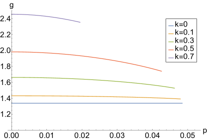
In Fig. 1 numerical values as a function of and doping are plotted. This is done by solving from the Luttinger constraint (24),(25) and then evaluating (69). We found that for fixed there are two solutions for . The larger solution is physical because in the limit. The values are restricted to be inside the stability region plotted in Fig. 2.
4.4.2 sector
At , there are two degenerate eigenvectors with eigenvalue . Below we show that these two eigenvectors correspond to adding bosonic and fermionic charges, and therefore their corrections in the IR can be absorbed into and .
We show that the charge modes span the eigenspace of . The charges are determined by and through the Luttinger constraints (24),(25). The charge modes are variations of the Green’s function, which is
| (70) |
where the variations of come from explicit dependence on and implicit dependence through the prefactor . Evaluating on the explicit form of Green’s function (22), we have
| (71) |
The ’s can be determined from ’s by differentiating (23)
| (72) |
4.5 Stability constraints of the conformal solution
In this subsection we use the resonance theory to analyze stability constraints of the conformal solution (22) and derive bounds on the and doping density in the large limit. We consider the following two criteria for stable.
-
1.
The conformal solution should be stable against UV perturbations, i.e. UV sources should be irrelevant. A resonant for which has eigenvalue one corresponds to an operator with scaling dimension in the conformal filed theory. Therefore, should have no resonance within , and follows from symmetry of .
- 2.
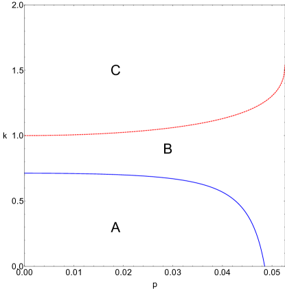
The outcome of the above constraints is the diagram Fig. 2 in space, where only region A is stable. Region B violates constraint 1 and region C violates constraint 2. Therefore if the conformal solution is stable against UV perturbations, it is automatically stable against the other conformal solution. This agrees with the renormalization group analysis in [24] that the fixed point is stable and the fixed point is a saddle point. Therefore the leading UV corrections to Green’s function in the stable region indeed come from the resonance.
Below we will elaborate on how these constraints are implemented. To find resonance, we analyze zeroes of the function
| (74) |
where the values of are determined by through the Luttinger constraints (24), (25). There are two solutions for and we choose the larger one which has the correct limiting behavior as . We have also chosen and such that the spectral constraint , is fulfilled. Due to the symmetry, we focus on the case. Typical behaviors of is shown in Fig. 3.


In region A the first two zeroes of is exactly at and and the conformal solution is stable. When we go from region A to region B, the pole at switches sign and a zero develops between . This zero corresponds some relevant operator in the UV source which destabilize the conformal solution. Therefore constraint 1 can be implemented as requiring the pole (4th order) of at should have negative coefficient, which is equivalent to
| (75) |
The above condition yields the curve separating region A and region B.
When we further increase and go to region C, the previous zero in is now shifted to ( is divergent). This resonance appearing between can be interpreted as the fermion operator in the phase. At the transition point switches sign. The condition is in fact algebraically equivalent to the condition that (23) has real solutions for . The latter requires
| (76) |
The LHS is actually a factor of and all the other factors are negative definite. Therefore (76) implements constraint 2 and gives the boundary between region B and region C.
5 Finite temperature generalization
The corrections obtained in the previous section are only valid for zero temperature, and in this section we will generalize them to finite temperature. Because the matrices and are not only SL(2,) covariant but also reparameterization and covariant, the eigenvector coefficients and the eigenvalues are the same at finite temperature. However, the power law in the ansatz (50) shall be replaced by its counterpart on the thermal circle, which we now calculate.
In the zero temperature resonance formalism, the eigenfunctions are written in a basis and branch. It is convenient at zero temperature as conformal transformations doesn’t mix positive and negative times. However this is not so at finite temperature because branches have to connect and they are not independent. We instead choose to restrict functions on the interval ( and in this part we take thermal circle size ), and consider symmetric and antisymmetric functions on this interval. Also, this approach applies to both bosons and fermions because they only differ by how the function should be continued beyond .
First, we need to generalize the Green’s function to finite temperature, this can be achieved by a combination of reparameterization and gauge transformation. The result is
| (77) |
where is determined by
| (78) |
where indicate the periodicity of , and .
The corrections are eigenfunctions of the kernel . It is argued in [34] using star-triangle transformations that these eigenfunctions can be derived from conformal three-point functions
| (79) |
where is an operator of scaling dimension , and denotes the fermions and bosons. The resonant response corresponds to and a discrete spectrum of . There are two kinds of three-point functions which yield symmetric/antisymmetric corrections under :
| (80) | |||||
| (81) |
Here we have neglected prefactors and the spectral asymmetry , because these factors are absorbed into in (79). The factor will also be absorbed into , and therefore the following terms contribute to :
| (82) | |||||
| (83) |
The symmetric function has been studied in [34], and we reproduce the analysis here. To evaluate the integral, we switch to complex variable , and analytical continue
After some manipulations, we obtain
| (84) |
where .
The integrand above has branch points at . We need to regulate the integral in a symmetrical manner with respect to . To do so, we choose to replace , which amounts to splitting each branch point into two, and then we can choose a symmetrical branch cut as shown in Fig. 4. After that, we deform the integration contour into two loops that winds around the two branch cuts. Along the branch cuts respectively, the integral (84) becomes the Euler integral representation of hypergeometric functions, and we obtain
| (85) |
| (86) |
Here the in means we analytically continue from through upper/lower half-plane. The calculation of is similar. The difference is that the integrand switches sign when we passes or , so the prefactors of hypergeometric functions change. The result is
| (87) |
| (88) |
To extract the asymptotics, we need to take the limit. This is more transparent after applying transformation formulae of hypergeometric functions to and :
| (89) | |||||
| (90) | |||||
where , analytically continued from through upper half plane. In the above two equations, the first terms can be interpreted as a UV response, and the second terms can be interpreted as IR response. Taking the limit for the IR term, we obtain the asymptotics
| (91) | |||||
| (92) |
The above results indicate that we can make the following replacement in the ansatz (50):
| (93) | |||||
| (94) |
The case of interest is , and we have
| (95) | |||||
| (96) |
Here .
As a sanity check, we also look at , which yields
| (97) | |||||
| (98) |
As discussed previously perturbation corresponds to adding charge to the system, which will introduce a factor in the Green’s function, and this matches the solution of
It is unspecified that how and should continue beyond , and we are free to choose periodic or antiperiodic boundary condition by including factors. Noticing that the original function is defined on , when we periodically continue it to , it transforms the function it multiplies between periodic and antiperiodic boundary conditions.
Taking periodicity into account, we propose that the Green’s function correction should have the following form
| (99) |
If we assume that the resonance theory described in previous section is reparameterization and covariant, the eigenvalues and eigenvectors should carry over to the current finite temperature setting. If this is true, we can determine the coefficients and from by a basis change . The result for correction is therefore
| (100) | |||||
| (101) |
For the particle-hole symmetric case relevant to the metal-insulator transition [25], we have , therefore
| (102) | |||||
| (103) |
6 Evaluation of the conductivity
In this section we compute the leading correction to resistivity due to resonance.
The electron Green’s function is
| (104) |
where and the prefactor is
| (105) |
Here are some useful integrals for evaluating the Fourier transforms of and :
| (107) | ||||
| (108) | ||||
| (109) | ||||
| (110) | ||||
| (111) | ||||
| (112) |
Here (107) and (110) are derived using contour integral along the unit circle of , and the cut is from to . The integration contour can be deformed to be , which becomes standard integral representation of beta function and generalized hypergeometric function. (108) and (109) are derived from (107) by integration by parts. (111) and (112) follows from (110) by definition. For correction we will be using Eqs.(107)-(109).
In presence spectral asymmetry we should put with in Eqs.(107)-(109). The electron Green’s function corresponds to , which has log-divergence at the UV. We regulate the divergence using expansion:
| (113) | |||||
| (114) |
| (115) |
where is the harmonic number, and is -th derivative of digamma function . The poles in translates to some log terms in which depends on UV behavior of .
Let us compute the spectral density of the above integrals , which yields
| (116) | |||||
| (117) | |||||
| (118) |
The electron spectral density is (we restored the temperature by replacing )
| (119) |
where is given in (105).
The correction due to mode is (we have inserted a factor to ensure correct dimensionality)
| (120) |
The conductivity is
| (121) |
The background term is
| (122) |
The correction term is
| (123) |
where the term in doesn’t contribute as its integrand is an odd function of . The resistivity is therefore
| (124) |
with slope and .
We know that the coefficient of the Schwarzian action is related to heat capacity by [32, 40]
| (125) |
so we have the relation which reduces to (4)
| (126) |
where the ratio is given in (69). From numerical values of shown in Fig. 1, (126) is positive for all consistent with stability constraints discussed in Sec. 4.5.
7 Conclusions
We have discussed a class of deconfined critical points of electronic models on large dimension lattices with random nearest exchange interactions with zero mean [24, 25]. These critical points are solvable in a large limit in which the spin symmetry is generalized from SU(2) to SU(). They can also be analyzed by renormalization group methods [24], but we did not use that approach here.
The key feature of these critical points is that the critical theory has an emergent time reparameterization symmetry. This symmetry is broken by ‘dangerously irrelevant’ terms in the action, in a condensed matter terminology [41, 42], to a SL(2,) symmetry of the low state. Such a softly broken reparameterization mode is described by an effective Schwarzian action. One important consequence of this soft mode is that correlators of primary operators have a correction in the form of (1), with related to the co-efficient of the Schwarzian term. These are all features that the models considered here share with the SYK models [22, 32, 33, 34, 35], and they are expected to apply more broadly to other critical theories with a time reparameterization symmetry. In particular, they are also expected to hold beyond the large limit employed by us.
Turning from (1) to the resistivity, we consider the generality of the structure in (2). We discuss some features in turn:
-
1.
The conformal theory yields a -independent ‘residual’ resistivity as . We noted that this was a consequence of decay of the electron Green’s function i.e. the scaling dimension for the electron operator [26, 24]. This feature is expected to hold at deconfined critical points beyond the large limit, and was also found in the all-loop renormalization group analysis of Joshi et al. [24].
-
2.
The leading correction to is linear in as . This follows directly from inserting (1) into the Kubo formula, and is also generally true, beyond the large limit. This makes the time reparameterization soft mode a promising and generic mechanism for the ubiquitous low linear-in- resistivity in correlated electron compounds.
-
3.
There is a universal relationship between the co-efficient of the linear resistivity and the product of and the co-efficient of the linear in temperature specific heat. Unlike the other features just noted, this is expected to only hold in the large limit. It relies on the momentum independence of in (28), which is not present in the large but general expression in (27). More generally, we do expect that the coefficient of the linear- resistivity will be proportional to , but the proportionality constant will be non-universal.
- 4.
-
5.
The linear power-law of resistivity with temperature is robustly pinned to a scaling dimension associated with the time reparameterization mode. This is in contrast to other mechanisms for non-Fermi liquid transport, where the resistivity has a power-law in temperature related to the scaling dimensions of various model-specific operators [14, 15, 16, 17, 18, 19, 43, 44, 45] which can take diverse values.
We conclude by mentioning other contexts in which time reparameterization plays a role:
-
1.
We recall that the time reparameterization soft mode also plays a key role in the holographic connections of SYK-like models to the quantum gravity theory of black holes with a near-horizon AdS2 geometry [46, 38]: it maps onto quantum fluctuations of the boundary between the near and far horizon regions [22, 47, 34, 48, 49, 50].
-
2.
The theory of Fermi surfaces in two spatial dimensions coupled to gapless bosons (order parameters or gauge fields) [51, 52, 53, 54, 55] has the important feature that the canonical time derivative terms scale to zero at criticality, like the time derivative terms in (13). Consequently, these critical theories also have an emergent time reparameterization symmetry [56], and it would be interesting to explore the consequences.
Acknowledgements
We thank D. Chowdhury, A. Georges, O. Parcollet, A. A. Patel, G. Tarnopolsky, and M. Tikhanovskaya for valuable discussions. This research was supported by the U.S. Department of Energy under Grant DE-SC0019030. Y.G. is supported by the Gordon and Betty Moore Foundation EPiQS Initiative through Grant GBMF-4306.
Appendix A Alternative large limit
This appendix contrasts our approach from the distinct large limit of the same model taken by Parcollet and Georges [13]. Their procedure does not introduce the orbital index, and (5) is replaced by
| (127) |
Consequently, the constraints in (8) and (9) are replaced by
| (128) |
In such a large limit, the boson is always condensed at any non-zero , and does not fluctuate. Consequently we can just replace the boson operator by a c-number . Another important difference, needed because of the boson condensation, is that the hopping scales differently with : instead of (12) they have
| (129) |
With condensed, the ground state of the large limit of Ref. [13] is always a Fermi liquid. They also examined the behavior at non-zero , and found that there is a crossover to a non-Fermi liquid above a coherence temperature . Moreover, they found a linear-in- resistivity for , but with a mechanism different from that in the present paper; note that their linear- resistivity does not extend down to at any coupling or density. Their momentum-dependent Green’s function replaces (27) by
| (130) |
Ref. [13] showed that , and so all three terms in (130) have the same scaling in . Specifically, there saddle point equations are
| (131) |
These equations should be compared with our saddle point equations (21) and (16)-(19): the non-Fermi liquid behavior arises entirely from , and there is no . Combining (130) and (131), we obtain their result
| (132) |
which shows that there is no net electron self-energy from the term, apart from a renormalization of the hopping from to ; this feature is quite different from our large limit. The absence of an electron self-energy from leads to a vanishing residual resistivity in the large limit of this appendix [13].
References
- Takagi et al. [1992] H. Takagi, B. Batlogg, H. L. Kao, J. Kwo, R. J. Cava, J. J. Krajewski, and W. F. Peck, “Systematic evolution of temperature-dependent resistivity in ,” Phys. Rev. Lett. 69, 2975 (1992).
- Taillefer [2010] L. Taillefer, “Scattering and Pairing in Cuprate Superconductors,” Annual Review of Condensed Matter Physics 1, 51 (2010), arXiv:1003.2972 [cond-mat.supr-con] .
- Bruin et al. [2013] J. A. N. Bruin, H. Sakai, R. S. Perry, and A. P. Mackenzie, “Similarity of Scattering Rates in Metals Showing -Linear Resistivity,” Science 339, 804 (2013).
- Sarkar et al. [2017] T. Sarkar, P. R. Mandal, J. S. Higgins, Y. Zhao, H. Yu, K. Jin, and R. L. Greene, “Fermi surface reconstruction and anomalous low-temperature resistivity in electron-doped La2-xCexCuO4,” Phys. Rev. B 96, 155449 (2017), arXiv:1706.07836 [cond-mat.supr-con] .
- Brown et al. [2019] P. T. Brown, D. Mitra, E. Guardado-Sanchez, R. Nourafkan, A. Reymbaut, C.-D. Hébert, S. Bergeron, A. M. S. Tremblay, J. Kokalj, D. A. Huse, P. Schauß, and W. S. Bakr, “Bad metallic transport in a cold atom Fermi-Hubbard system,” Science 363, 379 (2019), arXiv:1802.09456 [cond-mat.quant-gas] .
- Legros et al. [2018] A. Legros, S. Benhabib, W. Tabis, F. Laliberté, M. Dion, M. Lizaire, B. Vignolle, D. Vignolles, H. Raffy, Z. Z. Li, P. Auban-Senzier, N. Doiron-Leyraud, P. Fournier, D. Colson, L. Taillefer, and C. Proust, “Universal -linear resistivity and Planckian dissipation in overdoped cuprates,” Nature Physics 15, 142 (2018), arXiv:1805.02512 [cond-mat.supr-con] .
- Cao et al. [2020] Y. Cao, D. Chowdhury, D. Rodan-Legrain, O. Rubies-Bigorda, K. Watanabe, T. Taniguchi, T. Senthil, and P. Jarillo-Herrero, “Strange Metal in Magic-Angle Graphene with near Planckian Dissipation,” Phys. Rev. Lett. 124, 076801 (2020), arXiv:1901.03710 [cond-mat.str-el] .
- Nakajima et al. [2019] Y. Nakajima, T. Metz, C. Eckberg, K. Kirshenbaum, A. Hughes, R. Wang, L. Wang, S. R. Saha, I.-L. Liu, N. P. Butch, D. Campbell, Y. S. Eo, D. Graf, Z. Liu, S. V. Borisenko, P. Y. Zavalij, and J. Paglione, “Planckian dissipation and scale invariance in a quantum-critical disordered pnictide,” arXiv e-prints (2019), arXiv:1902.01034 [cond-mat.str-el] .
- Mukerjee et al. [2006] S. Mukerjee, V. Oganesyan, and D. Huse, “Statistical theory of transport by strongly interacting lattice fermions,” Phys. Rev. B 73, 035113 (2006), arXiv:cond-mat/0503177 [cond-mat.str-el] .
- Deng et al. [2013] X. Deng, J. Mravlje, R. Žitko, M. Ferrero, G. Kotliar, and A. Georges, “How Bad Metals Turn Good: Spectroscopic Signatures of Resilient Quasiparticles,” Phys. Rev. Lett. 110, 086401 (2013), arXiv:1210.1769 [cond-mat.str-el] .
- Werman et al. [2017a] Y. Werman, S. A. Kivelson, and E. Berg, “Non-quasiparticle transport and resistivity saturation: a view from the large- limit,” npj Quantum Materials 2, 7 (2017a), arXiv:1607.05725 [cond-mat.str-el] .
- Werman et al. [2017b] Y. Werman, S. A. Kivelson, and E. Berg, “Quantum chaos in an electron-phonon bad metal,” (2017b), arXiv:1705.07895 [cond-mat.str-el] .
- Parcollet and Georges [1999] O. Parcollet and A. Georges, “Non-Fermi-liquid regime of a doped Mott insulator,” Phys. Rev. B 59, 5341 (1999), arXiv:cond-mat/9806119 .
- Zhang [2017] P. Zhang, “Dispersive Sachdev-Ye-Kitaev model: Band structure and quantum chaos,” Phys. Rev. B 96, 205138 (2017), arXiv:1707.09589 [cond-mat.str-el] .
- Song et al. [2017] X.-Y. Song, C.-M. Jian, and L. Balents, “Strongly Correlated Metal Built from Sachdev-Ye-Kitaev Models,” Phys. Rev. Lett. 119, 216601 (2017), arXiv:1705.00117 [cond-mat.str-el] .
- Patel et al. [2018] A. A. Patel, J. McGreevy, D. P. Arovas, and S. Sachdev, “Magnetotransport in a model of a disordered strange metal,” Phys. Rev. X 8, 021049 (2018), arXiv:1712.05026 [cond-mat.str-el] .
- Chowdhury et al. [2018] D. Chowdhury, Y. Werman, E. Berg, and T. Senthil, “Translationally invariant non-Fermi liquid metals with critical Fermi-surfaces: Solvable models,” Phys. Rev. X 8, 031024 (2018), arXiv:1801.06178 [cond-mat.str-el] .
- Guo et al. [2019] H. Guo, Y. Gu, and S. Sachdev, “Transport and chaos in lattice Sachdev-Ye-Kitaev models,” Phys. Rev. B 100, 045140 (2019), arXiv:1904.02174 [cond-mat.str-el] .
- Patel and Sachdev [2019] A. A. Patel and S. Sachdev, “Theory of a Planckian metal,” Phys. Rev. Lett. 123, 066601 (2019), arXiv:1906.03265 [cond-mat.str-el] .
- Cha et al. [2019] P. Cha, A. A. Patel, E. Gull, and E.-A. Kim, “-linear resistivity in models with local self-energy,” arXiv e-prints , arXiv:1910.07530 (2019), arXiv:1910.07530 [cond-mat.str-el] .
- Sachdev and Ye [1993] S. Sachdev and J. Ye, “Gapless spin-fluid ground state in a random quantum Heisenberg magnet,” Phys. Rev. Lett. 70, 3339 (1993), arXiv:cond-mat/9212030 .
- Kitaev [2015] A. Y. Kitaev, “Talks at KITP, University of California, Santa Barbara,” Entanglement in Strongly-Correlated Quantum Matter (2015).
- Cha et al. [2020] P. Cha, N. Wentzell, O. Parcollet, A. Georges, and E.-A. Kim, “Linear resistivity and Sachdev-Ye-Kitaev (SYK) spin liquid behavior in a quantum critical metal with spin- fermions,” (2020), arXiv:2002.07181 [cond-mat.str-el] .
- Joshi et al. [2019] D. G. Joshi, C. Li, G. Tarnopolsky, A. Georges, and S. Sachdev, “Deconfined critical point in a doped random quantum Heisenberg magnet,” Phys. Rev. X to appear (2019), arXiv:1912.08822 [cond-mat.str-el] .
- Tarnopolsky et al. [2020] G. Tarnopolsky, C. Li, D. G. Joshi, and S. Sachdev, “Metal-insulator transition in a random Hubbard model,” (2020), arXiv:2002.12381 [cond-mat.str-el] .
- Fu et al. [2018] W. Fu, Y. Gu, S. Sachdev, and G. Tarnopolsky, “ fractionalized phases of a solvable, disordered, - model,” Phys. Rev. B 98, 075150 (2018), arXiv:1804.04130 [cond-mat.str-el] .
- Florens and Georges [2002] S. Florens and A. Georges, “Quantum impurity solvers using a slave rotor representation,” Physical Review B 66, 165111 (2002), arXiv:cond-mat/0206571 [cond-mat.str-el] .
- Haule et al. [2002] K. Haule, A. Rosch, J. Kroha, and P. Wölfle, “Pseudogaps in an Incoherent Metal,” Phys. Rev. Lett. 89, 236402 (2002), arXiv:cond-mat/0205347 [cond-mat.str-el] .
- Haule et al. [2003] K. Haule, A. Rosch, J. Kroha, and P. Wölfle, “Pseudogaps in the - model: An extended dynamical mean-field theory study,” Phys. Rev. B 68, 155119 (2003), arXiv:cond-mat/0304096 [cond-mat.str-el] .
- Florens and Georges [2004] S. Florens and A. Georges, “Slave-rotor mean-field theories of strongly correlated systems and the Mott transitionin finite dimensions,” Physical Review B 70, 035114 (2004), arXiv:cond-mat/0404334 [cond-mat.str-el] .
- Florens et al. [2013] S. Florens, P. Mohan, C. Janani, T. Gupta, and R. Narayanan, “Magnetic fluctuations near the Mott transition towards a spin liquid state,” EPL 103, 17002 (2013), arXiv:1006.3620 [cond-mat.str-el] .
- Maldacena and Stanford [2016] J. Maldacena and D. Stanford, “Remarks on the Sachdev-Ye-Kitaev model,” Phys. Rev. D 94, 106002 (2016), arXiv:1604.07818 [hep-th] .
- Bagrets et al. [2016] D. Bagrets, A. Altland, and A. Kamenev, “Sachdev–Ye–Kitaev model as Liouville quantum mechanics,” Nucl. Phys. B 911, 191 (2016), arXiv:1607.00694 [cond-mat.str-el] .
- Kitaev and Suh [2018] A. Kitaev and S. J. Suh, “The soft mode in the Sachdev-Ye-Kitaev model and its gravity dual,” JHEP 05, 183 (2018), arXiv:1711.08467 [hep-th] .
- Gu et al. [2020] Y. Gu, A. Kitaev, S. Sachdev, and G. Tarnopolsky, “Notes on the complex Sachdev-Ye-Kitaev model,” JHEP 02, 157 (2020), arXiv:1910.14099 [hep-th] .
- Georges et al. [2000] A. Georges, O. Parcollet, and S. Sachdev, “Mean Field Theory of a Quantum Heisenberg Spin Glass,” Phys. Rev. Lett. 85, 840 (2000), cond-mat/9909239 .
- Georges et al. [2001] A. Georges, O. Parcollet, and S. Sachdev, “Quantum fluctuations of a nearly critical Heisenberg spin glass,” Phys. Rev. B 63, 134406 (2001), cond-mat/0009388 .
- Sachdev [2015] S. Sachdev, “Bekenstein-Hawking Entropy and Strange Metals,” Phys. Rev. X 5, 041025 (2015), arXiv:1506.05111 [hep-th] .
- Georges et al. [1996] A. Georges, G. Kotliar, W. Krauth, and M. J. Rozenberg, “Dynamical mean-field theory of strongly correlated fermion systems and the limit of infinite dimensions,” Rev. Mod. Phys. 68, 13 (1996).
- Davison et al. [2017] R. A. Davison, W. Fu, A. Georges, Y. Gu, K. Jensen, and S. Sachdev, “Thermoelectric transport in disordered metals without quasiparticles: The Sachdev-Ye-Kitaev models and holography,” Phys. Rev. B 95, 155131 (2017), arXiv:1612.00849 [cond-mat.str-el] .
- Senthil et al. [2004] T. Senthil, A. Vishwanath, L. Balents, S. Sachdev, and M. P. A. Fisher, “Deconfined Quantum Critical Points,” Science 303, 1490 (2004), arXiv:cond-mat/0311326 [cond-mat.str-el] .
- Senthil et al. [2005] T. Senthil, L. Balents, S. Sachdev, A. Vishwanath, and M. P. A. Fisher, “Deconfined Criticality Critically Defined,” J. Phys. Soc. Jpn. 74, 1 (2005), arXiv:cond-mat/0404718 [cond-mat.str-el] .
- Faulkner et al. [2010] T. Faulkner, N. Iqbal, H. Liu, J. McGreevy, and D. Vegh, “Strange Metal Transport Realized by Gauge/Gravity Duality,” Science 329, 1043 (2010).
- Patel and Sachdev [2014] A. A. Patel and S. Sachdev, “DC resistivity at the onset of spin density wave order in two-dimensional metals,” Phys. Rev. B 90, 165146 (2014), arXiv:1408.6549 [cond-mat.str-el] .
- Hartnoll et al. [2014] S. A. Hartnoll, R. Mahajan, M. Punk, and S. Sachdev, “Transport near the Ising-nematic quantum critical point of metals in two dimensions,” Phys. Rev. B 89, 155130 (2014), arXiv:1401.7012 [cond-mat.str-el] .
- Sachdev [2010] S. Sachdev, “Holographic metals and the fractionalized Fermi liquid,” Phys. Rev. Lett. 105, 151602 (2010), arXiv:1006.3794 [hep-th] .
- Maldacena et al. [2016] J. Maldacena, D. Stanford, and Z. Yang, “Conformal symmetry and its breaking in two dimensional Nearly Anti-de-Sitter space,” PTEP 2016, 12C104 (2016), arXiv:1606.01857 [hep-th] .
- Moitra et al. [2019] U. Moitra, S. P. Trivedi, and V. Vishal, “Extremal and near-extremal black holes and near-CFT1,” JHEP 07, 055 (2019), arXiv:1808.08239 [hep-th] .
- Sachdev [2019] S. Sachdev, “Universal low temperature theory of charged black holes with AdS2 horizons,” J. Math. Phys. 60, 052303 (2019), arXiv:1902.04078 [hep-th] .
- Iliesiu and Turiaci [2020] L. V. Iliesiu and G. J. Turiaci, “The statistical mechanics of near-extremal black holes,” (2020), arXiv:2003.02860 [hep-th] .
- Lee [2018] S.-S. Lee, “Recent Developments in Non-Fermi Liquid Theory,” Annual Review of Condensed Matter Physics 9, 227 (2018), arXiv:1703.08172 [cond-mat.str-el] .
- Lee [2009] S.-S. Lee, “Low energy effective theory of Fermi surface coupled with U(1) gauge field in 2+1 dimensions,” Phys. Rev. B80, 165102 (2009), arXiv:0905.4532 [cond-mat.str-el] .
- Metlitski and Sachdev [2010] M. A. Metlitski and S. Sachdev, “Quantum phase transitions of metals in two spatial dimensions. I. Ising-nematic order,” Phys. Rev. B 82, 075127 (2010), arXiv:1001.1153 [cond-mat.str-el] .
- Mross et al. [2010] D. F. Mross, J. McGreevy, H. Liu, and T. Senthil, “A controlled expansion for certain non-Fermi liquid metals,” Phys. Rev. B 82, 045121 (2010), arXiv:1003.0894 [cond-mat.str-el] .
- Metlitski and Sachdev [2010] M. A. Metlitski and S. Sachdev, “Quantum phase transitions of metals in two spatial dimensions: II. Spin density wave order,” Phys. Rev. B 82, 075128 (2010), arXiv:1005.1288 [cond-mat.str-el] .
- [56] A. A. Patel and S. Sachdev, unpublished .