Radio-emission of axion stars

Abstract

We study parametric instability of compact axion dark matter structures decaying to radiophotons. Corresponding objects — Bose (axion) stars, their clusters, and clouds of diffuse axions — form abundantly in the postinflationary Peccei-Quinn scenario. We develop general description of parametric resonance incorporating finite-volume effects, backreaction, axion velocities and their (in)coherence. With additional coarse-graining, our formalism reproduces kinetic equation for virialized axions interacting with photons. We derive conditions for the parametric instability in each of the above objects, as well as in collapsing axion stars, evaluate photon resonance modes and their growth exponents. As a by-product, we calculate stimulated emission of Bose stars and diffuse axions, arguing that the former can give larger contribution into the radiobackground. In the case of QCD axions, the Bose stars glow and collapsing stars radioburst if the axion-photon coupling exceeds the original KSVZ value by two orders of magnitude. The latter constraint is alleviated for several nearby axion stars in resonance and absent for axion-like particles. Our results show that the parametric effect may reveal itself in observations, from FRB to excess radiobackground.

I Introduction

The QCD axion Kim:2008hd and similar particles pdg are perfect dark matter candidates Sikivie:2006ni ; Arias:2012az : they are motivated Peccei:1977hh ; Arvanitaki:2009fg and have tiny interactions diCortona:2015ldu , including coupling to the electromagnetic field. But the same interactions — alas — make the axions “invisible” dictating overly precise detection measurements Irastorza:2018dyq ; Armengaud:2019uso and limiting possible observational effects Arvanitaki:2014wva ; Arza:2019nta ; Foster:2020pgt .

Nevertheless, under certain conditions an avalanche of exponentially growing photon number ${n_{\gamma}\propto\exp\{2\mu_{\infty}t\}}$ can appear in the axionic medium Tkachev:1987cd , with growth exponent $\mu_{\infty}$ proportional to the axion-photon coupling and axion field strength. This process is known as parametric resonance. It occurs because the axions decay into photons which stimulate decays of more axions. In the infinite volume parametric axion-photon conversion is well understood, but does not occur during cosmological evolution of the axion field Preskill:1982cy ; Abbott:1982af ; Alonso-Alvarez:2019ssa . In compact volume of size $L$ the avalanche appears if the photon stimulates at least one axion decay as it passes the object length Tkachev:1987cd ; Riotto:2000kh . This gives order-of-magnitude resonance condition,

$$\mu_{\infty}L\gtrsim 1\;.$$ (1)

Unfortunately, apart from this intuitive estimate and brute-force numerical computations Kephart:1994uy ; Tkachev:2014dpa ; Hertzberg:2018zte ; Arza:2018dcy ; Sigl:2019pmj ; Carenza:2019vzg ; Chen:2020ufn ; Wang:2020zur ; Arza:2020eik , no consistent quantitative theory of axion-photon conversion in finite-size objects has been developed so far.

In this paper we fill this gap with a general, detailed, and usable quasi-stationary approach to parametric resonance in a finite volume. Our method works only for nonrelativistic axions, but accounts for their coherence, or its absence, axion velocities, binding energy and gravitational redshift, backreaction of photons on axions, and arbitrary volume shape. In the limit of diffuse axions it reproduces well-known axion-photon kinetic equation, if additional coarse-graining is introduced.

Notably, the cosmology of QCD axion Preskill:1982cy ; Abbott:1982af ; Dine:1982ah provides rich dark matter structure at small scales Niemeyer:2019aqm , with a host of potentially observable astrophysical implications. Namely, in the postinflationary scenario violent inhomogeneous evolution of the axion field during the QCD epoch Kolb:1993hw ; Klaer:2017ond ; Gorghetto:2018myk ; Vaquero:2018tib ; Buschmann:2019icd leads to formation of axion miniclusters Hogan:1988mp ; Kolb:1993zz ; Kolb:1994fi  — dense objects of typical mass $10^{-13}\,M_{\odot}$ forming hierarchically bound structures Eggemeier:2019khm . In the centers of miniclusters even denser compact objects, the axion (Bose) stars Ruffini:1969qy ; Tkachev:1986tr , appear due to gravitational kinetic relaxation Levkov:2018kau ; Eggemeier:2019jsu . Simulations suggest Levkov:2018kau ; Vaquero:2018tib ; Buschmann:2019icd ; Niemeyer:2019aqm ; Eggemeier:2019jsu that these objects are abundant in the Universe, though their present-day mass is still under study Eggemeier:2019jsu . Another example of dense object formed by the QCD axions is a cloud around the superradiant black hole Arvanitaki:2010sy ; Arvanitaki:2009fg ; Stott:2018opm , see also Rosa:2017ury .

Beyond the QCD axion, miniclusters Arias:2012az and Bose stars Schive:2014dra ; Schive:2014hza ; Amin:2019ums can be formed by the axion-like particles at very different length and mass scales.

In this paper we derive precise conditions for parametric resonance in the isolated axion stars, collapsing stars, their clusters, and in the clouds of diffuse axions. We find unstable electromagnetic modes and their growth exponents $\mu$. Contrary to what naive infinite-volume intuition might suggest, resonance in nonrelativistic compact objects develops with $\mu\ll\mu_{\infty}$. As a result, in many cases it glows in the stationary regime, burning an infinitesimally small fraction of extra axions at every moment, to keep the resonance condition marginally broken.

Our calculations suggest three interesting scenaria with different observational outcomes. In the first chain of events the axion-photon coupling is high and the threshold for parametric resonance is reached during growth of axion stars via Bose-Einstein condensation. Then all condensing axions will be converted into radio-emission with frequency equal to the axion half-mass. This paves the way for indirect axion searches.

Second, at somewhat smaller axion-photon coupling, attractive self-interactions of axions inside the growing stars may become important before the resonance threshold is reached. As a result, the stars collapse Chavanis:2011zi ; Zakharov12 ; Levkov:2016rkk , shrink and ignite the instability to photons on the way. Alternatively, several smaller axion stars may come close, suddenly meeting the resonance condition Hertzberg:2018zte . In these cases a short and powerful burst of radio-emission appears.

Amusingly, powerful and unexplained Fast Radio Bursts (FRB) are presently observed in the sky Petroff:2019tty . It is tempting to relate them to parametric resonance in collapsing axion stars Tkachev:2014dpa and see if the main characteristics can be met.

In the third, most conservative scenario all Bose stars are far away from the parametric resonance. Nevertheless, the effect of stimulated emission turns them into powerful radioamplifyers of ambient radiowaves at the axion half-mass frequency. We compute amplification coefficients for the Bose stars and diffuse axions and find that realistically, stimulated emission of the stars may give larger contribution into the radiobackground.

In Sec. II we introduce nonrelativistic approximation for axions and review essential properties of Bose stars. General description of parametric resonance in finite volume is developed in Sec. III. In Sec. IV it is applied to radio-emission of static axion stars, their pairs, and amplification of ambient radiation. In Secs. V and VI we study resonance in diffuse axions and consider the effect of moving axions / axion stars, in particular, resonance in collapsing stars. Concluding remarks are given in Sec. VII.

II Axion stars

The diversity of compact objects in axion cosmology offers many astrophysical settings where the parametric resonance may be expected. One can consider static Bose stars, collapsing, moving, or tidally disrupted stars, even axion miniclusters. To describe all this spectrum in one go, we implement two important approximations.

First we describe axions by the classical field $a(t,\,{\bf x})$ satisfying

$$\Box a+{\cal V}^{\prime}(a)=0\;.$$ (2)

This is valid at large occupation numbers. Interaction with the gravitational field in Eq. (2) is hidden in the covariant derivatives, and the scalar potential

$${\cal V}=\frac{m^{2}}{2}\,a^{2}-\frac{g_{4}^{2}m^{2}}{4!\,f_{a}^{2}}\,a^{4}+\dots$$ (3)

includes mass $m$ and quartic coupling $(g_{4}m/f_{a})^{2}$. Self-interaction of the QCD axion is attractive: ${f_{a}\simeq(75.5~{}\rm MeV)^{2}}/m$ and $g_{4}\simeq 0.59$ diCortona:2015ldu . Axion-like particles may have ${g_{4}\simeq 0}$.

Second, we work in nonrelativistic approximation,

$$a=\frac{f_{a}}{\sqrt{2}}\,\left[\psi(t,\,{\bf x})\,\mathrm{e}^{-imt}+\mathrm{h.c.}\right]\;,$$ (4)

where $\psi$ slowly depends on space and time. Namely, if $\lambda$ is the typical wavelength of axions,

$$\partial_{t}\psi\sim\psi/m\lambda^{2}\;,\qquad\partial_{\bf x}\psi\sim\psi/\lambda\;,\qquad\lambda m\gg 1\;.$$ (5)

In this approximation Eq. (2) reduces to nonlinear Schrödinger equation,

$$i\partial_{t}\psi=-\frac{\Delta}{2m}\,\psi+m\left(\Phi-\frac{g_{4}^{2}}{8}|\psi|^{2}\right)\psi\;,$$ (6)

where $\Phi$ is a nonrelativistic gravitational potential solving the Poisson equation

$$\Delta\Phi=4\pi\rho/M_{pl}^{2}\;,$$ (7)

and $\rho=m^{2}f_{a}^{2}|\psi|^{2}$ is the mass density of axions.

Note that the method of this paper is applicable only if both of the above conditions are satisfied: the axions are nonrelativistic and they have large occupation numbers. Dark matter axions meet these requirements, except under extreme conditions.

A central object of our study is a Bose (axion) star, a stationary solution to the Schrödinger-Poisson system

$$\psi=\mathrm{e}^{-i\omega_{s}t}\psi_{s}(r)\;,\qquad\qquad\Phi=\Phi_{s}(r),$$ (8)

where $\omega_{s}<0$ is the binding energy of axions and $r$ is the radial coordinate. Physically, Eq. (8) describes Bose-Einstein condensate of axions occupying a ground state in the collective potential well $\Phi_{s}(r)$. This object is coherent: the complex phase of $\psi_{s}$ does not depend on space and time. Below we consider parametric resonance in stationary and colliding stars.

Notably, the axion stars with the critical mass

$$M_{cr}\simeq 10.2\;\frac{f_{a}M_{pl}}{mg_{4}}$$ (9)

and heavier stars are unstable Chavanis:2011zi . In this case attractive self-interaction in Eq. (6) overcomes the quantum pressure and the star starts to shrink developing huge axion densities in the center Levkov:2016rkk . We will see that this may trigger explosive parametric instability.

III General formalism

III.1 Linear theory

In this Section we construct general quasi-stationary theory for narrow parametric resonance of radiophotons in the finite volume filled with axions. This technique was first developed and presented in Patras2018 ; Patras2019 . In contrast to the resonance in the infinite volume Preskill:1982cy ; Abbott:1982af ; Tkachev:1986tr which universally leads to the Mathieu equation, the finite-volume one is described by the eigenvalue problem with a rich variety of solutions.

Consider Maxwell’s equations for the electromagnetic potential $A_{\mu}$ in the axion background $a(t,{\bf x})$,

$$\partial_{\mu}\left(F_{\mu\nu}+g_{a\gamma\gamma}a\tilde{F}_{\mu\nu}\right)=0\;,$$ (10)

where $F_{\mu\nu}=\partial_{\mu}A_{\nu}-\partial_{\nu}A_{\mu}$, ${{\tilde{F}}_{\mu\nu}\equiv\epsilon_{\mu\nu\lambda\rho}F_{\lambda\rho}/2}$, and $g_{a\gamma\gamma}$ is the standard axion-photon coupling. Below we also use dimensionless coupling $g^{\prime}\equiv f_{a}g_{a\gamma\gamma}/2^{3/2}$.

In the infinite volume one describes the resonance in the plain-wave basis for the electromagnetic field Preskill:1982cy ; Abbott:1982af ; Tkachev:1986tr , while the axion star suggests spherical decomposition Hertzberg:2018zte . We want to develop general formalism, and simpler at the same time, usable in a large variety of astrophysical settings.

We therefore introduce two simplifications. First, the photons travel straight, with light-bending effects being subdominant in the axion background, cf. Blas:2019qqp ; McDonald:2019wou . Thus, the parametric resonance develops almost independently along different directions. Second, we consider non-relativistic axions decaying into photons of frequency $\omega_{\gamma}\approx m/2$ with a very narrow spread.

This suggests decomposition in the gauge $A_{0}=0$,

$$A_{i}=\int d\boldsymbol{n}\;C_{i}^{(\boldsymbol{n})}(t,{\bf x})\,\mathrm{e}^{im(\boldsymbol{n}{\bf x}+t)/2}+\mathrm{h.c.}\;,$$ (11)

where $i=\{x,\,y,\,z\}$ and the integral runs over all unit vectors $\mathbf{n}$. The amplitudes $C_{i}^{(\boldsymbol{n})}$ include photon frequency spread. Hence, they weakly depend on space and time,

$$\partial_{t,{\bf x}}|C_{i}^{(\boldsymbol{n})}|\sim\lambda^{-1}|C_{i}^{(\boldsymbol{n})}|\;,\qquad\lambda m\gg 1\;,$$ (12)

where $\lambda^{-1}$ is the typical momentum of axions in Eq. (5).

Using Eq. (11), one finds that in the eikonal limit (12) the field equation (10) couples only the waves moving in the opposite, i.e. $+\boldsymbol{n}$ and $-\boldsymbol{n}$, directions. As a result, identical and independent equations are produced for every pair of directions. This is manifestation of the simple fact that the axions decay into two back-to-back photons.

Indeed, leaving one arbitrary direction $z=(\boldsymbol{n}{\bf x})$ and its counterpart $-z$, we obtain the ansatz that passes the field equation Patras2018 ; Patras2019 ,

$$A_{i}=C_{i}^{+}\,\mathrm{e}^{im(z+t)/2}+C_{i}^{-}\,\mathrm{e}^{im(z-t)/2}+\mathrm{h.c.}\;,$$ (13)

where the shorthand notations ${C_{i}^{+}(t,\,{\bf x})=C_{i}^{(\boldsymbol{n})}}$ and $C_{i}^{-}(t,\,{\bf x})=[C_{i}^{(-\boldsymbol{n})}]^{*}$ are introduced. Namely, substituting Eq. (13) into Eq. (10) and using approximations (12), (5), we arrive to the closed system,

$$\partial_{t}C^{+}_{x}=\partial_{z}C^{+}_{x}+{ig^{\prime}}\,m\psi^{*}C^{-}_{y}\;,$$ (14a)

$$\partial_{t}C^{-}_{y}=-\partial_{z}C^{-}_{y}-{ig^{\prime}}\,m\psi C^{+}_{x}\;.$$ (14b)

The other two physical polarizations satisfy the same equations with $C^{+}_{x}\to C^{+}_{y}$ and $C^{-}_{y}\to-C^{-}_{x}$, while the longitudinal part is fixed by the Gauss law ${C_{z}^{\pm}=2i\partial_{\alpha}C_{\alpha}^{\pm}/m}$; here and below $\alpha=\{x,\,y\}$. Overall, we have four amplitudes $C_{\alpha}^{\pm}$ representing two photon polarizations propagating in the $+z$ and $-z$ directions.

Equations (14) should be solved for every orientation of $z$ axis, in search for the growing instability modes. After that the modes can be superimposed in Eq. (11) or, practically, only the one with the largest exponent can be kept.

In spherically symmetric Bose star all directions are equivalent and description simplifies — we have to study only one direction. Notably, in this case one can derive Eqs. (14) using spherical decomposition, see Appendix A.

There is a residual hierarchy in Eqs. (14) related to small axion velocities $v\sim(m\lambda)^{-1}\ll 1$. Indeed, the nonrelativistic background evolves slowly, ${\partial_{t}\psi\sim\psi/m\lambda^{2}}$, while the electromagnetic field changes fast, ${\partial_{t}C\sim C/\lambda}$. Thus, equations for $C$ can be solved with adiabatic ansatz,

$$C_{i}^{\pm}=\mathrm{e}^{\int\limits^{t}\mu(t^{\prime})\,dt^{\prime}}\,c_{i}^{\pm}(t,\,{\bf x})\;,$$ (15)

where the complex exponent $\mu$ and quasi-stationary amplitudes $c_{i}^{\pm}$ evolve on the same timescales $m\lambda^{2}$ as $\psi$. Corrections to the adiabatic evolution (15) become exponentially small as $v\to 0$.

Using representation (15) in Eqs. (14) and ignoring time derivatives of $\mu$ and $c_{i}^{\pm}$, we finally obtain the eigenvalue problem Patras2018 ; Patras2019 ,

$$\mu c^{+}_{x}=\partial_{z}c^{+}_{x}+{ig^{\prime}}\,m\psi^{*}\,c^{-}_{y}\;,$$ (16a)

$$\mu c^{-}_{y}=-\partial_{z}c^{-}_{y}-{ig^{\prime}}\,m\psi\,c^{+}_{x}\;,$$ (16b)

where equations for the two remaining amplitudes are again obtained by $c^{+}_{x}\to c^{+}_{y}$ and ${c^{-}_{y}\to-c^{-}_{x}}$.

If the axions live in a finite region and no electromagnetic waves come from infinity, one imposes boundary conditions

$$\left.c^{+}_{\alpha}\right|_{z\to+\infty}=\left.c^{-}_{\alpha}\right|_{z\to-\infty}=0\;,$$ (17)

see Eq. (13).

The spectral problem (16) determines the electromagnetic modes $\{c^{+}_{x},\,c^{-}_{y}\}$ and their growth exponents $\mu$. The latter are not purely imaginary at $\psi\neq 0$ because $2\times 2$ operator in the right-hand side of Eqs. (16), is not anti-Hermitean. That is why in certain cases resonance instabilities — modes with $\mathrm{Re}\,\mu>0$ satisfying the boundary conditions (17) — appear.

It is worth discussing two parametrically small corrections to Eqs. (14), (16). First, derivatives with respect to $x$ and $y$ are absent in these systems: they appear only in the next, $(m\lambda)^{-1}$ order, determining the section of the resonance ray in the $(x,\,y)$ plane. If needed, they can be recovered with the substitution

$$\partial_{z}\to\partial_{z}-\frac{i}{m}(\partial_{x}^{2}+\partial_{y}^{2})\;,$$ (18)

to solve the spectral problem in three dimensions.

If the axion distribution is not spherically-symmetric, one expects that the resonance ray is narrow in the $(x,\,y)$ plane. Indeed, according to the leading-order equations (14) electromagnetic field grows with different exponents $\mu$ at different $x$ and $y$. This means that wide wave packets shrink around the resonance line until the quantum pressure (18) becomes relevant.

Second, direct interaction of photons with nonrelativistic gravitational field can be included in Eqs. (14) by changing

$$\partial_{z}C_{\alpha}^{\pm}\to\left(\partial_{z}+im\,\Phi\right)C_{\alpha}^{\pm}\;.$$ (19)

However, one immediately rotates this contribution away, ${C_{\alpha}^{\pm}\to\exp\{-im\int^{z}dz^{\prime}\,\Phi(z^{\prime})\}\,C_{\alpha}^{\pm}}$, with remaining corrections suppressed by $(m\lambda)^{-2}$.

As an illustration, consider static homogeneous axion field $\psi$ in the infinite volume. Quasi-stationary equations (16), in this case give $\partial_{z}c_{\alpha}^{\pm}=0$ and time-independent $\mu=\mu_{\infty}$ of the form

$$\mu_{\infty}=g^{\prime}m\,|\psi|>0\;.$$ (20)

Thus, electromagnetic amplitudes in Eq. (15) grow exponentially with time indicating parametric resonance. Expression (20) reproduces well-known infinite-volume growth rate Preskill:1982cy ; Abbott:1982af ; Tkachev:1986tr ; Tkachev:1987cd ; Kephart:1994uy ; Riotto:2000kh ; Hertzberg:2018zte ; Sigl:2019pmj of the axion-photon resonance.

III.2 Nonlinear stage

Backreaction of photons on axions can be easily incorporated in the Schrödinger-Poisson system (5). To this end one substitutes the nonrelativistic ansatz (4), (13) into the equation for the axion field,

$$\Box a+{\cal V}^{\prime}(a)=-\frac{g_{a\gamma\gamma}}{4}\,F_{\mu\nu}\tilde{F}_{\mu\nu}\;,$$ (21)

and omits higher derivatives of $\psi$ and $C$. This gives,

$$i\partial_{t}\psi=-\frac{\Delta\psi}{2m}+m\Phi\psi-\frac{mg_{4}^{2}}{8}\,|\psi|^{2}\psi\\ -\frac{mg^{\prime}}{f_{a}^{2}}\,\epsilon_{\alpha\beta}\,C_{\alpha}^{-}C_{\beta}^{+*},$$ (22)

where the backreaction is represented by the new term in the right-hand side.

Let us show that the last term in the above equation changes the mass $M=m^{2}f_{a}^{2}\int d^{3}\boldsymbol{x}\,|\psi|^{2}$ of the axion cloud. Indeed, taking the time derivative of $M$ and using Eq. (22), we obtain energy conservation law,

$$\partial_{t}M=J_{in}-\int dxdy\,F_{a\to\gamma\gamma}\;,$$ (23)

where $J_{in}=-mf_{a}^{2}\int d^{2}\sigma^{i}\,\mathrm{Im}(\psi^{*}\partial_{i}\psi)$ is the mass of axions entering the system per unit time and

$$F_{a\to\gamma\gamma}=2{m^{3}g^{\prime}}\int dz\,\epsilon_{\alpha\beta}\,\mathrm{Im}(\psi^{*}C_{\alpha}^{-}C_{\beta}^{+*})$$ (24)

is the flux of produced photons. Below we will also use the electromagnetic Poynting fluxes at infinity,

$$F_{\gamma}^{\pm}=\mp m^{2}(|C_{x}^{\pm}|^{2}+|C_{y}^{\pm}|^{2})/2\;.$$ (25)

In conjunction with Eqs. (14) this gives conservation law for the electromagnetic energy, ${\partial_{t}E_{\gamma}=\int dxdy\,\left(F_{a\to\gamma\gamma}-[F_{\gamma}^{+}+F_{\gamma}^{-}]_{z=-\infty}^{z=+\infty}\right)}$.

To conclude, one can numerically solve Eq. (22) together with Eqs. (14) and watch the axions burn abundantly.

IV Static coherent axions

IV.1 Condition for resonance

For a start, consider the case when the axions in a finite volume are coherent and do not move. A notable example of this situation is a static axion star.

Parametric resonance in this setup is presently understood at the qualitative level Tkachev:1987cd ; Tkachev:2014dpa ; Hertzberg:2018zte . Indeed, photons passing through the axions stimulate their decays ${a\to 2\gamma}$. The photon flux grows exponentially, ${F_{\gamma}\propto\exp\{2\mu_{\infty}t\}}$, and the secondary flux of backward-moving photons appears. After the original photons escape the region with axions, stimulated decays continue in the secondary flux moving in the opposite direction, etc, see Fig. 1. Overall, the back-and-forth motion inside the axion cloud accumulates photons at every pass if Eq. (1) is valid, i.e.

$$\mu_{\infty}L=g^{\prime}m|\psi|L\,\gtrsim 1\;,$$ (26)

where $L$ is the typical size of the cloud.

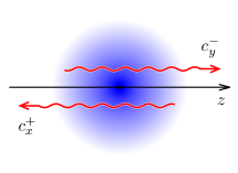
Figure 1: Parametric resonance in the axion star.

Our equations (14) reflect the same physics. Namely, consider the localized wave packet $C^{-}_{y}(t,\,{\bf x})$ going through axions in the $+z$ direction. Due to Eq. (14a) it creates the packet $C^{+}_{x}$ with the opposite group velocity which, in turn, produces $C^{-}_{y}$, etc. The photon flux grows exponentially during this process if unstable modes with $\mathrm{Re}\,\mu\geq 0$ are present.

Axion velocities are related to the complex phase of the field,

$$v_{i}=m^{-1}\partial_{i}\,\mathrm{arg}\,\psi\;.$$ (27)

In this section we assume that $\psi$ is real up to a constant phase which can be absorbed into redefinition of $c_{x}^{\pm}$ in Eqs. (16). This means that the axions are static and coherent.

In particular, the phase factor $\exp\{-i\omega_{s}t\}$ of the Bose star field (8) disappears from the electromagnetic equations after replacing $C_{i}^{\pm}\to C_{i}^{\pm}\mathrm{e}^{\pm i\omega_{s}t/2}$. Then the total binding energy $\omega_{s}$ of axions inside the star does not destroy the resonance, but slightly shifts its central frequency to

$$\omega_{\gamma}=(m+\omega_{s})/2\;,$$ (28)

see Eq. (13). Note that misconceptions regarding resonance blocking by gravitational and self-interaction energies still exist in the literature, e.g. Wang:2020zur .

At real $\psi$ the semiclassical eigenvalue problem (16) has two types of solutions. First, delocalized modes penetrate into the asymptotic regions $z\to\pm\infty$, where $\psi=0$ and $c_{i}^{\pm}\propto\exp(\pm\mu z)$. The exponents $\mu$ of these modes are purely imaginary, or their profiles would be unbounded. Physically, the delocalized modes represent electromagnetic waves coming from infinity. Second, there may exist localized modes satisfying the boundary conditions (17). They behave well at infinity if $\mathrm{Re}\,\mu\geq 0$. In addition, we prove in Appendix B that at real $\psi$ the exponents $\mu$ of these modes are real. The localized modes represent resonance instabilities.

In practical problems the resonance is not present in matter from the very beginning but appears in the course of nonrelativistic evolution. For example, the Bose stars form in slow galactic Schive:2014dra ; Schive:2014hza ; Veltmaat:2016rxo ; Veltmaat:2018dfz or minicluster Kolb:1993zz ; Eggemeier:2019jsu collapses, or afterwards in kinetic relaxation Levkov:2018kau , then grow kinetically at turtle-slow rates Levkov:2018kau ; Eggemeier:2019jsu ; Veltmaat:2019hou . Their subsequent evolution is also essentially nonrelativistic Schwabe:2016rze ; Schive:2019rrw .

At some point of quasi-stationary evolution one of purely imaginary eigenvalues $\mu$ may become real, and the parametric resonance develops. Let us discuss the borderline situation when the very first localized mode has $\mu=0$. The solution in this case is Patras2018 ; Patras2019 ,

$$c_{x}^{+}=A\cos D(z)\;,\quad c_{y}^{-}=-iA\sin D(z)\;,$$ (29)

where $A$ is a constant amplitude and

$$D(z)={g^{\prime}m}\int\limits_{-\infty}^{z}dz^{\prime}\,\psi(z^{\prime})\;.$$ (30)

Integration in Eq. (30) runs along the arbitrary-oriented $z$-axis.

The solution (29) satisfies the boundary conditions (17) if $D_{\infty}\equiv D(+\infty)=\pi/2$. At larger values of this integral the instability mode with positive $\mu$ exists. Thus, a precise condition for the parametric resonance along a given $z$-axis is

$$D_{\infty}\equiv{g^{\prime}m}\int\limits_{-\infty}^{+\infty}\psi(z)\,dz\geq\frac{\pi}{2}\;.$$ (31)

This concretizes the order-of-magnitude estimate (26). Recall that in our notations $\psi=\rho^{1/2}/(mf_{a})$, where $\rho$ is the mass density of axions.

Let us find out when the parametric resonance occurs in axion stars. In Appendix C we compute $D_{\infty}$ along the line passing through the star center, see Fig. 1. We consider two cases. First, if self-interactions of axions inside the star are negligible, Eq. (31) reads,

$$M_{s}\geq M_{s,\,0}=7.66\,\frac{M_{pl}}{mg_{a\gamma\gamma}}\;,\qquad\qquad g_{4}\approx 0\;,$$ (32)

where we restored $g_{a\gamma\gamma}=2^{3/2}g^{\prime}/f_{a}$. This condition is applicable in the axion-like models with $g_{4}=0$ or at $M_{s}\ll M_{cr}$. In these cases heavier stars are better for the resonance.

Second, if attractive self-interactions are present, the mass of the axion star is bounded from above, $M_{s}<M_{cr}$. Using the profile of the critical star in Eq. (31), we obtain condition

$$g_{a\gamma\gamma}>g_{a\gamma\gamma,\,0}\equiv 0.52\;\frac{g_{4}}{f_{a}}\;,\qquad M_{s}=M_{cr}\;,$$ (33)

cf. Hertzberg:2018zte ; Patras2018 . If this inequality is broken, parametric resonance does not develop in stable axion stars at all.

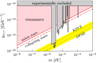
Figure 2: Masses and couplings of QCD axions needed for the Bose stars to develop parametric resonance (triangular shaded region above the solid line). The respective region for collapsing stars is above the dashed line.

For the parameters of QCD axion listed in Sec. II, the inequality (33) gives the shaded region in Fig. 2 marked “resonance.” Notably, the benchmark values diCortona:2015ldu of axion-photon coupling (KSVZ-DFSZ band in Fig. 2) are short by two orders of magnitude from igniting the resonance even in the critical star Tkachev:2014dpa ; Patras2018 ; Patras2018 Wang:2020zur . On the other hand, $g_{a\gamma\gamma}$ is model dependent, with the only constraint $g_{a\gamma\gamma}<f_{a}^{-1}$ coming from strong coupling in simple models Hook:2018dlk ; DiLuzio:2020wdo . Thus, even these simple models can satisfy (33) within the trustworthy parameter range. More elaborated (clockwork-inspired) QCD axion models Agrawal:2017cmd do not have these limitations and easily meet (33).

Alternatively, the self-coupling of the axion-like particles can be arbitrarily small. Condition (32) is then satisfied just for a sufficiently heavy star.

IV.2 Linear exponential growth

Let us find out how the resonance progresses. One does not expect it to turn immediately into an exponential catastrophe with $\mu\sim O(L^{-1})$, like the infinite-volume intuition might suggest, cf. Eq. (26). Rather, the electromagnetic field starts growing with parametrically small exponent $\mu\ll L^{-1}$ immediately after the condition (31) is met by the nonrelativistic evolution of axions. Initial values for this growth are tiny. They can be provided by the ambient radiation in astrophysical setup or, universally, by quantum fluctuations considered in Appendix D. In any case this initial stage proceeds linearly with no backreaction on axions.

We compute the growth exponent by solving the eigenvalue problem (16) perturbatively at small $\mu$, like in quantum mechanics. To this end we assume that the background $\psi(t,\,{\bf x})$ did not evolve much from the point $\psi_{0}({\bf x})\equiv\psi(t_{0},\,{\bf x})$ when the condition (31) was met, and the resonance mode is close to the solution (29). Calculation in Appendix B gives,

$$\mu=\frac{D_{\infty}-\pi/2}{\int dz\,\sin[2D_{0}(z)]}\;,$$ (34)

Here $D_{0}(z)$ is evaluated using $\psi_{0}({\bf x})$, a configuration at the rim of parametric instability, while $D_{\infty}$ uses $\psi$ in Eq. (31). Note that application of Eq. (34) essentially depends on nonrelativistic mechanism leading to resonance and providing $D_{\infty}-\pi/2=O(\psi-\psi_{0})$.

Expression (34) confirms that $\mu$ is indeed parametrically small and yet, large enough for the adiabatic regime (15) to take place. Generically, ${\psi-\psi_{0}\sim(t_{1}-t_{0})\,\partial_{t}\psi}$, where $t_{1}-t_{0}\sim\Lambda/\mu$ is the time from ignition of the resonance to the moment $t_{1}$ when the backreaction starts; ${\Lambda\sim\log[C^{\pm}(t_{1})/C^{\pm}(t_{0})]\sim 10^{2}}$ is a large logarithm. Then the nonrelativistic scaling (12), (5) and Eq. (34) give ${\mu\sim\lambda^{-1}(\Lambda/m\lambda)^{1/2}}$, where we also recalled that the resonance condition (31) is marginally satisfied. Thus,

$$(m\lambda^{2})^{-1}\ll\mu\ll\lambda^{-1}\;,$$

i.e. the electromagnetic fields evolve faster than the axion background but slower than the light-crossing time ${L^{-1}\sim\lambda^{-1}}$.

Applying Eq. (34) to the stationary axion star with $g_{4}\approx 0$, we get

$$\mu=0.197\;\frac{m^{2}}{M_{pl}^{2}}\,(M_{s}-M_{s,\,0})\;,$$ (35)

where Appendix C was consulted and $M_{s,\,0}$ is given in Eq. (32). Using this expression, one obtains $\mu\sim 10^{2}\;\mbox{s}^{-1}$ for $m=26\,\mu\mbox{eV}$ Klaer:2017ond and $\delta M_{s}\sim 10^{-13}\,M_{\odot}$. Thus, duration of the linear stage in QCD axion stars is one second or longer.

Figure 3: Luminosity $L_{\gamma}(t)=r^{2}\int d\Omega\,\boldsymbol{n}_{r}\,[\boldsymbol{E}\times\boldsymbol{H}]$ of axion star with $M_{s}\approx 1.04\,M_{s,\,0}$ during parametric resonance. Results of full numerical simulation (solid line) show initial growth coinciding with $L_{\gamma}\propto\exp(2\mu t)$, where $\mu$ is given by Eqs. (16) (dashed line). Backreaction is important in the grey region (37). Late-time decay also proceeds exponentially with $\mu$ given by Eq. (34) (points) or Eqs. (16). Universal units of flux and time are chosen in Appendix C.

To confirm the above perturbative results, we numerically solve the system of coupled relativistic equations (10), (21) for the electromagnetic field and axions at $g_{4}=0$, see Appendix E for details. Our simulation starts with the axion star of mass $M_{s}$ and tiny electromagnetic amplitudes representing quantum bath of spontaneous photons. If the mass of the axion star exceeds $M_{s,\,0}$, the exponential growth of amplitudes starts, see the left part of Fig. 3. The exponent of this growth coincides with the one given by Eqs. (16) (dashed line), and within the expected precision interval of ${\delta\mu/\mu\sim(M_{s}-M_{s,\,0})/M_{s,\,0}\sim 4\%}$ — with Eq. (35).

Figure 4: The growth exponent $\mu$ as a function of the axion star mass $M_{s}$. Exact numerical result (solid line) is compared to Eq. (35) (dashed) and numerical solution to the non-relativistic problem (16) (points). Units are explained in Appendix C.

In Fig. 4 we show dependence of the exponent $\mu$ on the axion star mass $M_{s}$. First, performing full simulations with different stars, we extract $\mu$ from the exponentially growing flux. This result is shown by the solid line. In the limit $M_{s}\to M_{s,\,0}$ it coincides with Eq. (35) (dashed line), as it should. Second, solving the nonrelativistic equations (16) numerically, we obtain points in Fig. 4 which give correct exponent for the arbitrary mass.

IV.3 Glowing axion stars

When the electromagnetic amplitudes in Fig. 3 become large, the backreaction appears, and the resonant flux immediately starts to fall off. Indeed, backreaction burns axions diluting their density, and $\mathrm{Re}\,\mu$ in Eq. (34) decreases to negative values. At this point a long-living quasi-stationary level of the electromagnetic field is formed. Indeed, at small $\mu<0$ the resonance mode turns into an exponentially growing at $z\to\pm\infty$ solution to Eqs. (16),

$$c_{x}^{+}=A\mathrm{e}^{\mu z}\cos D(z)\;,\quad c_{y}^{-}=-iA\mathrm{e}^{-\mu z}\sin D(z)\;,$$ (36)

and this is a correct behavior for the quasi-stationary wave function LL3 . Inserting the late-time axion configuration from our full simulation into Eq. (34), we reproduce the exponential falloff of the flux, see the dots in Fig. 3. Thus, the solution (36), (34) remains approximately valid during the entire evolution, with the only unknown part related to dilution of axions in Eq. (22).

The backreaction switches on when the last term in Eq. (22) becomes comparable to the others. Using, in addition, Eq. (31), we find a condition for the maximal flux at the linear stage of resonance,

$$F_{\gamma}\sim m^{2}|C^{\pm}|^{2}\lesssim\frac{\rho}{m\lambda}\;.$$ (37)

Here $\lambda$ is the characteristic length scale of axions and and $\rho$ is their mass density. In dynamical situations $F_{\gamma,\,out}$ is compared to the axion flux $v\rho$ with $v\sim(m\lambda)^{-1}$. Notably, $F_{\gamma}\ll\rho$ when the backreaction starts. Figure 3 demonstrates grey region where Eq. (37) is violated.

Let us reconsider the solution (29), (30) with $\mu=0$, to describe the regime where the backreaction stops the resonance. The amplitudes $C_{\alpha}^{\pm}$ of this solution are constant at infinity,

$$C_{x}^{+}\big{|}_{z\to-\infty}=A\;,\qquad\qquad C_{y}^{-}\big{|}_{z\to+\infty}=-iA\;,$$ (38)

see also Eq. (17). Thus, the solution describes stationary flux of photons ${F_{\gamma,\,out}^{\pm}=\pm m^{2}|A|^{2}}$ from decaying axions, where for simplicity here and below we assume equipartition $C_{y}^{+}=C_{x}^{+}$ and $C_{x}^{-}=-C_{y}^{-}$.

Computing the flux (24) of produced photons we find $F_{a\to\gamma\gamma}=2m^{2}|A|^{2}=2|F_{\gamma,\,out}^{\pm}|$. This means that the solution (29) duly brings all energy of decaying axions to infinity. Energy conservation law (23) then takes the form,

$$\partial_{t}M=J_{in}-2\int dxdy\,|F_{\gamma,\,out}|\;.$$ (39)

Even if an arbitrary large constant stream $J_{in}$ of axions is feeded into the system, the resonance works in the equilibrium regime with $\partial_{t}M=0$ and $\mu=0$. All arriving axions in this case are converted into radiation. To break this situation, one needs a very special mechanism, e.g. the axion star collapse in Sec. VI.3.

Note that the above stationary situation is stable. Indeed, perturbing $M$ and $F_{\gamma,\,out}$ away from their equilibrium values one obtains ${\partial_{t}\delta M=-2\delta F_{\gamma,\,out}}$ due to energy conservation – larger flux decreases the mass. Besides, Eq. (34) gives ${\partial_{t}\delta F_{\gamma,\,out}=2\mu F_{\gamma,\,out}\propto\delta M}$ i.e. smaller mass weakens the flux. Together, these equations describe harmonic oscillations around the equilibrium. In the simplest uniform model the frequency is ${\Omega=g_{a\gamma\gamma}(F_{in}/8)^{1/2}}$, where $F_{in}=J_{in}/\int dxdy$ is the flux of axions arriving into the resonance region. Thus, the resonant radioflux $F_{\gamma,\,out}$ may pulsate due to axion-photon oscillations. This effect, however, should be strongly dumped due to energy dissipation between the modes of the axion field.

In the particular daydream scenario where the Universe is full of axion stars reaching the condition (32) during growth, no spectacular explosion-like radio events are expected to appear in the sky. Most of the axion stars would exist in the quasi-stationary regime with ${D_{\infty}=\pi/2}$, converting all condensing axions into the radiobackground of frequency $\omega_{\gamma}\approx m/2$.

Nevertheless, the latter emission may be observable, even if the condensation timescale is comparable to the age of the Universe. To get a feeling of numbers, let us assume that a grown-up star with $D_{\infty}=\pi/2$ lives 100 pc away from us. Take $m=26\,\mu\mbox{eV}$ and $M_{s}\sim 10^{-13}\,M_{\odot}$, the typical values for the QCD axions. Then the condensation rate onto the star is roughly $10^{-13}\,M_{\odot}$ per the Universe age. All of condensing axions will be converted into radiation in the narrow band around $\omega_{\gamma}\sim 2$ GHz. Even for poor spectral resolution $\delta\omega/\omega\sim 10^{-3}$ one gets spectral flux of order $10^{-2}\,\mbox{Jy}$, which is detectable.

When reliable predictions for the abundance of Bose stars and their growth rates appear, similar calculations may be used to constrain the respective scenarios.

IV.4 Amplification of ambient radio

Now, we embed the axion stars into astrophysical background of radiophotons. Namely, suppose an external radiowave of frequency $\omega_{\gamma}$ travels through the underdense axion medium which is safely away from the resonance. The wave will stimulate decay of axions, so its flux will be amplified in a narrow spectral window around ${\omega_{\gamma}=m/2}$.

This stationary setup is described by our equations (16) with $\mu=i(\omega_{\gamma}-m/2)$ and new boundary conditions,

$$\left.c^{+}_{\alpha}\right|_{z\to+\infty}=A_{0}\;,\qquad\left.c^{-}_{\alpha}\right|_{z\to-\infty}=0\;,$$ (40)

where equipartition is again assumed and $A_{0}$ is related to the incoming electromagnetic flux ${F_{\gamma,\,in}=-m^{2}A_{0}^{2}}$.

To find the height of the spectral line in this case, we solve equations at $\omega_{\gamma}=m/2$ ($\mu=0$). The solution is given by Eq. (29) with $A=A_{0}/\cos D_{\infty}$. The outgoing flux is therefore

$$F_{\gamma,\,out}=F_{\gamma,\,in}/\cos^{2}D_{\infty}\;,$$ (41)

see also (31). Thus, at small $D_{\infty}$ the extra flux from axions is weak, $\Delta F=D_{\infty}^{2}F_{\gamma,\,in}$. It grows to infinity, however, at $D_{\infty}\to\pi/2$ when the resonance is about to appear.

For the critical QCD axion stars with $D_{\infty}\ll 1$,

$$\Delta F\approx\frac{\pi^{2}}{4}\;\frac{g_{a\gamma\gamma}^{2}}{g_{a\gamma\gamma,\,0}^{2}}\;F_{\gamma,\,in}\;,$$

cf. Eq. (33). In the benchmark KSVZ model with ${g_{a\gamma\gamma}=1.92\,\alpha_{em}/(2\pi f_{a})}$ this gives $\Delta F\approx 1.3\cdot 10^{-4}F_{\gamma,\,in}$. Thus, even underdense axion stars in conservative models shine like tiny dots on the sky giving narrow spectral lines in excess of smooth astrophysical background, cf. Caputo:2018vmy .

Let us argue that the Bose stars with ${D_{\infty}\ll 1}$ are better radioamplifyers than diffuse axions. The latter are described by kinetic theory Tkachev:1987cd ; Caputo:2018vmy which gives extra amplification ${\Delta F\sim g_{a\gamma\gamma}^{2}\rho L\lambda\,F_{\gamma,\,in}}$ from diffuse cloud of size $L$ and correlation length $\lambda$. We will rederive this expression in Sec. V using Eqs. (16). At $\lambda\sim L\sim R_{s}$ it reproduces small-$D_{\infty}$ result for the axion stars. One finds that compact objects give larger amplification, indeed. First, if the total mass $M$ is fixed, the product $\rho L\sim M/L^{2}$ is larger for smaller $L$. Second, the wavelengths $\lambda\sim 10^{3}\,m^{-1}$ of diffuse axions in the Galaxy are much smaller than the radii of axion stars.

Let $Q$ be the fraction of dark matter in the axion stars. Stimulated emission from these objects in our Galaxy is suppressed by the tiny geometric factor $R_{s}^{2}/L^{2}$, where $L\sim\mbox{kpc}$, as compared to diffuse axions. However, multiplying it by the above boost factor, we find ${\Delta F_{\mathrm{stars}}/\Delta F_{\mathrm{diffuse}}\sim QmvR_{s}}$, where $v\sim 10^{-3}$ is the velocity of diffuse axions. For critical QCD axion stars and $m=26\,\mu\mbox{eV}$ this ratio equals $QvM_{pl}/f_{a}\sim 10^{4}\,Q$, so the stars give larger stimulated flux at $Q\gtrsim 10^{-4}$.

Finally, in the scenario with enhanced axion-photon coupling our Universe may be full of quasi-stationary axion stars with $D_{\infty}\lesssim\pi/2$. A radiowave passing through one of these objects burns essential fraction of its axions producing a powerful flash of radio-emission. This effect can be used to constrain some arrogant models.

IV.5 Radio-portrait of an axion star

In generic resonating axion cloud there exists one, at most several directions where the condition (31) is satisfied. Parametric emission forms narrow beams pointing in these directions. But the Bose stars are spherical, with all diameters giving the same $D_{\infty}$. The question is, what is the distribution of the resonant flux in angular harmonics.

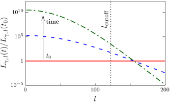
Figure 5: Luminosity distribution over angular harmonics $L_{\gamma,\,l}(t)$. We consider resonant emission from the stationary Bose star with ${M_{s}=1.36\,M_{s,\,0}}$, ${mR_{s}\sim M_{pl}^{2}/(mM_{s})\approx 115}$, and $g_{4}=0$. Lines are the fixed-time sections of luminosity in full numerical simulation.

In Appendix A we perform spherical decomposition of the electromagnetic field inside a Bose star. We find the same leading-order equations (16) in every angular sector $(l,\,m^{\prime})$, with dependence on $l$ emerging as an $O(mR_{s})^{-1}$ correction to the spatial derivatives

$$\partial_{z}\to\partial_{z}+\frac{il(l+1)}{mz^{2}}\;,$$ (42)

where $z=\pm r$, cf. Eq. (18). In fact, even this correction can be absorbed by the singular redefinition ${c_{i}^{\pm}\to c_{i}^{\pm}\exp[il(l+1)/mr]}$ of the electromagnetic amplitudes. Then the effect of angular quantum number is parametrically weaker than $(mR_{s})^{-1}$, with leading contribution coming from a small vicinity of ${r=0}$. We conclude that spherical modes with essentially different $l$ satisfy almost the same equations inside the star and grow at close rates $\mu_{l}\approx\mu$.

Our numerical simulation confirms this expectation, see Fig. 5. Namely, the numerical data suggest heuristic expression,

$$\mu_{l}-\mu\approx-0.034\,m\,l(l+1)\,\frac{M_{s}}{M_{s,0}}\,\left(\frac{mM_{s}}{M_{pl}^{2}}\right)^{3}\;,$$ (43)

where $\mu$ is approximately given by Eq. (35). Thus, dependence on $l$ is indeed an $O(mR_{s})^{-2}$ correction, see Appendix C.

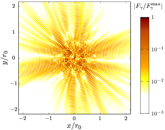
Figure 6: Electromagnetic flux $F_{\gamma}\equiv\boldsymbol{n}_{r}[\boldsymbol{E}\times\boldsymbol{H}]$ inside the resonating star from Fig. 5; $r_{0}=M_{pl}^{2}/(M_{s}m^{2})$. Interference between the waves moving in the $+r$ and $-r$ directions is clearly seen. The simulation uses random initial data to mimic quantum fluctuations in the electromagnetic vacuum, see Appendices D, E for details.

Now, it is explicit that all modes with

$$l\lesssim l_{\mathrm{cutoff}}\approx 2.4\,\left(\frac{M_{s}}{M_{s,\,0}}-1\right)^{1/2}\,\frac{M_{s,\,0}M_{pl}^{2}}{mM_{s}^{2}}\sim mR_{s}$$

grow simultaneously in resonance, see the vertical dotted line in Fig. 5. If the instability starts from random quantum fluctuations, it produces chaotic angular distribution in Fig. 6 with typical angular size $l_{\mathrm{cutoff}}^{-1}$. If the instability starts due to ambient radiowave, the cutoff sets typical width of the resonance beam.

IV.6 Two axion stars

Suppose two Bose stars came close to each other with negligible relative velocity. Together, their profiles may satisfy the resonance condition even if the individual stars are far away from it. Then strong and efficient parametric resonance may develop in this system Hertzberg:2018zte .

We describe this case considering the background

$$\psi=\psi_{s}({\bf x})\,\mathrm{e}^{i\theta_{s}}+\psi_{s}^{\prime}({\bf x})\,\mathrm{e}^{i\theta_{s}^{\prime}}\;,$$ (44)

of well separated static Bose stars $\psi_{s}$ and $\psi_{s}^{\prime}$ centered at $z=0$ and $z=L$, respectively. In Eq. (44) we explicitly introduced complex phases of stars $\theta_{s}$ and $\theta_{s}^{\prime}$.

Equations (16) can be solved analytically in the limit when the interstar distance is much larger than their sizes, $L\gg R_{s}$. In this case $\mu\sim O(L)^{-1}$ corresponds to the inverse light-crossing time between the stars. Outside every star i.e. at $z\ll L$ and at $z\gg 0$, we obtain

$$\left.\begin{array}[]{l}\displaystyle c_{x}^{+}=A\,\mathrm{e}^{\mu z}\,\cos D(z)\\[2.00749pt] c_{y}^{-}=-iA\,\mathrm{e}^{i\theta_{s}-\mu z}\sin D(z)\end{array}\right\}\;\mbox{outside $\psi_{s}^{\prime}$},$$ (47)

$$\left.\begin{array}[]{l}c_{x}^{+}=A^{\prime}\,\mathrm{e}^{\mu(z-L)}\,\sin[D^{\prime}_{\infty}-D^{\prime}(z)]\\[2.00749pt] c_{y}^{-}=-iA^{\prime}\,\mathrm{e}^{i\theta_{s}^{\prime}-\mu(z-L)}\cos[D^{\prime}_{\infty}-D^{\prime}(z)]\end{array}\right\}\;\mbox{outside $\psi_{s}$},$$ (50)

where $D$ and $D^{\prime}$ are computed using $\psi_{s}$ and $\psi_{s}^{\prime}$ in Eqs. (30), (31). Indeed, expressions (47) satisfy the boundary value problem inside the left and right stars with $O(\mu)$ precision, and both of them give correct solution between the stars. Gluing $c_{x}^{+}$ and $c_{y}^{-}$ in the latter region, one finds $A=A^{\prime}\mathrm{e}^{-\mu L}\sin D^{\prime}_{\infty}/\cos D_{\infty}$ and

$$\mu=\frac{1}{2L}\left[i\theta_{s}-i\theta_{s}^{\prime}+\ln\;\frac{\sin D_{\infty}\,\sin D^{\prime}_{\infty}}{\cos D_{\infty}\,\cos D^{\prime}_{+\infty}}\right]\;,$$ (51)

which confirms that $\mu\sim O(L)^{-1}$.

Expression (51) deserves discussion. First, the two-star system hosts parametric resonance if $\mathrm{Re}\,\mu\geq 0$ or $D_{\infty}+D^{\prime}_{\infty}\geq\pi/2$. This condition reproduces the naive criterion (31) with $\psi\to|\psi|$. Second, the resonance develops at a very slow rate $\mu\sim L^{-1}$ which is nevertheless much faster than the evolution of $\psi$ if $\mu\gg\omega_{s}$ or $mR_{s}^{2}\gg L$.

Third and importantly, left- and right-moving parametric waves have slightly different frequencies ${\omega_{\gamma}=m/2\pm\mathrm{Im}\,\mu}$, where $\mathrm{Im}\,{\mu}=(\theta_{s}-\theta_{s}^{\prime})/2L$, cf. Eq. (15). This splitting is a benchmark effect of incoherent axions. Technically, it appears because the phases of the resonant amplitudes are locally related to the phase of the axion field,

$$\arg\,c_{x}^{+}\approx\arg c_{y}^{-}-\mathrm{arg}\,\psi+\pi/2\;.$$ (52)

Indeed, all coefficients in Eqs. (16) become real after substitution $c_{y}^{-}\to ic_{y}^{-}\exp(i\,\mathrm{arg}\,\psi)$ with corrections suppressed by $\partial_{z}\,\mathrm{arg}\,\psi$; hence (52). In the above setup with two axion stars the shifts of emission frequencies ensure Eq. (52) inside each star at $z\approx 0$ and $L$.

Notably, one does expect formation of gravitationally bound groups of Bose stars in the QCD axion cosmology. Indeed, in the post-inflationary scenario these objects emerge in the centers of miniclusters which are organized in chains and hierarchically bound structures Vaquero:2018tib ; Buschmann:2019icd ; Eggemeier:2019khm . Once several stars within one group align with small relative velocities $v\ll(mL)^{-1}$, condition (31) may be satisfied and the parametric explosion follows. The spread of the produced spectrum will be $\delta\omega_{\gamma}/\omega_{\gamma}\sim L^{-1}$ due to random phases of the stars, even if their velocities are negligibly small.

V Diffuse axions

Our eikonal system (16) is a microscopic Maxwell’s equation in disguise. It is valid for general axion backgrounds including virialized distributions in the galaxy cores and axion miniclusters. In the latter cases, however, kinetic approach is simpler.

In this Section we study parametric radio-amplification in a cloud of random classical waves representing incoherent or partially coherent axions. We fix correlators

$$\langle\psi\rangle=0\;,\;\;\langle\psi^{*}(z)\psi(z^{\prime})\rangle=\rho\;C(z-z^{\prime})/(mf_{a})^{2}\;,$$ (53)

where $\rho$ is density, $C(0)=1$, and the correlation length is $\lambda=\int dy\,C(y)$.

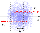
(a)                                     (b)

Figure 7: (a) Radiowaves going through a small region with axions. (b) Two resonant radiofluxes in a large axion cloud.

Let us coarse-grain Eqs. (16) to a kinetic equation in the stationary case. To this end we consider two radiowaves with fixed frequency $\omega_{\gamma}=m/2$ and amplitudes $A^{\pm}$ traveling back-to-back through a small axion region in Fig. 7a. This fixes the boundary conditions,

$$\left.c^{+}_{x}\right|_{z\to+\infty}=A^{+}\;,\qquad\left.c^{-}_{y}\right|_{z\to-\infty}=A^{-}\;,$$ (54)

and the incoming fluxes $F_{\gamma,\,in}^{\pm}=\mp m^{2}|A^{\pm}|^{2}/2$.

We assume that by itself, the axion region is too small to host a resonance. Then the nonrelativistic equations (16), (54) can be solved perturbatively,

$$c_{x}^{+}=A^{+}\left[1+D_{2,\,\infty}-D_{2}(z)\right]+iA^{-}\left[D_{\infty}^{*}-D^{*}(z)\right]\;,$$

$$c_{y}^{-}=A^{-}\left[1+D_{\infty}^{*}D(z)-D_{2}^{*}(z)\right]-iA^{+}D(z)\;,$$ (55)

where $D(z)$ is given by Eq. (31) and

$$D_{2}(z)={g^{\prime}m}\int_{-\infty}^{z}dz^{\prime}\,\psi^{*}(z^{\prime})\,D(z^{\prime})\;.$$ (56)

We compute the outgoing fluxes by performing ensemble average via Eq. (53),

$$F_{\gamma,\,out}^{+}=-\frac{m^{2}}{2}\langle|c_{x}^{+}|^{2}\rangle_{z\to-\infty},\;F_{\gamma,\,out}^{-}=\frac{m^{2}}{2}\langle|c_{y}^{-}|^{2}\rangle_{z\to+\infty}.$$

The solution (55) gives,

$$F_{\gamma,\,out}^{\pm}=F_{\gamma,\,in}^{\pm}(1+\mu_{\infty}^{\prime}L)-\mu_{\infty}^{\prime}L\,F_{\gamma,\,in}^{\mp}\;.$$ (57)

Here $L$ is the size of the axion region and ${\mu_{\infty}^{\prime}=\langle|D_{\infty}|^{2}\rangle/L}$ is the naive growth exponent in the infinite axion gas. The latter parameter is explicitly computed by assuming that the region is macroscopic, $L\gg\lambda$, and yet, small at the scales of $\rho$,

$$\mu_{\infty}^{\prime}=g_{a\gamma\gamma}^{2}\rho\lambda/8\;,$$ (58)

where we restored the physical coupling $g_{a\gamma\gamma}$.

Now, consider large axion cloud. We divide into small regions of width $L$, see Fig. 7b. Since equation (57) is valid in every region, we find,

$$\partial_{z}F_{\gamma}^{\pm}=\mu_{\infty}^{\prime}(z)(F_{\gamma}^{-}-F_{\gamma}^{+})\;,$$ (59)

where $F_{\gamma}^{\pm}(z)$ are the fluxes $F_{\gamma,\,in}^{\pm}\approx F_{\gamma,\,out}^{\pm}$ at the macroscopic position $z$.

Recalling that $F_{\gamma}^{+}$ and $F_{\gamma}^{-}$ travel in $-z$ and $+z$ directions, respectively, one restores the time derivative in Eq. (60) by changing

$$\partial_{z}F^{\pm}\to(\partial_{z}\mp\partial_{t})F^{\pm}\;.$$ (60)

After that our kinetic equation coincides with the one in Refs. Tkachev:1987cd ; Caputo:2018vmy if one trades the correlation length $\lambda(z)$ in Eq. (58) for the axion velocity ${v\sim(m\lambda)^{-1}}$ or spectral width of radiowaves $\delta\omega_{\gamma}\sim\lambda^{-1}$.

Solving Eq. (59) in the stationary case, we find,

$$F_{\gamma}^{-}(z)=F_{\gamma}^{+}(z)+F_{0}=F_{0}\int\limits_{-\infty}^{z}\mu_{\infty}^{\prime}(z^{\prime})\,dz^{\prime}\;,$$ (61)

where $F_{0}$ is the integration constant. Note that this solution does not indicate exponential growth of fluxes, unlike the time-dependent solutions of Eqs. (59), (60) behaving like $F^{\pm}_{\gamma}\propto\exp(\mu^{\prime}_{\infty}t)$ in the infinite medium.

Nevertheless, one can use Eq. (61) for waves with ${\omega_{\gamma}=m/2}$ ($\mu=0$) in two important respects. First, $\mu=0$ when the resonance is about to appear. In this case the ambient fluxes are absent: $F_{\gamma}^{+}(+\infty)=F_{\gamma}^{-}(-\infty)=0$, cf. Eq. (17). The solution (61) satisfies this criterion only at $D_{\infty,\,\mathrm{diff}}=1$, i.e. at the boundary of the region

$$D_{\infty,\,\mathrm{diff}}\equiv\frac{g_{a\gamma\gamma}^{2}}{8}\int_{-\infty}^{+\infty}\rho(z)\lambda(z)\,dz\geq 1\;.$$ (62)

This inequality gives precise condition for the parametric resonance in diffuse axions, cf. Eq. (31).

Second, even far away from the parametric instability Eq. (61) predicts amplification of ambient radioflux $F_{\gamma,\,in}=F^{+}(+\infty)$ due to decay of axions,

$${F_{\gamma,\,out}=F_{\gamma,\,in}\,/(1-D_{\infty,\,\mathrm{diff}})}\;,$$

where $F_{\gamma,\,out}=F^{+}(-\infty)$, cf. Sec. IV.4.

VI Moving axions

VI.1 Doppler shifts and new resonance condition

We just saw that motion of diffuse axions decreases their correlation length $\lambda\sim(mv)^{-1}$ and hence suppresses the resonance, cf. Eq. (62). In this Section we study the effect of moving coherent axions.

Let us rewrite the system (16) in terms of physical parameters: axion velocity $v_{i}(t,\,{\bf x})$ in Eq. (27), and density $\rho(t,\,{\bf x})=m^{2}f_{a}^{2}|\psi|^{2}$. To this end we change variables,

$$c_{x}^{+}=\tilde{c}_{x}^{+}\,\mathrm{e}^{-i\mathrm{arg}\,\psi/2}\;,\qquad c_{y}^{-}=\tilde{c}_{y}^{-}\,\mathrm{e}^{i\mathrm{arg}\,\psi/2}\;.$$ (63)

Eikonal equations take the form,

$$\left(2\mu+im\,v_{z}\right)\tilde{c}^{+}_{x}=2\partial_{z}\tilde{c}^{+}_{x}+ig_{a\gamma\gamma}(\rho/2)^{1/2}\;\tilde{c}^{-}_{y}\;,$$ (64a)

$$\left(2\mu+im\,v_{z}\right)\tilde{c}^{-}_{y}=-2\partial_{z}\tilde{c}^{-}_{y}-ig_{a\gamma\gamma}(\rho/2)^{1/2}\;\tilde{c}^{+}_{x}\;.$$ (64b)

Note that only a projection $v_{z}$ of the axion velocity to the resonance axis matters.

If $v_{z}$ is constant, one can eliminate it from Eqs. (64) by changing $\mu\to\mu-imv_{z}/2$. This is the Doppler shift of frequencies ${\omega_{\gamma}=m/2\pm\mathrm{Im}\,\mu}$ for the left- and right- moving waves in Eq. (13). Apart from that, constant velocities do not affect the resonance at all. Indeed, one can always transform to the rest frame of axions.

The situation changes if some parts of the axion matter move with respect to others: ${v_{z}=v_{z}(z)}$. Then the axions decaying in various parts produce photons with different frequencies, and this kills Bose amplification of induced decays. Thus, relative velocities are the main show-stoppers for the parametric resonance.

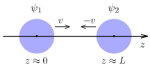
Figure 8: Two moving Bose stars.

In the next Section we will demonstrate that only the coherent regions with relative velocities

$$v\lesssim(mR)^{-1}\;,$$ (65)

can be simultaneously in resonance, where $R$ is the size of these regions. The above expression is natural. Indeed, $R^{-1}$ is the momentum spread in the resonance mode. If the Doppler shift $mv$ is larger, photons produced in different regions are out of resonance.

VI.2 Two moving axion stars

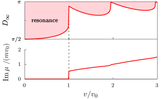
Figure 9: Condition for parametric resonance in two moving axion stars (top panel) and respective Doppler shift $\mu^{\prime}=\mathrm{Im}\,\mu$ (bottom panel).

To get a qualitative understanding of relative velocities, we consider two identical Bose stars approaching each other at a nonrelativistic constant speed $v$,

$$\psi=\psi_{1}(z)\,\mathrm{e}^{imvz}+\psi_{2}(z)\,\mathrm{e}^{-imv(z-L)}\;,$$

see Fig. 8. For simplicity we will assume that $\psi_{1}$ and $\psi_{2}$ are equal to a constant $\psi_{0}$ in the regions $0<z<2R_{s}$ and ${L<z<L+2R_{s}}$, and they are zero outside. We are going to find out whether this configuration develops a resonance before the merger i.e. when the profiles of the stars still do not overlap.

We compute the resonant mode by solving Eqs. (64) in the regions of constant $\rho$, $v_{z}$ and gluing the original amplitudes $c_{x,y}^{\pm}$ at $z=2R_{s}$ and $z=L$. Then the boundary conditions (17) give equation for the growth exponent $\mu$. At the border of resonance ${\mu=i\mu^{\prime}}$ becomes imaginary and the equation simplifies,

$$\mathrm{tan}^{2}(2\kappa_{-}R_{s})\mathrm{tan}^{2}(2\kappa_{+}R_{s})=\left[1+\frac{(2\mu^{\prime}-mv)^{2}}{m^{2}v_{0}^{2}\cos^{2}(2\kappa_{-}R_{s})}\right]\\ \times\left[1+\frac{(2\mu^{\prime}+mv)^{2}}{m^{2}v_{0}^{2}\cos^{2}(2\kappa_{+}R_{s})}\right]\;.$$ (66)

Here we introduced the relevant velocity scale ${v_{0}=2g^{\prime}\psi_{0}}$ and notations $4\kappa_{\pm}^{2}=m^{2}v_{0}^{2}+(2\mu^{\prime}\pm mv)^{2}$.

At a very naive level, one may use $|\psi|$ instead of $\psi$ in Eq. (31). Then the resonance is expected at ${D_{\infty}\equiv 4g^{\prime}m\psi_{0}R_{s}\geq\pi/2}$, where $D_{\infty}$ sums up contributions from both stars. In truth, the solution of Eq. (66) exists only in the shaded region in Fig. 9 (top panel). The Doppler shift $\mu^{\prime}=\mu^{\prime}(v)$ at the boundary of this region is plotted in the bottom panel.

One observes sharp first-order phase transition at ${v\approx v_{0}}$ between the two resonance regimes, see the vertical dashed line in Fig. 9. At $v<v_{0}$ the Doppler shift is absent, $\mathrm{Im}\,\mu=0$, although the stars have nonzero velocities. Besides, the naive resonance condition $D_{\infty}\geq\pi/2$ is approximately valid indicating that the instability develops simultaneously in both stars. To the contrary, at $v>v_{0}$ two individual stars host their own resonances, with little help from each other. In this case the Doppler shift is $\mathrm{Im}\,\mu\approx mv/2$ and the resonance condition $D_{\infty}/2>\pi/2$ coincides with that for one star. We conclude that the two-star resonance occurs only at $v\leq v_{0}$ or Eq. (65).

Note that the phase transition in Fig. 9 can be understood analytically. At large relative velocities ${v\gg v_{0}}$ at least one of the two brackets in the right-hand side of Eq. (66) should be small, so the solutions are ${\mu^{\prime}\approx\pm mv/2}$ and $2\kappa_{\pm}R_{s}\approx D_{\infty}/2\approx\pi/2$. This corresponds to resonance in individual stars. At $v\lesssim v_{0}$ Eq. (66) with $\mu^{\prime}=0$ takes the form

$$\cos(4\kappa_{\pm}R_{s})=-v^{2}/v_{0}^{2}\;,$$

where $\kappa_{\pm}=m(v_{0}^{2}+v^{2})^{1/2}/2$. At ${v\ll v_{0}}$ we obtain ${D_{\infty}=\pi/2}$, — a condition for the two-star resonance. At $v>v_{0}$ the above equation in the case $\mu^{\prime}=0$ does not have solutions.

VI.3 Collapsing stars

(a)                              (b)

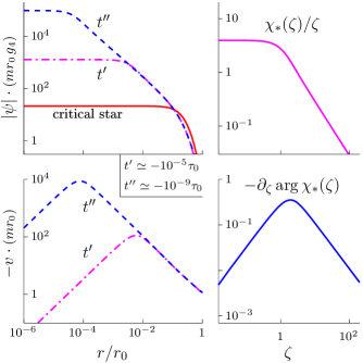
Figure 10: (a) Numerical solution to the Schrödinger-Poisson system (6), (7) describing collapse of a critical Bose star; the axion velocity is $v=m^{-1}\,\partial_{r}\mathrm{arg}\,\psi$. We use space and time units ${r_{0}=g_{4}M_{pl}/(mf_{a})}$ and $\tau_{0}=mr_{0}^{2}$, see Appendix C. (b) Universal self-similar attractor.

Now, consider collapse of a critical axion star, ${M_{s}=M_{cr}}$, caused by the attractive self-interaction of axions. During this process the axions fall into the star center acquiring velocities and making the density grow, see Fig. 10a. These two effects suppress the resonance and support it, respectively.

We are going to study the resonance at the first stage of the collapse when the infalling axions are still nonrelativistic and their field is weak, $|\psi|\ll 1$. In this case the Schrödinger-Poisson system (6), (7) for axions is applicable, whereas the electromagnetic field is described by Eqs. (16).

Figure 11: (a) Electromagnetic coupling $g_{a\gamma\gamma}$ required for parametric resonance in collapsing critical star at the moment when its core radius is $r_{c}(t)$. (b) Doppler shifts $\pm\mathrm{Im}\,\mu$ at the moment of ignition. Unit of length is ${r_{0}=g_{4}M_{pl}/(mf_{a})}$.

To find out how the parametric instability progresses, we numerically solve the boundary value problem (16) in the background $\psi(t,\,r)$ of the collapsing star at every $t$. We characterize the stage of collapse with the radius ${r=r_{c}(t)}$ where the axion field drops by a factor of two from its value in the center: ${|\psi(t,\,r_{c}(t))|=|\psi(t,\,0)|/2}$. We will see that the region $r\lesssim r_{c}$ is important for the resonance despite the fact that $r_{c}(t)$ decreases by orders of magnitude during collapse. Shaded region Fig. 11a covers couplings $g_{a\gamma\gamma}$ required for the resonant solutions of Eqs. (16) to exist at time $r_{c}(t)$. At the lower boundary of this region $\mathrm{Re}\,\mu=0$; the respective Doppler shifts $\mathrm{Im}\,\mu$ are presented in Fig. 11b.

Since the star is spherically-symmetric, ${\psi(z)=\psi(-z)}$, the photon modes with complex exponents $\mu$ appear in conjugate pairs. Indeed, for every solution $\{c_{x}^{+}(z),\,c_{y}^{-}(z)\}$ of Eqs. (16) with eigenvalue $\mu$, there exists a solution $\{[c_{y}^{-}(-z)]^{*},\,[c_{x}^{+}(-z)]^{*}\}$ with eigenvalue $\mu^{*}$. Physically, this means that for every axion there exists a diametrically opposite axion with the opposite velocity giving Doppler shift $-\mathrm{Im}\,\mu$. Two signs in the ordinate label of Fig. 11 represent these two solutions.

In Fig. 11 we again see the first-order phase transition (vertical dashed line) described in Sec. VI.2. Indeed, if the resonance appears immediately after the collapse begins (large $r_{c}$), it involves all slowly-moving axions and develops with $\mathrm{Im}\,\mu=0$. At later stages of collapse (smaller $r_{c}$) the resonance can be supported only by fast axions in the dense star core, hence the Doppler shift $\mathrm{Im}\,\mu\neq 0$. Importantly and unlike in the previous Section, the stage with fast axions is better for resonance, as it can occur at smaller couplings, cf.  Figs. 11a and 9.

We therefore consider resonance in the central core of a collapsing star. It was shown Zakharov12 ; Levkov:2016rkk that evolution of the axion field in this region is described by the universal self-similar attractor,

$$\psi(t,r)=\frac{(-mt)^{-i\omega_{*}}}{mrg_{4}}\chi_{*}\left(\zeta\right)\;,\qquad\zeta=r\,\sqrt{-m/t}\;,$$ (67)

where $t<0$, $\omega_{*}\approx 0.54$ and the function $\chi_{*}(\zeta)$ is presented in Fig. 10b. The core size $r_{c}(t)\approx 1.5\,(-t/m)^{1/2}$ shrinks from the macroscopic values $r_{c}\sim R_{s}$ to $m^{-1}$ during self-similar stage. Without the parametric resonance into photons, relativistic corrections become relevant Levkov:2016rkk at the end of this stage $t\gtrsim-m^{-1}$. Simultaneously, the weak–field approximation gets broken and higher-order terms of the axion potential (3) become essential. Below we concentrate on the situations when the resonance starts at the nonrelativistic stage $t\ll-m^{-1}$.

Substituting Eq. (67) into the spectral problem (16) and changing variables $c^{\pm}=(-mt)^{\pm i\omega_{*}/2}\,\tilde{c}^{\pm}(\zeta)$, we arrive to time-independent spectral problem

$$\tilde{\mu}\tilde{c}_{x}^{+}=\partial_{\zeta}\tilde{c}_{x}^{+}+\frac{ig^{\prime}}{g_{4}}\,\frac{[\chi_{*}(\zeta)]^{*}}{\zeta}\,\tilde{c}_{y}^{-}\;,$$ (68a)

$$\tilde{\mu}\tilde{c}_{y}^{-}=-\partial_{\zeta}\tilde{c}_{y}^{-}-\frac{ig^{\prime}}{g_{4}}\,\frac{\chi_{*}(\zeta)}{\zeta}\,\tilde{c}_{x}^{+}\;,$$ (68b)

which involves only one combination of parameters $g^{\prime}/g_{4}$. We also introduced

$$\mu=\tilde{\mu}\,\sqrt{-m/t}\;,$$ (69)

where the spectral parameter $\tilde{\mu}$ does not depend on time. We extend the above equations to the full star diameter $-\infty<\zeta<+\infty$ with $\chi_{*}(-\zeta)=-\chi_{*}(\zeta)$, as explained in Appendix A.

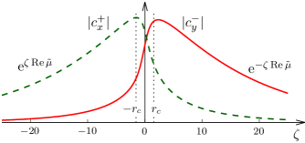
Figure 12: Resonance mode in the collapsing star; functions $c_{x}^{+}(\zeta)$ and $c_{y}^{-}(\zeta)$ are not symmetric to each other. We use self-similar coordinate $\zeta$ and $g_{a\gamma\gamma}=0.37\,g_{4}/f_{a}$. The respective eigenvalue is $\tilde{\mu}\approx 0.065+0.025\,i$.

We numerically solve Eqs. (68) with boundary conditions (17); the exemplary solution at $g^{\prime}/g_{4}\approx 0.13$ is shown in Fig. 12. Notably, the nontrivial part of this solution has width corresponding to $r_{c}(t)$ (vertical lines in Fig. 12). Beyond this part $|c_{i}^{\pm}|$ freely decay as $\exp\{-|\zeta|\,\mathrm{Re}\,\tilde{\mu}\}$. Thus, the resonance mode shrinks on par with the collapsing star.

Numerical solutions of Eqs. (68), exist only at

$$g_{a\gamma\gamma}\geq 0.25\,\frac{g_{4}}{f_{a}}\;.$$ (70)

This is a general condition to ignite parametric instability in collapsing stars. It reproduces minimal coupling required for the resonance in Fig. 11 (horizontal dashed line). Also, it is twice weaker than the condition for critical stars before collapse, cf. Eq. (33). For QCD axions, the region (70) is above the dashed line in Fig. 2.

Figure 13: Rescaled growth exponents $\tilde{\mu}$ in the collapsing star.

If the above inequality is met, the resonance progresses with two complex time-dependent exponents $\mu$ and $\mu^{*}$ in Eq. (69), where $\pm\mathrm{Im}\,\mu$ are the Doppler shifts. The respective eigenvalues $\tilde{\mu}$ are plotted in Fig. 13. Importantly, the time dependence of $\mu$ does not stop the resonance. Indeed, we already argued that the respective mode behaves like a localized level in quantum mechanics. Slow variations of external background do not change occupation of this level if the adiabatic condition is satisfied,

$$\frac{\partial_{t}\mu}{\mu^{2}}\sim(-mt)^{-1/2}\ll 1\;.$$ (71)

Thus, the electromagnetic field sits on two quasi-stationary resonance levels,

$$C_{\alpha}^{\pm}=A\,c_{\alpha}^{\pm}(t,\,z)\,\mathrm{e}^{\int_{t_{0}}^{t}dt\,\mu}\pm A^{\prime}\,\epsilon_{\alpha\beta}\,[c_{\beta}^{\mp}(t,\,-z)]^{*}\,\mathrm{e}^{\int_{t_{0}}^{t}dt\,\mu^{*}},$$

at least until the backreaction ruins the self-similar background.

Figure 14: Luminosity (72) of parametric emission from the collapsing star in Fig. 10a at $g_{a\gamma\gamma}=0.33\,g_{4}/f_{a}$, $b=0.9$, and $\varphi_{0}=0$. Self-similar result (69) (dashed line) is compared to the direct solution of Eqs. (16) (points).

The axion star radio-luminosity follows from the above representation. Interestingly, it oscillates in time due to interference between the modes,

$$L_{\gamma}\propto\mathrm{e}^{2\mathrm{Re}\int_{t_{0}}^{t}\mu\,dt}\left[1+b\,\cos\left(2\mathrm{Im}\int_{t_{0}}^{t}\mu\,dt+\varphi_{0}\right)\right],$$ (72)

where $b$ and $\varphi_{0}$ depend on the initial amplitudes $A$, $A^{\prime}$, with $b=1$ representing equipartition. In Fig. 14 we illustrate these oscillations at $b=0.9$, $\varphi_{0}=0$. Dashed line in this figure represents self-similar formula with $\int\mu\,dt=-2\tilde{\mu}(-mt)^{1/2}$. It coincides with the direct result (points) obtained by solving Eqs. (16) for $\mu(t)$ numerically in the background of a collapsing star and then using Eq. (72). This supports our analytic solution in Eq. (69).

Figure 15: Luminosity $L_{\gamma}(t)$ of critical collapsing star during parametric resonance; $g_{a\gamma\gamma}=0.33\,g_{4}/f_{a}$. Full numerical simulation (solid line) is compared to the solution of Eqs. (16) (points). We use universal units from Appendix C; in particular, $\psi_{0}^{2}=10^{3}\,(f_{a}/g_{4}^{2}M_{pl})^{2}$.

To test the above picture of parametric resonance during collapse, we simulate the coupled system of relativistic equations (10), (21) for photons and axions, see Fig. 15, movie movie , and Appendix E for details. We find that at first, the star squeezes with no effect on the electromagnetic field. But once the localized solution of Eqs. (16) appears, growth and oscillations of the luminosity begin (solid line in Fig. 15). The exact result is reproduced by Eq. (72) (points), where $\mu(t)$ is obtained by solving the boundary value problem (16) and $b$, $\phi_{0}$ are obtained from the fit.

It is worth reminding that Eq. (72) is applicable only for nonrelativistic stars deep in the self-similar regime. This is possible only at very large values of $mR_{s}$ which are hard to achieve in relativistic simulations. In particular, the value of $\mu$ in Eq. (69) is by a factor of two different from the simulation in Fig. 15.

We finish this Section with a mystery. Figure 15 demonstrates that once the inequality (37) is broken (shaded region), the backreaction ruins self-similar dynamics. Indeed, the axion field does not behave anymore as $|\psi(t,\,0)|^{-2}\propto-t$, like Eq. (67) suggests. Nevertheless, the luminosity continues to grow and saturates only deep inside the backreaction region. We will investigate this nonlinear regime in the forthcoming publication Levkov .

For QCD axions, the saturated luminosity in Fig. 15 is,

$$L_{\gamma}=1.5\cdot 10^{41}\left(\frac{m}{26\,\mu\mathrm{eV}}\right)^{-3}{\rm erg}\cdot{\rm s}^{-1}\;,$$ (73)

while the corresponding flux strongly depends on direction, see Fig. 6. Notably, this is close to the parameters of Fast Radio Bursts, $L_{\mathrm{FRB}}=10^{38}-10^{40}\,\mathrm{erg}\cdot\mathrm{s}^{-1}$.

VII Discussion

In this paper we have found that the finite-volume parametric resonance is described by the quasi-stationary Schrödinger-like system (16) with non-Hermitean “Hamiltonian.” That is where the fun has begun! Photon instability modes became localized states, and their growth exponents ${\mathrm{Re}\,\mu>0}$ — eigenvalues of the “Hamiltonian.” The condition for the resonance then indicates whether the localized states exist. Using this technique, we computed the resonance condition for the isolated Bose stars, collapsing and moving stars, their groups, and diffuse axions. We argued that axions with relative velocities exceeding a certain value of order $(mR)^{-1}$, are sharply out of resonance, where $R$ is the system size.

With help of quantum-mechanical perturbation theory, we analytically computed the instability modes and growth exponents in the physically motivated case of slow resonance, $\mu R\ll 1$. Interestingly, our theory predicts a long-living quasi-stationary photon mode with small negative decay exponent $\mathrm{Re}\,\mu<0$ after the resonance switches off, and we see this mode in simulations.

We have found two unexpected applications of our method. First, it describes stimulated emission of ambient radiation in axion stars. We observed that these objects can realistically give larger contribution to the radiobackground than the diffuse axions, producing a thin spectral line at $\omega_{\gamma}\approx m/2$. Second, with additional coarse-graining our approach reproduces well-known kinetic equation for photons interacting with virialized axions.

A warning is in order: our technique is applicable only in the case of nonrelativitic axions at high occupation numbers. These approximations may break down only under extreme conditions, say, in the strong gravitational field of a black hole or a neutron star, or at very late stages of Bose star collapse. That is why our method should work in vast majority of astrophysical settings with dark matter axions, and we expect that truly cool applications are still ahead. Besides, astrophysics offers an impressive set of situations where the resonance condition can be satisfied, and the ones with the largest $D_{\infty}$ are of primary interest. Using our method, one can study parametric instability in superradiant axion clouds near rotating black holes Rosa:2017ury , or in tidally elongated axion stars falling onto the neutron stars Tkachev:2014dpa , or in groups of gravitationally bound Bose stars Hertzberg:2018zte . In all these cases an observable radio-flash can appear, constraining the axion models or even explaining Fast Radio Bursts Petroff:2019tty . On the calmer side, objects at the rim of parametric resonance can give large contributions into the radiobackground possibly explaining ARCADE 2 Fixsen:2009xn and EDGES Bowman:2018yin anomalies.

Technically, we completely disregarded potentially important light-bending and divergence effects of the resonance rays, cf. Blas:2019qqp ; McDonald:2019wou , as well as phenomena of astrophysical plasma. These certainly deserve a separate study.

We explicitly saw that gravitational and self-interaction energies of axions inside the star trivially shift the photon frequencies without affecting the resonance. We do not expect these effects to be important in other situations as well. In particular, the distribution function of virialized axions in the galaxy depends on their total energy $E$, not kinetic or potential. The photon of frequency $\omega_{\gamma}\approx E/2$ will stay in resonance with same part of the ensemble in different parts of the galaxy Tkachev:1987cd ; Riotto:2000kh . Thus, the main show-stoppers for the parametric instabilities are the Doppler shifts and backreaction effects.

Appendix A Spherically-symmetric case

In the background of a spherical axion star with ${\psi=\psi(t,\,r)}$ it is natural to decompose the electromagnetic field $\boldsymbol{A}=\{A_{i}\}$ into spherical harmonics,

$$\boldsymbol{A}=\sum_{lm^{\prime}}\left(A_{Y}^{lm^{\prime}}\boldsymbol{Y}_{lm^{\prime}}+A_{\Psi}^{lm^{\prime}}\boldsymbol{\Psi}_{lm^{\prime}}+A_{\Phi}^{lm^{\prime}}\boldsymbol{\Phi}_{lm^{\prime}}\right)$$ (74)

where we use the gauge $A_{0}=0$, spherical vectors ${\boldsymbol{Y}_{lm^{\prime}}=\boldsymbol{x}\,Y_{lm^{\prime}}/r}$, ${\boldsymbol{\Psi}_{lm^{\prime}}=r\boldsymbol{\nabla}\,Y_{lm^{\prime}}}$, ${\boldsymbol{\Phi}_{lm^{\prime}}=[\boldsymbol{\nabla}\times{\bf x}]\,Y_{lm^{\prime}}}$, and denote the standard spherical functions by $Y_{lm^{\prime}}(\theta,\,\phi)$. Below we omit the superscripts $lm^{\prime}$ for brevity.

The coefficients of decomposition $A_{Y,\Psi,\Phi}(t,\,r)$ depend only on time $t$ and radial coordinate $r$. Substituting Eq. (74) into the Maxwell’s equation (10), one finds the Gauss law

$$A_{\Psi}=\frac{\partial_{r}(r^{2}A_{Y})}{r\,l(l+1)}$$ (75)

and two dynamical equations

$$r^{2}\partial_{t}^{2}A_{Y}=\partial^{2}_{r}(r^{2}A_{Y})-l(l+1)A_{Y}$$ (76a)

$$\qquad\qquad\qquad\qquad\qquad-g_{a\gamma\gamma}\,l(l+1)(\partial_{t}a)\,rA_{\Phi}\;,$$

$$r\partial_{t}^{2}A_{\Phi}=\partial^{2}_{r}(rA_{\Phi})-l(l+1)\,A_{\Phi}/r$$ (76b)

$$\qquad\qquad\qquad\qquad-g_{a\gamma\gamma}\partial_{t}a\left[A_{Y}-\frac{\partial^{2}_{r}(r^{2}A_{Y})}{l(l+1)}\right]\;,$$

where we omitted terms with $\partial_{r}a$ because they are suppressed by extra powers of $(mr)^{-1}$ and will not contribute into equations for $C$’s.

We finally introduce the eikonal ansatz,

$$(mr)^{2}\,A_{Y}=2il(l+1)\left\{C_{Y}^{+}\mathrm{e}^{im(r+t)/2}\right.$$ (77)

$$\qquad\qquad\qquad\qquad\left.+C_{Y}^{-}\mathrm{e}^{im(r-t)/2}\right\}+\mathrm{h.c.}\;,$$

$$mr\,A_{\Phi}=C_{\Phi}^{+}\,\mathrm{e}^{im(r+t)/2}+C_{\Phi}^{-}\,\mathrm{e}^{im(r-t)/2}+\mathrm{h.c.}$$

Using it in the above equations and omitting the $(mr)^{-1}$ suppressed contributions, we find eikonal equations (14) at $z=r>0$ for the unknowns $(C_{Y}^{+},\,C_{\Phi}^{-})$ in place of $(C_{x}^{+},\,C_{y}^{-})$, with the additional term (42) representing derivatives with respect to the spherical angles: ${\Delta_{\theta\phi}=-l(l+1)}$. The pair $(C_{\Phi}^{+},\,-C_{Y}^{-})$ satisfies the same equations.

There are two subtleties in the spherically-symmetric case. First, the transverse polarizations $A_{\Phi}$ and ${A_{\Psi}\propto rA_{Y}}$ are proportional to $r^{-1}$, see Eqs. (75), (77). This introduces $r^{-2}$ falloff of the electromagnetic flux $F_{\gamma,\,out}$ at infinity and additional factors ${l(l+1)/(4\pi m^{2}r^{2})}$ in the backreaction terms of Eqs. (22), (24).

Second, proper boundary conditions should be imposed at ${r=0}$. Solving Eqs. (76) to the leading order at $r\ll R_{s}$, we find that $A_{\Phi}$ and $rA_{Y}$ are linear combinations of the Bessel spherical functions $j_{l}(mr/2)\exp\{\pm imt/2\}$. The $mr\gg 1$ asymptotics of the latter give boundary conditions

$$C_{Y}^{+}=(-1)^{l}\,(C_{Y}^{-})^{*}\;,\qquad C_{\Phi}^{+}=(-1)^{l+1}\,(C_{\Phi}^{-})^{*}$$

at $r=0$.

Importantly, there is no need to solve Eqs. (14) on the half-line $z=r>0$. Instead, we extend $C_{\alpha}^{\pm}$ to another half-line using $C_{x}^{+}(z)=(-1)^{l}\,[C_{Y}^{-}(-z)]^{*}$ and ${C_{y}^{-}(z)=(-1)^{l+1}\,[C_{\Phi}^{+}(-z)]^{*}}$ at $z=-r<0$. After that $C_{x}^{+}$ and $C_{y}^{-}$ satisfy Eqs. (14) along the entire star diameter $-\infty<z<+\infty$, and the boundary conditions at $r=0$.

Appendix B The spectrum of a symplectic operator

Consider the eigenvalue problem (16) at real $\psi$. We denote the $2\times 2$ operator in its right-hand side by

$$\hat{\cal L}=\begin{pmatrix}\partial_{z}&ig^{\prime}m\psi\\[4.015pt] -ig^{\prime}m\psi&-\partial_{z}\end{pmatrix}.$$ (78)

One can explicitly check that this operator is symplectic, i.e. satisfies

$$\hat{\Omega}\hat{\cal L}=\hat{\cal L}^{\dagger}\hat{\Omega},\qquad\mbox{where}\qquad\hat{\Omega}=\begin{pmatrix}0&-i\\ i&0\end{pmatrix}$$ (79)

is a symplectic form.

Now, suppose $|\xi\rangle=(c_{x}^{+},\;c_{y}^{-})^{T}$ is the eigenmode of $\hat{\cal L}$ satisfying the resonance boundary conditions (17). In this case the scalar product

$$\langle\xi|\hat{\Omega}|\xi\rangle=i\int dz\,\left(c_{y}^{-*}\,c_{x}^{+}-c_{x}^{+*}\,c_{y}^{-}\right)$$ (80)

converges; below we fix normalization ${\langle\xi|\hat{\Omega}|\xi\rangle=1}$. Then

$$\mu^{*}=\langle\xi|\hat{\Omega}\hat{\cal L}|\xi\rangle^{\dagger}=\langle\xi|\hat{\cal L}^{\dagger}\hat{\Omega}|\xi\rangle^{\dagger}=\mu\;,$$ (81)

where in the last equality we used Eq. (79). Thus, the localized resonance modes of $\hat{\cal L}$ satisfying (17) have real $\mu$.

Note that the eigenmodes of $\hat{\cal L}$ with different eigenvalues are orthogonal to each other in the sense of the scalar product (80). Indeed, repeating the computation (81) for eigenvectors $|\xi_{1}\rangle$ and $|\xi_{2}\rangle$ with exponents $\mu_{1}$ and $\mu_{2}$, we find

$$\mu_{2}^{*}\,\langle\xi_{1}|\hat{\Omega}|\xi_{2}\rangle^{\dagger}=\mu_{1}\,\langle\xi_{1}|\hat{\Omega}|\xi_{2}\rangle^{\dagger}\;,$$ (82)

which proves $\langle\xi_{1}|\hat{\Omega}|\xi_{2}\rangle=0$. Moreover, one can argue that the set of $\hat{\cal L}$ eigenmodes — the resonance ones and the ones from the continuum spectrum — forms complete basis in the space of bounded functions $c_{x}^{+}$ and $c_{y}^{-}$.

With the above definitions we can develop a perturbation theory for the spectrum of $\hat{\cal L}$. Indeed, suppose at $\psi=\psi_{0}(z)$ the operator $\hat{\cal L}=\hat{\cal L}_{0}$ has a normalized eigenmode $|\xi_{0}\rangle$ with zero eigenvalue, $\hat{\cal L}_{0}|\xi_{0}\rangle=0$. At slightly different $\psi=\psi_{0}(z)+\delta\psi(z)$ this operator receives variation $\delta\hat{\cal L}=-g^{\prime}m\,\delta\psi\,\hat{\Omega}$. In this case its resonance eigenmode $|\xi\rangle=|\xi_{0}\rangle+|\delta\xi\rangle$ is close to $|\xi_{0}\rangle$, and the respective eigenvalue $\mu$ is small. The eigenvalue problem $\hat{\cal L}|\xi\rangle=\mu|\xi\rangle$ takes the form,

$$\delta\hat{\cal L}|\xi_{0}\rangle+\hat{\cal L}_{0}|\delta\xi\rangle=\mu|\xi_{0}\rangle\;,$$ (83)

where we ignored quadratic terms in perturbations. The scalar product with $|\xi_{0}\rangle$ gives,

$$\mu=\frac{\langle\xi_{0}|\hat{\Omega}\delta\hat{\cal L}|\xi_{0}\rangle}{\langle\xi_{0}|\hat{\Omega}|\xi_{0}\rangle}=-{g^{\prime}m}\,\frac{\langle\xi_{0}|\delta\psi|\xi_{0}\rangle}{\langle\xi_{0}|\hat{\Omega}|\xi_{0}\rangle}$$ (84)

Using explicit solution (29) for $\xi_{0}$, we finally obtain

$$\mu={g^{\prime}m}\;\frac{\int dz\,\left[\psi(t,\,{\bf x})-\psi_{0}({\bf x})\right]}{\int dz\,\sin(2D_{0})}\;.$$ (85)

With (31) this expression reproduces Eq. (34) from the main text.

Appendix C Scaling symmetry

We calculate parameters of Bose stars using scaling symmetry of the Schrödinger-Poisson system (6), (7). Consider first the model without self-coupling, $g_{4}=0$. One finds that change of variables

$${\bf x}=\lambda\,\tilde{\bf x}\;, t=m\lambda^{2}\,\tilde{t}\;,$$ (86a)

$$\Phi=\frac{\tilde{\Phi}}{(m\lambda)^{2}}\;, \psi=\frac{M_{pl}\,\tilde{\psi}}{m^{2}\lambda^{2}f_{a}}$$ (86b)

with arbitrary $\lambda$ removes all constants from the equations. This scaling allows us to map the model with arbitrary parameters to a reference one with ${\tilde{\psi}(0)=1}$. We perform numerical calculations in tilded variables and then scale back to physical. Parameter $\lambda$ disappears in final answers, if one expresses it via the chosen Bose star characteristics, e.g. its mass,

$$M_{s}=m^{2}f_{a}^{2}\int d^{3}{\bf x}\,|\psi_{s}|^{2}=\tilde{M}_{s}\,\frac{M_{pl}^{2}}{\lambda m^{2}}\;,$$ (87)

where $\tilde{M}_{s}\approx 3.9$ is computed numerically. Similarly, the parameter (31) equals,

$$D_{\infty}\approx 0.80\,g_{a\gamma\gamma}\,\frac{M_{pl}}{\lambda m}\;.$$ (88)

Using this approach, we obtain Eqs. (32), (35).

In models with $g_{4}\neq 0$ the self-interaction can be ignored at $M\ll M_{cr}$, see Eq. (9), and we are back to the above situation. Stars with $M\geq M_{cr}$ are unstable. In the main text we mostly consider the critical star with ${M=M_{cr}}$. In this case one excludes all parameters from the equations using Eqs. (86) with $\lambda=g_{4}M_{pl}/mf_{a}$, computes the critical star numerically, and then restores the physical parameters. The integral (31) in this case equals

$$D_{\infty}\approx 3.04\;\frac{g_{a\gamma\gamma}f_{a}}{g_{4}}$$ (89)

implying (33). These “self-interaction” units are exploited in Figs. 10, 11, 14, 15.

Finally, if self-coupling is negligible but backreaction of photons on axions is relevant, all constants can be eliminated from Eqs. (16), (22), (7) using Eqs. (86), $C_{\alpha}^{\pm}=\tilde{C}_{\alpha}^{\pm}(M_{pl}/g_{a\gamma\gamma})^{1/2}(m\lambda)^{-2}$, $\mu=\tilde{\mu}/\lambda$, and ${\lambda=g_{a\gamma\gamma}M_{pl}/m}$. We perform this rescaling to plot universal quantities in Figs. 3, 4, and 15.

Appendix D Initial conditions

In real astrophysical settings the axion stars are embedded into the background of classical radiowaves which can give a good initial kick to the parametric instability, cf. Sec. IV.4. But this mechanism essentially depends on the environment, so outside of Sec. IV.4 we assume quantum start, i.e. the resonance set off by the spontaneous decays of axions inside the isolated star.

Detailed study of quantum evolution is beyond the scope of this paper, so we use a shortcut. Namely, the flux $F_{\gamma}\sim|\boldsymbol{E}|^{2}\sim|\boldsymbol{H}|^{2}$ of spontaneous photons can be estimated from energy conservation,

$$\partial_{t}M_{s}=-\Gamma_{a\gamma\gamma}M_{s}=-4\pi r^{2}F_{\gamma}\;,$$ (90)

where we assumed spherical Bose star and introduced the axion decay width $\Gamma_{a\gamma\gamma}=g_{a\gamma\gamma}^{2}m^{3}/64\pi$. This gives typical amplitudes

$$|\boldsymbol{E}|\sim|\boldsymbol{H}|\sim\frac{1}{R_{s}}\left(\frac{M_{s}\Gamma_{a\gamma\gamma}}{4\pi}\right)^{1/2}$$ (91)

of spontaneous emission.

It is worth reminding that the exponential growth of the resonance mode washes out all details of initial quantum evolution, with just one logarithmically sensitive parameter surviving: the time of growth. That is why the above order-of-magnitude description is adequate.

In numerical simulation of Appendix E we mimic the quantum bath of spontaneous photons using a stochastic ensemble of random classical waves with amplitudes (91). This is required only in dynamical situations such as the axion star collapse in Sec. VI.3.

Appendix E Full relativistic simulation

We test the theory by numerically evolving the equations (10) and (21) for the electromagnetic and axion fields. In computations we consider only spherically symmetric axion backgrounds, $a=a(t,\,r)$. This is justified at the linear stages of parametric resonance and should be valid at least qualitatively during backreaction. To make Eq. (21) self-consistent, we average its right-hand side over spherical angles: $F_{\mu\nu}\tilde{F}_{\mu\nu}\to\int d\Omega\,F_{\mu\nu}\tilde{F}_{\mu\nu}/4\pi$. We decompose electric and magnetic fields $E_{i}=F_{0i}$ and $H_{i}=-\epsilon_{ijk}F_{jk}/2$ in spherical harmonics $\boldsymbol{Y}_{lm^{\prime}}$, $\boldsymbol{\Psi}_{lm^{\prime}}$, and $\boldsymbol{\Phi}_{lm^{\prime}}$ introduced in Appendix A. With the cutoff $l\leq l_{max}$, we find $6l_{max}(l_{max}+2)+1$ equations for the same number of unknowns $E_{lm^{\prime}}^{Y,\,\Psi,\,\Phi}(t,\,r)$, $H_{lm^{\prime}}^{Y,\,\Psi,\,\Phi}(t,\,r)$, and $a(t,\,r)$.

As usual, the longitudinal number $m^{\prime}$ does not explicitly appear in equations for the spherical components of $\boldsymbol{E}$ and $\boldsymbol{H}$. We therefore leave only one component at every $l$ multiplying its contribution in the right-hand side of Eq. (21) by ${(2l+1)}$. Now, the number of equations is $6l_{max}-5$.

In practice our numerical results are insensitive to $l_{max}$: the photon modes evolve independently at the linear stage, while backreaction simply equidistributes energy over them. We therefore perform simulations in Figs. 3, 4, 15 with $l_{max}=1$ and use $l_{max}=210$ with step $\Delta l=4$ to find the angular structure of the resonance in Sec. IV.5. We restore three-dimensional electromagnetic fields during linear evolution multiplying the spherical components with their harmonics, e.g.

$$\boldsymbol{E}=\sum_{lm^{\prime}}E_{l}^{\Psi}(t,\,r)\,e_{lm^{\prime}}\,\boldsymbol{\Psi}_{lm^{\prime}}(\theta,\,\phi)+\dots\;.$$

where the dots hide other polarizations and independent random numbers $e_{lm^{\prime}}$ mimic quantum distribution of the initial resonance amplitudes over the longitudinal number $m^{\prime}$, see Appendix D.

To hold the axions together during resonance, we add interaction with the gravitational potential by changing ${\cal V}^{\prime}\to(1+2\Phi){\cal V}^{\prime}$ in Eq. (21). This approximation is trustworthy if the gravitational field is mostly sourced by the nonrelativistic axions.

Since our simulations check nonrelativistic theory, we perform them only for small-velocity axions. In physical units, parameters of these simulations correspond to $m=26\,\mu\mbox{eV}$, $g_{4}=0.59$ or $0$, with other parameters ranging in wide intervals ${f_{a}^{2}=(10^{-11}\div 10^{-8})\,M_{pl}^{2}}$,  ${g_{a\gamma\gamma}=(0.15\div 0.4)\,f_{a}^{-1}}$, and $M_{s}=(10^{-11}\div 10^{-8})\,M_{\odot}$. This indeed corresponds to small nonrelativistic parameter $(mR_{s})^{-1}=10^{-3}\div 10^{-6}$. Note that in universal units of Figs. 3, 4, 5, 6, 15 the results of our simulations look the same at essentially different parameters.

We store $a(t,\,r)$, $\Phi(t,\,r)$, and the components of $\boldsymbol{E}$, $\boldsymbol{H}$ on a uniform radial lattice with $\Delta r=1.3/m$, using Fourier transform to compute their $r$-derivatives in Eqs. (10), (21), (7). Time evolution is then performed with the fourth-order Runge-Kutta integrator with ${\Delta t=0.025/m}$. Equation (7) is solved at each step. In our calculations the total energy is conserved at the level of $10^{-8}$.

In the beginning of simulation we evolve the axion field alone, checking Eqs. (16) for the resonance mode ($\mathrm{Re}\,\mu>0$) to appear. Once it is there, we randomly populate the Fourier modes of the electromagnetic field in the narrow frequency band $\omega_{\gamma}\approx m/2$, with typical amplitude (91) in the $r$-space. This sets off the resonance making $\boldsymbol{E}$ and $\boldsymbol{H}$ grow.

We absorb the electromagnetic emission by introducing the “Hubble” friction at the lattice boundary $r>r_{1}$. The outgoing luminosity $L_{\gamma}=r^{2}\int d\Omega\,\boldsymbol{n}_{r}[\boldsymbol{E}\times\boldsymbol{H}]$ is measured at ${r=r_{1}}$.

In Figs. 10 and 14 we use the code of Ref. Levkov:2016rkk to evolve the Schrödinger-Poisson equations (6), (7) for axions. Backreaction of photons on axions is not taken into account in these calculations.

References

- (1) J. E. Kim and G. Carosi, Rev. Mod. Phys. 82, 557 (2010) [erratum-ibid 91, 049902 (2019)] [0807.3125].
- (2) A. Ringwald, L. J. Rosenberg, and G. Rybka, “Axions and other similar particles”, In Review of Particle Physics, 2020 (Particle Data Group).
- (3) P. Sikivie, Lect. Notes Phys. 741, 19-50 (2008) [astro-ph/0610440].
- (4) P. Arias, D. Cadamuro, M. Goodsell, J. Jaeckel, J. Redondo and A. Ringwald, JCAP 06, 013 (2012) [arXiv:1201.5902].
- (5) R. D. Peccei and H. R. Quinn, Phys. Rev. Lett. 38, 1440 (1977).
- (6) A. Arvanitaki, S. Dimopoulos, S. Dubovsky, N. Kaloper and J. March-Russell, Phys. Rev. D 81, 123530 (2010) [0905.4720]
- (7) G. Grilli di Cortona, E. Hardy, J. Pardo Vega and G. Villadoro, JHEP 1601, 034 (2016) [1511.02867].
- (8) I. G. Irastorza and J. Redondo, Prog. Part. Nucl. Phys. 102, 89 (2018) [1801.08127].
- (9) E. Armengaud et al. (IAXO Collaboration), JCAP 1906, 047 (2019) [1904.09155].
- (10) A. Arvanitaki, M. Baryakhtar and X. Huang, Phys. Rev. D 91, no. 8, 084011 (2015) [1411.2263].
- (11) A. Arza and P. Sikivie, Phys. Rev. Lett. 123, 131804 (2019) [1902.00114].
- (12) J. W. Foster et al., 2004.00011.
- (13) I. I. Tkachev, Phys. Lett. B 191, 41 (1987).
- (14) J. Preskill, M. B. Wise and F. Wilczek, Phys. Lett. 120B, 127 (1983).
- (15) L. F. Abbott and P. Sikivie, Phys. Lett. 120B, 133 (1983).
- (16) G. Alonso-Álvarez, R. S. Gupta, J. Jaeckel and M. Spannowsky, 1911.07885.
- (17) A. Riotto and I. Tkachev, Phys. Lett. B 484, 177 (2000) [astro-ph/0003388].
- (18) T. W. Kephart and T. J. Weiler, Phys. Rev. D 52, 3226 (1995).
- (19) I. I. Tkachev, JETP Lett. 101, 1 (2015) [Pisma Zh. Eksp. Teor. Fiz. 101, 3 (2015)] [1411.3900].
- (20) M. P. Hertzberg and E. D. Schiappacasse, JCAP 1811, 004 (2018) [1805.00430].
- (21) A. Arza, Eur. Phys. J. C 79, 250 (2019) [1810.03722].
- (22) G. Sigl and P. Trivedi, 1907.04849.
- (23) P. Carenza, A. Mirizzi and G. Sigl, 1911.07838.
- (24) L. Chen and T. W. Kephart, 2002.07885.
- (25) Z. Wang, L. Shao and L.-X. Li, 2002.09144.
- (26) A. Arza, T. Schwetz and E. Todarello, [2004.01669].
- (27) D. G. Levkov, A. G. Panin and I. I. Tkachev, “Laser effect for cosmic axions,” 14th Patras Workshop on Axions, WIMPs and WISPs, DESY, Hamburg, June 18 - 22, 2018 [poster, presentation].
- (28) D. G. Levkov, A. G. Panin and I. I. Tkachev, “Collapsing Bose stars as source of repeating fast radio bursts,” 15th Patras Workshop on Axions, WIMPs and WISPs, Freiburg, June 3-7 , 2019 [presentation].
- (29) M. Dine and W. Fischler, Phys. Lett. B 120, 137 (1983).
- (30) J. C. Niemeyer, arXiv:1912.07064.
- (31) E. W. Kolb and I. I. Tkachev, Phys. Rev. D 49, 5040 (1994) [astro-ph/9311037].
- (32) V. B. Klaer and G. D. Moore, JCAP 1711, 049 (2017) [1708.07521].
- (33) M. Gorghetto, E. Hardy and G. Villadoro, JHEP 07, 151 (2018) [1806.04677].
- (34) A. Vaquero, J. Redondo and J. Stadler, JCAP 1904, 012 (2019) [1809.09241].
- (35) M. Buschmann, J. W. Foster and B. R. Safdi, arXiv:1906.00967.
- (36) C. J. Hogan and M. J. Rees, Phys. Lett. B 205, 228 (1988).
- (37) E. W. Kolb and I. I. Tkachev, Phys. Rev. Lett. 71, 3051 (1993) [hep-ph/9303313].
- (38) E. W. Kolb and I. I. Tkachev, Phys. Rev. D 50, 769 (1994) [astro-ph/9403011].
- (39) B. Eggemeier, J. Redondo, K. Dolag, J. C. Niemeyer and A. Vaquero, 1911.09417.
- (40) R. Ruffini and S. Bonazzola, Phys. Rev. 187, 1767 (1969).
- (41) I. I. Tkachev, Sov. Astron. Lett. 12, 305 (1986) [Pisma Astron. Zh. 12, 726 (1986)].
- (42) D. G. Levkov, A. G. Panin and I. I. Tkachev, Phys. Rev. Lett. 121, no. 15, 151301 (2018) [arXiv:1804.05857].
- (43) B. Eggemeier and J. C. Niemeyer, Phys. Rev. D 100, 063528 (2019) [1906.01348].
- (44) A. Arvanitaki and S. Dubovsky, Phys. Rev. D 83, 044026 (2011) [1004.3558].
- (45) M. J. Stott and D. J. Marsh, Phys. Rev. D 98, 083006 (2018) [1805.02016].
- (46) J. G. Rosa and T. W. Kephart, Phys. Rev. Lett. 120, 231102 (2018) [1709.06581].
- (47) H. Y. Schive, T. Chiueh and T. Broadhurst, Nature Phys. 10, 496 (2014) [1406.6586].
- (48) H. Y. Schive, M. H. Liao, T. P. Woo, S. K. Wong, T. Chiueh, T. Broadhurst and W.-Y. P. Hwang, Phys. Rev. Lett. 113, 261302 (2014) [1407.7762].
- (49) M. A. Amin and P. Mocz, Phys. Rev. D 100 (2019) 063507 [1902.07261].
- (50) V. E. Zakharov and E. A. Kuznetsov, Phys. Usp. 55, 535 (2012).
- (51) P. H. Chavanis, Phys. Rev. D 84, 043531 (2011) [1103.2050].
- (52) D. G. Levkov, A. G. Panin and I. I. Tkachev, Phys. Rev. Lett. 118, 011301 (2017) [1609.03611].
- (53) E. Petroff, J. W. T. Hessels and D. R. Lorimer, Astron. Astrophys. Rev. 27, 4 (2019) [1904.07947].
- (54) D. Blas, A. Caputo, M. M. Ivanov and L. Sberna, Phys. Dark Univ. 27, 100428 (2020) [1910.06128].
- (55) J. I. McDonald and L. B. Ventura, 1911.10221.
- (56) J. Veltmaat and J. C. Niemeyer, Phys. Rev. D 94, 123523 (2016) [1608.00802].
- (57) J. Veltmaat, J. C. Niemeyer and B. Schwabe, Phys. Rev. D 98, 043509 (2018) [1804.09647].
- (58) J. Veltmaat, B. Schwabe and J. C. Niemeyer, 1911.09614.
- (59) B. Schwabe, J. C. Niemeyer and J. F. Engels, Phys. Rev. D 94, 043513 (2016) [1606.05151].
- (60) H. Y. Schive, T. Chiueh and T. Broadhurst, 1912.09483.
- (61) A. Hook, PoS TASI 2018, 004 (2019) [1812.02669].
- (62) L. Di Luzio, M. Giannotti, E. Nardi and L. Visinelli, 2003.01100.
- (63) P. Agrawal, J. Fan, M. Reece and L. T. Wang, JHEP 1802, 006 (2018) [1709.06085].
- (64) L.D. Landau, E.M. Lifshitz, Quantum Mechanics: Non-Relativistic Theory. Course on theoretical physics, Vol. 3. Pergamon Press, 1958.
- (65) A. Caputo, M. Regis, M. Taoso and S. J. Witte, JCAP 1903, 027 (2019) [1811.08436].
- (66) https://www.youtube.com/playlist?list=PLMxQF3HFStX1sn_tCRAXWMmF5cCeGoNG_
- (67) D. G. Levkov, A. G. Panin, I. I. Tkachev, to appear.
- (68) D. Fixsen et al, Astrophys. J. 734, 5 (2011) [0901.0555].
- (69) J. D. Bowman, A. E. E. Rogers, R. A. Monsalve, T. J. Mozdzen and N. Mahesh, Nature 555, 67 (2018) [1810.05912].