Abstract

The Scotogenic model is an economical setup that induces Majorana neutrino masses at the 1-loop level and includes a dark matter candidate. We discuss a generalization of the original Scotogenic model with arbitrary numbers of generations of singlet fermion and inert doublet scalar fields. First, the full form of the light neutrino mass matrix is presented, with some comments on its derivation and with special attention to some particular cases. The behavior of the theory at high energies is explored by solving the Renormalization Group Equations.

1 Introduction

The experimental observation of neutrino flavor oscillations constitutes a milestone in particle physics and proves that the Standard Model (SM) is an incomplete theory. Although many questions remain open, such as the Majorana or Dirac nature of neutrinos or the possible violation of CP in the leptonic sector, the SM must certainly be extended to include a mechanism that accounts for non-zero neutrino masses and mixings.

Many neutrino mass models have been proposed along the years. Among them, radiative models are particularly appealing. After the pioneer models in the 80’s [1, 2, 3, 4], countless radiative models have been proposed and studied [5]. The suppression introduced by the loop factors allows one to accommodate the observed solar and atmospheric mass scales with sizable couplings and relatively light (TeV scale) mediators. This typically leads to a richer phenomenology compared to the usual tree-level scenarios and, in fact, the new mediators may even be accessible to current colliders. Furthermore, in some radiative models one can easily address a completely independent problem: the nature of the dark matter (DM) of the Universe. Discrete symmetries, connected to the radiative origin of neutrino masses, may be used to stabilize viable DM candidates, resulting in very economical scenarios [6].

The first and arguably most popular model of this class is the Scotogenic model [7]. The addition of just three singlet fermions and one scalar doublet, as well as a dark $\mathbb{Z}_{2}$ parity under which these new states are odd, suffices to simultaneously induce neutrino masses at the 1-loop level and obtain a weakly-interacting DM candidate.

Since the appearance of the original Scotogenic model, many variations and extensions have been put forward. These include colored versions of the model [8, 9, 10, 11] and versions with additional states and/or symmetries, both in Dirac [12, 13, 14, 15, 16, 17, 18, 19, 20] and Majorana fashion [21, 22, 23, 24, 25, 26, 27, 28, 29, 30, 31, 32, 33, 34, 35, 36, 37, 38, 39, 40, 41, 42, 43, 44, 45, 46, 47, 48, 49, 50, 51, 52, 53, 54, 55, 56, 57, 58, 59, 60, 61, 62, 63, 64, 65]. The $\mathbb{Z}_{2}$ parity can also be promoted to a local [66, 67] or global $\rm U(1)$ symmetry [68, 69, 70, 71], or to a Peccei-Quinn quasi-symmetry [72, 73, 74]. Finally, Scotogenic-like scenarios have also been combined with, or even obtained from, extended gauge symmetries [75, 76, 77, 78].

Here we pursue a different type of generalization of the Scotogenic model. In its original version, three generations of singlet fermions and a single copy of the inert doublet were included.  However, this was just a choice and a Scotogenic model with alternative numbers of generations can be considered [79, 80]. This is the aim of this paper, to introduce the general Scotogenic model, with arbitrary numbers of generations of the Scotogenic states, and study its more relevant features.

The rest of the manuscript is organized as follows. In Sec. 2 we present our generalization of the Scotogenic model to any number of singlet fermions and inert scalar doublets. Sec. 3 is devoted to the calculation of the induced 1-loop neutrino masses, whereas some aspects of the high-energy behavior of the model and the relevance of thermal effects are discussed in Secs. 4 and 5, respectively. We summarize our findings and conclude with some further comments in Sec. 6. Additional details are given in Appendices A and B.

2 The general Scotogenic model

The Scotogenic model [7] is a simple extension of the SM that induces radiative neutrino masses and provides a potential dark matter candidate. Here we consider a generalization of the model. The SM particle content is extended by an unspecified number, $n_{N}$, of singlet fermions $N$, and also an arbitrary number, $n_{\eta}$, of inert scalar doublets $\eta$. Particular cases of this particle spectrum can be labeled by their $(n_{N},n_{\eta})$ values. In addition, the symmetry group of the SM is enlarged with a dark $\mathbb{Z}_{2}$ parity, under which all the new fields are odd, while the SM particles are even. The scalar and fermion particle content of the model, as well as their representations under the gauge group $\rm SU(3)_{c}\times SU(2)_{L}\times U(1)_{Y}$ and the $\mathbb{Z}_{2}$ parity of the model are given in Tab. 1.

Field	Generations	$\rm SU(3)_{c}$	$\rm SU(2)_{L}$	$\rm U(1)_{Y}$	$\mathbb{Z}_{2}$
$\ell_{L}$	$3$	$\mathbf{1}$	$\mathbf{2}$	$-1/2$	$+$
$e_{R}$	$3$	$\mathbf{1}$	$\mathbf{1}$	$-1$	$+$
$H$	$1$	$\mathbf{1}$	$\mathbf{2}$	$1/2$	$+$
$\eta$	$n_{\eta}$	$\mathbf{1}$	$\mathbf{2}$	$1/2$	$-$
$N$	$n_{N}$	$\mathbf{1}$	$\mathbf{1}$	$0$	$-$

Table 1: Scalar and fermion particle content of the model and representations under the gauge and global symmetries. $\ell_{L}$ and $e_{R}$ are the SM left- and right-handed leptons, respectively, and $H$ is the SM Higgs doublet.

The relevant Yukawa and bare mass terms for our discussion are

$$\mathcal{L}_{N}\supset y_{na\alpha}\,\overline{N}_{n}\,\eta_{a}\,\ell_{L}^{\alpha}+\frac{1}{2}\,M_{N_{n}}\,\overline{N^{c}}_{n}\,N_{n}+\text{h.c.}\,,$$ (1)

where $n=1,\dots,n_{N}$, $a=1,\dots,n_{\eta}$ and $\alpha=1,2,3$ are generation indices and $y$ is a general complex $n_{N}\times n_{\eta}\times 3$ object. Besides, $M_{N}$ is a symmetric $n_{N}\times n_{N}$ Majorana mass matrix that has been chosen diagonal without loss of generality. Furthermore, one can also write the scalar potential

$$\begin{split}\mathcal{V}&=m_{H}^{2}H^{\dagger}H+\left(m_{\eta}^{2}\right)_{ab}\eta_{a}^{\dagger}\eta_{b}+\frac{1}{2}\,\lambda_{1}\left(H^{\dagger}H\right)^{2}+\frac{1}{2}\,\lambda_{2}^{abcd}\left(\eta_{a}^{\dagger}\eta_{b}\right)\left(\eta_{c}^{\dagger}\eta_{d}\right)\\ &+\lambda_{3}^{ab}\left(H^{\dagger}H\right)\left(\eta_{a}^{\dagger}\eta_{b}\right)+\lambda_{4}^{ab}\left(H^{\dagger}\eta_{a}\right)\left(\eta_{b}^{\dagger}H\right)\\ &+\frac{1}{2}\left[\lambda_{5}^{ab}\left(H^{\dagger}\eta_{a}\right)\left(H^{\dagger}\eta_{b}\right)+\,\text{h.c.}\right]\,.\end{split}$$ (2)

Here all the indices are $\eta$ generation indices. Therefore, $m_{\eta}^{2}$ and $\lambda_{3,4,5}$ are $n_{\eta}\times n_{\eta}$ matrices while $\lambda_{2}$ is an $n_{\eta}\times n_{\eta}\times n_{\eta}\times n_{\eta}$ object. Note that $\lambda_{5}$ must be symmetric whereas $\lambda_{3,4}$ must be Hermitian. Again, $m_{\eta}^{2}$ will be assumed to be diagonal without loss of generality. Finally, we highlight the presence of the scalar potential quartic couplings $\lambda_{5}^{ab}$, which play a major role in the neutrino mass generation mechanism, as shown in Sec. 3.

We will assume that the minimization of the scalar potential in Eq. (2) leads to the vacuum configuration

$$\left\langle H^{0}\right\rangle=\frac{v}{\sqrt{2}}\quad,\quad\left\langle\eta_{a}^{0}\right\rangle=0\,,$$ (3)

with $a=1,\dots,n_{\eta}$. Therefore, only the neutral component of $H$ acquires a non-zero vacuum expectation value (VEV), which breaks the electroweak symmetry in the standard way, while the $\eta_{a}$ scalars are inert doublets with vanishing VEVs. In this way, the $\mathbb{Z}_{2}$ symmetry remains unbroken and the stability of the lightest $\mathbb{Z}_{2}$-charged particle is guaranteed. We will come back to the possibility of $\mathbb{Z}_{2}$ breaking due to Renormalization Group Equations (RGEs) effects later.

We now decompose the neutral component of the $\eta_{a}$ multiplets, $\eta_{a}^{0}$, as

$$\eta_{a}^{0}=\frac{1}{\sqrt{2}}\,\left(\eta_{R_{a}}+i\,\eta_{I_{a}}\right)\,.$$ (4)

In the following we will assume that all the parameters in the scalar potential are real, hence conserving CP in the scalar sector. In this case, the real and imaginary components of $\eta_{a}^{0}$ do not mix. After electroweak symmetry breaking, the $n_{\eta}\times n_{\eta}$ mass matrices for the real and imaginary components are given by

$$(\mathcal{M}_{R}^{2})_{ab}=(m_{\eta})^{2}_{aa}\,\delta_{ab}+\left(\lambda_{3}^{ab}+\lambda_{4}^{ab}+\lambda_{5}^{ab}\right)\,\frac{v^{2}}{2}$$ (5)

and

$$(\mathcal{M}_{I}^{2})_{ab}=(m_{\eta})^{2}_{aa}\,\delta_{ab}+\left(\lambda_{3}^{ab}+\lambda_{4}^{ab}-\lambda_{5}^{ab}\right)\,\frac{v^{2}}{2}\,,$$ (6)

respectively. We note that $\mathcal{M}_{R}^{2}=\mathcal{M}_{I}^{2}$ in the limit $\lambda_{5}\to 0$, in which all the elements of $\lambda_{5}$ vanish. This will be crucial in the calculation of neutrino masses, as shown below. Both mass matrices can be brought into diagonal form by means of a change of basis. The gauge eigenstates, $\eta_{A_{a}}$, are related to the mass eigenstates, $\hat{\eta}_{A_{b}}$, where $A=R,I$, by

$$\eta_{A}=V_{A}\,\hat{\eta}_{A}\,.$$ (7)

Here $\eta_{A}$ and $\hat{\eta}_{A}$ are $n_{\eta}$-component vectors. In general, the $n_{\eta}\times n_{\eta}$ matrices $V_{A}$ are unitary, such that $V_{A}V_{A}^{\dagger}=V_{A}^{\dagger}V_{A}=\mathbb{I}_{n_{\eta}}$, where $\mathbb{I}_{n_{\eta}}$ is the $n_{\eta}\times n_{\eta}$ identity matrix. However, in the simplified scenario of CP conservation in the scalar sector, $\mathcal{M}_{R}^{2}$ and $\mathcal{M}_{I}^{2}$ are real symmetric matrices, and then the $V_{A}$ matrices are orthogonal, such that $V_{A}V_{A}^{T}=V_{A}^{T}V_{A}=\mathbb{I}_{n_{\eta}}$. With these transformations, the diagonal mass matrices are given by

$$\widehat{\mathcal{M}}_{A}^{2}=\left(\begin{array}[]{ccc}{m_{A_{1}}^{2}}&&{0}\\ &\ddots&\\ {0}&&{m_{A_{n_{\eta}}}^{2}}\end{array}\right)=V_{A}^{T}\mathcal{M}_{A}^{2}V_{A}\,.$$ (8)

The resulting analytical expressions for the mass eigenvalues $m_{A_{a}}^{2}$ and mixing matrices $V_{A}$ involve complicated combinations of the scalar potencial parameters. However, under the assumptions

$$\lambda_{3,4}^{aa}\,\frac{v^{2}}{2}\ll\left(m_{\eta}^{2}\right)_{aa}\quad\text{and}\quad\lambda_{5}^{ab}\ll\lambda_{3,4}^{ab}\ll 1$$ (9)

one can find simple expressions. The $m_{A_{a}}^{2}$ mass eigenvalues are given by

$$m_{R_{a}}^{2} =\left(m_{\eta}^{2}\right)_{aa}+\left(\lambda_{3}^{aa}+\lambda_{4}^{aa}+\lambda_{5}^{aa}\right)\,\frac{v^{2}}{2}\,,$$ (10)

$$m_{I_{a}}^{2} =\left(m_{\eta}^{2}\right)_{aa}+\left(\lambda_{3}^{aa}+\lambda_{4}^{aa}-\lambda_{5}^{aa}\right)\,\frac{v^{2}}{2}\,.$$ (11)

We note that the mass splitting $m_{R_{a}}^{2}-m_{I_{a}}^{2}=\lambda_{5}^{aa}\,v^{2}$ vanishes in the limit $\lambda_{5}\to 0$. In what concerns the $V_{A}$ orthogonal matrices, each of them can be expressed as a product of $n_{\eta}(n_{\eta}-1)/2$ rotation matrices, with the scalar mixing angles given by

$$\tan 2\,\theta_{A}^{ab}=\frac{2\,(\mathcal{M}_{A}^{2})_{ab}}{(\mathcal{M}_{A}^{2})_{bb}-(\mathcal{M}_{A}^{2})_{aa}}=\left(\lambda_{3}^{ab}+\lambda_{4}^{ab}+\kappa_{A}^{2}\,\lambda_{5}^{ab}\right)\,\frac{v^{2}}{m_{A_{b}}^{2}-m_{A_{a}}^{2}}\,,$$ (12)

where the $\kappa_{A}^{2}$ sign ($\kappa_{R}^{2}=+1$ and $\kappa_{I}^{2}=-1$) has been introduced.

3 Neutrino masses

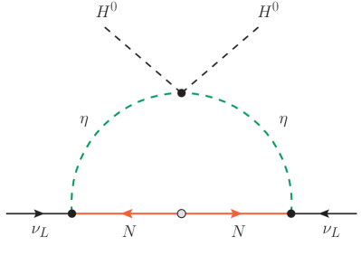
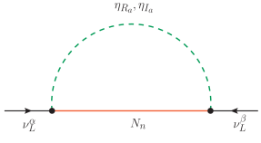
Figure 1: Neutrino mass generation. To the left, Feynman diagram with gauge eigenstates. To the right, the analogous Feynman diagram with the physical mass eigenstates that propagate in the loop.

The generation of neutrino masses takes place at the 1-loop level à la scotogenic [7]. In the presence of the terms given in Eqs. (1) and (2), lepton number is explicitly broken in two units, hence inducing Majorana neutrino masses. Assuming that the potential is such that the $\eta_{a}$ scalars do not get VEVs, see Eq. (3), neutrino masses are forbidden at tree-level. Nevertheless, they are induced at the 1-loop level, as shown in Fig. 1. Several diagrams contribute to the neutrino mass matrix. Therefore, one can write

$$\left(m_{\nu}\right)_{\alpha\beta}=\sum_{A,a,n}\left(m_{\nu}^{A}\right)_{\alpha\beta}^{an}\,,$$ (13)

where $\left(m_{\nu}^{A}\right)_{\alpha\beta}^{an}$ is the contribution to $\left(m_{\nu}\right)_{\alpha\beta}$ generated by the $N_{n}-\eta_{A_{a}}$ loop, given by

$$-i\left(m_{\nu}^{A}\right)_{\alpha\beta}^{an}=C^{A}_{na\alpha}\,\int\frac{\text{d}^{D}k}{\left(2\pi\right)^{D}}\frac{i}{k^{2}-m^{2}_{A_{a}}}\frac{i\left(\not{k}+M_{N_{n}}\right)}{k^{2}-M^{2}_{N_{n}}}\ C^{A}_{na\beta}\,,$$ (14)

where $D=4-\varepsilon$ is the number of space-time dimensions, the external neutrinos are taken at rest and $k$ is the momentum running in the loop. We note that the term proportional to $\not{k}$ does not contribute because it is odd in the loop momentum. $C^{A}_{na\alpha}$ is the $N_{n}-\eta_{A_{a}}-\nu_{L}^{\alpha}$ coupling, given by

$$C^{A}_{na\alpha}=i\,\frac{\kappa_{A}}{\sqrt{2}}\,\sum_{b}\,\left(V_{A}\right)^{*}_{ba}\,y_{nb\alpha}\,,$$ (15)

with $\kappa_{R}=1$ and $\kappa_{I}=i$. Since we assume real parameters in the scalar sector, complex conjugation in $V_{A}$ will be dropped in the following. Replacing Eq. (15) into Eq. (14) and introducing the standard Passarino-Veltman loop function $B_{0}$ [82],

$$B_{0}\left(0,m_{A_{a}}^{2},M_{N_{n}}^{2}\right)=\Delta_{\varepsilon}+1-\frac{m_{A_{a}}^{2}\log m_{A_{a}}^{2}-M_{N_{n}}^{2}\log M_{N_{n}}^{2}}{m_{A_{a}}^{2}-M_{N_{n}}^{2}},$$ (16)

where $\Delta_{\varepsilon}$ diverges in the limit $\varepsilon\to 0$, Eq. (13) becomes

$$\boxed{\left(m_{\nu}\right)_{\alpha\beta}=-\frac{1}{32\pi^{2}}\sum_{A,a,b,c,n}\,M_{N_{n}}\,\kappa_{A}^{2}\left(V_{A}\right)_{ba}\,\left(V_{A}\right)_{ca}\,y_{nb\alpha}\,y_{nc\beta}\,B_{0}(0,m_{A_{a}}^{2},M_{N_{n}})\,.}$$ (17)

Eq. (17) constitutes our central result for the 1-loop neutrino mass matrix in the model. It is important to note that the divergent pieces cancel exactly. Indeed, the $\kappa_{A}^{2}$ factor implies that the term proportional to $\Delta_{\varepsilon}$ in Eq. (17) involves the combination

$$\sum_{a}\left[\left(V_{R}\right)_{ba}\ \left(V_{R}\right)_{ca}-\left(V_{I}\right)_{ba}\ \left(V_{I}\right)_{ca}\right]=\left(V_{R}\,V_{R}^{T}\right)_{bc}-\left(V_{I}\,V_{I}^{T}\right)_{bc}=\delta_{bc}-\delta_{bc}=0\,,$$ (18)

which vanishes due to the orthogonality of the $V_{A}$ matrices, ensuring the cancellation of the divergent part of the $B_{0}$ functions. This was expected since the neutrino mass matrix is physical and therefore finite.

While Eq. (17) provides a simple analytical expression for the neutrino mass matrix, the dependence on the fundamental parameters of the model is not explicit. The neutrino mass matrix involves a product of $V_{A}$ matrices and $B_{0}$ functions, both in general depending on the scalar potential parameters in a non-trivial way. In order to identify more clearly the role of the scalar potential parameters, we will work under the assumptions in Eq. (9) and derive an approximate form for the neutrino mass matrix, valid for small $\lambda_{5}^{ab}$ couplings and small mixing angles in the scalar sector. First, it is convenient to make an expansion in powers of $\lambda_{5}^{ab}\ll 1$. One can write

$$\left(m_{\nu}\right)_{\alpha\beta}=-\frac{1}{32\pi^{2}} \sum_{n}\ M_{N_{n}}\ \sum_{a,b,c}\ y_{nb\alpha}\ y_{nc\beta}$$ (19)

$$\left\{\left[\left(V\right)_{ba}\ \left(V\right)_{ca}\right]^{(0)}\ \left[B_{0}^{(1)}(0,m_{R_{a}}^{2},M_{N_{n}})-B_{0}^{(1)}(0,m_{I_{a}}^{2},M_{N_{n}})\right]\right.$$

$$+\left.\left[\left(V_{R}\right)_{ba}\ \left(V_{R}\right)_{ca}-\left(V_{I}\right)_{ba}\ \left(V_{I}\right)_{ca}\right]^{(1)}\ B_{0}^{(0)}(0,m_{a}^{2},M_{N_{n}})\right\}+\mathcal{O}\left(\lambda_{5}^{2}\right)\,,$$

where the superindex ⁽ⁱ⁾, with $i=0,1$, denotes the order in $\lambda_{5}^{ab}$. We highlight that the expansion begins at 1st order in $\lambda_{5}$. This was indeed expected, since $\lambda_{5}=0$ would imply the restoration of lepton number and massless neutrinos. With this in mind, the origin of the two terms in Eq. (19) is easy to understand. In the first term, the $\lambda_{5}^{ab}$ couplings are neglected in the $V_{A}$ matrices but kept at leading order in the $B_{0}$ functions. This term is proportional to the $B_{0}(0,m_{R_{a}}^{2},M_{N_{n}})-B_{0}(0,m_{I_{a}}^{2},M_{N_{n}})$ difference, which would vanish for $\lambda_{5}^{aa}=0$, see Eqs. (10) and (11). The mass matrices for the real and imaginary components of $\eta^{0}$ are equal at 0th order in $\lambda_{5}$, $\widehat{\mathcal{M}}_{R}^{2\,(0)}=\widehat{\mathcal{M}}_{I}^{2\,(0)}$, and then we can define $V\equiv V_{R}^{(0)}=V_{I}^{(0)}$. In the second term, the $\lambda_{5}^{ab}$ couplings are neglected in the $B_{0}$ functions but kept at leading order in the $V_{A}$ mixing matrices. Since $m_{R_{a}}^{(0)}=m_{I_{a}}^{(0)}\equiv m_{a}$ at 0th order in $\lambda_{5}^{aa}$, then the $B_{0}^{(0)}$ function has the argument

$$m_{a}^{2}=\left(m_{\eta}^{2}\right)_{aa}+\left(\lambda_{3}^{aa}+\lambda_{4}^{aa}\right)\,\frac{v^{2}}{2}\,.$$ (20)

We note that this term will only be non-zero when the $\lambda_{5}$ matrix contains non-vanishing off-diagonal entries, since this is the only way the $\left(V_{R}\right)_{ba}\ \left(V_{R}\right)_{ca}-\left(V_{I}\right)_{ba}\ \left(V_{I}\right)_{ca}$ would not vanish at 1st order in $\lambda_{5}$. Next, we find approximate expressions for the $V_{A}$ mixing matrices. This is only feasible by assuming small scalar mixing angles, in agreement with Eq. (9). In this case one can expand $V$ not only in powers of $\lambda_{5}$, but also in powers of the small parameter

$$s_{ab}=\frac{1}{2}\,\left(\lambda_{3}^{ab}+\lambda_{4}^{ab}\right)\,\frac{v^{2}}{m_{b}^{2}-m_{a}^{2}}\ll 1\,,$$ (21)

which is defined for $a\neq b$ and corresponds to $\sin\theta_{R}^{ab}$ or $\sin\theta_{I}^{ab}$ at 0th order in $\lambda_{5}$, see Eq. (12). With this definition, one finds the general expression $\left(V\right)_{ab}=\delta_{ab}+(1-\delta_{ab})\,s_{ab}+\mathcal{O}\left(s^{2}\right)$. Analogous expressions are found for $V_{R}$ and $V_{I}$ replacing $s$ by $\sin\theta_{R}$ and $\sin\theta_{I}$, respectively. With all these ingredients, Eq. (19) can be written as

$$\boxed{\left(m_{\nu}\right)_{\alpha\beta}=\frac{v^{2}}{32\pi^{2}}\sum_{n,a,b}\frac{y_{na\alpha}\,y_{nb\beta}}{M_{N_{n}}}\,\Gamma_{abn}+\mathcal{O}\left(\lambda_{5}^{2}\right)+\mathcal{O}\left(\lambda_{5}\,s^{2}\right)\,,}$$ (22)

where we have defined the dimensionless quantity

$$\Gamma_{abn}=\delta_{ab}\,\lambda_{5}^{aa}\,f_{an}-(1-\delta_{ab})\left[\left(\lambda_{5}^{aa}\,f_{an}-\lambda_{5}^{bb}\,f_{bn}\right)\,s_{ab}-\frac{M^{2}_{N_{n}}}{m_{b}^{2}-m_{a}^{2}}\,\lambda_{5}^{ab}\ g_{abn}\right]$$ (23)

and the loop functions

$$f_{an} =\frac{M_{N_{n}}^{2}}{m_{a}^{2}-M_{N_{n}}^{2}}+\frac{M_{N_{n}}^{4}}{\left(m_{a}^{2}-M_{N_{n}}^{2}\right)^{2}}\log\frac{M_{N_{n}}^{2}}{m_{a}^{2}}\,,$$ (24)

$$g_{abn} =\frac{m_{a}^{2}}{m_{a}^{2}-M_{N_{n}}^{2}}\log\frac{M_{N_{n}}^{2}}{m_{a}^{2}}-\frac{m_{b}^{2}}{m_{b}^{2}-M_{N_{n}}^{2}}\log\frac{M_{N_{n}}^{2}}{m_{b}^{2}}\,.$$ (25)

Eq. (22) involves the quantity $\Gamma_{abn}$, which we have written in Eq. (23) as the sum of two terms. The first term in $\Gamma_{abn}$ contributes only for $a=b$ and involves only diagonal elements of $\lambda_{5}$. The second term, which involves diagonal as well as off-diagonal elements of $\lambda_{5}$, only contributes for $a\neq b$. We also note that $g_{abn}=-g_{ban}$.

Eq. (22) is the main analytical result of our work. Under the assumptions of Eq. (9), it reproduces the neutrino mass matrix in very good approximation. It is valid for any $n_{N}$ and $n_{\eta}$ values. We will now show how in some particular cases it reduces to well-known expressions in the literature.

3.1 Particular case 1: $\boldsymbol{(n_{N},n_{\eta})=(3,1)}$

The first example we consider is the standard Scotogenic model originally introduced in [7] and obtained for $(n_{N},n_{\eta})=(3,1)$. In this case, only one inert doublet $\eta$ is introduced. Therefore all the matrices in the scalar sector become just scalar parameters: $V_{A}=1$, $\lambda_{5}^{ab}\equiv\lambda_{5}^{11}\equiv\lambda_{5}$ and $(m_{\eta}^{2})_{aa}\equiv(m_{\eta}^{2})_{11}\equiv m_{\eta}^{2}$. Besides, the Yukawa couplings become $3\times 3$ matrices: $y_{na\alpha}\equiv y_{n1\alpha}\equiv y_{n\alpha}$. Similarly, $f_{an}\equiv f_{1n}\equiv f_{n}$, and the second term in Eq. (23) does not contribute. With these simplifications, the general $\Gamma_{abn}$ reduces to $\Gamma_{n}^{(3,1)}$, given by

$$\Gamma_{abn}^{(3,1)}\equiv\Gamma_{11n}^{(3,1)}\equiv\Gamma_{n}^{(3,1)}=\lambda_{5}\,f_{n}\,.$$ (26)

Replacing this into Eq. (22), one obtains the well-known neutrino mass matrix

$$\left(m_{\nu}\right)_{\alpha\beta}^{(3,1)}=\frac{\lambda_{5}\,v^{2}}{32\pi^{2}}\sum_{n}\frac{y_{n\alpha}\,y_{n\beta}}{M_{N_{n}}}\left[\frac{M_{N_{n}}^{2}}{m_{0}^{2}-M_{N_{n}}^{2}}+\frac{M_{N_{n}}^{4}}{\left(m_{0}^{2}-M_{N_{n}}^{2}\right)^{2}}\log\frac{M_{N_{n}}^{2}}{m_{0}^{2}}\right]\,,$$ (27)

with $m_{0}^{2}=m_{\eta}^{2}+(\lambda_{3}+\lambda_{4})\,v^{2}/2$. This expression agrees with [7] up to a factor of $1/2$ that was missing in the original reference. 

3.2 Particular case 2: $\boldsymbol{(n_{N},n_{\eta})=(1,2)}$

A version of the Scotogenic model with one singlet fermion and two inert doublets, $(n_{N},n_{\eta})=(1,2)$, has been considered in [79, 80]. Since the model contains only one singlet fermion $N$, $M_{N_{n}}\equiv M_{N}$ is just a parameter. The Yukawa couplings become $2\times 3$ matrices: $y_{na\alpha}\equiv y_{1a\alpha}\equiv y_{a\alpha}$. Finally, $f_{na}\equiv f_{1a}\equiv f_{a}$ and $g_{abn}\equiv g_{ab1}\equiv g_{ab}$. Both references work in the basis in which the $m_{\eta}^{2}$ matrix is diagonal. However, they take different simplifying assumptions about the scalar potential parameters.

In [79] the matrix $\lambda_{3}+\lambda_{4}$ was assumed to be diagonal. In this case, which we denote as scenario $(1,2)_{\rm\,I}$, $(1-\delta_{ab})s_{ab}=0$ and the general $\Gamma_{abn}$ reduces to

$$\Gamma_{abn}^{(1,2)_{\rm\,I}}\equiv\Gamma_{ab1}^{(1,2)_{\rm\,I}}\equiv\Gamma_{ab}^{(1,2)_{\rm\,I}}=\delta_{ab}\,\lambda_{5}^{aa}\,f_{an}+(1-\delta_{ab})\,\frac{M^{2}_{N_{n}}}{m_{b}^{2}-m_{a}^{2}}\,\lambda_{5}^{ab}\ g_{abn}\,.$$ (28)

Replacing this expression into Eq. (22) and arranging the different pieces properly, one obtains

$$\left(m_{\nu}\right)_{\alpha\beta}^{(1,2)_{\rm\,I}}=\frac{v^{2}}{32\pi^{2}}\sum_{a,b}y_{a\alpha}\,y_{b\beta}\,\lambda_{5}^{ab}\,\frac{M_{N}}{m_{b}^{2}-M_{N}^{2}}\left[\frac{m_{b}^{2}}{m_{a}^{2}-m_{b}^{2}}\log\frac{m_{a}^{2}}{m_{b}^{2}}-\frac{M_{N}^{2}}{m_{a}^{2}-M_{N}^{2}}\log\frac{m_{a}^{2}}{M_{N}^{2}}\right]\,,$$ (29)

which agrees with the result in [79] up to a global factor of $1/4$.

On the other hand, a diagonal $\lambda_{5}$ matrix was taken in [80]. We denote this as scenario $(1,2)_{\rm\,II}$. Again, this simplifies $\Gamma_{abn}$, which becomes

$$\Gamma_{abn}^{(1,2)_{\rm\,II}}\equiv\Gamma_{ab1}^{(1,2)_{\rm\,II}}\equiv\Gamma_{ab}^{(1,2)_{\rm\,II}}=\delta_{ab}\,\lambda_{5}^{aa}\,f_{an}-(1-\delta_{ab})\left(\lambda_{5}^{aa}\,f_{an}-\lambda_{5}^{bb}\,f_{bn}\right)\,s_{ab}\,.$$ (30)

With this result, one can easily use Eq. (22) to derive

$$\left(m_{\nu}\right)_{\alpha\beta}^{(1,2)_{\rm\,II}}=\frac{v^{2}}{32\pi^{2}M_{N}}\,\sum_{a,b,c}\,y_{a\alpha}\,y_{b\beta}\,\lambda_{5}^{cc}\,f_{c}\,X_{abc}\,,$$ (31)

with

$$X_{abc}=\delta_{ab}\delta_{bc}+\frac{1}{2}\,(1-\delta_{ab})\left(\delta_{c2}-\delta_{c1}\right)\,\left(\lambda_{3}^{ab}+\lambda_{4}^{ab}\right)\,\frac{v^{2}}{m_{b}^{2}-m_{a}^{2}}\,,$$ (32)

which agrees with the expression given in [80] if terms of order $s_{12}^{2}$ are neglected.

4 High-energy behavior

The conservation of the $\mathbb{Z}_{2}$ parity is crucial for the Scotogenic setup to be consistent. In the absence of this symmetry, neutrinos would acquire masses at tree-level and the DM candidate would no longer be stable. This motivates the study of the conservation of $\mathbb{Z}_{2}$ at high energies, a line of work initiated in [83]. As pointed out in this reference, the RGE flow in the Scotogenic model might alter the shape of the scalar potential at high energies and lead to the breaking of $\mathbb{Z}_{2}$. This issue was fully explored in subsequent works [85, 86], which show that the breaking of the $\mathbb{Z}_{2}$ parity actually takes place in large regions of the parameter space. A similar discussion for a variation of the Scotogenic model including scalar and fermion triplets was presented in [48].

Some general features of the high-energy behavior of the model, and in particular of the possible breaking of the $\mathbb{Z}_{2}$ symmetry, can be understood by inspecting the 1-loop $\beta$ function for the $m_{\eta}^{2}$ parameter, shown in Appendix A. Eq. (39) generalizes the result previously derived in [83] and gives the 1-loop $\beta$ function for the $m_{\eta}^{2}$ matrix, valid for any values of $(n_{N},n_{\eta})$. In order to study the possible breaking of $\mathbb{Z}_{2}$, one must consider the sign (positive or negative) of the individual contributions to the running of $m_{\eta}^{2}$. In this regard, the negative contribution of the term proportional to $\text{Tr}\left[y_{a}^{\dagger}M_{N}^{\ast}M_{N}y_{b}\right]$ turns out to be crucial. In the following, we will refer to this term as the trace term. As first pointed out in [83] for the standard Scotogenic model, in case of large Yukawa couplings (equivalent to $\lambda_{5}\ll 1$) and $M_{N}^{2}\gtrsim m_{\eta}^{2}$, the trace term dominates the $m_{\eta}^{2}$ running and drives it towards negative values. Eventually, this leads to the breaking of the $\mathbb{Z}_{2}$ symmetry at high energies, once $m_{\eta}^{2}<0$ induces a minimum of the scalar potential with $\langle\eta\rangle\neq 0$. The same behavior is expected in the general Scotogenic model. Other terms in Eq. (39) may counteract this effect. In particular, the terms proportional to the quartic scalar couplings may do so if their signs are properly chosen. The contribution to the $m_{\eta}^{2}$ running will be positive for $\lambda_{2}>0$ and $\lambda_{3,4}<0$ (since $m_{H}^{2}<0$), while their effect will reinforce that of the trace term otherwise.

We will now explore the scalar potential of the model at high energies by solving the full set of RGEs numerically. In order to do that we will concentrate on two specific (but representative) versions of the general Scotogenic model:

• The $\boldsymbol{(3,1)}$ model, with three singlet fermions and one inert doublet. This is the original Scotogenic model [7].

• The $\boldsymbol{(1,3)}$ model, with one singlet fermion and three inert doublets.

We set all model parameters at the electroweak scale, which we take to be the $Z$-boson mass, $m_{Z}$. Therefore, in the following all values for the input parameters must be understood to hold at $\mu=m_{Z}$. We compute $m_{H}^{2}$ by solving the tadpole equations of the model and set the $\lambda_{1}$ value to reproduce the measured Higgs boson mass. The remaining scalar potential parameters are chosen freely, but always to values that guarantee that the potential is bounded from below (BFB) at the electroweak scale. This is a non-trivial requirement due to the complexity of the scalar potential of the general Scotogenic model. We refer to Appendix B for a detailed discussion on how we check boundedness from below. Finally, we must accommodate the neutrino squared mass differences and the leptonic mixing angles measured in neutrino oscillation experiments by properly fixing the Yukawa couplings of the model. In the two variants of the general Scotogenic model considered the Yukawa couplings become $3\times 3$ matrices, and then they can be obtained by means of a Casas-Ibarra parametrization [87], adapted to the Scotogenic model as explained in [88, 89, 90, 91]. This allows us to write the Yukawa matrices in full generality as

$$y=i\,V^{\dagger}\,\Sigma^{-1/2}\,R\,D_{\sqrt{m}}\,U^{\dagger}\,.$$ (33)

Here $U$ is a $3\times 3$ unitary matrix, defined by the Takagi decomposition of the neutrino mass matrix

$$U^{T}\,m_{\nu}\,U=\text{diag}\left(m_{1},m_{2},m_{3}\right)\,,$$ (34)

with $m_{i}$ the three physical neutrino masses. $R$ is a general $3\times 3$ orthogonal matrix and we have defined $D_{\sqrt{m}}=\text{diag}\left(\sqrt{m_{1}},\sqrt{m_{2}},\sqrt{m_{3}}\right)$. Finally, $\Sigma$ and $V$ are determined by the matrix $M$, defined implicitly by the general expression $m_{\nu}=y^{T}\,M\,y$. $\Sigma=\text{diag}\left(\sigma_{1},\sigma_{2},\sigma_{3}\right)$ is a diagonal matrix containing the eigenvalues of $M$, while $V$ is a $3\times 3$ unitary matrix such that $M=V^{T}\,\Sigma\,V$. Indeed, as shown in Sec. 3, the analytical expression for the neutrino mass matrix in Eq. (22) can be particularized to the $(3,1)$ and $(1,3)$ models and in both cases one can write $m_{\nu}$ as the matrix product $y^{T}\,M\,y$, with different forms for the matrix $M$. With these definitions, Eq. (33) ensures compatibility with neutrino oscillation data. We consider neutrino normal mass ordering and the $1\,\sigma$ ranges for the oscillation parameters obtained in the global fit [92], including the CP-violating phase $\delta$, hence allowing for complex Yukawa couplings. For simplicity, we take $m_{1}=0$ and $R=\mathbb{I}$, with $\mathbb{I}$ the $3\times 3$ identity matrix. 

Some comments are in order before presenting our numerical results. In what follows, several regions of the parameter spaces of the $(3,1)$ and $(1,3)$ Scotogenic models will be explored. Our focus is the study of the behavior of these models at high energies. While several phenomenological directions of interest can be pursued, these are beyond the scope of our work. In particular, we are interested in effects associated to the trace term, what motivates the consideration of small $\lambda_{5}$ values ($\lambda_{5}^{aa}\leq 10^{-8}$). Larger $\lambda_{5}$ entries would require smaller $y$ Yukawa couplings in order to accommodate the mass scales measured in neutrino oscillations experiments, see Eqs. (27), (29) and (31), hence making the trace term numerically less relevant. For this reason, all scenarios considered below have $y\sim\mathcal{O}(1)$. While this may lead to conflict with the current bounds from the non-observation of charged lepton flavor violating processes, we note the existence of many free parameters in the $y$ Yukawa matrices. This freedom can be used to cancel the most constraining observables, for instance by choosing specific $R$ matrices, without any impact on our discussion. Similarly, the scenarios considered below, and in particular the values chosen for the masses of the $\mathbb{Z}_{2}$-odd states, may not be compatible with the measured dark matter relic density.

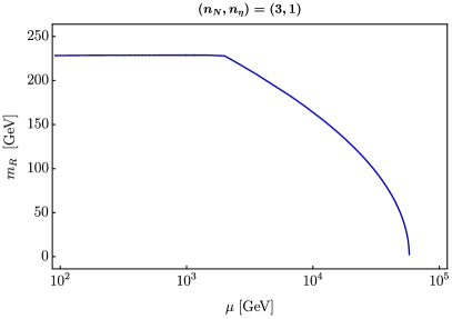
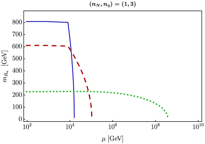
Figure 2: Evolution of the CP-even scalar masses as a function of the energy scale $\mu$ in the $(3,1)$ and $(1,3)$ Scotogenic models. To the left, the CP-even scalar mass $m_{R}$ in the standard $(3,1)$ model with $M_{N}=(1,1.5,2)$ TeV, $\lambda_{2}=\lambda_{3}=\lambda_{4}=0.1$, $\lambda_{5}=10^{-9}$ and $m_{\eta}^{2}=(200$ GeV$)^{2}$. To the right, the three CP-even scalar masses $m_{R_{a}}$ in the $(1,3)$ model with $M_{N}=8$ TeV, $\lambda_{2}^{aaaa}=\lambda_{3}^{aa}=\lambda_{4}^{aa}=0.1$, $\lambda_{5}^{aa}=10^{-9}$ and $m_{\eta}^{2}=(200^{2},600^{2},800^{2})$ GeV², with the remaining scalar parameters set to zero.

First, we have rediscovered the parity problem in the standard $(3,1)$ Scotogenic model. This is shown on the left-hand side of Fig. 2, which displays the RGE evolution of the CP-even scalar mass $m_{R}$ with the energy scale $\mu$. This is the most convenient parameter to study the breaking of the $\mathbb{Z}_{2}$ symmetry. When $m_{R}^{2}$ becomes negative, the lightest CP-even scalar becomes tachyonic, a clear sign that $\langle\eta\rangle=0$ is not the minimum of the potential. We have checked that the scalar potential is BFB at all energy scales in this figure. We note that due to our parameter choices the lightest singlet fermion, $N_{1}$, has vanishing Yukawa couplings. For the same reason, $y_{2\alpha}\ll y_{3\alpha}$ and the effect is driven predominantly by $N_{3}$. This explains the drastic change in the evolution of $m_{R}$ at $\mu=2$ TeV, when $N_{3}$ becomes active. Below this scale, $N_{3}$ effectively decouples and does not contribute to the RGE running. We point out that a much less pronounced change takes also place at $\mu=1.5$ TeV, when $N_{2}$ becomes active, but this is not visible on the figure. The $\mathbb{Z}_{2}$ parity gets broken at $\mu\simeq 60$ TeV, after which the $\eta_{R}$ state becomes tachyonic. These results agree well with those found in [83] and confirm the possible breaking of $\mathbb{Z}_{2}$ in the original Scotogenic model. A very similar behavior is found for the $(1,3)$ model, which only has one singlet fermion, as shown on the right-hand side of Fig. 2. In this case, the three CP-even scalar masses $m_{R_{a}}$ are displayed. Again, we have checked that the scalar potential is BFB at all energy scales in this figure. As in the case of the standard Scotogenic model, when one of the CP-even scalar masses reaches zero the $\mathbb{Z}_{2}$ symmetry gets broken. We see in this figure that this happens at $\mu\simeq 15$ TeV, where one of the scalar masses (the one receiving the largest contribution from the trace term) goes very sharply towards zero due to the effect of the large $M_{N}=8$ TeV value. This is clearly the same behavior observed in the standard $(3,1)$ Scotogenic model.

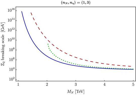
Figure 3: $\mathbb{Z}_{2}$ breaking scale as a function of the singlet fermion mass $M_{N}$ in the $(1,3)$ Scotogenic model for three different scenarios: $\lambda_{2}^{aaaa}=\lambda_{3}^{aa}=\lambda_{4}^{aa}=0.1$ and $m_{\eta}^{2}=\left(200^{2},300^{2},400^{2}\right)$ GeV² (blue), $\lambda_{2}^{aaaa}=\lambda_{3}^{aa}=\lambda_{4}^{aa}=0.1$ and $m_{\eta}^{2}=\left(200^{2},600^{2},800^{2}\right)$ GeV² (red, dashed), and $\lambda_{2}^{aaaa}=\lambda_{2}^{aabb}=\lambda_{3}^{aa}=\lambda_{4}^{aa}=0.3$ and $m_{\eta}^{2}=\left(200^{2},300^{2},400^{2}\right)$ GeV² (green, dotted). In the three cases $\lambda_{5}^{aa}=10^{-9}$ and the remaining quartic parameters are set to zero.

In the following we concentrate on the $(1,3)$ model. As already discussed, the singlet fermion mass $M_{N}$ drives the scalar masses towards negative values via the trace term, hence breaking the $\mathbb{Z}_{2}$ parity at high energies. Fig. 3 shows the $\mathbb{Z}_{2}$ breaking scale as a function of $M_{N}$ for several scalar parameter sets. The blue and red lines correspond to moderate values for the quartic couplings, $\lambda_{2}^{aaaa}=\lambda_{3}^{aa}=\lambda_{4}^{aa}=0.1$, while the green line has increased (and additional) quartics, $\lambda_{2}^{aaaa}=\lambda_{2}^{aabb}=\lambda_{3}^{aa}=\lambda_{4}^{aa}=0.3$. The $\lambda_{5}$ matrix is taken to be diagonal, with $\lambda_{5}^{aa}=10^{-9}$. We have explicitly checked that the scalar potential is BFB at the electroweak scale in all scenarios.  As expected, the $\mathbb{Z}_{2}$ breaking scale decreases for larger $M_{N}$ since the effect of the trace term becomes stronger. While different scalar potential couplings may alter the outcome, this generic behavior is found in large portions of the parameter space. One should notice, however, that the green curve begins at $M_{N}\simeq 2$ TeV. For this specific scenario, lower values of $M_{N}$ do not break the $\mathbb{Z}_{2}$ symmetry, as we now proceed to discuss.

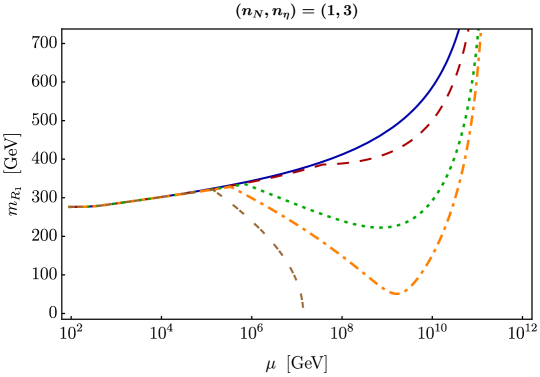
Figure 4: Evolution of the lightest scalar mass $m_{R_{1}}$ as a function of the energy scale $\mu$ in the $(1,3)$ Scotogenic model. The scalar parameters are set to $\lambda_{2}^{aaaa}=\lambda_{2}^{aabb}=\lambda_{3}^{aa}=\lambda_{4}^{aa}=0.3$, $\lambda_{5}^{aa}=10^{-9}$ and $m_{\eta}^{2}=\left(200^{2},300^{2},400^{2}\right)$ GeV², while $M_{N}$ takes the values $1$ TeV (blue), $1.5$ TeV (red, dashed), $1.9$ TeV (green, dotted), $2.025$ TeV (orange, dash-dotted) and $2.2$ TeV (brown, double dashed).

Fig. 4 shows the evolution of the lightest scalar mass $m_{R_{1}}$ as a function of the energy for the parameter values corresponding to the green curve in Fig. 3. The results have been obtained for several values of $M_{N}$. It is important to note that this figure shows the mass of the lightest scalar at each energy scale, and not the mass of a single mass eigenstate at all energies. For $M_{N}=2.2$ TeV one observes that $m_{R_{1}}$ reaches zero and the $\mathbb{Z}_{2}$ symmetry gets broken at $\mu\simeq 10^{7}$ GeV, in accordance with Fig. 3. For lower $M_{N}$ values, however, $m_{R_{1}}$ never reaches zero. Although $m_{R_{1}}$ gets initially decreased due to the effect of the trace term, it eventually increases at higher energies. The reason is the appearance of a Landau pole in the $\lambda_{2}$ quartic couplings. In this figure $\lambda_{2}^{aaaa}=\lambda_{2}^{aabb}=0.3$ at the electroweak scale, and this value grows with the energy until it completely dominates the $m_{\eta}^{2}$ $\beta$ function with a positive contribution, see Eq. (39). The high multiplicity of $\lambda_{2}$ couplings reinforces the effect. Actually, we note that this Landau pole is present at very high energies, well above the $\mathbb{Z}_{2}$ breaking scale, for many choices of the parameters at the electroweak scale.

Figure 5: $\mathbb{Z}_{2}$ breaking scale as a function of the $\lambda_{2}^{2233}$ parameter in the $(1,3)$ Scotogenic model for three different scenarios: $\lambda_{2}^{aaaa}=\lambda_{3}^{aa}=\lambda_{4}^{aa}=0.1$, $\lambda_{5}^{aa}=10^{-8}$, $m_{\eta}^{2}=\left(200^{2},300^{2},400^{2}\right)$ GeV² and $M_{N}=5$ TeV (blue), $\lambda_{2}^{aaaa}=\lambda_{3}^{aa}=\lambda_{4}^{aa}=0.1$, $\lambda_{5}^{aa}=10^{-9}$, $m_{\eta}^{2}=\left(200^{2},250^{2},300^{2}\right)$ GeV² and $M_{N}=1.25$ TeV (red, dashed), and $\lambda_{2}^{aaaa}=\lambda_{2}^{aabb}=\lambda_{3}^{aa}=\lambda_{4}^{aa}=0.3$, $\lambda_{5}^{aa}=10^{-8}$, $m_{\eta}^{2}=\left(200^{2},600^{2},800^{2}\right)$ GeV² and $M_{N}=9$ TeV (green, dotted). In the three cases the remaining quartic parameters are set to zero.

We conclude our exploration of the high-energy behavior of the $(1,3)$ model with Fig. 5. In this case we plot the $\mathbb{Z}_{2}$ breaking scale as a function of one of the $\lambda_{2}$ parameters, namely $\lambda_{2}^{2233}$. This is done for three scenarios: the blue curve corresponds to $\lambda_{2}^{aaaa}=\lambda_{3}^{aa}=\lambda_{4}^{aa}=0.1$, $\lambda_{5}^{aa}=10^{-8}$, $m_{\eta}^{2}=\left(200^{2},300^{2},400^{2}\right)$ GeV² and $M_{N}=5$ TeV, in red we show the results for $\lambda_{2}^{aaaa}=\lambda_{3}^{aa}=\lambda_{4}^{aa}=0.1$, $\lambda_{5}^{aa}=10^{-9}$, $m_{\eta}^{2}=\left(200^{2},250^{2},300^{2}\right)$ GeV² and $M_{N}=1.25$ TeV, while the green line is for $\lambda_{2}^{aaaa}=\lambda_{2}^{aabb}=\lambda_{3}^{aa}=\lambda_{4}^{aa}=0.3$, $\lambda_{5}^{aa}=10^{-8}$, $m_{\eta}^{2}=\left(200^{2},600^{2},800^{2}\right)$ GeV² and $M_{N}=9$ TeV. In all cases we have checked that the scalar potential is BFB at the electroweak scale. For the blue and green lines, the impact of $\lambda_{2}^{2233}$ is relatively mild. This is because the high values of $M_{N}$ ($5$ and $9$ TeV, respectively) make the trace term completely dominant and break the $\mathbb{Z}_{2}$ symmetry at relatively low energies. In contrast, the $\mathbb{Z}_{2}$ breaking scale has a much stronger dependence on $\lambda_{2}^{2233}$ in the red scenario, which has a lower $M_{N}=1.25$ TeV. For $\lambda_{2}^{2233}\gtrsim 0.6$, a Landau pole is found before the $\mathbb{Z}_{2}$ symmetry gets broken.

5 Thermal effects and the fate of the $\boldsymbol{\mathbb{Z}_{2}}$ symmetry

To determine the cosmological impact of $\mathbb{Z}_{2}$ breaking one needs to take into account thermal corrections. This is because the interaction with the hot, primordial plasma induces an effective potential for the scalar fields. This effective potential, at 1-loop order, is given by

$$V_{\rm 1-loop}(\eta,T)=V_{\rm CW}(\eta)+\frac{T^{4}}{2\pi}\left[n_{B}J_{B}(m^{2}(\eta)/T^{2})-n_{f}J_{F}(m_{f}(\eta)^{2}/T^{2})\right]\,.$$ (35)

Here $V_{\rm CW}$ is the standard Coleman-Weinberg potential for $\eta$ at zero temperature while $J_{B}(m_{b}(\eta)^{2}/T^{2})$ and $J_{F}(m_{f}(\eta)^{2}/T^{2})$ are the bosonic and fermionic functions, respectively. These functions admit a high-T expansion (see [93] for a review) which allows to write the scalar mass as

$$m_{\eta}^{2}(T)\sim m_{\eta}^{2}+c\,T^{2}\,.$$ (36)

The coefficient $c$ depends on the details of the theory, such as the quartic, gauge and Yukawa couplings.  At any given time in the early Universe, as it can be seen in Eq. (36), the effect of the temperature is usually to restore the symmetry with the subsequent dilution of the effects of the running that we have discussed in the previous section. It is therefore mandatory to study if temperature has any impact on the fate of the $\mathbb{Z}_{2}$ symmetry and, therefore, on the stability of DM.

During inflation, the $\eta$ field is expected to have large quantum fluctuations, comparable to the Hubble parameter in this period, $H_{I}$. These fluctuations can be much larger than the scalar mass at zero temperature and, acting as a sort of random walk, might bring the field to a vacuum where the $\mathbb{Z}_{2}$ is broken. Right after reheating, when the temperature is potentially very large, the thermal mass of the scalar field may be large enough to overcome all breaking effects. The reason is that, assuming the decay of the inflaton is fast enough (instantaneous reheating, $\Gamma_{\Phi}\sim H_{I}$), the reheating temperature is roughly given by [96]

$$T_{\rm RH}\sim 10^{-1}\,\sqrt{H_{I}\,M_{P}}\,,$$ (37)

where $M_{P}$ is the Planck mass. Note that this temperature is generically much larger than $H_{I}$. If the number of e-folds is not exceedingly large, $T_{\rm RH}$ is expected to be larger than any field excursion and we expect $m_{\eta}(T_{\rm RH})^{2}>0$. In addition, this also implies that $m_{\eta}(T_{\rm RH})^{2}\sim c\,T_{\rm RH}^{2}\gg H(T_{\rm RH})^{2}$, meaning that the field will fastly roll down to the minimum, at zero value $\left\langle\eta\right\rangle=0$. 

As the temperature decreases, it may happen that RGE effects make the $\mathbb{Z}_{2}$ breaking to occur at some high-energy scale. However, the $\eta$ field will be already at $\left\langle\eta\right\rangle=0$, meaning that it cannot experience such a breaking. As the temperature continues decreasing, we reach the freeze-out temperature. From this point on, any breaking of the dark parity would be a disaster for the DM stability. Note however, that since the $\eta$ field is at its local minimum, $\left\langle\eta\right\rangle=0$, it cannot notice this high-energy RGE induced symmetry breaking as it will only feel the local properties of the vacuum around $\left\langle\eta\right\rangle=0$.

Of course, this does not mean that RGE effects are completely harmless for the Scotogenic model. In fact, the RGE-induced breaking could induce the appearance of deeper minima in the potential, implying that the stability of DM is just a local property of our vacuum, which could be a false vacuum, and not a global feature of the potential.

6 Summary and discussion

The Scotogenic model is a well-known radiative scenario for the generation of neutrino masses. The introduction of three singlet fermions and one inert scalar doublet, all charged under a new $\mathbb{Z}_{2}$ parity, leads to 1-loop Majorana neutrino masses and, as a bonus, provides a viable weakly-interacting dark matter candidate. In this work we have considered a generalization of this setup to any numbers of generations of singlet fermions and inert doublets. After computing the 1-loop neutrino mass matrix in the general version of the model, we have studied its high-energy behavior, focusing on two specific variants: the original Scotogenic model with $(n_{N},n_{\eta})=(3,1)$ and a new multi-scalar variant with $(n_{N},n_{\eta})=(1,3)$. Our main conclusion is that all the features of the original model are kept in the multi-scalar version, with some particularities due to the presence of a more involved scalar sector.

Our generalization of the Scotogenic model offer several novel possibilities. For instance, flavor model building could benefit from an interesting feature of multi-scalar versions of the model. In the $(n_{N},n_{\eta})=(1,3)$ model, one obtains three massive neutrinos and leptonic mixing can be fully explained even if the Yukawa matrices are completely diagonal. In this case the leptonic mixing matrix would be generated by mixing in the scalar sector. This could be relevant in some flavor models. For example, it may be a crucial ingredient to rescue models where lepton mixing is predicted to be similar to quark mixing. Novel phenomenological signatures might exist as well. The $\eta$ doublets can be produced at the Large Hadron Collider due to their couplings to the SM gauge bosons. Exotic signatures might be possible in models with many $\eta$ generations, such as the $(n_{N},n_{\eta})=(1,3)$ model. Cascade decays initiated by the production of the heaviest $\eta$ doublets would lead to striking multilepton signatures, including missing energy due to the production of the lightest $\mathbb{Z}_{2}$-odd state at the end of the decay chain. Finally, the dark matter production rates in the early Universe might be affected as well by the presence of additional scalar degrees of freedom. These interesting questions certainly deserve further study.

Appendix A Renormalization Group Equations

At the 1-loop order, the RGEs of a model can be written as

$$\frac{dx(t)}{dt}=\frac{1}{16\pi^{2}}\,\beta_{x}\,,$$ (38)

where $t\equiv\log\mu$, $\mu$ is the renormalization scale and $\beta_{x}$ is the 1-loop $\beta$ function for the parameter $x$. In our analysis, the full 1-loop running in the Scotogenic model with arbitrary numbers of $N$ and $\eta$ generations has been considered. Analytical expressions for all the 1-loop $\beta$ functions have been derived with the help of SARAH [97, 98, 99, 100, 101].  These have been included in a code that solves the complete set of RGEs numerically.

We are mainly interested in the possible breaking of the $\mathbb{Z}_{2}$ parity at high energies, and this is associated to the running of the $m^{2}_{\eta}$ matrix. The corresponding 1-loop $\beta$ functions are given by

$$\begin{split}\left(\beta_{m^{2}_{\eta}}\right)_{ab}=&-\frac{9}{10}\,g_{1}^{2}\,\left(m^{2}_{\eta}\right)_{ab}-\frac{9}{2}\,g_{2}^{2}\,\left(m^{2}_{\eta}\right)_{ab}+\sum_{c,d=1}^{n_{\eta}}\left[4\,\lambda_{2}^{abcd}\left(m^{2}_{\eta}\right)_{dc}+2\,\lambda_{2}^{acdb}\left(m^{2}_{\eta}\right)_{cd}\right]\\ &+\left[4\,\lambda_{3}^{ab}+2\,\lambda_{4}^{ab}\right]\,m^{2}_{H}+\left(m^{2}_{\eta}\right)_{ab}\sum_{n=1}^{n_{N}}\sum_{\alpha=1}^{3}\left(\left|y_{na\alpha}\right|^{2}+\left|y_{nb\alpha}\right|^{2}\right)-4\,\text{Tr}\left[y_{a}^{\dagger}M_{N}^{\ast}M_{N}y_{b}\right]\,.\end{split}$$ (39)

Here $y_{a}\equiv\left[y_{na\alpha}\right]$ is a $n_{N}\times 3$ matrix, being the first index a singlet fermion family index and the third one a charged lepton family index. We have explicitly checked that for $n_{N}=3$ and $n_{\eta}=1$, Eq. (39) reduces to the $m^{2}_{\eta}$ $\beta$ function in the standard Scotogenic model [83].

Appendix B Boundedness from below

In order to ensure the existence of a stable vacuum, the scalar potential of the theory must be BFB. There exist several approaches to analyze boundedness from below. Ideally, one would like to have a BFB test that provides necessary and sufficient conditions. This way, one could not only guarantee that all potentials that pass the test are BFB (sufficient condition), but also discard potentials that fail it (necessary condition). In this regard, a major step forward was given in [102] and more recently in [103]. The algorithm proposed in the second reference provides necessary and sufficient conditions for boundedness from below in a generic scalar potential using notions of spectral theory of tensors. However, applying this algorithm beyond a few simple cases turns out to be impractical due to the computational cost involved. For this reason, in phenomenological analyses one usually resorts to less ambitious approaches which only provide sufficient conditions, but not necessary. These methods are overconstraining, since one must reject potentials not passing the test, even though they might actually be BFB. Nevertheless, if the potential passes the test, one can fully trust that boundedness from below is guaranteed.

Here we will employ the copositivity criterion, which combined with a recently developed mathematical algorithm, never applied to a high-energy physics scenario, will give us sufficient (but not necessary) conditions. To the best of our knowledge, the first paper relating copositivity with boundedness from below was [104]. One must first express the quartic part of the scalar potential, $\mathcal{V}_{4}$, as a quadratic form of the $n$ real fields $\varphi_{a}$ ($a=1,2,\dots n$) in the theory,

$$\mathcal{V}_{4}=\Lambda_{ab}\,\varphi_{a}^{2}\varphi_{b}^{2}\,.$$ (40)

The scalar potential is BFB if and only if the matrix of quartic couplings $\Lambda_{ab}$ is copositive. A real matrix $A$ is said to be copositive if $x^{T}A\,x\geqslant 0$ for every non-negative vector $x\geqslant 0$, that is, $x^{i}\geqslant 0$. If the inequality is strict, the matrix is strictly copositive. Therefore, checking for the copositivity of the matrix of quartic couplings would in principle provide sufficient and necessary boundedness from below conditions. However, in complicated models such as the general Scotogenic model, one cannot write $\mathcal{V}_{4}$ as a quadratic form without introducing mixed bilinears (scalar field combinations involving two different fields). For this reason, this method only leads to sufficient conditions, as we now explain.

In order to write the quartic part of the scalar potential as a quadratic form we define

$$\varphi_{i}^{\dagger}\varphi_{i}=h_{i}^{2}\,,\qquad\varphi_{i}^{\dagger}\varphi_{j}=\left|h_{i}\right|\left|h_{j}\right|\rho_{ij}e^{i\phi_{ij}}=h_{ij}^{2}\,\rho_{ij}e^{i\phi_{ij}}\,\,,$$ (41)

with $\left|\rho_{ij}\right|\in[0,1]$ by virtue of the Cauchy-Schwarz inequality. Thus, we can express the boundedness from below condition as

$$\mathcal{V}_{4}=x^{T}\,V_{4}\,x\geqslant 0\,,$$ (42)

with $x=\left(h_{1}^{2}\ \dots\ h_{i}^{2}\ \dots\ h_{ij}^{2}\ \dots\right)$ and the matrix $V_{4}$ is given by a combination of the quartic couplings, the $\lambda$’s, as well as the $\rho$’s and $\phi$ phases.  The reason why this method provides only sufficient conditions is the presence of the mixed bilinears. Notice that the direction given by $h_{ij}^{2}$ is not independent of $h_{i}^{2}$ and $h_{j}^{2}$. Therefore, imposing $x^{T}\,V_{4}\,x\geqslant 0$ for every non-negative $x$ vector is overconstraining, since unphysical directions would be included in the test. Nonetheless, when the test is positive, the potential is BFB. In summary, a scalar potential is BFB if the associated $V_{4}$ matrix is copositive. However, when the matrix is not copositive nothing can be said about the potential.

There is mathematical work showing that a symmetric matrix $A$ of order $n$ is (strictly) copositive if and only if every principal submatrix $B$ of $A$ has no eigenvector $w>0$ with associated eigenvalue $\kappa<0\ (\leqslant 0)$ [105]. However, these theorems are of little practical value when the matrix has a large order, since there will be $2^{n}-1$ principal submatrices. Luckily, we can make use of [106] instead. The authors of this work proposed an algorithm that leads to necessary and sufficient conditions for the copositivity of unit diagonal matrices (matrices with all diagonal elements equal to $1$). Although the algorithm in [106] could only be applied for up to $7\times 7$ matrices, incidentally the case in the $(1,3)$ Scotogenic model, more recent work by the same authors contains indications to extend it to higher orders [107].

After all these considerations, our procedure to check for copositivity is as follows:

1. We replace all the quartic couplings in $V_{4}$ by the numerical values in the scalar potential we want to test.

2. We transform each element of the matrix to the worst case scenario. This is achieved by treating the remaining $\rho$ and $\phi$ parameters as independent variables and setting them to the configuration for which the term is minimal. 

3. We check if the matrix has null entries in the diagonal. If it does, we remove the corresponding rows and columns. The original matrix will be copositive if the remaining one is and the removed elements are non-negative.

4. We need the matrix to have unit diagonal to be able to apply the algorithm in [106]. Therefore, we divide all its entries by the smallest element in the diagonal and we replace all the values greater than $1$ by $1$. The original matrix will be copositive if the new one is.

5. We finally check the copositivity of the resulting matrix with the algorithm in [106].

A final remark about our method is in order. The stability in charge-breaking directions is ignored in many analyses. However, since we are being overly restrictive treating all the $\rho$ moduli and $\phi$ phases as independent variables in the different entries of $V_{4}$, charge-breaking directions are included as well in our BFB test. In order to prove it, let us parametrize the scalar doublets of the model under consideration as

$$\phi_{i}=\sqrt{r_{i}}e^{i\gamma_{i}}\left(\begin{array}[]{c}\sin\left(\alpha_{i}\right)\\ \cos\left(\alpha_{i}\right)e^{i\beta_{i}}\end{array}\right)\,.$$ (43)

This parametrization and an example of how to use it to explore boundedness from below is shown in [108]. Let us consider a contraction of scalar doublets

$$\left(\phi_{i}^{\dagger}\phi_{j}\right)=\sqrt{r_{i}r_{j}}\left[\sin\alpha_{i}\sin\alpha_{j}+\cos\alpha_{i}\cos\alpha_{j}e^{-i\left(\beta_{i}-\beta_{j}\right)}\right]\,,$$ (44)

and take the modulus of the term in square brackets

$$\begin{array}[]{l}\left|\sin\alpha_{i}\sin\alpha_{j}+\cos\alpha_{i}\cos\alpha_{j}e^{i\beta}\right|^{2}\\ \quad=\sin^{2}\alpha_{i}\sin^{2}\alpha_{j}+\cos^{2}\alpha_{i}\cos^{2}\alpha_{j}+\sin\alpha_{i}\sin\alpha_{j}\cos\alpha_{i}\cos\alpha_{j}\left(e^{i\beta}+e^{-i\beta}\right)\\ \quad=\sin^{2}\alpha_{i}\sin^{2}\alpha_{j}+\cos^{2}\alpha_{i}\cos^{2}\alpha_{j}+2\sin\alpha_{i}\sin\alpha_{j}\cos\alpha_{i}\cos\alpha_{j}\cos\beta\leqslant 1.\end{array}$$ (45)

As expected, the product is, at most, as large as the modulus of the fields, $\sqrt{r_{i}}$. Therefore, if we treat the factors that multiply $\sqrt{r_{i}r_{j}}$ as independent variables (that is, being overly restrictive as explained in footnote 10), $\rho_{ij}e^{i\phi_{ij}}$, and make all combinations minimal, our method will cover boundedness from below in charge-breaking directions as well.

References

- [1] A. Zee, “A Theory of Lepton Number Violation, Neutrino Majorana Mass, and Oscillation,” Phys. Lett. 93B (1980) 389. [Erratum: Phys. Lett.95B,461(1980)].
- [2] T. P. Cheng and L.-F. Li, “Neutrino Masses, Mixings and Oscillations in Models of Electroweak Interactions,” Phys. Rev. D22 (1980) 2860.
- [3] A. Zee, “Quantum Numbers of Majorana Neutrino Masses,” Nucl. Phys. B264 (1986) 99–110.
- [4] K. S. Babu, “Model of ’Calculable’ Majorana Neutrino Masses,” Phys. Lett. B203 (1988) 132–136.
- [5] Y. Cai, J. Herrero-García, M. A. Schmidt, A. Vicente, and R. R. Volkas, “From the trees to the forest: a review of radiative neutrino mass models,” Front.in Phys. 5 (2017) 63, arXiv:1706.08524 [hep-ph].
- [6] D. Restrepo, O. Zapata, and C. E. Yaguna, “Models with radiative neutrino masses and viable dark matter candidates,” JHEP 11 (2013) 011, arXiv:1308.3655 [hep-ph].
- [7] E. Ma, “Verifiable radiative seesaw mechanism of neutrino mass and dark matter,” Phys. Rev. D73 (2006) 077301, arXiv:hep-ph/0601225 [hep-ph].
- [8] P. Fileviez Perez and M. B. Wise, “On the Origin of Neutrino Masses,” Phys. Rev. D80 (2009) 053006, arXiv:0906.2950 [hep-ph].
- [9] Y. Liao and J.-Y. Liu, “Radiative and flavor-violating transitions of leptons from interactions with color-octet particles,” Phys. Rev. D81 (2010) 013004, arXiv:0911.3711 [hep-ph].
- [10] M. Reig, D. Restrepo, J. W. F. Valle, and O. Zapata, “Bound-state dark matter and Dirac neutrino masses,” Phys. Rev. D97 no. 11, (2018) 115032, arXiv:1803.08528 [hep-ph].
- [11] M. Reig, D. Restrepo, J. W. F. Valle, and O. Zapata, “Bound-state dark matter with Majorana neutrinos,” Phys. Lett. B790 (2019) 303–307, arXiv:1806.09977 [hep-ph].
- [12] Y. Farzan and E. Ma, “Dirac neutrino mass generation from dark matter,” Phys. Rev. D86 (2012) 033007, arXiv:1204.4890 [hep-ph].
- [13] W. Wang, R. Wang, Z.-L. Han, and J.-Z. Han, “The Scotogenic Models for Dirac Neutrino Masses,” Eur. Phys. J. C77 no. 12, (2017) 889, arXiv:1705.00414 [hep-ph].
- [14] Z.-L. Han and W. Wang, “ Portal Dark Matter in Scotogenic Dirac Model,” Eur. Phys. J. C78 no. 10, (2018) 839, arXiv:1805.02025 [hep-ph].
- [15] J. Calle, D. Restrepo, C. E. Yaguna, and O. Zapata, “Minimal radiative Dirac neutrino mass models,” Phys. Rev. D99 no. 7, (2019) 075008, arXiv:1812.05523 [hep-ph].
- [16] E. Ma, “Scotogenic Dirac neutrinos,” Phys. Lett. B793 (2019) 411–414, arXiv:1901.09091 [hep-ph].
- [17] E. Ma, “Scotogenic cobimaximal Dirac neutrino mixing from and ,” Eur. Phys. J. C79 no. 11, (2019) 903, arXiv:1905.01535 [hep-ph].
- [18] S. Centelles Chuliá, R. Cepedello, E. Peinado, and R. Srivastava, “Scotogenic Dark Symmetry as a residual subgroup of Standard Model Symmetries,” arXiv:1901.06402 [hep-ph].
- [19] S. Jana, P. Vishnu, and S. Saad, “Minimal dirac neutrino mass models from gauge symmetry and left–right asymmetry at colliders,” Eur. Phys. J. C 79 no. 11, (2019) 916, arXiv:1904.07407 [hep-ph].
- [20] S. Jana, P. Vishnu, and S. Saad, “Minimal Realizations of Dirac Neutrino Mass from Generic One-loop and Two-loop Topologies at ,” JCAP 04 (2020) 018, arXiv:1910.09537 [hep-ph].
- [21] E. Ma and D. Suematsu, “Fermion Triplet Dark Matter and Radiative Neutrino Mass,” Mod. Phys. Lett. A24 (2009) 583–589, arXiv:0809.0942 [hep-ph].
- [22] E. Ma, “Dark Scalar Doublets and Neutrino Tribimaximal Mixing from A(4) Symmetry,” Phys. Lett. B671 (2009) 366–368, arXiv:0808.1729 [hep-ph].
- [23] Y. Farzan, “A Minimal model linking two great mysteries: neutrino mass and dark matter,” Phys. Rev. D80 (2009) 073009, arXiv:0908.3729 [hep-ph].
- [24] C.-H. Chen, C.-Q. Geng, and D. V. Zhuridov, “Neutrino Masses, Leptogenesis and Decaying Dark Matter,” JCAP 0910 (2009) 001, arXiv:0906.1646 [hep-ph].
- [25] A. Adulpravitchai, M. Lindner, A. Merle, and R. N. Mohapatra, “Radiative Transmission of Lepton Flavor Hierarchies,” Phys. Lett. B680 (2009) 476–479, arXiv:0908.0470 [hep-ph].
- [26] Y. Farzan, S. Pascoli, and M. A. Schmidt, “AMEND: A model explaining neutrino masses and dark matter testable at the LHC and MEG,” JHEP 10 (2010) 111, arXiv:1005.5323 [hep-ph].
- [27] M. Aoki, S. Kanemura, and K. Yagyu, “Doubly-charged scalar bosons from the doublet,” Phys. Lett. B702 (2011) 355–358, arXiv:1105.2075 [hep-ph]. [Erratum: Phys. Lett.B706,495(2012)].
- [28] Y. Cai, X.-G. He, M. Ramsey-Musolf, and L.-H. Tsai, “RMDM and Lepton Flavor Violation,” JHEP 12 (2011) 054, arXiv:1108.0969 [hep-ph].
- [29] C.-H. Chen and S. S. C. Law, “Exotic fermion multiplets as a solution to baryon asymmetry, dark matter and neutrino masses,” Phys. Rev. D85 (2012) 055012, arXiv:1111.5462 [hep-ph].
- [30] W. Chao, “Dark matter, LFV and neutrino magnetic moment in the radiative seesaw model with fermion triplet,” Int. J. Mod. Phys. A30 no. 01, (2015) 1550007, arXiv:1202.6394 [hep-ph].
- [31] E. Ma, A. Natale, and A. Rashed, “Scotogenic Neutrino Model for Nonzero and Large ,” Int. J. Mod. Phys. A27 (2012) 1250134, arXiv:1206.1570 [hep-ph].
- [32] M. Hirsch, R. A. Lineros, S. Morisi, J. Palacio, N. Rojas, and J. W. F. Valle, “WIMP dark matter as radiative neutrino mass messenger,” JHEP 10 (2013) 149, arXiv:1307.8134 [hep-ph].
- [33] S. Bhattacharya, E. Ma, A. Natale, and A. Rashed, “Radiative Scaling Neutrino Mass with Symmetry,” Phys. Rev. D87 (2013) 097301, arXiv:1302.6266 [hep-ph].
- [34] E. Ma, “Neutrino Mixing and Geometric CP Violation with Delta(27) Symmetry,” Phys. Lett. B723 (2013) 161–163, arXiv:1304.1603 [hep-ph].
- [35] E. Ma, “Unified Framework for Matter, Dark Matter, and Radiative Neutrino Mass,” Phys. Rev. D88 no. 11, (2013) 117702, arXiv:1307.7064 [hep-ph].
- [36] V. Brdar, I. Picek, and B. Radovcic, “Radiative Neutrino Mass with Scotogenic Scalar Triplet,” Phys. Lett. B728 (2014) 198–201, arXiv:1310.3183 [hep-ph].
- [37] S. S. C. Law and K. L. McDonald, “A Class of Inert N-tuplet Models with Radiative Neutrino Mass and Dark Matter,” JHEP 09 (2013) 092, arXiv:1305.6467 [hep-ph].
- [38] S. Patra, N. Sahoo, and N. Sahu, “Dipolar dark matter in light of the 3.5 keV x-ray line, neutrino mass, and LUX data,” Phys. Rev. D91 no. 11, (2015) 115013, arXiv:1412.4253 [hep-ph].
- [39] E. Ma and A. Natale, “Scotogenic or Model of Neutrino Mass with Symmetry,” Phys. Lett. B734 (2014) 403–405, arXiv:1403.6772 [hep-ph].
- [40] S. Fraser, E. Ma, and O. Popov, “Scotogenic Inverse Seesaw Model of Neutrino Mass,” Phys. Lett. B737 (2014) 280–282, arXiv:1408.4785 [hep-ph].
- [41] H. Okada and Y. Orikasa, “Radiative neutrino model with an inert triplet scalar,” Phys. Rev. D94 no. 5, (2016) 055002, arXiv:1512.06687 [hep-ph].
- [42] T. A. Chowdhury and S. Nasri, “Lepton Flavor Violation in the Inert Scalar Model with Higher Representations,” JHEP 12 (2015) 040, arXiv:1506.00261 [hep-ph].
- [43] M. A. Díaz, N. Rojas, S. Urrutia-Quiroga, and J. W. F. Valle, “Heavy Higgs Boson Production at Colliders in the Singlet-Triplet Scotogenic Dark Matter Model,” JHEP 08 (2017) 017, arXiv:1612.06569 [hep-ph].
- [44] P. M. Ferreira, W. Grimus, D. Jurciukonis, and L. Lavoura, “Scotogenic model for co-bimaximal mixing,” JHEP 07 (2016) 010, arXiv:1604.07777 [hep-ph].
- [45] A. Ahriche, K. L. McDonald, and S. Nasri, “The Scale-Invariant Scotogenic Model,” JHEP 06 (2016) 182, arXiv:1604.05569 [hep-ph].
- [46] F. von der Pahlen, G. Palacio, D. Restrepo, and O. Zapata, “Radiative Type III Seesaw Model and its collider phenomenology,” Phys. Rev. D94 no. 3, (2016) 033005, arXiv:1605.01129 [hep-ph].
- [47] W.-B. Lu and P.-H. Gu, “Mixed Inert Scalar Triplet Dark Matter, Radiative Neutrino Masses and Leptogenesis,” Nucl. Phys. B924 (2017) 279–311, arXiv:1611.02106 [hep-ph].
- [48] A. Merle, M. Platscher, N. Rojas, J. W. F. Valle, and A. Vicente, “Consistency of WIMP Dark Matter as radiative neutrino mass messenger,” JHEP 07 (2016) 013, arXiv:1603.05685 [hep-ph].
- [49] P. Rocha-Moran and A. Vicente, “Lepton Flavor Violation in the singlet-triplet scotogenic model,” JHEP 07 (2016) 078, arXiv:1605.01915 [hep-ph].
- [50] T. A. Chowdhury and S. Nasri, “The Sommerfeld Enhancement in the Scotogenic Model with Large Electroweak Scalar Multiplets,” JCAP 1701 no. 01, (2017) 041, arXiv:1611.06590 [hep-ph].
- [51] E. C. F. S. Fortes, A. C. B. Machado, J. Montaño, and V. Pleitez, “Lepton masses and mixing in a scotogenic model,” Phys. Lett. B803 (2020) 135289, arXiv:1705.09414 [hep-ph].
- [52] Y.-L. Tang, “Some Phenomenologies of a Simple Scotogenic Inverse Seesaw Model,” Phys. Rev. D97 no. 3, (2018) 035020, arXiv:1709.07735 [hep-ph].
- [53] C. Guo, S.-Y. Guo, and Y. Liao, “Dark matter and LHC phenomenology of a scale invariant scotogenic model,” Chin. Phys. C43 no. 10, (2019) 103102, arXiv:1811.01180 [hep-ph].
- [54] N. Rojas, R. Srivastava, and J. W. F. Valle, “Simplest Scoto-Seesaw Mechanism,” Phys. Lett. B789 (2019) 132–136, arXiv:1807.11447 [hep-ph].
- [55] A. Aranda, C. Bonilla, and E. Peinado, “Dynamical generation of neutrino mass scales,” Phys. Lett. B792 (2019) 40–42, arXiv:1808.07727 [hep-ph].
- [56] Z.-L. Han and W. Wang, “Predictive Scotogenic Model with Flavor Dependent Symmetry,” Eur. Phys. J. C79 no. 6, (2019) 522, arXiv:1901.07798 [hep-ph].
- [57] D. Suematsu, “Low scale leptogenesis in a hybrid model of the scotogenic type I and III seesaw models,” Phys. Rev. D100 no. 5, (2019) 055008, arXiv:1906.12008 [hep-ph].
- [58] S. K. Kang, O. Popov, R. Srivastava, J. W. F. Valle, and C. A. Vaquera-Araujo, “Scotogenic dark matter stability from gauged matter parity,” Phys. Lett. B798 (2019) 135013, arXiv:1902.05966 [hep-ph].
- [59] S. Pramanick, “Scotogenic S3 symmetric generation of realistic neutrino mixing,” Phys. Rev. D100 no. 3, (2019) 035009, arXiv:1904.07558 [hep-ph].
- [60] T. Nomura, H. Okada, and O. Popov, “A modular symmetric scotogenic model,” Phys. Lett. B803 (2020) 135294, arXiv:1908.07457 [hep-ph].
- [61] D. Restrepo and A. Rivera, “Phenomenological consistency of the singlet-triplet scotogenic model,” arXiv:1907.11938 [hep-ph].
- [62] N. Rojas, R. Srivastava, and J. W. F. Valle, “Scotogenic origin of the Inverse Seesaw Mechanism,” arXiv:1907.07728 [hep-ph].
- [63] I. M. Ávila, V. De Romeri, L. Duarte, and J. W. F. Valle, “Minimalistic scotogenic scalar dark matter,” arXiv:1910.08422 [hep-ph].
- [64] N. Kumar, T. Nomura, and H. Okada, “Scotogenic neutrino mass with large multiplet fields,” arXiv:1912.03990 [hep-ph].
- [65] C. Arbeláez, G. Cottin, J. C. Helo, and M. Hirsch, “Long-lived charged particles and multi-lepton signatures from neutrino mass models,” arXiv:2003.11494 [hep-ph].
- [66] E. Ma, I. Picek, and B. Radovčić, “New Scotogenic Model of Neutrino Mass with Gauge Interaction,” Phys. Lett. B726 (2013) 744–746, arXiv:1308.5313 [hep-ph].
- [67] J.-H. Yu, “Hidden Gauged U(1) Model: Unifying Scotogenic Neutrino and Flavor Dark Matter,” Phys. Rev. D93 no. 11, (2016) 113007, arXiv:1601.02609 [hep-ph].
- [68] J. Kubo and D. Suematsu, “Neutrino masses and CDM in a non-supersymmetric model,” Phys. Lett. B643 (2006) 336–341, arXiv:hep-ph/0610006 [hep-ph].
- [69] D. Aristizabal Sierra, M. Dhen, C. S. Fong, and A. Vicente, “Dynamical flavor origin of symmetries,” Phys. Rev. D91 no. 9, (2015) 096004, arXiv:1412.5600 [hep-ph].
- [70] C. Hagedorn, J. Herrero-García, E. Molinaro, and M. A. Schmidt, “Phenomenology of the Generalised Scotogenic Model with Fermionic Dark Matter,” JHEP 11 (2018) 103, arXiv:1804.04117 [hep-ph].
- [71] C. Bonilla, L. M. G. de la Vega, J. M. Lamprea, R. A. Lineros, and E. Peinado, “Fermion Dark Matter and Radiative Neutrino Masses from Spontaneous Lepton Number Breaking,” New J. Phys. 22 no. 3, (2020) 033009, arXiv:1908.04276 [hep-ph].
- [72] E. Ma, D. Restrepo, and O. Zapata, “Anomalous leptonic U(1) symmetry: Syndetic origin of the QCD axion, weak-scale dark matter, and radiative neutrino mass,” Mod. Phys. Lett. A33 (2018) 1850024, arXiv:1706.08240 [hep-ph].
- [73] C. D. R. Carvajal and O. Zapata, “One-loop Dirac neutrino mass and mixed axion-WIMP dark matter,” Phys. Rev. D99 no. 7, (2019) 075009, arXiv:1812.06364 [hep-ph].
- [74] L. M. G. de la Vega, N. Nath, and E. Peinado, “Dirac neutrinos from Peccei-Quinn symmetry: two examples,” arXiv:2001.01846 [hep-ph].
- [75] M. K. Parida, “Radiative Seesaw in SO(10) with Dark Matter,” Phys. Lett. B704 (2011) 206–210, arXiv:1106.4137 [hep-ph].
- [76] J. Leite, O. Popov, R. Srivastava, and J. W. F. Valle, “A theory for scotogenic dark matter stabilised by residual gauge symmetry,” arXiv:1909.06386 [hep-ph].
- [77] Z.-L. Han, R. Ding, S.-J. Lin, and B. Zhu, “Gauged scotogenic model in light of anomaly and AMS-02 positron excess,” Eur. Phys. J. C79 no. 12, (2019) 1007, arXiv:1908.07192 [hep-ph].
- [78] W. Wang and Z.-L. Han, “The Extended Scotogenic Models and One-texture-zeros of Neutrino Mass Matrices,” arXiv:1911.00819 [hep-ph].
- [79] D. Hehn and A. Ibarra, “A radiative model with a naturally mild neutrino mass hierarchy,” Phys. Lett. B718 (2013) 988–991, arXiv:1208.3162 [hep-ph].
- [80] J. Fuentes-Martín, M. Reig, and A. Vicente, “Strong problem with low-energy emergent QCD: The 4321 case,” Phys. Rev. D100 no. 11, (2019) 115028, arXiv:1907.02550 [hep-ph].
- [81] G. ’t Hooft, “Naturalness, chiral symmetry, and spontaneous chiral symmetry breaking,” NATO Sci. Ser. B 59 (1980) 135–157.
- [82] G. Passarino and M. J. G. Veltman, “One Loop Corrections for Annihilation Into in the Weinberg Model,” Nucl. Phys. B160 (1979) 151–207.
- [83] A. Merle and M. Platscher, “Parity Problem of the Scotogenic Neutrino Model,” Phys. Rev. D92 no. 9, (2015) 095002, arXiv:1502.03098 [hep-ph].
- [84] A. Vicente, “Computer tools in particle physics,” arXiv:1507.06349 [hep-ph].
- [85] A. Merle and M. Platscher, “Running of radiative neutrino masses: the scotogenic model - revisited,” JHEP 11 (2015) 148, arXiv:1507.06314 [hep-ph].
- [86] M. Lindner, M. Platscher, C. E. Yaguna, and A. Merle, “Fermionic WIMPs and vacuum stability in the scotogenic model,” Phys. Rev. D94 no. 11, (2016) 115027, arXiv:1608.00577 [hep-ph].
- [87] J. Casas and A. Ibarra, “Oscillating neutrinos and ,” Nucl. Phys. B 618 (2001) 171–204, arXiv:hep-ph/0103065.
- [88] T. Toma and A. Vicente, “Lepton Flavor Violation in the Scotogenic Model,” JHEP 01 (2014) 160, arXiv:1312.2840 [hep-ph].
- [89] A. Vicente and C. E. Yaguna, “Probing the scotogenic model with lepton flavor violating processes,” JHEP 02 (2015) 144, arXiv:1412.2545 [hep-ph].
- [90] I. Cordero-Carrión, M. Hirsch, and A. Vicente, “Master Majorana neutrino mass parametrization,” Phys. Rev. D 99 no. 7, (2019) 075019, arXiv:1812.03896 [hep-ph].
- [91] I. Cordero-Carrión, M. Hirsch, and A. Vicente, “General parametrization of Majorana neutrino mass models,” arXiv:1912.08858 [hep-ph].
- [92] P. de Salas, D. Forero, C. Ternes, M. Tortola, and J. Valle, “Status of neutrino oscillations 2018: 3 hint for normal mass ordering and improved CP sensitivity,” Phys. Lett. B 782 (2018) 633–640, arXiv:1708.01186 [hep-ph].
- [93] M. Quiros, “Finite temperature field theory and phase transitions,” in Proceedings, Summer School in High-energy physics and cosmology: Trieste, Italy, June 29-July 17, 1998, pp. 187–259. 1999. arXiv:hep-ph/9901312 [hep-ph].
- [94] G. Gil, P. Chankowski, and M. Krawczyk, “Inert Dark Matter and Strong Electroweak Phase Transition,” Phys. Lett. B717 (2012) 396–402, arXiv:1207.0084 [hep-ph].
- [95] N. Blinov, S. Profumo, and T. Stefaniak, “The Electroweak Phase Transition in the Inert Doublet Model,” JCAP 1507 no. 07, (2015) 028, arXiv:1504.05949 [hep-ph].
- [96] A. D. Linde, “Particle physics and inflationary cosmology,” Contemp. Concepts Phys. 5 (1990) 1–362, arXiv:hep-th/0503203 [hep-th].
- [97] F. Staub, “SARAH,” arXiv:0806.0538 [hep-ph].
- [98] F. Staub, “From Superpotential to Model Files for FeynArts and CalcHep/CompHep,” Comput. Phys. Commun. 181 (2010) 1077–1086, arXiv:0909.2863 [hep-ph].
- [99] F. Staub, “Automatic Calculation of supersymmetric Renormalization Group Equations and Self Energies,” Comput. Phys. Commun. 182 (2011) 808–833, arXiv:1002.0840 [hep-ph].
- [100] F. Staub, “SARAH 3.2: Dirac Gauginos, UFO output, and more,” Comput. Phys. Commun. 184 (2013) 1792–1809, arXiv:1207.0906 [hep-ph].
- [101] F. Staub, “SARAH 4 : A tool for (not only SUSY) model builders,” Comput. Phys. Commun. 185 (2014) 1773–1790, arXiv:1309.7223 [hep-ph].
- [102] K. Kannike, “Vacuum Stability of a General Scalar Potential of a Few Fields,” Eur. Phys. J. C 76 no. 6, (2016) 324, arXiv:1603.02680 [hep-ph]. [Erratum: Eur.Phys.J.C 78, 355 (2018)].
- [103] I. P. Ivanov, M. Köpke, and M. Mühlleitner, “Algorithmic Boundedness-From-Below Conditions for Generic Scalar Potentials,” Eur. Phys. J. C78 no. 5, (2018) 413, arXiv:1802.07976 [hep-ph].
- [104] K. Kannike, “Vacuum Stability Conditions From Copositivity Criteria,” Eur. Phys. J. C72 (2012) 2093, arXiv:1205.3781 [hep-ph].
- [105] W. Kaplan, “A test for copositive matrices,” Linear Algebra and its Applications 313 no. 1, (2000) 203 – 206.
- [106] S.-j. Yang and X.-x. Li, “Algorithms for determining the copositivity of a given symmetric matrix,” Linear Algebra and its Applications 430 no. 2, (2009) 609 – 618.
- [107] S.-J. Yang, C.-Q. Xu, and X.-X. Li, “A note on algorithms for determining the copositivity of a given symmetric matrix,” Journal of Inequalities and Applications 2010 (2009) 498631.
- [108] F. S. Faro and I. P. Ivanov, “Boundedness from below in the three-Higgs-doublet model,” Phys. Rev. D100 no. 3, (2019) 035038, arXiv:1907.01963 [hep-ph].