An Energy Stable Linear Diffusive Crank-Nicolson Scheme for the Cahn-Hilliard Gradient Flow

Abstract

We propose and analyze a linearly stabilized semi-implicit diffusive Crank–Nicolson scheme for the Cahn–Hilliard gradient flow. In this scheme, the nonlinear bulk force is treated explicitly with two second-order stabilization terms. This treatment leads to linear elliptic system with constant coefficients and provable discrete energy dissipation. Rigorous error analysis is carried out for the fully discrete scheme. When the time step-size and the space step-size are small enough, second order accuracy in time is obtained with a prefactor controlled by some lower degree polynomial of $1/\varepsilon$. Here $\varepsilon$ is the thickness of the interface. Numerical results together with an adaptive time stepping are presented to verify the accuracy and efficiency of the proposed scheme.

1 Introduction

The Cahn-Hilliard equation is a widely used phase-field model. It was originally introduced by Cahn and Hilliard [6] to describe the complicated phase separation and coarsening phenomena in non-uniform systems such as alloys, glasses and polymer mixtures. An important feature of the phase field model is that it can be viewed as the gradient flow of the Liapunov energy functional

$$E_{\varepsilon}(\phi):=\int_{\Omega}\Big{(}\frac{\varepsilon}{2}|\nabla\phi|^{2}+\frac{1}{\varepsilon}F(\phi)\Big{)}dx.$$ (1)

We consider the Liapunov energy functional $E_{\varepsilon}(\phi)$ in (1) and the corresponding gradient flow in $H^{-1}$ to get the Cahn-Hilliard equation

$$\begin{cases}\phi_{t}=\gamma\Delta\mu,&(x,t)\in\Omega\times(0,T],\\ \mu=-\varepsilon\Delta\phi+\dfrac{1}{\varepsilon}f(\phi),&(x,t)\in\Omega\times(0,T],\\ \end{cases}$$ (2)

subject to initial value

$$\phi|_{t=0}=\phi_{0}(x),x\in\Omega,$$ (3)

and Neumann boundary condition

$$\partial_{n}\phi=0,\quad\partial_{n}\mu=0,\quad x\in\partial\Omega.$$ (4)

In the above, $\Omega\in R^{d},d=1,2,3$ is a bounded domain with a locally Lipschitz boundary (for the $d=2,3$ case), $n$ is the outward normal of $\partial\Omega$, $T$ is a given time, $\phi(x,t)$ is the phase-field variable. $f(\phi)=F^{\prime}(\phi)$ with $F(\phi)$ being a given energy potential with two local minima. In this paper, we take the double well potential $F(\phi)=\frac{1}{4}(\phi^{2}-1)^{2}$. $\varepsilon$ is the thickness of the interface between two phases. $\gamma$ is the mobility, which is related to the characteristic relaxation time of the system. On other hand, taking the inner product of the first equation in (2) with $\mu$ and the second equation in (2) with $\frac{\partial\phi}{\partial t}$, we obtain immediately the energy dissipation law:

$$\frac{\partial}{\partial t}E_{\varepsilon}(\phi)=-\gamma\|\nabla\mu\|^{2}=-\gamma\|\phi_{t}\|_{-1}^{2},$$ (5)

where $\|\cdot\|$ is the $L^{2}$ norm, $\|\cdot\|_{-1}$ is the $H^{-1}$ norm defined in Section 2.

The Cahn-Hilliard equation is frequently used in mathematical models for problems in many fields of science and engineering, particularly in materials science and fluid dynamics (cf. e.g. [6, 39, 2, 49, 4, 13, 43]). For this reason, Cahn-Hilliard equation has been the subject of many theoretical and numerical investigations for several decades, see, for instance, [11, 14, 7, 5, 13, 15, 22, 34, 19, 38, 9] and the references therein. To obtain an energy dissipative scheme, the linear term is usually treated implicitly in some manners, while different approaches are used for nonlinear terms $F(\phi)$. A very popular approach is the convex splitting method which was first introduced in [12], and popularized by [15], in which, the convex part of $F(\phi)$ is treated implicitly and the concave part of $F(\phi)$ is treated explicitly. The convex splitting method was used widely, and several second order extensions were proposed based on either the Crank-Nicolson scheme (see e.g.[3, 43, 26, 10, 8, 33]), or second order backward differentiation formula (BDF2) [44, 32].

The stabilization method is another efficient algorithm to improve the numerical stability, which is a special class of convex splitting method, see [28, 38]. The main idea is to introduce an artificial stabilization term to balance the explicit treatment of the nonlinear term, which avoids strict time step constraint. This idea was followed up in [21] for the stabilized Crank-Nicolson schemes for phase field equations. Those time marching schemes all lead to linear systems. On the other hand, one needs to introduce a proper stabilization term and a suitably truncated nonlinear function $\tilde{f}(\phi)$ instead of $f(\phi)$ to prove the unconditionally energy stable property. It is worth to mention that with no truncation made to $f(\phi)$, Li et al [31, 30] proved that the energy stable property can be obtained as well, but a much larger stability constant needs be used. The main advantage of the stabilized scheme is its simplicity and efficiency.

An interesting approach, named invariant energy quadratization (IEQ), is proposed in [46] for dealing with phase-field equations with nonlinear Flory– Huggins potential. The IEQ method is a generalization of the method of Lagrange multipliers proposed in [24, 25]. It was extended to a lot of other applications, see e.g. [27, 47, 48]. Recently, a scalar auxiliary variable (SAV) approach was introduced by Shen et al.[36, 37]. SAV approach inherits all advantages of IEQ approach but also overcomes the shortcomings of solving variable-coefficient systems at each time step.

In this paper, we focus on the proof of the stability and convergence properties of energy stable linear diffusive Crank-Nicolson (SLD-CN) scheme for the Cahn-Hilliard Equation. Recently, we proposed two second-order unconditionally stable linear schemes based on Crank-Nicolson method (SL-CN) and second-order backward differentiation formula (SL-BDF2) with stabilization for the Cahn-Hilliard equation and the Allen-Chan equation [41, 40, 42]. In both schemes, the nonlinear bulk forces are treated explicitly with two additional linear stabilization terms: $A\tau\Delta(\phi^{n+1}-\phi^{n})$ and $B(\phi^{n+1}-2\phi^{n}+\phi^{n-1})$. An optimal error estimate with a prefactor depending on $1/\varepsilon$ only in some lower polynomial order is obtained for the two second-order unconditionally stable linear schemes for the first time, although some progress has been made in [18, 19, 29, 45, 16, 17] for the first-order stable schemes in the last dozen years. We observe that one shortcoming of the SL-CN scheme is that the convergence analysis requires the second stability constant $B>L/2\varepsilon$. Therefore, instead of the standard Crank-Nicolson scheme, we now use the diffusive Crank-Nicolson scheme, i.e., replacing $\Delta(\phi^{n+1}+\phi^{n})/2$ with $\Delta(3\phi^{n+1}+\phi^{n-1})/4$ to approximate $\Delta\phi(t^{n+\frac{1}{2}})$. The proposed method enjoys all the advantages of the SL-CN scheme: being second order accurate, time semi-discrete system is linear with constant coefficients, both finite element methods and spectral methods can be used for spatial discretization to conserve volume fraction and satisfy discrete energy dissipation law. Furthermore, it possesses the following additional advantage: an optimal error estimate is valid for the special cases $A=0$ and/or $B=0$. We present in this paper the convergence analysis of the fully discrete SLD-CN scheme instead of the time semi-discrete scheme presented in the previous papers. Time adaptive numerical results are carried out to demonstrate the reliability and robustness of this method.

The present paper is built up as follows. Section 2 provides SLD-CN scheme for the Cahn-Hilliard equation and the proof of its unconditionally energy stability property. In Section 3, we establish the error estimate of the fully discrete numerical scheme that does not depend on $1/\varepsilon$ exponentially . Some 2-dimensional numerical experiments are then presented in Section 4, showing that our proposed approaches are more robust than existing methods. Some concluding remarks are provided in Section 5.

2 The stabilized linear semi-implicit Crank-Nicolson scheme

We first introduce some notations. For any given function $\phi(t)$ of $t$, we use $\phi^{n}$ to denote an approximation of $\phi(n\tau)$, where $\tau$ is the step-size. We will frequently use the shorthand notations: $\delta_{t}\phi^{n+1}:=\phi^{n+1}-\phi^{n}$, $\delta_{tt}\phi^{n+1}:=\phi^{n+1}-2\phi^{n}+\phi^{n-1}$, $\hat{\phi}^{n+\frac{1}{2}}:=\frac{3}{2}\phi^{n}-\frac{1}{2}\phi^{n-1}$ and $\hat{\phi}^{n+1}:=2\phi^{n}-\phi^{n-1}$.

We now present the stabilized linearly diffusive Crank-Nicolson scheme (abbr. SLD-CN) for the Cahn-Hilliard equation (2). Suppose $\phi^{0}=\phi_{0}(\cdot)$ and $\phi^{1}\approx\phi(\cdot,\tau)$ are given, we calculate $\phi^{n+1},n=1,2,\ldots,N=T/\tau-1$ iteratively, using

$$\frac{\phi^{n+1}-\phi^{n}}{\tau}=\gamma\Delta\mu^{n+\frac{1}{2}},$$ (6)

$$\mu^{n+\frac{1}{2}}=-\varepsilon\Delta\Big{(}\frac{3\phi^{n+1}+\phi^{n-1}}{4}\Big{)}+\frac{1}{\varepsilon}f\Big{(}\frac{3}{2}\phi^{n}-\frac{1}{2}\phi^{n-1}\Big{)}-A\tau\Delta\delta_{t}\phi^{n+1}+B\delta_{tt}\phi^{n+1},$$ (7)

where $A$ and $B$ are two non-negative constants to stabilize the scheme.

In this paper, we assume that potential function $F(\phi)$ whose derivative $f(\phi)$ is uniformly bounded, i.e.

$$\max_{\phi\in\mathbf{R}}|f^{\prime}(\phi)|\leq L,$$ (8)

where $L$ is a non-negative constant.

Remark 2.1.

Note that, Caffarelli proved that the maximum norm of the solution to the Cahn-Hilliard equation is bounded for a truncated potential $F$ with quadratic growth at infinities in [5]. On the other hand, for a more general potential $F$, Feng and Prohl [20] proved that if the Cahn-Hilliard equation converges to its sharp-interface limit, then its solution has a $L^{\infty}$ bound. Therefore, it has been a common practice (cf. [29, 38, 9]) to consider the Cahn-Hilliard equations is satisfied with a truncated double-well potential $F$ such that (8).

For the Ginzburg-Landau double-well potential $F(\phi)=\frac{1}{4}(\phi^{2}-1)^{2}$, to get a $C^{4}$ smooth double-well potential with quadratic growth, we introduce $\tilde{F}(\phi)\in C^{\infty}(\mathbf{R})$ as a smooth mollification of

$$\hat{F}(\phi)=\begin{cases}\frac{11}{2}(\phi-2)^{2}+6(\phi-2)+\frac{9}{4},&\phi>2,\\ \frac{1}{4}(\phi^{2}-1)^{2},&\phi\in[-2,2],\\ \frac{11}{2}(\phi+2)^{2}-6(\phi+2)+\frac{9}{4},&\phi<-2.\end{cases}$$ (9)

with a mollification parameter much smaller than 1, to replace $F(\phi)$. Note that the truncation points $-2$ and $2$ used here are for convenience only. Other values outside of region $[-1,1]$ can be used as well. For simplicity, we still denote the potential function $\tilde{F}$ by $F$.

Our scheme can also be applied to the log-log Flory-Huggins energy potential by similar modification. E.g. the modified Flory-Huggins potential given in [46] satisfies our assumptions.

We introduce some notations which will be used in the analysis. We use $\|\cdot\|_{m,p}$ to denote the standard norm of the Sobolev space $W^{m,p}(\Omega)$. In particular, we use $\|\cdot\|_{L^{p}}$ to denote the norm of $W^{0,p}(\Omega)=L^{p}(\Omega)$; $\|\cdot\|_{{m}}$ to denote the norm of $W^{m,2}(\Omega)=H^{m}(\Omega)$; and $\|\cdot\|$ to denote the norm of $W^{0,2}(\Omega)=L^{2}(\Omega)$. Let $(\cdot,\cdot)$ represent the $L^{2}$ inner product. In addition, define for $p\geq 0$

$$H^{-p}(\Omega):=\left(H^{p}(\Omega)\right)^{*},\quad H_{0}^{-p}(\Omega):=\left\{u\in H^{-p}(\Omega),\ \langle u,1\rangle_{p}=0\right\},$$

where $\langle\cdot,\cdot\rangle_{p}$ stands for the dual product between $H^{p}(\Omega)$ and $H^{-p}(\Omega)$. We denote $L_{0}^{2}(\Omega):=H_{0}^{0}(\Omega)$. For $v\in L_{0}^{2}(\Omega)$, let $-\Delta^{-1}v:=v_{1}\in H^{1}(\Omega)\cap L_{0}^{2}(\Omega)$, where $v_{1}$ is the solution to

$$-\Delta v_{1}=v\ \ {\rm in}\ \Omega,\quad\ \frac{\partial v_{1}}{\partial n}=0\ \ {\rm on}\ \partial\Omega,$$

and $\|v\|_{-1}:=\sqrt{(v,-\Delta^{-1}v)}$.

Following identities and inequality will be used frequently.

$$2(h^{n+1}-h^{n},h^{n+1})=\|h^{n+1}\|^{2}-\|h^{n}\|^{2}+\|h^{n+1}-h^{n}\|^{2},$$ (10)

$$(u,v)\leq\|u\|_{-1}\|\nabla v\|,\quad\forall\ u\in L_{0}^{2},v\in H^{1}.$$ (11)

Theorem 2.1.

Under the condition

$$A\geq\dfrac{L^{2}}{16\varepsilon^{2}}\gamma,\quad B\geq\dfrac{L}{2\varepsilon},$$ (12)

the following energy dissipation law

$$\begin{split}E_{C}^{n+1}\leq&E_{C}^{n}-\Big{(}2\sqrt{\frac{A}{\gamma}}-\frac{L}{2\varepsilon}\Big{)}\|\delta_{t}\phi^{n+1}\|^{2}-\Big{(}\frac{B}{2}-\frac{L}{4\varepsilon}\Big{)}\|\delta_{tt}\phi^{n+1}\|^{2}\\ &-\frac{\varepsilon}{8}\|\nabla\delta_{tt}\phi^{n+1}\|^{2},\hskip 28.45274pt\forall n\geq 1,\end{split}$$ (13)

holds for the scheme (6)-(7), where

$$E_{C}^{n+1}=E_{\varepsilon}(\phi^{n+1})+\Big{(}\frac{L}{4\varepsilon}+\frac{B}{2}\Big{)}\|\delta_{t}\phi^{n+1}\|^{2}+\frac{\varepsilon}{8}\|\nabla\delta_{t}\phi^{n+1}\|^{2}.$$ (14)

Proof.

Pairing (6) with $\tau\mu^{n+\frac{1}{2}}$, (7) with $-\delta_{t}\phi^{n+1}$, and combining the results, we get

$$\begin{split}&\frac{\varepsilon}{2}(\|\nabla\phi^{n+1}\|^{2}-\|\nabla\phi^{n}\|^{2})+\frac{\varepsilon}{8}(\|\nabla\delta_{t}\phi^{n+1}\|^{2}-\|\nabla\delta_{t}\phi^{n}\|^{2})+\frac{1}{\varepsilon}(f\big{(}\hat{\phi}^{n+\frac{1}{2}}\big{)},\delta_{t}\phi^{n+1})\\ =&-\gamma\tau\|\nabla\mu^{n+\frac{1}{2}}\|^{2}-A\tau\|\nabla\delta_{t}\phi^{n+1}\|^{2}-\frac{\varepsilon}{8}\|\nabla\delta_{tt}\phi^{n+1}\|^{2}-B(\delta_{tt}\phi^{n+1},\delta_{t}\phi^{n+1}).\end{split}$$ (15)

Pairing (6) with $2\sqrt{A/\gamma}\tau\delta_{t}\phi^{n+1}$, then using Cauchy-Schwarz inequality, we get

$$\begin{split}2\sqrt{\tfrac{A}{\gamma}}\|\delta_{t}\phi^{n+1}\|^{2}=&-2\sqrt{A\gamma}\tau(\nabla\mu^{n+\frac{1}{2}},\nabla\delta_{t}\phi^{n+1})\\ \leq&\gamma\tau\|\nabla\mu^{n+\frac{1}{2}}\|^{2}+A\tau\|\nabla\delta_{t}\phi^{n+1}\|^{2}.\end{split}$$ (16)

To handle the term involving $f$, we expand $F(\phi^{n+1})$ and $F(\phi^{n})$ at $\hat{\phi}^{n+\frac{1}{2}}$ as

$$F(\phi^{n+1}) =F(\hat{\phi}^{n+\frac{1}{2}})+f(\hat{\phi}^{n+\frac{1}{2}})(\phi^{n+1}-\hat{\phi}^{n+\frac{1}{2}})+\frac{1}{2}f^{\prime}(\xi^{n}_{1})(\phi^{n+1}-\hat{\phi}^{n+\frac{1}{2}})^{2},$$

$$F(\phi^{n}) =F(\hat{\phi}^{n+\frac{1}{2}})+f(\hat{\phi}^{n+\frac{1}{2}})(\phi^{n}-\hat{\phi}^{n+\frac{1}{2}})+\frac{1}{2}f^{\prime}(\xi^{n}_{2})(\phi^{n}-\hat{\phi}^{n+\frac{1}{2}})^{2},$$

where $\xi^{n}_{1}$ is a number between $\phi^{n+1}$ and $\hat{\phi}^{n+\frac{1}{2}}$, $\xi^{n}_{2}$ is a number between $\phi^{n}$ and $\hat{\phi}^{n+\frac{1}{2}}$. Taking the difference of above two equations, we have

$$\begin{split}&F(\phi^{n+1})-F(\phi^{n})-f(\hat{\phi}^{n+\frac{1}{2}})(\phi^{n+1}-\phi^{n})\\ ={}&\frac{1}{2}f^{\prime}(\xi^{n}_{1})\left[(\phi^{n+1}-\hat{\phi}^{n+\frac{1}{2}})^{2}-(\phi^{n}-\hat{\phi}^{n+\frac{1}{2}})^{2}\right]-\frac{1}{2}(f^{\prime}(\xi^{n}_{2})-f^{\prime}(\xi^{n}_{1}))(\phi^{n}-\hat{\phi}^{n+\frac{1}{2}})^{2}\\ ={}&\frac{1}{2}f^{\prime}(\xi^{n}_{1})\delta_{t}\phi^{n+1}\delta_{tt}\phi^{n+1}-\frac{1}{8}(f^{\prime}(\xi^{n}_{2})-f^{\prime}(\xi^{n}_{1}))(\delta_{t}\phi^{n})^{2}\\ \leq{}&\frac{L}{4}(|\delta_{t}\phi^{n+1}|^{2}+|\delta_{tt}\phi^{n+1}|^{2})+\frac{L}{4}|\delta_{t}\phi^{n}|^{2}.\end{split}$$

Multiplying the above equation with $1/\varepsilon$, then taking integration leads to

$$\begin{split}&\frac{1}{\varepsilon}(F(\phi^{n+1})-F(\phi^{n})-f(\hat{\phi}^{n+\frac{1}{2}})\delta_{t}\phi^{n+1},1)\\ \leq&\frac{L}{4\varepsilon}(\|\delta_{t}\phi^{n+1}\|^{2}+\|\delta_{tt}\phi^{n+1}\|^{2}+\|\delta_{t}\phi^{n}\|^{2}).\end{split}$$ (17)

For the term involving $B$, by using identity(10) with $h^{n+1}=\delta_{t}\phi^{n+1}$, one gets

$$-B(\delta_{tt}\phi^{n+1},\delta_{t}\phi^{n+1})=-\frac{B}{2}\|\delta_{t}\phi^{n+1}\|^{2}+\frac{B}{2}\|\delta_{t}\phi^{n}\|^{2}-\frac{B}{2}\|\delta_{tt}\phi^{n+1}\|^{2}.$$ (18)

Summing up (15)-(18), we obtain

$$\begin{split}&\frac{\varepsilon}{2}(\|\nabla\phi^{n+1}\|^{2}-\|\nabla\phi^{n}\|^{2})+\frac{1}{\varepsilon}(F(\phi^{n+1})-F(\phi^{n}),1)+\frac{B}{2}(\|\delta_{t}\phi^{n+1}\|^{2}-\|\delta_{t}\phi^{n}\|^{2})\\ &+\frac{\varepsilon}{8}(\|\nabla\delta_{t}\phi^{n+1}\|^{2}-\|\nabla\delta_{t}\phi^{n}\|^{2})\\ \leq&-2\sqrt{\frac{A}{\gamma}}\|\delta_{t}\phi^{n+1}\|^{2}+\frac{L}{4\varepsilon}\|\delta_{t}\phi^{n+1}\|^{2}+\frac{L}{4\varepsilon}\|\delta_{t}\phi^{n}\|^{2}-\frac{B}{2}\|\delta_{tt}\phi^{n+1}\|^{2}\\ &+\frac{L}{4\varepsilon}\|\delta_{tt}\phi^{n+1}\|^{2}-\frac{\varepsilon}{8}\|\nabla\delta_{tt}\phi^{n+1}\|^{2},\end{split}$$ (19)

which is the energy estimate (13). ∎

Remark 2.2.

The discrete Energy $E_{C}$ defined in equation (14) is a second order approximation to the original energy $E_{\varepsilon}$, since $\|\delta_{t}\phi^{n+1}\|^{2}\sim O(\tau^{2})$. On the other side, summing up the equation (13) for $n=1,\ldots,N$, we get

$$\begin{split}&E^{N+1}_{C}+\sum_{n=1}^{N}\left(\Big{(}2\sqrt{\frac{A}{\gamma}}-\frac{L}{2\varepsilon}\Big{)}\|\delta_{t}\phi^{n+1}\|^{2}+\Big{(}\frac{B}{2}-\frac{L}{4\varepsilon}\Big{)}\|\delta_{tt}\phi^{n+1}\|^{2}+\frac{\varepsilon}{8}\|\nabla\delta_{tt}\phi^{n+1}\|^{2}\right)\\ \leq&E^{1}_{C}.\end{split}$$ (20)

Under the condition $\eqref{newcn:eq:CN:ABcond}$, $\big{(}2\sqrt{\frac{A}{\gamma}}-\frac{L}{2\varepsilon}\big{)}$ and $\big{(}\frac{B}{2}-\frac{L}{4\varepsilon}\big{)}$ are positive constants. So, for given $\tau$, by taking $N\rightarrow\infty$, we get $\|\delta_{t}\phi^{N+1}\|\rightarrow 0$. On the other hand, if we leave a small part of $A$ term in its original form in the proof, denoted by $\delta A$, we will have an diffusion term $\delta A\sum_{n=1}^{N}\tau\|\nabla\delta_{t}\phi^{n+1}\|^{2}$, we obtain $\|\nabla\delta_{t}\phi^{N+1}\|^{2}\rightarrow 0$ as well, which means the discrete Energy converge to the original Energy: $E_{C}^{N+1}\rightarrow E_{\varepsilon}(\phi^{N+1})$ and the system eventually will converge to a steady state for long time run.

3 Error estimate

We use a Legendre Galerkin method similar as in [35, 39, 48] for spatial discretization in 2-dimensional domain. Let $L_{k}(x)$ denote the Legendre polynomial of degree $k$. We define

$$V_{M}=\mbox{span}\{\,\varphi_{k}(x)\varphi_{j}(y),\ k,j=0,\ldots,M-1\,\}\in H^{1}(\Omega),$$

where $\varphi_{0}(x)=L_{0}(x);\varphi_{1}(x)=L_{1}(x);\varphi_{k}(x)=L_{k}(x)-L_{k+2}(x),k=2,\ldots,M\!-\!1$, be the Galerkin approximation space for both $\phi^{n+1}_{h}$ and $\mu^{n+1}_{h}$. Then the full discretized form for the SLD-CN scheme reads: Find $(\phi^{n+1}_{h},\mu^{n+\frac{1}{2}}_{h})\in(V_{M})^{2}$ such that

$$\frac{1}{\tau}(\phi_{h}^{n+1}-\phi_{h}^{n},\psi_{h})=-\gamma(\nabla\mu_{h}^{n+\frac{1}{2}},\nabla\psi_{h}),\qquad\forall\psi_{h}\in V_{M},$$ (21)

$$\begin{split}(\mu_{h}^{n+\frac{1}{2}},\varphi_{h})=&\varepsilon\left(\nabla\frac{3\phi_{h}^{n+1}+\phi_{h}^{n-1}}{4},\nabla\varphi_{h}\right)+\frac{1}{\varepsilon}\left(f\Big{(}\frac{3}{2}\phi_{h}^{n}-\frac{1}{2}\phi_{h}^{n-1}\Big{)},\varphi_{h}\right)\\ &+A\tau(\nabla\delta_{t}\phi_{h}^{n+1},\nabla\varphi_{h})+B(\delta_{tt}\phi_{h}^{n+1},\varphi_{h}),\qquad\ \forall\varphi_{h}\in V_{M}.\end{split}$$ (22)

In this section, we shall establish the error estimate of the full discretized form (21)-(22) for SLD-CN scheme. We will show that, if the interface is well developed in the initial condition, the error bounds depend on $1/\varepsilon$ only in some lower polynomial order for small $\varepsilon$. Let $\phi(t^{n})$ be the exact solution at time $t=t^{n}$ to equation of (2), which is abbreviated as $\phi^{n}$. Let $\phi_{h}^{n}$ be the solution at time $t=t^{n}$ to the full discrete numerical scheme (6)-(7), we define error function $e^{n}:=\phi_{h}^{n}-\phi^{n}$.

We introduce the Ritz projection operator $R_{h}:H^{1}(\Omega)\rightarrow V_{M}$ satisfying

$$(\nabla(R_{h}\varphi-\varphi),\nabla\psi_{h})=0,\ \forall\psi_{h}\in V_{M},\ \ \ \ (R_{h}\varphi-\varphi,1)=0.$$ (23)

The following estimates hold for the Ritz projection [4]:

$$\|R_{h}\varphi\|_{1,p}\leq C\|\varphi\|_{1,p},\ \ \forall 1<p\leq\infty,$$ (24)

$$\|R_{h}\varphi-\varphi\|_{L^{p}}+h\|R_{h}\varphi-\varphi\|_{1,p}\leq Ch^{q+1}\|\varphi\|_{q+1,p},\ \ \forall 1<p\leq\infty.$$ (25)

$$\|R_{h}\varphi-\varphi\|+h^{-1}\|R_{h}\varphi-\varphi\|_{-1}\leq Ch^{q+1}\|\varphi\|_{H^{q+1}}.$$ (26)

Define $\rho^{n+1}:=R_{h}\phi^{n+1}-\phi^{n+1}$ and $\sigma_{h}^{n+1}:=\phi_{h}^{n+1}-R_{h}\phi^{n+1}$, then $e^{n+1}=\rho^{n+1}+\sigma_{h}^{n+1}$, $\sigma_{h}^{0}\equiv 0$. By the Ritz projection, $(\nabla\rho^{n+1},\nabla\psi_{h})=0$, for all $\psi_{h}\in V_{M}$. The proofs base on Galerkin formulation. Spectral element method can be used for spatial discretization to satisfy the estimates for the Ritz projection and error estimate.

Before presenting the detailed error analysis, we first make some assumptions. For simplicity, we take $\gamma=1$ in this section, and assume $0<\varepsilon<1$. We use notation $\lesssim$ in the way that $f\lesssim g$ means that $f\leq Cg$ with positive constant $C$ independent of $\tau$ and $\varepsilon$.

Assumption 3.1.

We assume that $f$ either satisfies the following properties (i) and (ii), or (i) and (iii).

1. $F\in C^{4}(\mathbf{R})$, $F(\pm 1)=0$, and $F>0$ elsewhere. There exist two non-negative constants $B_{0},B_{1}$, such that

   $$\phi^{2}\leq B_{0}+B_{1}F(\phi),\quad\forall\;\phi\in\mathbf{R}.$$ (27)

2. $f=F^{\prime}$. $f^{\prime}$ and $f^{\prime\prime}$ are uniformly bounded, i.e. $f$ satisfies (8) and

   $$\max_{\phi\in\mathbf{R}}|f^{\prime\prime}(\phi)|\leq L_{2},$$ (28)

   where $L_{2}$ is a non-negative constant.

3. $f$ satisfies for some finite $2\leq p\leq 3+\frac{d}{3(d-2)}$ and positive numbers $\tilde{c}_{i}>0$, $i=0,\ldots,5$,

   $$\tilde{c}_{1}|\phi|^{p-2}-\tilde{c}_{0}\leq f^{\prime}(\phi)\leq\tilde{c}_{2}|\phi|^{p-2}+\tilde{c}_{3},$$ (29)

   $$|f^{\prime\prime}(\phi)|\leq\tilde{c}_{4}|\phi|^{(p-3)^{+}}+\tilde{c}_{5},$$ (30)

   where for any real number $a$, the notation $(a)^{+}:=\max\{a,0\}$.∎

Note that Assumption 3.1 (ii) is a special case of Assumption 3.1 (iii) with $p=2$. The commonly-used quartic double-well potential satisfies Assumption (i) and (iii) with $p=4$. Furthermore, from equation (29) we easily get

$$-(f^{\prime}(\phi)u,u)\leq\tilde{c}_{0}\|u\|^{2},\quad\forall\,u\in L^{2}(\Omega).$$ (31)

Assumption 3.2.

We assume that $\phi^{0}$ is smooth enough. More precisely, there exist constant $m_{0}$ and non-negative constants $\sigma_{1},\ldots,\sigma_{6}$, such that

$$m_{0}:=\frac{1}{|\Omega|}\int_{\Omega}\phi^{0}(x){\rm d}x\in(-1,1),$$ (32)

$$E_{\varepsilon}(\phi^{0}):=\frac{\varepsilon}{2}\|\nabla\phi^{0}\|^{2}+\frac{1}{\varepsilon}\|F(\phi^{0})\|_{L^{1}}\lesssim\varepsilon^{-\sigma_{1}},$$ (33)

$$\|\phi_{t}^{0}\|_{-1}^{2}\lesssim\varepsilon^{-\sigma_{2}},$$ (34)

$$\|\phi_{t}^{0}\|^{2}\lesssim\varepsilon^{-\sigma_{3}};$$ (35)

$$\varepsilon\|\nabla\phi_{t}^{0}\|^{2}+\frac{1}{\varepsilon}(f^{\prime}(\phi^{0})\phi_{t}^{0},\phi_{t}^{0})\lesssim\varepsilon^{-\sigma_{4}},$$ (36)

$$\|\Delta^{-1}\phi_{tt}^{0}\|^{2}\lesssim\varepsilon^{-\sigma_{5}},$$ (37)

$$\|\phi_{tt}^{0}\|_{-1}^{2}\lesssim\varepsilon^{-\sigma_{6}},$$ (38)

$$\|\phi_{tt}^{0}\|^{2}\lesssim\varepsilon^{-\sigma_{7}}.$$ (39)

Given Assumption 3.1 (i)(iii) and Assumption 3.2, we have following estimates for the exact solution to the Cahn-Hilliard equation.

Assumption 3.3.

Suppose the exact solution of (2) has the following regularities:

1. $\Delta^{-1}\phi\in W^{2,2}(0,T;H^{-1})$, or

   $$\int_{0}^{T}\|\Delta^{-1}\phi_{tt}\|_{-1}^{2}{\rm d}t\leq\varepsilon^{-\rho_{1}},$$

2. $\phi\in W^{2,2}(0,T;H^{-1}\bigcap H^{1})$, or

   $$\int_{0}^{T}\|\phi_{tt}\|_{-1}^{2}{\rm d}t \leq\varepsilon^{-\rho_{2}},\quad \int_{0}^{T}\|\nabla\phi_{tt}\|^{2}{\rm d}t \leq\varepsilon^{-\rho_{3}},\quad \int_{0}^{T}\|\phi_{tt}\|^{2}_{H^{q+1}}{\rm d}t \leq\varepsilon^{-\rho_{4}},$$

3. $\phi\in W^{1,2}(0,T;H^{1})$, or

   $$\int_{0}^{T}\|\nabla\phi_{t}\|^{2}{\rm d}t\leq\varepsilon^{-\rho_{5}},\quad\int_{0}^{T}\|\phi_{t}\|^{2}_{H^{q+1}}{\rm d}t\leq\varepsilon^{-\rho_{6}},$$

4. $$\tau\sum_{n=1}^{N+1}\|\phi^{n}\|^{2}_{H^{q+1}}\leq\varepsilon^{-\rho_{7}},\quad\tau\sum_{n=1}^{N+1}\|\mu^{n}\|^{2}_{H^{q+1}}\leq\varepsilon^{-\rho_{8}},$$

5. $$\max_{1\leq n\leq N+1}\|\phi^{n}\|^{2}_{H^{q+1}}\leq\varepsilon^{-\rho_{9}}.$$

Here $\rho_{1}=\beta_{8}$, $\rho_{2}=\beta_{4}$, $\rho_{3}=\beta_{6}$, $\rho_{4}=\beta_{11}$, $\rho_{5}=\beta_{2}+1$, $\rho_{6}=\beta_{10}$, $\rho_{7}=\sigma_{1}+3$, $\rho_{8}=\beta_{12}$, $\rho_{9}=\sigma_{1}+3$, where $\beta_{j},j=1\cdots 12$ are non-negative constants which can be control by $\sigma_{1},\sigma_{2},\sigma_{3}.$

An estimate for $\rho_{1},\ldots,\rho_{9}$, $q=1$ is given in Appendix.

To get the convergence result of the second order schemes, we need make some assumptions on the scheme used to calculate the numerical solution at first time step.

Assumption 3.4.

We assume that an appropriate scheme is used to calculate the numerical solution at first step, such that

$$m_{1}:=\frac{1}{|\Omega|}\int_{\Omega}\phi^{1}_{h}(x){\rm d}x=m_{0},$$ (40)

$$E_{\varepsilon}(\phi^{1}_{h})\leq E_{\varepsilon}(\phi^{0}_{h})\lesssim\varepsilon^{-\sigma_{1}},$$ (41)

$$\frac{1}{\tau}\|\phi^{1}_{h}-\phi^{0}_{h}\|^{2}_{-1}\lesssim\varepsilon^{-\sigma_{1}},$$ (42)

$$\frac{1}{\tau}\|\phi^{1}_{h}-\phi^{0}_{h}\|^{2}\lesssim\varepsilon^{-\sigma_{1}-2},$$ (43)

and there exist a constant $0<\tilde{\sigma}_{1}<\rho_{5}+5$ and $0<\tilde{\sigma}_{2}<\max\{\rho_{6}+1,\rho_{7}+3,\rho_{8}+1\}$ such that

$$\|e^{1}\|^{2}_{-1}+A\tau^{2}\|\nabla e^{1}\|^{2}\lesssim\varepsilon^{-\tilde{\sigma}_{1}}(\tau^{4}+h^{2q+4}),$$ (44)

$$\|\sigma_{h}^{1}\|^{2}_{-1}+A\tau^{2}\|\nabla\sigma_{h}^{1}\|^{2}\lesssim\varepsilon^{-\tilde{\sigma}_{2}}(\tau^{4}+h^{2q+4}).$$ (45)

According to the volume conservation property, we easily get the following properties. Because the integration of $\phi^{n}_{h}$ is conserved, $\delta_{t}\phi^{n}_{h}$ and $e^{n}$ belong to $L_{0}^{2}(\Omega)$ such that we can define $H^{-1}$ norm and use Poincare’s inequality for those quantities.

Lemma 3.1.

Suppose (32) and (40) holds, then the numerical solution of (6)-(7) satisfies

$$\frac{1}{|\Omega|}\int_{\Omega}\phi^{n}_{h}{\rm d}x=m_{0},\quad n=1,\ldots,N+1,$$ (46)

and the error function $e^{n}$ satisfies

$$\int_{\Omega}e^{n}(x){\rm d}x=0,\quad n=1,\ldots,N+1.$$ (47)

∎

We first carry out a coarse error estimate, which uses standard approach for the full discretized schemes (21)-(22).

Proposition 3.1.

(Coarse error estimate) Suppose that $A$ and $B$ are any non-negative number, $\tau\lesssim\varepsilon^{3}$. Then for all $N\geq 1$, we have estimate

$$\begin{split}&\|\sigma_{h}^{n+1}\|_{-1}^{2}+\frac{1}{4}\|\delta_{t}\sigma_{h}^{n+1}\|_{-1}^{2}+A\tau^{2}\|\nabla\sigma_{h}^{n+1}\|^{2}+\frac{A\tau^{2}}{2}\|\nabla\delta_{t}\sigma_{h}^{n+1}\|^{2}\\ &+\frac{A\tau^{2}}{4}\|\nabla\delta_{tt}\sigma_{h}^{n+1}\|^{2}+\varepsilon\tau\|\nabla\frac{3\sigma_{h}^{n+1}+\sigma_{h}^{n-1}}{4}\|^{2}\\ \leq&\|\sigma_{h}^{n}\|_{-1}^{2}+\frac{1}{4}\|\delta_{t}\sigma_{h}^{n}\|_{-1}^{2}+A\tau^{2}\|\nabla\sigma_{h}^{n}\|^{2}+\frac{A\tau^{2}}{4}\|\nabla\delta_{t}\sigma_{h}^{n}\|^{2}\\ &+\frac{99L^{2}}{2\varepsilon^{3}}\tau\|\sigma_{h}^{n}\|^{2}_{-1}+\frac{11L^{2}}{2\varepsilon^{3}}\tau\|\sigma_{h}^{n-1}\|^{2}_{-1}+\gamma_{1}(\varepsilon)\tau^{4}+\gamma_{2}(\varepsilon,\tau)h^{2q+4},\end{split}$$ (48)

$$\begin{split}&\max_{1\leq n\leq N}\left(\|\sigma_{h}^{n+1}\|_{-1}^{2}+A\tau^{2}\|\nabla\sigma_{h}^{n+1}\|^{2}+\frac{1}{4}\|\delta_{t}\sigma_{h}^{n+1}\|_{-1}^{2}+\frac{A\tau^{2}}{2}\|\nabla\delta_{t}\sigma_{h}^{n+1}\|^{2}\right)\\ &+\frac{A\tau^{2}}{4}\|\nabla\delta_{tt}\sigma_{h}^{n+1}\|^{2}+\varepsilon\tau\|\nabla\frac{3\sigma_{h}^{n+1}+\sigma_{h}^{n-1}}{4}\|^{2}\\ \lesssim&\exp\left(\frac{55L^{2}T}{\varepsilon^{3}}\right)(\gamma_{1}(\varepsilon)\tau^{4}+\gamma_{2}(\varepsilon,\tau)h^{2q+4}),\end{split}$$ (49)

where $\gamma_{1}(\varepsilon):=\varepsilon^{-\max\{\rho_{1}+1,\rho_{2}+3,\rho_{3}-1,\rho_{5}+5\}},$
$\gamma_{2}(\varepsilon,\tau):=\min\{\varepsilon^{-\max\{\rho_{6}+1,\rho_{7}+3,\rho_{8}+1\}},\varepsilon^{-(\rho_{4}+3)}\tau^{4}\}.$

Proof.

Here, we can write the error function equations:

$$\begin{split}\left(\frac{e^{n+1}-e^{n}}{\tau},\psi_{h}　\right)=&-(\nabla(\mu_{h}^{n+\frac{1}{2}}-\mu^{n+\frac{1}{2}}),\nabla\psi_{h}　)\\ &+\left(\phi^{n+\frac{1}{2}}_{t}-\frac{\phi^{n+1}-\phi^{n}}{\tau},\psi_{h}\right),\forall\psi_{h}\in S_{h},\end{split}$$ (50)

$$\begin{split}(\mu^{n+\frac{1}{2}}_{h}-\mu^{n+\frac{1}{2}},\varphi_{h})=&\varepsilon\left(\nabla\frac{3e^{n+1}+e^{n-1}}{4},\nabla\varphi_{h}\right)\\ &+\varepsilon\left(\nabla\left(\frac{3\phi^{n+1}+\phi^{n-1}}{4}-\phi^{n+\frac{1}{2}}\right),\nabla\varphi_{h}\right)\\ &+\frac{1}{\varepsilon}\Big{(}f(\frac{3}{2}\phi_{h}^{n}-\frac{1}{2}\phi_{h}^{n-1})-f(\phi^{n+\frac{1}{2}}),\varphi_{h}\Big{)}\\ &　+A\tau(\nabla\delta_{t}\phi_{h}^{n+1},\nabla\varphi_{h})+B(\delta_{tt}\phi_{h}^{n+1},\varphi_{h}),\qquad\forall\varphi_{h}\in S_{h}.\end{split}$$ (51)

By using $\mu_{h}^{n+\frac{1}{2}}-\mu^{n+\frac{1}{2}}=\mu_{h}^{n+\frac{1}{2}}-R_{h}\mu^{n+\frac{1}{2}}+R_{h}\mu^{n+\frac{1}{2}}-\mu^{n+\frac{1}{2}}$ and (23), we get

$$\begin{split}-(\nabla(\mu_{h}^{n+\frac{1}{2}}-\mu^{n+\frac{1}{2}}),\nabla\psi_{h}　)=&-(\nabla(\mu_{h}^{n+\frac{1}{2}}-R_{h}\mu^{n+\frac{1}{2}}+R_{h}\mu^{n+\frac{1}{2}}-\mu^{n+\frac{1}{2}}),\nabla\psi_{h}　)\\ =&-(\nabla(\mu_{h}^{n+\frac{1}{2}}-R_{h}\mu^{n+\frac{1}{2}}),\nabla\psi_{h}　)\\ =&(\mu_{h}^{n+\frac{1}{2}}-R_{h}\mu^{n+\frac{1}{2}},\Delta\psi_{h}　)\\ =&(\mu_{h}^{n+\frac{1}{2}}-\mu^{n+\frac{1}{2}},\Delta\psi_{h}　)+(\mu^{n+\frac{1}{2}}-R_{h}\mu^{n+\frac{1}{2}},\Delta\psi_{h}　)\end{split}$$ (52)

Combining (50)-(52), taking $\psi_{h}=-\Delta^{-1}\big{(}\frac{3\sigma_{h}^{n+1}+\sigma_{h}^{n-1}}{4}\big{)}$ and $\varphi_{h}=-\big{(}\frac{3\sigma_{h}^{n+1}+\sigma_{h}^{n-1}}{4}\big{)}$, and using $e^{n+1}=\rho^{n+1}+\sigma_{h}^{n+1}$, we get

$$\begin{split}&-\left(\frac{\sigma_{h}^{n+1}-\sigma_{h}^{n}}{\tau},\Delta^{-1}\left(\frac{3\sigma_{h}^{n+1}+\sigma_{h}^{n-1}}{4}\right)\right)+A\tau\left(\nabla\delta_{t}\sigma_{h}^{n+1},\nabla\frac{3\sigma_{h}^{n+1}+\sigma_{h}^{n-1}}{4}\right)\\ &+\varepsilon\|\nabla\frac{3\sigma_{h}^{n+1}+\sigma_{h}^{n-1}}{4}\|^{2}\\ =&-\varepsilon\left(\nabla\frac{3\rho^{n+1}+\rho^{n-1}}{4},\nabla\frac{3\sigma_{h}^{n+1}+\sigma_{h}^{n-1}}{4}\right)-B\left(\delta_{tt}\sigma_{h}^{n+1},\frac{3\sigma_{h}^{n+1}+\sigma_{h}^{n-1}}{4}\right)\\ &-\frac{1}{\varepsilon}\left(f(\frac{3}{2}\phi_{h}^{n}-\frac{1}{2}\phi_{h}^{n-1})-f(\phi^{n+\frac{1}{2}}),\frac{3\sigma_{h}^{n+1}+\sigma_{h}^{n-1}}{4}\right)\\ &　-A\tau\left(\nabla\delta_{t}\rho^{n+1},\nabla\frac{3\sigma_{h}^{n+1}+\sigma_{h}^{n-1}}{4}\right)-B\left(\delta_{tt}\rho^{n+1},\frac{3\sigma_{h}^{n+1}+\sigma_{h}^{n-1}}{4}\right)\\ &+\left(\frac{\rho^{n+1}-\rho^{n}}{\tau},\Delta^{-1}\left(\frac{3\sigma_{h}^{n+1}+\sigma_{h}^{n-1}}{4}\right)\right)-\left(\mu^{n+\frac{1}{2}}-R_{h}\mu^{n+\frac{1}{2}},\frac{3\sigma_{h}^{n+1}+\sigma_{h}^{n-1}}{4}\right)\\ &-\left(R_{1}^{n+1},\Delta^{-1}\left(\frac{3\sigma_{h}^{n+1}+\sigma_{h}^{n-1}}{4}\right)\right)-A\left(\nabla R_{2}^{n+1},\nabla\frac{3\sigma_{h}^{n+1}+\sigma_{h}^{n-1}}{4}\right)\\ &-B\left(R_{3}^{n+1},\frac{3\sigma_{h}^{n+1}+\sigma_{h}^{n-1}}{4}\right)-\varepsilon\left(\nabla R_{4}^{n+1},\nabla\frac{3\sigma_{h}^{n+1}+\sigma_{h}^{n-1}}{4}\right)\\ =&:J_{1}+J_{2}+J^{\prime}_{3}+J_{5}+J_{6}+J_{7}+J_{8}+J_{9}+J_{10}+J_{11}+J_{12}.\end{split}$$ (53)

where $R_{1}^{n+1}=\phi^{n+\frac{1}{2}}_{t}-\frac{\phi^{n+1}-\phi^{n}}{\tau}$, $R_{2}^{n+1}=\tau\delta_{t}\phi^{n+1}$, $R_{3}^{n+1}=\delta_{tt}\phi^{n+1}$, $R_{4}^{n+1}=\frac{3\phi^{n+1}+\phi^{n-1}}{4}-\phi^{n+\frac{1}{2}}$. For the left side, we have

$$\begin{split}&-\left(\frac{\sigma_{h}^{n+1}-\sigma_{h}^{n}}{\tau},\Delta^{-1}\frac{3\sigma_{h}^{n+1}+\sigma_{h}^{n-1}}{4}\right)\\ =&\frac{1}{2\tau}(\|\sigma_{h}^{n+1}\|_{-1}^{2}-\|\sigma_{h}^{n}\|_{-1}^{2})+\frac{1}{8\tau}(\|\delta_{t}\sigma_{h}^{n+1}\|_{-1}^{2}-\|\delta_{t}\sigma_{h}^{n}\|_{-1}^{2})+\frac{1}{8\tau}\|\delta_{tt}\sigma_{h}^{n+1}\|_{-1}^{2},\end{split}$$ (54)

$$\begin{split}&A\tau\left(\nabla\delta_{t}\sigma_{h}^{n+1},\nabla\frac{3\sigma_{h}^{n+1}+\sigma_{h}^{n-1}}{4}\right)\\ =&\frac{A\tau}{2}(\|\nabla\sigma_{h}^{n+1}\|^{2}-\|\nabla\sigma_{h}^{n}\|^{2})+\frac{A\tau}{8}(\|\nabla\delta_{t}\sigma_{h}^{n+1}\|^{2}-\|\nabla\delta_{t}\sigma_{h}^{n}\|^{2})+\frac{A\tau}{8}\|\nabla\delta_{tt}\sigma_{h}^{n+1}\|^{2},\end{split}$$ (55)

For the right side, by using $(\nabla\rho,\nabla\psi_{h})=0$, $\forall\psi_{h}\in S_{h}$, we have

$$\begin{split}J_{1}=-\varepsilon\left(\nabla\frac{3\rho^{n+1}+\rho^{n-1}}{4},\nabla\frac{3\sigma_{h}^{n+1}+\sigma_{h}^{n-1}}{4}\right)=0,\end{split}$$ (56)

and

$$\begin{split}J_{5}=-A\tau\left(\nabla\delta_{t}\rho^{n+1},\nabla\frac{3\sigma_{h}^{n+1}+\sigma_{h}^{n-1}}{4}\right)=0,\end{split}$$ (57)

Then, we estimate the terms on the right hand side of (53)

$$\begin{split}J_{2}=&-B\left(\delta_{tt}\sigma_{h}^{n+1},\frac{3\sigma_{h}^{n+1}+\sigma_{h}^{n-1}}{4}\right)\\ \leq&\frac{B^{2}}{\eta_{0}}\|\delta_{tt}\sigma_{h}^{n+1}\|_{-1}^{2}+\frac{\eta_{0}}{4}\|\nabla\frac{3\sigma_{h}^{n+1}+\sigma_{h}^{n-1}}{4}\|^{2},\end{split}$$ (58)

$$\begin{split}J^{\prime}_{3}=&-\frac{1}{\varepsilon}\left(f(\frac{3}{2}\phi_{h}^{n}-\frac{1}{2}\phi_{h}^{n-1})-f(\phi^{n+\frac{1}{2}}),\frac{3\sigma_{h}^{n+1}+\sigma_{h}^{n-1}}{4}\right)\\ \leq&\frac{L}{\varepsilon}\left(|\frac{3}{2}\sigma_{h}^{n}-\frac{1}{2}\sigma_{h}^{n-1}+\frac{3}{2}\rho^{n}-\frac{1}{2}\rho^{n-1}+R_{5}^{n+1}|,|\frac{3\sigma_{h}^{n+1}+\sigma_{h}^{n-1}}{4}|\right)\\ \leq&\frac{L^{2}}{\varepsilon^{2}\eta_{0}}\|\frac{3}{2}\sigma_{h}^{n}-\frac{1}{2}\sigma_{h}^{n-1}\|_{-1}^{2}+\frac{L^{2}}{\varepsilon^{2}\eta_{0}}\|\frac{3}{2}\rho^{n}-\frac{1}{2}\rho^{n-1}\|_{-1}^{2}+\frac{L^{2}}{\varepsilon^{2}\eta_{0}}\|R_{5}^{n+1}\|_{-1}^{2}\\ &+\frac{3\eta_{0}}{4}\|\nabla\frac{3\sigma_{h}^{n+1}+\sigma_{h}^{n-1}}{4}\|^{2},\end{split}$$ (59)

where

$${R_{5}^{n+1}=}\frac{3}{2}\phi(t^{n})-\frac{1}{2}\phi(t^{n-1})-\phi(t^{n+\frac{1}{2}}).$$ (60)

$$\begin{split}J_{6}=&-B\left(\delta_{tt}\rho^{n+1},\frac{3\sigma_{h}^{n+1}+\sigma_{h}^{n-1}}{4}\right)\\ \leq&\frac{B^{2}}{\eta_{0}}\|\delta_{tt}\rho^{n+1}\|_{-1}^{2}+\frac{\eta_{0}}{4}\|\nabla\frac{3\sigma_{h}^{n+1}+\sigma_{h}^{n-1}}{4}\|^{2},\end{split}$$ (61)

$$\begin{split}J_{7}=&\left(\frac{\rho^{n+1}-\rho^{n}}{\tau},\Delta^{-1}\left(\frac{3\sigma_{h}^{n+1}+\sigma_{h}^{n-1}}{4}\right)\right)\\ \leq&\frac{1}{\eta_{0}}\|\Delta^{-1}\frac{\delta_{t}\rho^{n+1}}{\tau}\|_{-1}^{2}+\frac{\eta_{0}}{4}\|\nabla\frac{3\sigma_{h}^{n+1}+\sigma_{h}^{n-1}}{4}\|^{2},\end{split}$$ (62)

$$\begin{split}J_{8}=&-\left(\mu^{n+\frac{1}{2}}-R_{h}\mu^{n+\frac{1}{2}},\frac{3\sigma_{h}^{n+1}+\sigma_{h}^{n-1}}{4}\right)\\ \leq&\frac{1}{\eta_{0}}\|\mu^{n+\frac{1}{2}}-R_{h}\mu^{n+\frac{1}{2}}\|_{-1}^{2}+\frac{\eta_{0}}{4}\|\nabla\frac{3\sigma_{h}^{n+1}+\sigma_{h}^{n-1}}{4}\|^{2},\end{split}$$ (63)

$$\begin{split}J_{9}=&-\left(R_{1}^{n+1},\Delta^{-1}\left(\frac{3\sigma_{h}^{n+1}+\sigma_{h}^{n-1}}{4}\right)\right)\\ \leq&\frac{1}{\eta_{0}}\|\Delta^{-1}R_{1}^{n+1}\|_{-1}^{2}+\frac{\eta_{0}}{4}\|\nabla\frac{3\sigma_{h}^{n+1}+\sigma_{h}^{n-1}}{4}\|^{2},\end{split}$$ (64)

$$\begin{split}J_{10}=&-A\left(\nabla R_{2}^{n+1},\nabla\frac{3\sigma_{h}^{n+1}+\sigma_{h}^{n-1}}{4}\right)\\ \leq&\frac{A^{2}}{\eta_{0}}\|\nabla R_{2}^{n+1}\|^{2}+\frac{\eta_{0}}{4}\|\nabla\frac{3\sigma_{h}^{n+1}+\sigma_{h}^{n-1}}{4}\|^{2},\end{split}$$ (65)

$$\begin{split}J_{11}=&-B\left(R_{3}^{n+1},\frac{3\sigma_{h}^{n+1}+\sigma_{h}^{n-1}}{4}\right)\\ \leq&\frac{B^{2}}{\eta_{0}}\|R_{3}^{n+1}\|_{-1}^{2}+\frac{\eta_{0}}{4}\|\nabla\frac{3\sigma_{h}^{n+1}+\sigma_{h}^{n-1}}{4}\|^{2},\end{split}$$ (66)

$$\begin{split}J_{12}=&-\varepsilon\left(\nabla R_{4}^{n+1},\nabla\frac{3\sigma_{h}^{n+1}+\sigma_{h}^{n-1}}{4}\right)\\ \leq&\frac{\varepsilon^{2}}{\eta_{0}}\|\nabla R_{4}^{n+1}\|^{2}+\frac{\eta_{0}}{4}\|\nabla\frac{3\sigma_{h}^{n+1}+\sigma_{h}^{n-1}}{4}\|^{2}.\end{split}$$ (67)

Substituting (54)-(67) into (53), we have

$$\begin{split}&\frac{1}{2\tau}(\|\sigma_{h}^{n+1}\|_{-1}^{2}-\|\sigma_{h}^{n}\|_{-1}^{2})+\frac{1}{8\tau}(\|\delta_{t}\sigma_{h}^{n+1}\|_{-1}^{2}-\|\delta_{t}\sigma_{h}^{n}\|_{-1}^{2})+\frac{1}{8\tau}\|\delta_{tt}\sigma_{h}^{n+1}\|_{-1}^{2}\\ &+\frac{A\tau}{2}(\|\nabla\sigma_{h}^{n+1}\|^{2}-\|\nabla\sigma_{h}^{n}\|^{2})+\frac{A\tau}{8}(\|\nabla\delta_{t}\sigma_{h}^{n+1}\|^{2}-\|\nabla\delta_{t}\sigma_{h}^{n}\|^{2})\\ &+\frac{A\tau}{8}\|\nabla\delta_{tt}\sigma_{h}^{n+1}\|^{2}+\varepsilon\|\nabla\frac{3\sigma_{h}^{n+1}+\sigma_{h}^{n-1}}{4}\|^{2}\\ \leq&\frac{B^{2}}{\eta_{0}}\|\delta_{tt}\sigma_{h}^{n+1}\|_{-1}^{2}+\frac{L^{2}}{\varepsilon^{2}\eta_{0}}\|\frac{3}{2}\sigma_{h}^{n}-\frac{1}{2}\sigma_{h}^{n-1}\|_{-1}^{2}+\frac{11\eta_{0}}{4}\|\nabla\frac{3\sigma_{h}^{n+1}+\sigma_{h}^{n-1}}{4}\|^{2}\\ &+\frac{L^{2}}{\varepsilon^{2}\eta_{0}}\|\frac{3}{2}\rho^{n}-\frac{1}{2}\rho^{n-1}\|_{-1}^{2}+\frac{B^{2}}{\eta_{0}}\|\delta_{tt}\rho^{n+1}\|_{-1}^{2}+\frac{1}{\eta_{0}}\|\Delta^{-1}\frac{\delta_{t}\rho^{n+1}}{\tau}\|_{-1}^{2}\\ &+\frac{1}{\eta_{0}}\|\mu^{n+\frac{1}{2}}-R_{h}\mu^{n+\frac{1}{2}}\|_{-1}^{2}+\frac{1}{\eta_{0}}\|\Delta^{-1}R_{1}^{n+1}\|_{-1}^{2}+\frac{A^{2}}{\eta_{0}}\|\nabla R_{2}^{n+1}\|^{2}\\ &+\frac{B^{2}}{\eta_{0}}\|R_{3}^{n+1}\|_{-1}^{2}+\frac{\varepsilon^{2}}{\eta_{0}}\|\nabla R_{4}^{n+1}\|^{2}+\frac{L^{2}}{\varepsilon^{2}\eta_{0}}\|R_{5}^{n+1}\|_{-1}^{2}.\end{split}$$ (68)

For the $R_{1},\ldots,R_{5}$ terms, we have following estimates:

$$\|\Delta^{-1}R_{1}^{n+1}\|_{-1}^{2}\lesssim\tau^{3}\int_{t^{n}}^{t^{n+1}}\|\Delta^{-1}\phi_{tt}\|_{-1}^{2}{\rm d}t,$$ (69)

$$\|\nabla R_{2}^{n+1}\|^{2}\lesssim\tau^{3}\int_{t^{n}}^{t^{n+1}}\|\nabla\phi_{t}\|^{2}{\rm d}t,$$ (70)

$$\|R_{3}^{n+1}\|_{-1}^{2}\lesssim 6\tau^{3}\int_{t^{n-1}}^{t^{n+1}}\|\phi_{tt}\|_{-1}^{2}{\rm d}t,$$ (71)

$$\|\nabla R_{4}^{n+1}\|^{2}\lesssim\tau^{3}\int_{t^{n}}^{t^{n+1}}\|\nabla\phi_{tt}\|^{2}{\rm d}t,$$ (72)

$$\|R_{5}^{n+1}\|_{-1}^{2}\lesssim\tau^{3}\int_{t^{n-1}}^{t^{n+1}}\|\phi_{tt}\|_{-1}^{2}{\rm d}t.$$ (73)

For including $\rho$ terms, using (25)-(26), we have the following estimates:

$$\begin{split}\frac{L^{2}}{\varepsilon^{2}\eta_{0}}\|\frac{3}{2}\rho^{n}-\frac{1}{2}\rho^{n-1}\|_{-1}^{2}\leq&\frac{L^{2}}{2\varepsilon^{2}\eta_{0}}(9\|\rho^{n}\|^{2}_{-1}+\|\rho^{n-1}\|^{2}_{-1})\\ \lesssim&\frac{L^{2}}{2\varepsilon^{2}\eta_{0}}h^{2(q+2)}(9\|\phi^{n}\|^{2}_{H^{q+1}}+\|\phi^{n-1}\|^{2}_{H^{q+1}}),\end{split}$$ (74)

$$\begin{split}\frac{B^{2}}{\eta_{0}}\|\delta_{tt}\rho^{n+1}\|_{-1}^{2}\lesssim&\frac{B^{2}}{\eta_{0}}h^{2(q+2)}\|\delta_{tt}\phi^{n+1}\|^{2}_{H^{q+1}}\\ \lesssim&\frac{6B^{2}}{\eta_{0}}\tau^{3}　h^{2(q+2)}\int_{t^{n-1}}^{t^{n+1}}\|\phi_{tt}\|^{2}_{H^{q+1}}{\rm d}t,\end{split}$$ (75)

$$\begin{split}\frac{1}{\eta_{0}}\|\Delta^{-1}\frac{\delta_{t}\rho^{n+1}}{\tau}\|_{-1}^{2}\lesssim&\frac{1}{\eta_{0}\tau^{2}}h^{2(q+2)}\|\delta_{t}\phi^{n+1}\|^{2}_{H^{q+1}}\\ \lesssim&\frac{1}{\eta_{0}\tau}　h^{2(q+2)}\int_{t^{n}}^{t^{n+1}}\|\phi_{t}\|^{2}_{H^{q+1}}{\rm d}t,\end{split}$$ (76)

$$\begin{split}\frac{1}{\eta_{0}}\|\mu^{n+\frac{1}{2}}-R_{h}\mu^{n+\frac{1}{2}}\|_{-1}^{2}\lesssim&\frac{1}{\eta_{0}}h^{2(q+2)}\|\mu^{n+1}\|^{2}_{H^{q+1}}.\end{split}$$ (77)

Multiplying (68) with $2\tau$, taking $\eta_{0}=2\varepsilon/11$, and submitting (69)-(73), (74)-(77) into (68), we have

$$\begin{split}&(\|\sigma_{h}^{n+1}\|_{-1}^{2}-\|\sigma_{h}^{n}\|_{-1}^{2})+\frac{1}{4}(\|\delta_{t}\sigma_{h}^{n+1}\|_{-1}^{2}-\|\delta_{t}\sigma_{h}^{n}\|_{-1}^{2})+\frac{1}{4}\|\delta_{tt}\sigma_{h}^{n+1}\|_{-1}^{2}\\ &+A\tau^{2}(\|\nabla\sigma_{h}^{n+1}\|^{2}-\|\nabla\sigma_{h}^{n}\|^{2})+\frac{A\tau^{2}}{4}(\|\nabla\delta_{t}\sigma_{h}^{n+1}\|^{2}-\|\nabla\delta_{t}\sigma_{h}^{n}\|^{2})\\ &+\frac{A\tau^{2}}{4}\|\nabla\delta_{tt}\sigma_{h}^{n+1}\|^{2}+\varepsilon\tau\|\nabla\frac{3\sigma_{h}^{n+1}+\sigma_{h}^{n-1}}{4}\|^{2}\\ \leq&\frac{11B^{2}\tau}{\varepsilon}\|\delta_{tt}\sigma_{h}^{n+1}\|^{2}_{-1}+\frac{99L^{2}}{2\varepsilon^{3}}\tau\|\sigma_{h}^{n}\|^{2}_{-1}+\frac{11L^{2}}{2\varepsilon^{3}}\tau\|\sigma_{h}^{n-1}\|^{2}_{-1}\\ &+C_{1}^{n+1}\tau^{4}+C_{2}^{n+1}h^{2q+4},\end{split}$$ (78)

where

$$\begin{split}C_{1}^{n+1}=&\frac{11}{\varepsilon}\int_{t^{n}}^{t^{n+1}}(\|\Delta^{-1}\phi_{tt}\|_{-1}^{2}+A^{2}\|\nabla\phi_{t}\|^{2}+\varepsilon^{2}\|\nabla\phi_{tt}\|^{2}){\rm d}t\\ &+\frac{11}{\varepsilon}\int_{t^{n-1}}^{t^{n+1}}(6B^{2}\|\phi_{tt}\|_{-1}^{2}+\frac{L^{2}}{\varepsilon^{2}}\|\phi_{tt}\|_{-1}^{2}){\rm d}t,\end{split}$$ (79)

$$\begin{split}C_{2}^{n+1}=&\frac{11L^{2}}{2\varepsilon^{3}}\tau(9\|\phi^{n}\|^{2}_{H^{q+1}}+\|\phi^{n-1}\|^{2}_{H^{q+1}})+\frac{11L^{2}}{\varepsilon}\tau\|\mu^{n+1}\|^{2}_{H^{q+1}}\\ &+\frac{11}{\varepsilon}　\int_{t^{n}}^{t^{n+1}}\|\phi_{t}\|^{2}_{H^{q+1}}{\rm d}t+\frac{66B^{2}}{\varepsilon}\tau^{4}\int_{t^{n-1}}^{t^{n+1}}\|\phi_{tt}\|^{2}_{H^{q+1}}{\rm d}t.\end{split}$$ (80)

Suppose $\tau\lesssim\varepsilon^{3}$, then　$\frac{11B^{2}}{\varepsilon}\tau\|\delta_{tt}\sigma_{h}^{n+1}\|_{-1}^{2}\leq\frac{1}{4}\|\delta_{tt}\sigma_{h}^{n+1}\|_{-1}^{2}$, we get (48). Summing up (78) from $n=1$ to $n=N$, by discrete Gronwall’s inequality and assumption, we get (49), where

$$\begin{split}C_{1}=&\frac{11}{\varepsilon}\int_{0}^{T}(\|\Delta^{-1}\phi_{tt}\|_{-1}^{2}+A^{2}\|\nabla\phi_{t}\|^{2}+\varepsilon^{2}\|\nabla\phi_{tt}\|^{2}){\rm d}t\\ &+\frac{22}{\varepsilon}\int_{0}^{T}(6B^{2}\|\phi_{tt}\|_{-1}^{2}+\frac{L^{2}}{\varepsilon^{2}}\|\phi_{tt}\|_{-1}^{2}){\rm d}t\\ \lesssim&\varepsilon^{-\max\{\rho_{1}+1,\rho_{2}+3,\rho_{3}-1,\rho_{5}+5\}}:=\gamma_{1}(\varepsilon),\end{split}$$ (81)

and

$$\begin{split}C_{2}=&\frac{55L^{2}\tau}{\varepsilon^{3}}\sum_{n=1}^{N}\|\phi^{n}\|^{2}_{H^{q+1}}+\frac{11\tau}{\varepsilon}\sum_{n=1}^{N}\|\mu^{n+1}\|^{2}_{H^{q+1}}\\ &+\frac{11}{\varepsilon}　\int_{0}^{T}\|\phi_{t}\|^{2}_{H^{q+1}}{\rm d}t+\frac{132B^{2}}{\varepsilon}\tau^{4}\int_{0}^{T}\|\phi_{tt}\|^{2}_{H^{q+1}}{\rm d}t\\ \lesssim&\min\{\varepsilon^{-(\rho_{7}+3}),\varepsilon^{-(\rho_{8}+1)},\varepsilon^{-(\rho_{6}+1)},\varepsilon^{-(\rho_{4}+3)}\tau^{4}\}:=\gamma_{2}(\varepsilon,\tau).\end{split}$$ (82)

∎

Proposition (3.1) is the usual error estimate, in which the error growth depends on $T/\varepsilon^{3}$ exponentially. To obtain a finer estimate on the error, we need to use a spectral estimate of the linearized Cahn-Hilliard operator by Chen [7] for the case when the interface is well developed in the Cahn-Hilliard system.

Lemma 3.2.

Let $\phi(t)$ be the exact solution of the Cahn-Hilliard equation (2) with interfaces well developed in the initial condition (i.e. conditions (1.9)-(1.15) in [7] are satisfied). Then there exist $0<\varepsilon_{0}\ll 1$ and positive constant $C_{0}$ such that the principle eigenvalue of the linearized Cahn-Hilliard operator $\mathcal{L}_{CH}:=\Delta(\varepsilon\Delta-\frac{1}{\varepsilon}f^{\prime}(\phi)I)$ satisfies for all $t\in[0,T]$

$$\lambda_{CH}=\inf_{\begin{subarray}{c}0\neq v\in H^{1}(\Omega)\\ \Delta\omega=v\end{subarray}}\frac{\varepsilon\|\nabla v\|^{2}+\frac{1}{\varepsilon}(f^{\prime}(\phi(\cdot,t))v,v)}{\|\nabla\omega\|^{2}}\geq-C_{0}$$ (83)

for $\varepsilon\in(0,\varepsilon_{0})$.

The following lemma which was proved by [20] and [1], shows that the boundedness of the solution to the Cahn-Hilliard equation, provided that the sharp interface limit Hele-Shaw problem has a global (in time) classical solution. This is a condition of the finer error estimate.

Lemma 3.3.

Suppose that f satisfies Assumption 3.1, and the corresponding Hele-Shaw problem has a global (in time) classical solution. Then there exists a family of smooth initial datum functions $\{\phi_{0}^{\varepsilon}\}_{0<\varepsilon\leq 1}$ and constants $\varepsilon_{0}\in(0,1]$ and $C>0$ such that for all $\varepsilon\in(0,\varepsilon_{0})$ the solution $\phi(t)$ of the Cahn-Hilliard equation(2) with the above initial data $\phi_{0}^{\varepsilon}$ satisfies

$$\|\phi(t)\|_{L^{\infty}(0,T;\Omega)}\leq C.$$ (84)

Now we present the refined error estimate.

Theorem 3.1.

Suppose all of the Assumption 3.1(i),(ii), Assumption 3.2 and Lemma 3.3, 3.3 hold. Let time step $\tau$ satisfy the following constraint

$$\begin{split}\tau\lesssim\min\{\varepsilon^{6},\varepsilon^{\frac{38+d}{18-d}}\gamma_{3}(\varepsilon)^{-\frac{4}{18-d}}\}.\end{split}$$ (85)

and

$$\begin{split}h\lesssim\min\{\varepsilon^{\frac{7d-26}{8(q+2)}}\gamma_{4}(\varepsilon,\tau)^{-\frac{1}{2(q+2)}},\varepsilon^{\frac{2d+76}{(18-d)(q+2)}}\gamma_{3}(\varepsilon)^{-\frac{d-2}{2(18-d)}}\gamma_{4}(\varepsilon,\tau)^{-\frac{1}{2(q+2)}}\},\end{split}$$ (86)

then we have the error estimate

$$\begin{split}&\max_{1\leq n\leq N}\|e^{n+1}\|_{-1}^{2}\\ \lesssim&\mathrm{exp}(5(C_{0}+L^{2})T)\left(\gamma_{3}(\varepsilon)\tau^{4}+\gamma_{4}(\varepsilon,\tau)h^{2q+4}\right)+\varepsilon^{-\rho_{9}}h^{2q+4},\end{split}$$ (87)

$$\begin{split}&\tau\sum_{n=1}^{N}\|\nabla\frac{3e^{n+1}+e^{n-1}}{4}\|^{2}\\ \lesssim&\mathrm{exp}(5(C_{0}+L^{2})T)\left(\gamma_{3}(\varepsilon)\varepsilon^{-4}\tau^{4}+\gamma_{4}(\varepsilon,\tau)\varepsilon^{-4}h^{2q+4}\right)+\varepsilon^{-\rho_{7}}h^{2q},\end{split}$$ (88)

where $\gamma_{3}(\varepsilon):=\varepsilon^{-\max\{\rho_{1}+4,\rho_{2}+6,\rho_{3}+2,\rho_{5}+8\}}$,
$\gamma_{4}(\varepsilon,\tau):=\min\{\varepsilon^{-\max\{\rho_{6}+4,\rho_{7}+6,\rho_{8}+4)\}},\varepsilon^{-(\rho_{4}+6)}\tau^{4}\}$.

Proof.

(i) To get a better convergence result, we reestimate $J^{\prime}_{3}$ as

$$\begin{split}&J^{\prime}_{3}\\ =&-\frac{1}{\varepsilon}\left(f(\frac{3}{2}\phi_{h}^{n}-\frac{1}{2}\phi_{h}^{n-1})-f(\frac{3\phi_{h}^{n+1}+\phi^{n-1}_{h}}{4}),\frac{3\sigma_{h}^{n+1}+\sigma_{h}^{n-1}}{4}\right)\\ &-\frac{1}{\varepsilon}\left(f(\frac{3\phi_{h}^{n+1}+\phi^{n-1}_{h}}{4})-f(\phi^{n+\frac{1}{2}}),\frac{3\sigma_{h}^{n+1}+\sigma_{h}^{n-1}}{4}\right)\\ =&:J_{3}+J_{4},\end{split}$$ (89)

$$\begin{split}J_{3}=&-\frac{1}{\varepsilon}\left(f(\frac{3}{2}\phi_{h}^{n}-\frac{1}{2}\phi_{h}^{n-1})-f(\frac{3\phi_{h}^{n+1}+\phi^{n-1}_{h}}{4}),\frac{3\sigma_{h}^{n+1}+\sigma_{h}^{n-1}}{4}\right)\\ \leq&\frac{3L}{4\varepsilon}\left(|\delta_{tt}\sigma_{h}^{n+1}+\delta_{tt}\rho^{n+1}+R_{3}^{n+1}|,|\frac{3\sigma_{h}^{n+1}+\sigma_{h}^{n-1}}{4}|\right)\\ \leq&\frac{9L^{2}}{16\varepsilon^{2}\eta}\|\delta_{tt}\sigma_{h}^{n+1}\|_{-1}^{2}+\frac{9L^{2}}{16\varepsilon^{2}\eta}\|R_{3}^{n+1}\|_{-1}^{2}+\frac{9L^{2}}{16\varepsilon^{2}\eta}\|\delta_{tt}\rho^{n+1}\|_{-1}^{2}\\ &+\frac{3\eta}{4}\|\nabla\frac{3\sigma_{h}^{n+1}+\sigma_{h}^{n-1}}{4}\|^{2},\end{split}$$ (90)

$$\begin{split}J_{4}=&-\frac{1}{\varepsilon}\left(f(\frac{3\phi_{h}^{n+1}+\phi^{n-1}_{h}}{4})-f(\phi^{n+\frac{1}{2}}),\frac{3\sigma_{h}^{n+1}+\sigma_{h}^{n-1}}{4}\right)\\ =&-\frac{1}{\varepsilon}\left(f^{\prime}(\phi^{n+\frac{1}{2}})(\frac{3\sigma_{h}^{n+1}+\sigma_{h}^{n-1}}{4}+\frac{3\rho^{n+1}+\rho^{n-1}}{4}+R_{4}^{n+1}),\frac{3\sigma_{h}^{n+1}+\sigma_{h}^{n-1}}{4}\right)\\ &-\frac{1}{2\varepsilon}\left(f^{\prime\prime}(\theta^{n+\frac{1}{2}})(\frac{3\sigma_{h}^{n+1}+\sigma_{h}^{n-1}}{4}+\frac{3\rho^{n+1}+\rho^{n-1}}{4}+R_{4}^{n+1})^{2},\frac{3\sigma_{h}^{n+1}+\sigma_{h}^{n-1}}{4}\right)\\ \leq&-\frac{1}{\varepsilon}\left(f^{\prime}(\phi^{n+\frac{1}{2}})\frac{3\sigma_{h}^{n+1}+\sigma_{h}^{n-1}}{4},\frac{3\sigma_{h}^{n+1}+\sigma_{h}^{n-1}}{4}\right)+\eta\|\nabla\frac{3\sigma_{h}^{n+1}+\sigma_{h}^{n-1}}{4}\|^{2}\\ &+\frac{3L_{2}}{2\varepsilon}\|\frac{3\sigma_{h}^{n+1}+\sigma_{h}^{n-1}}{4}\|_{L^{3}}^{3}+\frac{L^{2}}{\varepsilon^{2}\eta}\|\frac{3\rho^{n+1}+\rho^{n-1}}{4}\|_{-1}^{2}+\frac{L^{2}}{\varepsilon^{2}\eta}\|R_{4}^{n+1}\|_{-1}^{2}\\ &+\frac{9L_{2}^{2}}{4\varepsilon^{2}\eta}\|\frac{3\rho^{n+1}+\rho^{n-1}}{4}\|_{\infty}^{2}\|\frac{3\rho^{n+1}+\rho^{n-1}}{4}\|_{-1}^{2}+\frac{9L_{2}^{2}}{4\varepsilon^{2}\eta}\|R_{4}^{n+1}\|^{2}_{\infty}\|R_{4}^{n+1}\|^{2}_{-1}.\end{split}$$ (91)

Replacing $\eta_{0}$ with $\eta$ and submitting (54)-(58), (57)-(67), (89)-(91) into (53), we get

$$\begin{split}&\frac{1}{2\tau}(\|\sigma_{h}^{n+1}\|_{-1}^{2}-\|\sigma_{h}^{n}\|_{-1}^{2})+\frac{1}{8\tau}(\|\delta_{t}\sigma_{h}^{n+1}\|_{-1}^{2}-\|\delta_{t}\sigma_{h}^{n}\|_{-1}^{2})+\frac{1}{8\tau}\|\delta_{tt}\sigma_{h}^{n+1}\|_{-1}^{2}\\ &+\frac{A\tau}{2}(\|\nabla\sigma_{h}^{n+1}\|^{2}-\|\nabla\sigma_{h}^{n}\|^{2})+\frac{A\tau}{8}(\|\nabla\delta_{t}\sigma_{h}^{n+1}\|^{2}-\|\nabla\delta_{t}\sigma_{h}^{n}\|^{2})\\ &+\frac{A\tau}{8}\|\nabla\delta_{tt}\sigma_{h}^{n+1}\|^{2}+\varepsilon\|\nabla\frac{3\sigma_{h}^{n+1}+\sigma_{h}^{n-1}}{4}\|^{2}\\ \leq&-\frac{1}{\varepsilon}\left(f^{\prime}(\phi^{n+\frac{1}{2}})\frac{3\sigma_{h}^{n+1}+\sigma_{h}^{n-1}}{4},\frac{3\sigma_{h}^{n+1}+\sigma_{h}^{n-1}}{4}\right)+\frac{3L_{2}}{2\varepsilon}\|\frac{3\sigma_{h}^{n+1}+\sigma_{h}^{n-1}}{4}\|_{L^{3}}^{3}\\ &+\left(\frac{B^{2}}{\eta}+\frac{9L^{2}}{16\varepsilon^{2}\eta}\right)\|\delta_{tt}\sigma_{h}^{n+1}\|_{-1}^{2}+\frac{15\eta}{4}\|\nabla\frac{3\sigma_{h}^{n+1}+\sigma_{h}^{n-1}}{4}\|^{2}\\ &+\left(\frac{L^{2}}{\varepsilon^{2}\eta}+\frac{9L_{2}^{2}}{4\varepsilon^{2}\eta}\|\frac{3\rho^{n+1}+\rho^{n-1}}{4}\|_{\infty}^{2}\right)\|\frac{3\rho^{n+1}+\rho^{n-1}}{4}\|_{-1}^{2}\\ &+\left(\frac{B^{2}}{\eta}+\frac{9L^{2}}{16\varepsilon^{2}\eta}\right)\|\delta_{tt}\rho^{n+1}\|_{-1}^{2}+\frac{1}{\eta}\|\Delta^{-1}\frac{\delta_{t}\rho^{n+1}}{\tau}\|_{-1}^{2}+\frac{1}{\eta}\|\mu^{n+\frac{1}{2}}-R_{h}\mu^{n+\frac{1}{2}}\|_{-1}^{2}\\ &+\frac{1}{\eta}\|\Delta^{-1}R_{1}^{n+1}\|_{-1}^{2}+\frac{A^{2}}{\eta}\|\nabla R_{2}^{n+1}\|^{2}+\left(\frac{B^{2}}{\eta}+\frac{9L^{2}}{16\varepsilon^{2}\eta}\right)\|R_{3}^{n+1}\|_{-1}^{2}\\ &+\frac{\varepsilon^{2}}{\eta}\|\nabla R_{4}^{n+1}\|^{2}+\left(\frac{L^{2}}{\varepsilon^{2}\eta}+\frac{9L_{2}^{2}}{4\varepsilon^{2}\eta}\|R_{4}^{n+1}\|^{2}_{\infty}\right)\|R_{4}^{n+1}\|^{2}_{-1}.\end{split}$$ (92)

We need to bound the last two terms on the right hand side of the above inequality.

(ii) Now, we estimate the last two terms of the right hand side of (92). The spectrum estimate (83) leads to

$$\begin{split}&\varepsilon\|\nabla\frac{3\sigma_{h}^{n+1}+\sigma_{h}^{n-1}}{4}\|^{2}+\frac{1}{\varepsilon}\left(f^{\prime}(\phi^{n+\frac{1}{2}})\frac{3\sigma_{h}^{n+1}+\sigma_{h}^{n-1}}{4},\frac{3\sigma_{h}^{n+1}+\sigma_{h}^{n-1}}{4}\right)\\ \geq&-C_{0}\|\frac{3\sigma_{h}^{n+1}+\sigma_{h}^{n-1}}{4}\|^{2}_{-1},\end{split}$$ (93)

applying (93) with a scaling factor $(1-\eta_{1})$ close to but smaller than 1, we get

$$\begin{split}&-(1-\eta_{1})\frac{1}{\varepsilon}\left(f^{\prime}(\phi^{n+\frac{1}{2}})\frac{3\sigma_{h}^{n+1}+\sigma_{h}^{n-1}}{4},\frac{3\sigma_{h}^{n+1}+\sigma_{h}^{n-1}}{4}\right)\\ \leq&C_{0}(1-\eta_{1})\|\frac{3\sigma_{h}^{n+1}+\sigma_{h}^{n-1}}{4}\|^{2}_{-1}+(1-\eta_{1})\varepsilon\|\nabla\frac{3\sigma_{h}^{n+1}+\sigma_{h}^{n-1}}{4}\|^{2}.\end{split}$$ (94)

On the other hand,

$$\begin{split}&-\frac{\eta_{1}}{\varepsilon}\left(f^{\prime}(\phi^{n+\frac{1}{2}})\frac{3\sigma_{h}^{n+1}+\sigma_{h}^{n-1}}{4},\frac{3\sigma_{h}^{n+1}+\sigma_{h}^{n-1}}{4}\right)\\ \leq&\frac{L^{2}\eta_{1}}{\varepsilon^{2}\eta_{2}}\|\frac{3\sigma_{h}^{n+1}+\sigma_{h}^{n-1}}{4}\|^{2}_{-1}+\frac{\eta_{1}\eta_{2}}{4}\|\nabla\frac{3\sigma_{h}^{n+1}+\sigma_{h}^{n-1}}{4}\|^{2}.\end{split}$$ (95)

Now, we estimate the $L^{3}$ term. By interpolating $L^{3}$ between $L^{2}$ and $H^{1}$ then using Poincare inequality for the error function, we get

$$\|\frac{3\sigma_{h}^{n+1}+\sigma_{h}^{n-1}}{4}\|_{L^{3}}^{3}\leq K\|\nabla\frac{3\sigma_{h}^{n+1}+\sigma_{h}^{n-1}}{4}\|^{\frac{d}{2}}\|\frac{3\sigma_{h}^{n+1}+\sigma_{h}^{n-1}}{4}\|^{\frac{6-d}{2}},$$

where K is a constant independent of $\varepsilon$ and $\tau$. We continue the estimate by using $\|\frac{\sigma_{h}^{n+1}+\sigma_{h}^{n}}{2}\|^{2}\leq\|\nabla\frac{\sigma_{h}^{n+1}+\sigma_{h}^{n}}{2}\|\|\frac{\sigma_{h}^{n+1}+\sigma_{h}^{n}}{2}\|_{-1}$ to get

$$\begin{split}\frac{3L_{2}}{2\varepsilon}\|\frac{3\sigma_{h}^{n+1}+\sigma_{h}^{n-1}}{4}\|_{L^{3}}^{3}\leq&\frac{3L_{2}}{2\varepsilon}K\|\nabla\frac{3\sigma_{h}^{n+1}+\sigma_{h}^{n-1}}{4}\|^{\frac{d}{2}+\frac{6-d}{4}}\|\frac{3\sigma_{h}^{n+1}+\sigma_{h}^{n-1}}{4}\|_{-1}^{\frac{6-d}{4}}\\ :=&G^{n+1}\|\nabla\frac{3\sigma_{h}^{n+1}+\sigma_{h}^{n-1}}{4}\|^{2},\end{split}$$ (96)

where $G^{n+1}=\frac{3L_{2}}{2\varepsilon}K\|\nabla\frac{3\sigma_{h}^{n+1}+\sigma_{h}^{n-1}}{4}\|^{\frac{d-2}{4}}\|\frac{3\sigma_{h}^{n+1}+\sigma_{h}^{n-1}}{4}\|_{-1}^{\frac{6-d}{4}}$.

Now plugging equation (94), (95) and (96) into (92), we get

$$\begin{split}&\frac{1}{2\tau}(\|\sigma_{h}^{n+1}\|_{-1}^{2}-\|\sigma_{h}^{n}\|_{-1}^{2})+\frac{1}{8\tau}(\|\delta_{t}\sigma_{h}^{n+1}\|_{-1}^{2}-\|\delta_{t}\sigma_{h}^{n}\|_{-1}^{2})+\frac{1}{8\tau}\|\delta_{tt}\sigma_{h}^{n+1}\|_{-1}^{2}\\ &+\frac{A\tau}{2}(\|\nabla\sigma_{h}^{n+1}\|^{2}-\|\nabla\sigma_{h}^{n}\|^{2})+\frac{A\tau}{8}(\|\nabla\delta_{t}\sigma_{h}^{n+1}\|^{2}-\|\nabla\delta_{t}\sigma_{h}^{n}\|^{2})\\ &+\frac{A\tau}{8}\|\nabla\delta_{tt}\sigma_{h}^{n+1}\|^{2}+\eta_{1}\varepsilon\|\nabla\frac{3\sigma_{h}^{n+1}+\sigma_{h}^{n-1}}{4}\|^{2}\\ \leq&\left(C_{0}(1-\eta_{1})+\frac{L^{2}\eta_{1}}{\varepsilon^{2}\eta_{2}}\right)\|\frac{3\sigma_{h}^{n+1}+\sigma_{h}^{n-1}}{4}\|^{2}_{-1}+\left(\frac{15\eta}{4}+\frac{\eta_{1}\eta_{2}}{4}\right)\|\nabla\frac{3\sigma_{h}^{n+1}+\sigma_{h}^{n-1}}{4}\|^{2}\\ &+G^{n+1}\|\nabla\frac{3\sigma_{h}^{n+1}+\sigma_{h}^{n-1}}{4}\|^{2}+\left(\frac{B^{2}}{\eta}+\frac{9L^{2}}{16\varepsilon^{2}\eta}\right)\|\delta_{tt}\sigma_{h}^{n+1}\|_{-1}^{2}\\ &+\left(\frac{L^{2}}{\varepsilon^{2}\eta}+\frac{9L_{2}^{2}}{4\varepsilon^{2}\eta}\|\frac{3\rho^{n+1}+\rho^{n-1}}{4}\|_{\infty}^{2}\right)\|\frac{3\rho^{n+1}+\rho^{n-1}}{4}\|_{-1}^{2}\\ &+\left(\frac{B^{2}}{\eta}+\frac{9L^{2}}{16\varepsilon^{2}\eta}\right)\|\delta_{tt}\rho^{n+1}\|_{-1}^{2}+\frac{1}{\eta}\|\Delta^{-1}\frac{\delta_{t}\rho^{n+1}}{\tau}\|_{-1}^{2}+\frac{1}{\eta}\|\mu^{n+\frac{1}{2}}-R_{h}\mu^{n+\frac{1}{2}}\|_{-1}^{2}\\ &+\frac{1}{\eta}\|\Delta^{-1}R_{1}^{n+1}\|_{-1}^{2}+\frac{A^{2}}{\eta}\|\nabla R_{2}^{n+1}\|^{2}+\left(\frac{B^{2}}{\eta}+\frac{9L^{2}}{16\varepsilon^{2}\eta}\right)\|R_{3}^{n+1}\|_{-1}^{2}\\ &+\frac{\varepsilon^{2}}{\eta}\|\nabla R_{4}^{n+1}\|^{2}+\left(\frac{L^{2}}{\varepsilon^{2}\eta}+\frac{9L_{2}^{2}}{4\varepsilon^{2}\eta}\|R_{4}^{n+1}\|^{2}_{\infty}\right)\|R_{4}^{n+1}\|^{2}_{-1}.\end{split}$$ (97)

Take $\eta_{1}=\varepsilon^{3},\ \eta_{2}=\varepsilon,\ \eta=\varepsilon^{4}/{15}$, such that

$$\frac{L^{2}\eta_{1}}{\varepsilon^{2}\eta_{2}}=L^{2},\ \ \frac{15\eta}{4}+\frac{\eta_{1}\eta_{2}}{4}=\frac{\varepsilon^{4}}{2},$$

and take

$$\tau\leq\frac{1}{\frac{8B^{2}}{\eta}+\frac{9L^{2}}{2\varepsilon^{2}\eta}}\lesssim\varepsilon^{6},$$ (98)

such that

$$\Big{(}\frac{B^{2}}{\eta}+\frac{9L^{2}}{16\varepsilon^{2}\eta}\Big{)}\|\delta_{t}\sigma_{h}^{n+1}\|^{2}_{-1}\leq\frac{1}{8\tau}\|\delta_{t}\sigma_{h}^{n+1}\|^{2}_{-1}.$$ (99)

By using (99) and the taken values, multiplying $4\tau$ on both sides of inequality (97), we get

$$\begin{split}&2(\|\sigma_{h}^{n+1}\|_{-1}^{2}-\|\sigma_{h}^{n}\|_{-1}^{2})+\frac{1}{2}(\|\delta_{t}\sigma_{h}^{n+1}\|_{-1}^{2}-\|\delta_{t}\sigma_{h}^{n}\|_{-1}^{2})\\ &+2A\tau^{2}(\|\nabla\sigma_{h}^{n+1}\|^{2}-\|\nabla\sigma_{h}^{n}\|^{2})+\frac{A\tau^{2}}{2}(\|\nabla\delta_{t}\sigma_{h}^{n+1}\|^{2}-\|\nabla\delta_{t}\sigma_{h}^{n}\|^{2})\\ &+\frac{A\tau^{2}}{2}\|\nabla\delta_{tt}\sigma_{h}^{n+1}\|^{2}+2\varepsilon^{4}\tau\|\nabla\frac{3\sigma_{h}^{n+1}+\sigma_{h}^{n-1}}{4}\|^{2}\\ \leq&\left(C_{0}+L^{2}\right)\tau\left(\frac{9}{2}\|\sigma_{h}^{n+1}\|_{-1}^{2}+\frac{1}{2}\|\sigma_{h}^{n-1}\|_{-1}^{2}\right)+4G^{n+1}\tau\|\nabla\frac{3\sigma_{h}^{n+1}+\sigma_{h}^{n-1}}{4}\|^{2}\\ &+C_{3}^{n+1}\tau^{4}+C_{4}^{n+1}h^{2q+4}.\end{split}$$ (100)

By using

$$\|R_{4}^{n+1}\|^{2}_{-1}\lesssim\tau^{3}\int_{t^{n}}^{t^{n+1}}\|\phi_{tt}\|^{2}_{-1}{\rm d}t,$$ (101)

and $\|R_{4}^{n+1}\|^{2}_{\infty}\leq 8C^{2}$, we have

$$\begin{split}C_{3}^{n+1}=&\frac{60}{\varepsilon^{4}}\int_{t^{n}}^{t^{n+1}}\|\Delta^{-1}\phi_{tt}\|_{-1}^{2}+A^{2}\|\nabla\phi_{t}\|^{2}+\varepsilon^{2}\|\nabla\phi_{tt}\|^{2}{\rm d}t\\ &+\frac{60}{\varepsilon^{4}}\int_{t^{n}}^{t^{n+1}}\left(\frac{L^{2}}{\varepsilon^{2}}+\frac{18L_{2}^{2}C^{2}}{\varepsilon^{2}}\right)\|\phi_{tt}\|_{-1}^{2}{\rm d}t\\ &+\frac{60}{\varepsilon^{4}}\int_{t^{n-1}}^{t^{n+1}}\left(6B^{2}+\frac{27L^{2}}{8\varepsilon^{2}}\right)\|\phi_{tt}\|_{-1}^{2}{\rm d}t.\end{split}$$ (102)

On the other hand,

$$\begin{split}C_{4}^{n+1}=&\frac{15}{4\varepsilon^{6}}\left(2L^{2}+9L^{2}_{2}C^{2}\right)\tau(9\|\phi^{n+1}\|^{2}_{H^{q+1}}+\|\phi^{n-1}\|^{2}_{H^{q+1}})\\ &+\frac{15}{\varepsilon^{4}}\left(24B^{2}+\frac{27L^{2}}{2\varepsilon^{2}}\right)\tau^{4}　\int_{t^{n-1}}^{t^{n+1}}\|\phi_{tt}\|^{2}_{H^{q+1}}{\rm d}t\\ &+\frac{60}{\varepsilon^{4}}\int_{t^{n}}^{t^{n+1}}\|\phi_{t}\|^{2}_{H^{q+1}}{\rm d}t+\frac{60}{\varepsilon^{4}}\tau\|\mu^{n+1}\|^{2}_{H^{q+1}},\end{split}$$ (103)

where

$$\begin{split}\|\frac{3\rho^{n+1}+\rho^{n-1}}{4}\|_{\infty}^{2}&\leq\frac{9}{8}\|\rho^{n+1}\|_{\infty}^{2}+\frac{1}{8}\|\rho^{n-1}\|_{\infty}^{2}\\ &\leq\frac{9}{8}\|\phi^{n+1}\|_{\infty}^{2}+\frac{1}{8}\|\phi^{n-1}\|_{\infty}^{2}\leq 2C^{2},\end{split}$$ (104)

$$\begin{split}\|\frac{3\rho^{n+1}+\rho^{n-1}}{4}\|_{-1}^{2}&\leq\frac{9}{8}\|\rho^{n+1}\|_{-1}^{2}+\frac{1}{8}\|\rho^{n-1}\|_{-1}^{2}\\ &\leq h^{2(q+2)}\left(\frac{9}{8}\|\phi^{n+1}\|_{H^{q+1}}^{2}+\frac{1}{8}\|\phi^{n-1}\|_{H^{q+1}}^{2}\right).\end{split}$$ (105)

Now, if $G^{n+1}$ is uniformly bounded by constant $\varepsilon^{4}/4$, we can sum up the inequality (100) for $n=1$ to $N$ to get the following estimate:

$$\begin{split}&2(\|\sigma_{h}^{N+1}\|_{-1}^{2}-\|\sigma_{h}^{1}\|_{-1}^{2})+\frac{1}{2}(\|\delta_{t}\sigma_{h}^{N+1}\|_{-1}^{2}-\|\delta_{t}\sigma_{h}^{1}\|_{-1}^{2})\\ &+2A\tau^{2}(\|\nabla\sigma_{h}^{N+1}\|^{2}-\|\nabla\sigma_{h}^{1}\|^{2})+\frac{A\tau^{2}}{2}(\|\nabla\delta_{t}\sigma_{h}^{N+1}\|^{2}-\|\nabla\delta_{t}\sigma_{h}^{1}\|^{2})\\ &+\frac{A\tau^{2}}{2}\sum_{n=1}^{N}\|\nabla\delta_{tt}\sigma_{h}^{n+1}\|^{2}+\varepsilon^{4}\tau\sum_{n=1}^{N}\|\nabla\frac{3\sigma_{h}^{n+1}+\sigma_{h}^{n-1}}{4}\|^{2}\\ \leq&\frac{9}{2}\left(C_{0}+L^{2}\right)\tau\|\sigma_{h}^{N+1}\|_{-1}^{2}+5\left(C_{0}+L^{2}\right)\tau\sum_{n=1}^{N}\|\sigma_{h}^{n}\|_{-1}^{2}\\ &+C_{3}\tau^{4}+C_{4}h^{2q+4},\end{split}$$ (106)

where

$$\begin{split}C_{3}=&\frac{60}{\varepsilon^{4}}\int_{0}^{T}\|\Delta^{-1}\phi_{tt}\|_{-1}^{2}+A^{2}\|\nabla\phi_{t}\|^{2}+\varepsilon^{2}\|\nabla\phi_{tt}\|^{2}{\rm d}t\\ &+\frac{15}{\varepsilon^{6}}\int_{0}^{T}\left(31L^{2}+72L_{2}^{2}C^{2}+48B^{2}\varepsilon^{2}\right)\|\partial_{tt}\phi(t)\|_{-1}^{2}{\rm d}t\\ \lesssim&\varepsilon^{-\max\{\rho_{1}+4,\rho_{2}+6,\rho_{3}+2,\rho_{5}+8\}}:=\gamma_{3}(\varepsilon),\end{split}$$ (107)

and

$$\begin{split}C_{4}=&\frac{75}{2\varepsilon^{6}}\left(2L^{2}+9L^{2}_{2}\right)\tau\sum_{n=1}^{N+1}\|\phi^{n}\|^{2}_{H^{q+1}}+\frac{60}{\varepsilon^{4}}\tau\sum_{n=1}^{N+1}\|\mu^{n}\|^{2}_{H^{q+1}}\\ &+\frac{15}{\varepsilon^{6}}\left(48B^{2}\varepsilon^{2}+27L^{2}\right)\tau^{4}\int_{0}^{T}\|\phi_{tt}\|^{2}_{H^{q+1}}{\rm d}t+\frac{60}{\varepsilon^{4}}\int_{0}^{T}\|\phi_{t}\|^{2}_{H^{q+1}}{\rm d}t\\ \lesssim&\min\{\varepsilon^{-(\rho_{6}+4)},\varepsilon^{-(\rho_{7}+6)},\varepsilon^{-(\rho_{8}+4)},\varepsilon^{-(\rho_{4}+6)}\tau^{4}\}:=\gamma_{4}(\varepsilon,\tau).\end{split}$$ (108)

Choose $\tau\leq 2/{9(C_{0}+L^{2})}$, then we can get a finer error estimate by discrete Gronwall’s inequality and the assumption of first step error (45):

$$\begin{split}&\max_{1\leq n\leq N}\left(\|\sigma_{h}^{n+1}\|_{-1}^{2}+2A\tau^{2}\|\nabla\sigma_{h}^{n+1}\|^{2}+\frac{1}{2}\|\delta_{t}\sigma_{h}^{n+1}\|^{2}_{-1}+\frac{A\tau^{2}}{2}\|\nabla\delta_{t}\sigma_{h}^{n+1}\|^{2}\right)\\ &+\frac{A\tau^{2}}{2}\sum_{n=1}^{N}\|\nabla\delta_{tt}\sigma_{h}^{n+1}\|^{2}+\varepsilon^{4}\tau\sum_{n=1}^{N}\|\nabla\frac{3\sigma_{h}^{n+1}+\sigma_{h}^{n-1}}{4}\|^{2}\\ \lesssim&\mathrm{exp}(5(C_{0}+L^{2})T)\left(\gamma_{3}(\varepsilon)\tau^{4}+\gamma_{4}(\varepsilon,\tau)h^{2q+4}\right)+\varepsilon^{-\tilde{\sigma}_{1}}\tau^{4}+\varepsilon^{-\tilde{\sigma}_{2}}h^{2q+4}.\\ \end{split}$$ (109)

We prove this by induction. Assuming that the above estimate holds for all first $N$ time steps. Since $\tau\lesssim\varepsilon^{6}$, then the coarse estimate (48) leads to

$$\begin{split}&\|\sigma_{h}^{N+1}\|_{-1}^{2}+\frac{1}{4}\|\delta_{t}\sigma_{h}^{N+1}\|_{-1}^{2}+A\tau^{2}\|\nabla\sigma_{h}^{N+1}\|^{2}+\frac{A\tau^{2}}{2}\|\nabla\delta_{t}\sigma_{h}^{N+1}\|^{2}\\ &+\frac{A\tau^{2}}{2}\|\nabla\delta_{tt}\sigma_{h}^{N+1}\|^{2}+\varepsilon\tau\|\nabla\frac{3\sigma_{h}^{N+1}+\sigma_{h}^{N-1}}{4}\|^{2}\\ \leq&\|\sigma_{h}^{N}\|_{-1}^{2}　+\frac{1}{4}\|\delta_{t}\sigma_{h}^{N}\|_{-1}^{2}+A\tau^{2}\|\nabla\sigma_{h}^{N}\|^{2}+\frac{A\tau^{2}}{2}\|\nabla\delta_{t}\sigma_{h}^{N}\|^{2}\\ &+\frac{99L^{2}}{2\varepsilon^{3}}\tau\|\sigma_{h}^{N}\|^{2}_{-1}+\frac{11L^{2}}{2\varepsilon^{3}}\tau\|\sigma_{h}^{N-1}\|^{2}_{-1}+\gamma_{1}(\varepsilon)\tau^{4}+\gamma_{2}(\varepsilon,\tau)h^{2q+4}\\ \lesssim&\mathrm{exp}(5(C_{0}+L^{2})T)\left(\gamma_{3}(\varepsilon)\tau^{4}+\gamma_{4}(\varepsilon,\tau)h^{2q+4}\right)+\varepsilon^{-\tilde{\sigma}_{1}}\tau^{4}+\varepsilon^{-\tilde{\sigma}_{2}}h^{2q+4}\\ &+\gamma_{1}(\varepsilon)\tau^{4}+\gamma_{2}(\varepsilon,\tau)h^{2q+4},\end{split}$$ (110)

To obtain $G^{N+1}\leq\varepsilon^{4}/4$, by using (110), $\varepsilon^{-\tilde{\sigma}_{1}}\leq\gamma_{1}(\varepsilon)\leq\gamma_{3}(\varepsilon)$ and $\varepsilon^{-\tilde{\sigma}_{2}}\leq\gamma_{2}(\varepsilon,\tau)\leq\gamma_{4}(\varepsilon,\tau)$, we easily get

$$\begin{split}G^{N+1}=&\frac{3L_{2}}{2\varepsilon}K\|\nabla\frac{3\sigma_{h}^{N+1}+\sigma_{h}^{N}}{4}\|^{\frac{d-2}{4}}\|\frac{3\sigma_{h}^{N+1}+\sigma_{h}^{N}}{4}\|_{-1}^{\frac{6-d}{4}}\\ \lesssim&\frac{3L_{2}}{2\varepsilon}K\left(\gamma_{3}(\varepsilon)\varepsilon^{-1}\tau^{3}\right)^{\frac{d-2}{8}}\left(\gamma_{3}(\varepsilon)\tau^{4}\right)^{\frac{6-d}{8}}\leq\dfrac{\varepsilon^{4}}{4},\end{split}$$ (111)

and

$$\begin{split}G^{N+1}=&\frac{3L_{2}}{2\varepsilon}K\|\nabla\frac{3\sigma_{h}^{N+1}+\sigma_{h}^{N}}{4}\|^{\frac{d-2}{4}}\|\frac{3\sigma_{h}^{N+1}+\sigma_{h}^{N}}{4}\|_{-1}^{\frac{6-d}{4}}\\ \lesssim&\frac{3L_{2}}{2\varepsilon}K\left(\gamma_{4}(\varepsilon,\tau)h^{2q+4}\varepsilon^{-1}\tau^{-1}\right)^{\frac{d-2}{8}}\left(\gamma_{4}(\varepsilon,\tau)h^{2q+4}\right)^{\frac{6-d}{8}}\leq\dfrac{\varepsilon^{4}}{4}.\end{split}$$ (112)

Solving (111), we get the condition for time step:

$$\begin{split}\tau\lesssim\varepsilon^{\frac{38+d}{18-d}}\gamma_{3}(\varepsilon)^{-\frac{4}{18-d}}.\\ \end{split}$$ (113)

Solving (112), we get the condition for spatial ratio:

$$\begin{split}h^{q+2}\lesssim\varepsilon^{5+\frac{d-2}{8}}\tau^{\frac{d-2}{8}}\gamma_{4}(\varepsilon,\tau)^{-\frac{1}{2}},\end{split}$$ (114)

by using the definition of $\gamma_{4}(\varepsilon,\tau)$ in (108), and submitting $\tau\lesssim\min\{\varepsilon^{6},\varepsilon^{\frac{38+d}{18-d}}\gamma_{3}(\varepsilon)^{-\frac{4}{18-d}}\}$ into (114), then we get

$$\begin{split}h\lesssim\min\{\varepsilon^{\frac{7d-26}{8(q+2)}}\gamma_{4}(\varepsilon,\tau)^{-\frac{1}{2(q+2)}},\varepsilon^{\frac{2d+76}{(18-d)(q+2)}}\gamma_{3}(\varepsilon)^{-\frac{d-2}{2(18-d)}}\gamma_{4}(\varepsilon,\tau)^{-\frac{1}{2(q+2)}}\},\end{split}$$ (115)

From (25)-(26), we easily get

$$\|\rho^{n+1}\|_{-1} \leq Ch^{q+2}\|\phi^{n+1}\|_{H^{q+1}},$$ (116)

$$\|\nabla\rho^{n+1}\| \leq Ch^{q}\|\phi^{n+1}\|_{H^{q+1}}.$$ (117)

Estimate (87)-(88) follows from the application of the triangle inequality for (116)-(117) and (109). We complete the proof. ∎

Remark 3.1.

Note that the spectral estimate (83) is essential to the proof. Compared to Crank-Nicolson discretization, the diffusive Crank-Nicolson discretization has an extra numerical diffusion $\varepsilon\delta_{tt}\Delta\phi^{n+1}/4$, it is easier to bound the error growth. Here, we do not need $B>L/2\varepsilon$ to get the convergence, while in SL-CN scheme, there is a necessary requirement [40].

Remark 3.2.

We present the error estimate of the fully discrete SLD-CN scheme. It needs stronger regularity described in Lemma 3.3.

4 Implementation and numerical results

We will give several examples to illustrate the performance of our schemes.

To test the numerical scheme, we solve (2) in tensor product 2-dimensional domain $\Omega=[-1,1]\times[-1,1]$. (21)-(22) is a linear system with constant coefficients for $(\phi^{n+1}_{h},\mu^{n+\frac{1}{2}}_{h})$, which can be efficiently solved. We use a spectral transform with double quadrature points to reduce the aliasing error and efficiently evaluate the integration $(f(\frac{3}{2}\phi^{n}_{h}-\frac{1}{2}\phi^{n-1}_{h}),\varphi_{h})$ in equation(22).

Given $\phi^{0}_{h}$, to start the second order scheme, we use following first order stabilized scheme to generate $\phi^{1}_{h}\in V_{M}$

$$\frac{1}{s}(\phi^{1}_{h}-\phi^{0}_{h},\psi_{h})=-(\nabla\omega^{1}_{h},\nabla\psi_{h}), \qquad\forall\psi_{h}\in V_{M},$$ (118)

$$(\omega^{1}_{h},\varphi_{h})=\varepsilon(\nabla\phi^{1}_{h},\varphi_{h})+\frac{1}{\varepsilon}(f(\phi^{1}_{h}),\varphi_{h})+S\delta_{t}(\phi^{1}_{h},\varphi_{h}), \qquad\forall\varphi_{h}\in V_{M},$$ (119)

where $S=1/\varepsilon$ is a stabilization constant. Note that the BDF1 scheme generates a second-order accurate solution at the first time step.

We take $\varepsilon=0.05$ and $M=127$(except Example 4.2) and use two different initial values to test the stability and accuracy of the SLD-CN scheme:

1. $\phi_{0}$: $\{\phi_{0}(x_{i},y_{j})\}\in\,{\bf{R}}^{2M\times 2M}$ with $x_{i},y_{j}$ are tensor product Legendre-Gauss quadrature points and $\phi_{0}(x_{i},y_{j})$ is a uniformly distributed random number between $-1$ and $1$;

2. $\phi_{1}$: the solution of the Cahn-Hilliard equation at $t=64\varepsilon^{3}$ which takes $\phi_{0}$ as its initial value.

4.1 Stability results

Table 1,2 show the required minimum values of $A$ (resp. $B$) with different $\gamma$, $B$ (resp. $A$) and $\tau$ values for stably solving (not blow up in 4096 time steps) the Cahn-Hilliard equation (2) with initial value $\phi_{0}$. The results for the initial value $\phi_{1}$ are similar. From the two tables, we observe that for smaller $\tau$ values, the SLD-CN scheme is more stable than the SL-CN scheme proposed in [40, 41]), while both of them are stable with $A=0$ and $B=0$ when $\gamma$ and $\tau$ are small enough. Due to the fact that the SLD-CN scheme has larger diffusion term than SL-CN scheme, SLD-CN schemes need relatively smaller $A$ and $B$ than SL-CN scheme.

$\tau$	SL-CN				SLD-CN
	$\gamma=0.0025$		$\gamma=1$		$\gamma=0.0025$		$\gamma=1$
	$B=0$	$B=10$	$B=0$	$B=10$	$B=0$	$B=10$	$B=0$	$B=10$
10	0.32	0.04	1	1	0.32	0.04	1	1
1	0.32	0.08	8	4	0.32	0.08	8	2
0.1	0.64	0.16	64	16	0.32	0	64	16
0.01	1.28	0.32	128	32	0	0	128	16
0.001	1.28	0.16	256	32	0	0	256	8
0.0001	0	0	256	128	0	0	64	0
1E-05	0	0	512	128	0	0	0	0
1E-06	0	0	128	0	0	0	0	0

Table 1: The minimum values of $A$(only values $\{0,2^{i},i=0,\ldots,11\}\times\gamma$ are tested for $A$) to make schemes SL-CN and SLD-CN stable when $\gamma$, $B$ and $\tau$ are taking different values.

$\tau$	SL-CN				SLD-CN
	$\gamma=0.0025$		$\gamma=1$		$\gamma=0.0025$		$\gamma=1$
	$A=0$	$A=1$	$A=0$	$A=4$	$A=0$	$A=1$	$A=0$	$A=4$
10	32	0	64	0	32	0	32	0
1	32	0	64	8	16	0	32	8
0.1	32	0	64	16	8	0	32	16
0.01	32	0	64	16	0	0	32	16
0.001	16	0	32	16	0	0	16	16
0.0001	0	0	32	32	0	0	2	2
1E-05	0	0	32	32	0	0	0	0
1E-06	0	0	8	8	0	0	0	0

Table 2: The minimum values of $B$(only values $\{0,2^{i},i=0,\ldots,9\}$ are tested for $B$) to make schemes SL-CN and SLD-CN stable when $\gamma$, $A$ and $\tau$ are taking different values.

4.2 Accuracy results

Example 4.1.

We take initial value $\phi_{1}$ to test the temporal accuracy of the two schemes: SLD-CN scheme and SL-BDF2 scheme. The Cahn-Hilliard equation with $\gamma=0.0025$ is solved from $t=0$ to $T=12.8$. We take stability constants $A=0.25$ and $B=5$ in the both schemes. To calculate the numerical error, we use the numerical result generated by the SL-BDF2 scheme using $\tau=10^{-3}$ as a reference of exact solution. We see that the SLD-CN scheme is second order accurate in $L^{2}$ norm by the time step $\tau=0.01,0.02,0.04,0.08,0.16$. From Figure 1, we find the error of the SLD-CN scheme is obviously smaller than the error of the SL-BDF2 scheme.

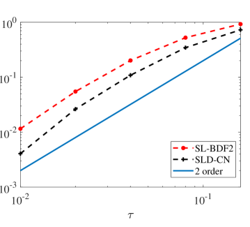
Figure 1: Temporal convergence of SLD-CN scheme and SL-BDF2 scheme.

Example 4.2.

We take initial value $\phi_{1}$ to test the spatial accuracy of the SLD-CN scheme. The Cahn-Hilliard equation with $\gamma=0.0025$ are solved from $t=0$ to $T=1$ with time step size $\tau=10^{-5}$. We take stability constants $A=0.025$ and $B=0.5$. To calculate the numerical error, we use the numerical result generated using $M=255$ as a reference of exact solution. Figure 2 presents the semilogy plot of errors in $H^{-1}$ norm, $L^{2}$ norm and $H^{1}$ norm against the polynomial degree $M=17,33,49,65,87$ for the SLD-CN scheme. We observe that the SLD-CN scheme in $H^{1}$ norm, $L^{2}$ norm and $H^{-1}$ norm are all spectral convergent. The convergence rate in $H^{-1}$ norm is higher than it in $H^{1}$ norm, which is as expected in Theorem 3.1.

Figure 2: Spatial convergence of SLD-CN scheme.

4.3 Adaptive time stepping

Several adaptive time stepping strategies have been implemented to Cahn-Hilliard equation. We propose an adaptive time-stepping strategy in which the time step is defined by the moving speed of the interface for SLD-CN scheme. The method is presented in Algorithm 4.1. We update the time step using the equation $A_{dp}(e_{n+1},\tau_{n+1})$, which is proposed by Gomez and Hughes [23]. Our default values for the safety coefficient $\rho$ and the tolerance $tol$ are given as $\rho=0.9$, $tol=10^{-3}$. The minimum and maximum time steps are taken as $\tau_{min}=10^{-6}$ and $\tau_{max}=0.01$, respectively. $e_{n+1}$ is the approximation of the relative ratio between the interface velocity and the interface thickness at the $(n+1)$th time level. The initial time step is taken as $10^{-3}$.

Algorithm 4.1.

Time step adaptive procedure:

• Step 1: Compute $\phi^{n+1}$ by SLD-CN scheme with $\tau_{n+1}$;
  

• Step 2: Calculate $E_{C}^{n+1}(\phi^{n+1},\phi^{n},B)$.
  

• Step 3: Calculate $e_{n+1}=10\left(\frac{\|\phi^{n+1}-\phi^{n}\|}{\varepsilon E_{C}^{n+1}(\phi^{n+1},\phi^{n},B)}\right)^{2}$ and
  $A_{dp}(e_{n+1},\tau_{n+1})=\rho\left(\frac{tol}{e_{n+1}}\right)^{1/2}\tau_{n+1};$

• Step 4: if $e_{n+1}>tol$, then
  recalculate time step: $\tau_{n+1}\leftarrow\max\{\tau_{min},\min\{A_{dp}(e_{n+1},\tau_{n+1}),\tau_{max}\}\}$;
  goto Step 1;
  else
  update time step size $\tau_{n+2}\leftarrow\min\{A_{dp}(e_{n+1},\tau_{n+1}),\tau_{max}\}$;
  continue to next time step.

We solve the Cahn-Hilliard equation with initial value $\phi_{0}$ and $M=63$ until $T=30$. We take $\gamma=0.0025$, $A=1$, $B=0.25$. We present numerical results of phase evolutions using large time steps, adaptive time steps, and small time steps for Cahn-Hilliard equation in Figure 4. We take a uniform large time step $\tau=0.01$ and a uniform small time step $\tau=10^{-5}$ for comparison. It is noted that the solutions by adaptive time steps in the second row are consistent with the solutions by uniform small time step in the third row. On the other hand, the uniform large time step solutions in the first row are far different from the adaptive time steps solutions. Figure 3 presents the adaptive time steps and discrete energy accordingly with the time. The time steps almost grow from $\tau=10^{-6}$ to $\tau=10^{-2}$. The last time step decreases because it is only 0.0034 from the second last step to the end time. Also, the discrete energy curve of adaptive time steps coincides with it of uniform small time steps $\tau=10^{-5}$, and does not coincide with that of uniform large time steps $\tau=0.01$. It indicates that the adaptive time stepping for the SLD-CN scheme is very effective.

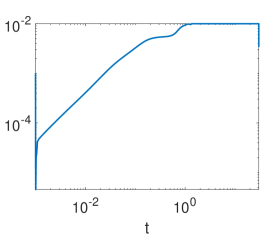
(a) Adaptive time step size.

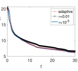
(b) Discrete energy.

Figure 3: Adaptive time steps and discrete energy against time until $T=30$.

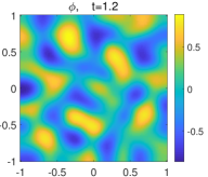
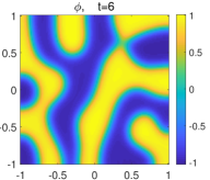
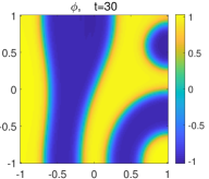
(a) $\tau=0.01$

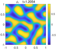
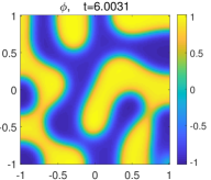
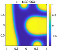
(b) Adaptive time steps

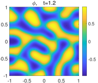
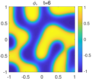
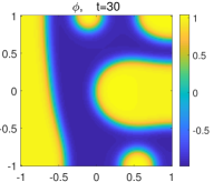
(c) $\tau=0.00001$

Figure 4: Numerical comparisons among large time steps, adaptive time steps, and small time steps for Cahn-Hilliard equation.

5 Conclusions

We propose the SLD-CN scheme by modifying the stabilized linear Crank-Nicolson scheme for the Cahn-Hilliard equation. In the scheme, the nonlinear bulk force is treated explicitly with two additional linear stabilization terms: $-A\tau\Delta\delta_{t}\phi^{n+1}$ and $B\delta_{tt}\phi^{n+1}$. We give a rigorous optimal error analysis of the fully discrete SLD-CN scheme, which removes the condition $B>L/2\varepsilon$ for the error analysis of the SL-CN scheme. This error analysis holds for the special case $A=0$ and/or $B=0$ as well. Numerical results verified the stability and accuracy of the proposed schemes.

Appendix A Estimate of the constants in Assumption 3.3

Lemma A.1.

Suppose Assumption 3.1 (i)-(iii) and Assumption 3.2 are satisfied. We have following regularity results for the exact solution $\phi$ of (2) with $\gamma=1$.

1. $\int_{0}^{\infty}\|\phi_{t}\|_{-1}^{2}{\rm d}t+\operatorname*{ess\,sup}\limits_{t\in[0,\infty]}E_{\varepsilon}(\phi)\lesssim\varepsilon^{-\beta_{1}}$, and $\|\phi\|_{H^{1}}^{2}\lesssim\varepsilon^{-(\sigma_{1}+1)}$;

2. $\operatorname*{ess\,sup}\limits_{t\in[0,\infty]}\|\phi_{t}\|_{-1}^{2}+\varepsilon\int_{0}^{\infty}\|\nabla\phi_{t}\|^{2}{\rm d}t\lesssim\varepsilon^{-\beta_{2}}$;

3. $\operatorname*{ess\,sup}\limits_{t\in[0,\infty]}\|\phi_{t}\|^{2}+\varepsilon\int_{0}^{\infty}\|\Delta\phi_{t}\|^{2}{\rm d}t\lesssim\varepsilon^{-\beta_{3}}$;

4. $\int_{0}^{\infty}\|\phi_{tt}\|_{-1}^{2}{\rm d}t+\operatorname*{ess\,sup}\limits_{t\in[0,\infty]}\varepsilon\|\nabla\phi_{t}\|^{2}\lesssim\varepsilon^{-\beta_{4}}$;

5. $\operatorname*{ess\,sup}\limits_{t\in[0,\infty]}\|\Delta^{-1}\phi_{tt}\|^{2}+\varepsilon\int_{0}^{\infty}\|\phi_{tt}\|^{2}{\rm d}t\lesssim\varepsilon^{-\beta_{5}}$;

6. $\operatorname*{ess\,sup}\limits_{t\in[0,\infty]}\|\phi_{tt}\|_{-1}^{2}+\varepsilon\int_{0}^{\infty}\|\nabla\phi_{tt}\|^{2}{\rm d}t\lesssim\varepsilon^{-\beta_{6}}$;

7. $\operatorname*{ess\,sup}\limits_{t\in[0,\infty]}\|\phi_{tt}\|^{2}+\varepsilon\int_{0}^{\infty}\|\Delta\phi_{tt}\|^{2}{\rm d}t\lesssim{}\varepsilon^{-\beta_{7}}$;

8. $\int_{0}^{\infty}\|\Delta^{-1}\phi_{tt}\|_{-1}^{2}{\rm d}t+\varepsilon\operatorname*{ess\,sup}\limits_{t\in[0,\infty]}\|\phi_{t}\|_{-1}^{2}\lesssim{}\varepsilon^{-\beta_{8}}$;

9. $\operatorname*{ess\,sup}\limits_{t\in[0,\infty]}\|\Delta^{-1}\phi_{t}\|^{2}+\varepsilon\int_{0}^{\infty}\|\phi_{t}\|^{2}{\rm d}t\lesssim{}\varepsilon^{-\beta_{9}}$;

10. $\int_{0}^{\infty}\|\phi_{t}\|_{H^{q+1}}^{2}{\rm d}t\lesssim{}\varepsilon^{-\beta_{10}}$, when $q=1$;

11. $\int_{0}^{\infty}\|\phi_{tt}\|_{H^{q+1}}^{2}{\rm d}t\lesssim{}\varepsilon^{-\beta_{11}}$, when $q=1$;

12. $\int_{0}^{T}\|\phi\|^{2}_{H^{2}}{\rm d}t\lesssim\varepsilon^{-(\sigma_{1}+3)}$;

13. $\int_{0}^{T}\|\mu\|^{2}_{H^{2}}{\rm d}t\lesssim\varepsilon^{-\beta_{12}}$.

where $\beta_{1}=\sigma_{1}$ and

$$\begin{split}\beta_{2}&=\max\{\sigma_{1}+3,\sigma_{2}\},\\ \beta_{3}&=\max\{(\sigma_{1}+1)(p-2)+\beta_{2}+4,\sigma_{3}\},\\ \beta_{4}&=\max\{\beta_{2}+2+\tfrac{1}{2}\beta_{3}+\tfrac{1}{2}(\sigma_{1}+1)(p-3)^{+},\sigma_{4}\},\\ \beta_{5}&=\max\{\beta_{2}+\beta_{4}+1+(\sigma_{1}+1)(p-3)^{+},(\sigma_{1}+1)(p-2)+\beta_{4}+3,\sigma_{5}\},\\ \beta_{6}&=\max\{(\sigma_{1}+1)(p-3)^{+}+\beta_{2}+\beta_{4}+5,\beta_{5}+2,\sigma_{6}\},\\ \beta_{7}&=\max\{(\sigma_{1}+1)(p-3)^{+}+\beta_{2}+\beta_{4}+5,(\sigma_{1}+1)(p-2)+\beta_{6}+4,\sigma_{7}\},\\ \beta_{8}&=\max\{(\sigma_{1}+1)(p-2)+\beta_{1}+2,(\sigma_{1}+1)(p-2)+\beta_{2}+3,\sigma_{2}+1\},\\ \beta_{9}&=(\sigma_{1}+1)(p-2)+\beta_{1}+3,\\ \beta_{10}&=\max\{\beta_{2}+1,\beta_{3}+1,\beta_{9}+1\},\\ \beta_{11}&=\max\{\beta_{5}+1,\beta_{6}+1,\beta_{7}+1\},\\ \beta_{12}&=\max\{\sigma_{1},(\sigma_{1}+1)(p-1)+3\}.\end{split}$$

Proof.

We first write down some inequalities that will be frequently used. The first one is the Holder’s inequality

$$\|uvw\|_{L^{s}}\leq\|u\|_{L^{p}}\|v\|_{L^{q}}\|w\|_{L^{r}},\quad\forall\ p,q,r\in(0,\infty],\ \frac{1}{s}=\frac{1}{p}+\frac{1}{q}+\frac{1}{r}.$$ (120)

The second one is the Sobolev inequality

$$\|u\|_{L^{q}}\leq C_{s}\|u\|_{1},$$ (121)

where $q\in[2,\infty)$ for $d=2$; $q\in[2,\frac{2d}{d-2}]$ for $d>2$; $C_{s}$ is a general constant independent of $\phi$. We can further use Poincare’s inequality to get

$$\|v\|_{L^{q}}\leq C_{s}\|\nabla v\|,\quad\forall v\in L^{2}_{0}(\Omega).$$ (122)

For $v\in L^{2}_{0}(\Omega)$, we also have following inequality

$$\|v\|^{2}=(\nabla v,\nabla(-\Delta)^{-1}v)\leq\frac{1}{2\delta}\|\nabla v\|^{2}+\frac{\delta}{2}\|v\|_{-1}^{2},$$ (123)

where $\delta>0$ is an arbitrary constant.

Now, we begin the proof.

1. When $\gamma=1$, we have Cahn-Hilliard equation

   $$\phi_{t}+\varepsilon\Delta^{2}\phi=\dfrac{1}{\varepsilon}\Delta f(\phi).$$ (124)

   Multiplying (124) by $-\Delta^{-1}\phi_{t}$ and using integration by parts, we get

   $$\|\phi_{t}\|_{-1}^{2}+\frac{\varepsilon}{2}\frac{d}{dt}\|\nabla\phi\|^{2}=-\frac{1}{\varepsilon}(f(\phi),\phi_{t})=-\frac{1}{\varepsilon}\frac{d}{dt}\int_{\Omega}F(\phi)dx.$$ (125)

   After integrating over $[0,T]$, we obtain

   $$\int_{0}^{T}\|\phi_{t}\|_{-1}^{2}{\rm d}t+E_{\varepsilon}(\phi(T))=E_{\varepsilon}(\phi^{0})$$ (126)

   Taking maximum values of terms on the left hand side for $T\in[0,\infty]$, we get the first part of (i) from (33). From the definition of $E_{\varepsilon}(\phi)$, and assumption (27) we know

   $$\|\phi\|^{2}\leq B_{0}|\Omega|+B_{1}\varepsilon^{-\sigma_{1}+1}\lesssim\varepsilon^{-(\sigma_{1}-1)^{+}}.$$ (127)

   Combining above estimate with the fact $\frac{\varepsilon}{2}\|\nabla\phi\|^{2}\lesssim\varepsilon^{-\sigma_{1}}$, we get

   $$\|\phi\|_{H^{1}}^{2}\lesssim\varepsilon^{-(\sigma_{1}+1)}.$$ (128)

2. We formally differentiate (124) in time to obtain

   $$\phi_{tt}+\varepsilon\Delta^{2}\phi_{t}=\dfrac{1}{\varepsilon}\Delta\left(f^{\prime}(\phi)\phi_{t}\right).\\$$ (129)

   Pairing (129) with $-\Delta^{-1}\phi_{t}$ and using (123), yields

   $$\begin{split}\frac{1}{2}\frac{d}{dt}\|\phi_{t}\|_{-1}^{2}+\varepsilon\|\nabla\phi_{t}\|^{2}=&-\dfrac{1}{\varepsilon}\left(f^{\prime}(\phi)\phi_{t},\phi_{t}\right)\leq\frac{\tilde{c}_{0}}{\varepsilon}\|\phi_{t}\|^{2}\\ \leq&\frac{\varepsilon}{2}\|\nabla\phi_{t}\|^{2}+\frac{\tilde{c}_{0}^{2}}{2\varepsilon^{3}}\|\phi_{t}\|_{-1}^{2}.\\ \end{split}$$ (130)

   Integrating (130) over $[0,T]$ and taking maximum values for terms depending on $T$, we get

   $$\operatorname*{ess\,sup}\limits_{t\in[0,\infty]}\|\phi_{t}\|_{-1}^{2}+\varepsilon\int_{0}^{\infty}\|\nabla\phi_{t}\|^{2}{\rm d}t\lesssim\frac{\tilde{c}_{0}^{2}}{\varepsilon^{3}}\int_{0}^{\infty}\|\phi_{t}\|_{-1}^{2}{\rm d}t+\|\phi_{t}^{0}\|_{-1}^{2}.\\$$ (131)

   The assertion then follows from (i) and the inequality (34) of Assumption 3.2.

3. Testing (129) with $\phi_{t}$, using (120) and (121) with Poincare’s inequality, we get

   $$\begin{split}\frac{1}{2}\frac{d}{dt}\|\phi_{t}\|^{2}+\varepsilon\|\Delta\phi_{t}\|^{2}=&\frac{1}{\varepsilon}(f^{\prime}(\phi)\phi_{t},\Delta\phi_{t})\leq\frac{1}{\varepsilon}\|f^{\prime}(\phi)\|_{L^{3}}\|\phi_{t}\|_{L^{6}}\|\Delta\phi_{t}\|\\ \leq&\frac{\varepsilon}{2}\|\Delta\phi_{t}\|^{2}+\frac{1}{2\varepsilon^{3}}\|f^{\prime}(\phi)\|_{L^{3}}^{2}\|\phi_{t}\|_{L^{6}}^{2}\\ \leq&\frac{\varepsilon}{2}\|\Delta\phi_{t}\|^{2}+\frac{C_{s}^{2}}{2\varepsilon^{3}}\|f^{\prime}(\phi)\|_{L^{3}}^{2}\|\nabla\phi_{t}\|^{2},\end{split}$$ (132)

   which leads to

   $$\begin{split}&\operatorname*{ess\,sup}\limits_{t\in[0,\infty]}\|\phi_{t}\|^{2}+\varepsilon\int_{0}^{\infty}\|\Delta\phi_{t}\|^{2}{\rm d}t\\ \lesssim&\frac{C_{s}}{\varepsilon^{3}}\operatorname*{ess\,sup}_{t\in[0,\infty]}\|f^{\prime}(\phi)\|_{L^{3}}^{2}\int_{0}^{\infty}\|\nabla\phi_{t}\|^{2}{\rm d}t+\|\phi_{t}^{0}\|^{2}.\end{split}$$ (133)

   On the other hand side, by assumption (29), the Sobolev inequality (121) and estimate (128), we have

   $$\|f^{\prime}(\phi)\|_{L^{3}}^{2}\lesssim\tilde{c}_{2}\|\phi\|_{L^{3(p-2)}}^{2(p-2)}+\tilde{c}_{3}\lesssim\tilde{c}_{2}\|\phi\|_{1}^{2(p-2)}+\tilde{c}_{3}\lesssim\varepsilon^{-(\sigma_{1}+1)(p-2)}$$ (134)

   The assertion then follows from (133), (134), (ii) and assumption (35).

4. Testing (129) with $-\Delta^{-1}\phi_{tt}$, we get

   $$\begin{split}&\|\phi_{tt}\|_{-1}^{2}+\frac{\varepsilon}{2}\frac{d}{dt}\|\nabla\phi_{t}\|^{2}=-\dfrac{1}{\varepsilon}(f^{\prime}(\phi)\phi_{t},\phi_{tt})\\ =&-\frac{1}{2\varepsilon}\frac{d}{dt}(f^{\prime}(\phi)\phi_{t},\phi_{t})+\frac{1}{2\varepsilon}(f^{\prime\prime}(\phi)\phi_{t}^{2},\phi_{t})\\ \leq&-\frac{1}{2\varepsilon}\frac{d}{dt}(f^{\prime}(\phi)\phi_{t},\phi_{t})+\frac{1}{2\varepsilon}\|f^{\prime\prime}\|_{L^{6}}\|\phi_{t}^{2}\|_{L^{3}}\|\phi_{t}\|\\ \leq&-\frac{1}{2\varepsilon}\frac{d}{dt}(f^{\prime}(\phi)\phi_{t},\phi_{t})+\frac{C_{s}^{2}}{2\varepsilon}\|f^{\prime\prime}\|_{L^{6}}\|\nabla\phi_{t}\|^{2}\|\phi_{t}\|\\ \end{split}$$ (135)

   Integrate (135) over $[0,T]$, we continue the estimate as

   $$\begin{split}&2\int_{0}^{T}\|\phi_{tt}\|_{-1}^{2}{\rm d}t+\varepsilon\|\nabla\phi_{t}(T)\|^{2}-\varepsilon\|\nabla\phi_{t}^{0}\|^{2}\\ \leq&-\frac{1}{\varepsilon}(f^{\prime}(\phi)\phi_{t},\phi_{t})|_{t=T}+\frac{1}{\varepsilon}(f^{\prime}(\phi^{0})\phi_{t}^{0},\phi_{t}^{0})\\ &+\frac{C_{s}^{2}}{\varepsilon}\operatorname*{ess\,sup}_{t\in[0,T]}\{\|f^{\prime\prime}\|_{L^{6}}\|\phi_{t}\|\}\int_{0}^{T}\|\nabla\phi_{t}\|^{2}{\rm d}t\\ \leq&\frac{\varepsilon}{2}\|\nabla\phi_{t}(T)\|^{2}+\frac{\tilde{c}_{0}^{2}}{2\varepsilon^{3}}\|\phi_{t}(T)\|_{-1}^{2}+\frac{1}{\varepsilon}(f^{\prime}(\phi^{0})\phi_{t}^{0},\phi_{t}^{0})\\ &+\frac{C_{s}^{2}}{\varepsilon}\operatorname*{ess\,sup}_{t\in[0,T]}\{\|f^{\prime\prime}\|_{L^{6}}\|\phi_{t}\|\}\int_{0}^{T}\|\nabla\phi_{t}\|^{2}{\rm d}t,\end{split}$$ (136)

   i.e.

   $$\begin{split}2\int_{0}^{T}\|\phi_{tt}\|_{-1}^{2}{\rm d}t&+\frac{\varepsilon}{2}\|\nabla\phi_{t}(T)\|^{2}\leq\varepsilon\|\nabla\phi_{t}^{0}\|^{2}+\frac{1}{\varepsilon}(f^{\prime}(\phi^{0})\phi_{t}^{0},\phi_{t}^{0})\\ &+\frac{\tilde{c}_{0}^{2}}{2\varepsilon^{3}}\|\phi_{t}(T)\|_{-1}^{2}+\frac{C_{s}^{2}}{\varepsilon}\operatorname*{ess\,sup}_{t\in[0,T]}\{\|f^{\prime\prime}\|_{L^{6}}\|\phi_{t}\|\}\int_{0}^{T}\|\nabla\phi_{t}\|^{2}{\rm d}t.\end{split}$$ (137)

   On the other hand, by (30), the Sobolev inequality (121) and estimate (128), we have

   $$\|f^{\prime\prime}(\phi)\|_{L^{6}}^{2}\lesssim\tilde{c}_{4}\|\phi\|_{L^{6(p-3)^{+}}}^{2(p-3)^{+}}+\tilde{c}_{5}\lesssim\|\phi\|_{1}^{2(p-3)^{+}}\lesssim\varepsilon^{-(\sigma_{1}+1)(p-3)^{+}}$$ (138)

   By taking maximum for terms depending on $T$ in (137) and using (138), (ii), (iii) and the inequality (36) of Assumption 3.2. we obtain the assertion (iv).

5. We formally differentiate (129) in time to derive

   $$\phi_{ttt}+\varepsilon\Delta^{2}\phi_{tt}=\dfrac{1}{\varepsilon}\Delta\left(f^{\prime\prime}(\phi)(\phi_{t})^{2}+f^{\prime}(\phi)\phi_{tt}\right).\\$$ (139)

   Testing (139) with $\Delta^{-2}\phi_{tt}$, we obtain

   $$\begin{split}&\frac{1}{2}\frac{d}{dt}\|\Delta^{-1}\phi_{tt}\|^{2}+\varepsilon\|\phi_{tt}\|^{2}=\dfrac{1}{\varepsilon}\left(f^{\prime\prime}(\phi)(\phi_{t})^{2}+f^{\prime}(\phi)\phi_{tt},\Delta^{-1}\phi_{tt}\right)\\ \leq{}&\dfrac{\varepsilon}{2}\|f^{\prime\prime}(\phi)\|^{2}_{L^{2}}\|\phi_{t}\|_{L^{6}}^{4}+\dfrac{1}{2\varepsilon^{3}}\|\Delta^{-1}\phi_{tt}\|^{2}_{L^{6}}+\frac{1}{2\varepsilon^{3}}\|f^{\prime}(\phi)\|_{L^{3}}^{2}\|\Delta^{-1}\phi_{tt}\|_{L^{6}}^{2}+\frac{\varepsilon}{2}\|\phi_{tt}\|^{2}\\ \leq{}&\dfrac{\varepsilon}{2}C_{s}^{4}\|f^{\prime\prime}(\phi)\|^{2}_{L^{2}}\|\nabla\phi_{t}\|^{4}+\dfrac{C_{s}^{2}}{2\varepsilon^{3}}\|\phi_{tt}\|^{2}_{-1}+\frac{C_{s}^{2}}{2\varepsilon^{3}}\|f^{\prime}(\phi)\|_{L^{3}}^{2}\|\phi_{tt}\|_{-1}^{2}+\frac{\varepsilon}{2}\|\phi_{tt}\|^{2}.\\ \end{split}$$ (140)

   After taking integration from $[0,T]$ and taking maximum for terms depending on $T$, we have

   $$\begin{split}&\operatorname*{ess\,sup}\limits_{t\in[0,\infty]}\|\Delta^{-1}\phi_{tt}\|^{2}+\varepsilon\int_{0}^{\infty}\|\phi_{tt}\|^{2}{\rm d}t\\ \lesssim{}&{\varepsilon}\operatorname*{ess\,sup}\limits_{t\in[0,\infty]}\left(\|f^{\prime\prime}(\phi)\|^{2}_{L^{2}}\|\nabla\phi_{t}\|^{2}\right)\int_{0}^{\infty}\|\nabla\phi_{t}\|^{2}{\rm d}t\\ &+\frac{1}{\varepsilon^{3}}\left(\operatorname*{ess\,sup}_{t\in[0,\infty]}\|f^{\prime}(\phi)\|_{L^{3}}^{2}+1\right)\int_{0}^{\infty}\|\phi_{tt}\|^{2}_{-1}{\rm d}t+\|\Delta^{-1}\phi_{tt}^{0}\|^{2}.\\ \end{split}$$ (141)

   The assertion then follows from (134), the following estimate

   $$\|f^{\prime\prime}(\phi)\|_{L^{2}}^{2}\lesssim\tilde{c}_{4}\|\phi\|_{L^{2(p-3)^{+}}}^{2(p-3)^{+}}+\tilde{c}_{5}\lesssim\|\phi\|_{1}^{2(p-3)^{+}}\lesssim\varepsilon^{-(\sigma_{1}+1)(p-3)^{+}},$$ (142)

   (ii), (iv) and the inequality (37) of Assumption 3.2.

6. Pairing (139) with $-\Delta^{-1}\phi_{tt}$, we obtain

   $$\begin{split}&\frac{\varepsilon}{2}\frac{d}{dt}\|\phi_{tt}\|_{-1}^{2}+\varepsilon\|\nabla\phi_{tt}\|^{2}\\ =&-\dfrac{1}{\varepsilon}\left(f^{\prime\prime}(\phi)(\phi_{t})^{2}+f^{\prime}(\phi)\phi_{tt},\phi_{tt}\right)\\ \leq&\dfrac{C_{s}^{2}}{2\varepsilon^{3}}\|f^{\prime\prime}(\phi)\|_{L^{2}}^{2}\|\phi_{t}\|_{L^{6}}^{4}+\frac{\varepsilon}{2C_{s}^{2}}\|\phi_{tt}\|_{L^{6}}^{2}+\frac{\tilde{c}_{0}}{\varepsilon}\|\phi_{tt}\|^{2}\\ \leq&\dfrac{C_{s}^{6}}{2\varepsilon^{3}}\|f^{\prime\prime}(\phi)\|_{L^{2}}^{2}\|\nabla\phi_{t}\|^{4}+\frac{\varepsilon}{2}\|\nabla\phi_{tt}\|^{2}+\frac{\tilde{c}_{0}}{\varepsilon}\|\phi_{tt}\|^{2}.\\ \end{split}$$ (143)

   Integrating (143) from $[0,\infty)$, we have

   $$\begin{split}&\operatorname*{ess\,sup}\limits_{t\in[0,\infty]}\|\phi_{tt}\|_{-1}^{2}+\varepsilon\int_{0}^{\infty}\|\nabla\phi_{tt}\|^{2}{\rm d}t\\ \lesssim{}&\frac{C_{s}^{6}}{\varepsilon^{3}}\operatorname*{ess\,sup}\limits_{t\in[0,\infty]}\left(\|f^{\prime\prime}(\phi)\|^{2}_{L^{2}}\|\nabla\phi_{t}\|^{2}\right)\int_{0}^{\infty}\|\nabla\phi_{t}\|^{2}{\rm d}t\\ &+\frac{2\tilde{c}_{0}}{\varepsilon}\int_{0}^{\infty}\|\phi_{tt}\|^{2}{\rm d}t+\|\phi_{tt}^{0}\|_{-1}^{2}.\\ \end{split}$$ (144)

   The assertion then follows from (142), (ii), (iv), (vi) and the inequality (38) of Assumption 3.2.

7. Pairing (139) with $\phi_{tt}$, we obtain

   $$\begin{split}&\frac{1}{2}\frac{d}{dt}\|\phi_{tt}\|^{2}+\varepsilon\|\Delta\phi_{tt}\|^{2}\\ =&\dfrac{1}{\varepsilon}\left(f^{\prime\prime}(\phi)(\phi_{t})^{2}+f^{\prime}(\phi)\phi_{tt},\Delta\phi_{tt}\right)\\ \leq&\frac{1}{\varepsilon}\|f^{\prime\prime}(\phi)\|_{L^{6}}\|\phi_{t}^{2}\|_{L^{3}}\|\Delta\phi_{tt}\|+\frac{1}{\varepsilon}\|f^{\prime}(\phi)\|_{L^{3}}\|\phi_{tt}\|_{L^{6}}\|\Delta\phi_{tt}\|\\ \leq&\dfrac{1}{\varepsilon^{3}}\left(\|f^{\prime\prime}(\phi)\|_{L^{6}}^{2}\|\phi_{t}\|_{L^{6}}^{4}+\|f^{\prime}(\phi)\|_{L^{3}}^{2}\|\phi_{tt}\|_{L^{6}}^{2}\right)+\frac{\varepsilon}{2}\|\Delta\phi_{tt}\|^{2}\\ \leq&\dfrac{1}{\varepsilon^{3}}\left(C_{s}^{4}\|f^{\prime\prime}(\phi)\|_{L^{6}}^{2}\|\nabla\phi_{t}\|^{4}+C_{s}^{2}\|f^{\prime}(\phi)\|_{L^{3}}^{2}\|\nabla\phi_{tt}\|^{2}\right)+\frac{\varepsilon}{2}\|\Delta\phi_{tt}\|^{2}.\\ \end{split}$$ (145)

   After taking integration from $[0,T]$ and taking maximum for terms depending on $T$, we have

   $$\begin{split}&\operatorname*{ess\,sup}\limits_{t\in[0,\infty]}\|\phi_{tt}\|^{2}+\varepsilon\int_{0}^{\infty}\|\Delta\phi_{tt}\|^{2}{\rm d}t\\ \lesssim{}&\frac{2C_{s}^{4}}{\varepsilon^{3}}\operatorname*{ess\,sup}\limits_{t\in[0,\infty]}\left(\|f^{\prime\prime}(\phi)\|^{2}_{L^{6}}\|\nabla\phi_{t}\|^{2}\right)\int_{0}^{\infty}\|\nabla\phi_{t}\|^{2}{\rm d}t\\ &+\frac{2C_{s}^{2}}{\varepsilon^{3}}\operatorname*{ess\,sup}_{t\in[0,\infty]}\|f^{\prime}(\phi)\|_{L^{3}}^{2}\int_{0}^{\infty}\|\nabla\phi_{tt}\|^{2}{\rm d}t+\|\phi_{tt}^{0}\|^{2}.\\ \end{split}$$ (146)

   The assertion then follows from (138), (134), (ii), (iv), (v) and the inequality (39) of Assumption 3.2.

8. Pairing (129) with $-\Delta^{-3}\phi_{tt}$, we obtain

   $$\begin{split}&\|\Delta^{-1}\phi_{tt}\|_{-1}^{2}+\frac{\varepsilon}{2}\frac{d}{dt}\|\phi_{t}\|_{-1}^{2}\\ =&-\dfrac{1}{\varepsilon}(f^{\prime}(\phi)\phi_{t},\Delta^{-2}\phi_{tt})\leq\frac{1}{\varepsilon}\|f^{\prime}(\phi)\|_{L^{3}}\|\phi_{t}\|\|\Delta^{-2}\phi_{tt}\|_{L^{6}}\\ \leq&\frac{1}{2C_{s}^{2}}\|\Delta^{-2}\phi_{tt}\|_{L^{6}}^{2}+\frac{C_{s}^{2}}{2\varepsilon^{2}}\|f^{\prime}(\phi)\|_{L^{3}}^{2}\|\phi_{t}\|^{2}\\ \leq&\frac{1}{2}\|\Delta^{-1}\phi_{tt}\|_{-1}^{2}+\frac{C_{s}^{2}}{2\varepsilon^{2}}\|f^{\prime}(\phi)\|_{L^{3}}^{2}(\|\phi_{t}\|_{-1}^{2}+\|\nabla\phi_{t}\|^{2}).\end{split}$$ (147)

   After taking integration from $[0,T]$ and taking maximum for terms depending on $T$, we have

   $$\begin{split}&\int_{0}^{\infty}\|\Delta^{-1}\phi_{tt}\|_{-1}^{2}{\rm d}t+\varepsilon\operatorname*{ess\,sup}\limits_{t\in[0,\infty]}\|\phi_{t}\|_{-1}^{2}\\ \lesssim{}&\frac{C_{s}^{2}}{\varepsilon^{2}}\operatorname*{ess\,sup}\limits_{t\in[0,\infty]}\|f^{\prime}(\phi)\|_{L^{3}}^{2}\int_{0}^{\infty}(\|\phi_{t}\|_{-1}^{2}+\|\nabla\phi_{t}\|^{2}){\rm d}t+\varepsilon\|\phi_{t}^{0}\|_{-1}^{2}.\end{split}$$ (148)

   The assertion then follows from (134), (i), (ii) and the inequality (34) of Assumption 3.2.

9. Pairing (129) with $\Delta^{-2}\phi_{t}$, we obtain

   $$\begin{split}&\frac{1}{2}\frac{d}{dt}\|\Delta^{-1}\phi_{t}\|^{2}+\varepsilon\|\phi_{t}\|^{2}\\ =&\dfrac{1}{\varepsilon}(f^{\prime}(\phi)\phi_{t},\Delta^{-1}\phi_{t})\leq\frac{1}{\varepsilon}\|f^{\prime}(\phi)\|_{L^{3}}\|\phi_{t}\|\|\Delta^{-1}\phi_{t}\|_{L^{6}}\\ \leq&\frac{\varepsilon}{2}\|\phi_{t}\|^{2}+\frac{C_{s}^{2}}{2\varepsilon^{3}}\|f^{\prime}(\phi)\|_{L^{3}}^{2}\|\phi_{t}\|_{-1}^{2}.\end{split}$$ (149)

   After taking integration from $[0,T]$ and taking maximum for terms depending on $T$, we have

   $$\begin{split}&\operatorname*{ess\,sup}\limits_{t\in[0,\infty]}\|\Delta^{-1}\phi_{t}\|^{2}+\varepsilon\int_{0}^{\infty}\|\phi_{t}\|^{2}{\rm d}t\\ \leq&\frac{C_{s}^{2}}{\varepsilon^{3}}\operatorname*{ess\,sup}\limits_{t\in[0,\infty]}\|f^{\prime}(\phi)\|_{L^{3}}^{2}\int_{0}^{\infty}\|\phi_{t}\|_{-1}^{2}{\rm d}t.\end{split}$$ (150)

10. We can easily get the proof from (ii) (iii) (ix).

11. We can easily get the proof from (v) (vi) (vii).

12. Multiplying (124) by $\phi$ and using integration by parts and $\frac{\varepsilon}{2}\|\nabla\phi\|^{2}\lesssim\varepsilon^{-\sigma_{1}}$, we get

    $$\begin{split}&\frac{1}{2}\frac{d}{dt}\|\phi\|^{2}+\varepsilon\|\Delta\phi\|^{2}=\frac{1}{\varepsilon}(\Delta f(\phi),\phi)\\ =&-\frac{1}{\varepsilon}(f^{\prime}(\phi)\nabla\phi,\nabla\phi)\leq\frac{\tilde{c}_{0}}{\varepsilon}\|\nabla\phi\|^{2}\lesssim\varepsilon^{-(\sigma_{1}+2)}.\end{split}$$ (151)

    Then we easily get

    $$\begin{split}\int_{0}^{T}\|\phi\|^{2}_{H^{2}}{\rm d}t\lesssim\int_{0}^{T}\|\phi\|^{2}+\|\nabla\phi\|^{2}+\|\Delta\phi\|^{2}{\rm d}t\lesssim\varepsilon^{-(\sigma_{1}+3)}.\end{split}$$ (152)

13. Multiplying (124) by $\Delta^{-1}\phi_{t}$ and using integration by parts, we get

    $$\begin{split}&\|\Delta^{-1}\phi_{t}\|^{2}+\frac{\varepsilon}{2}\frac{d}{dt}\|\phi\|^{2}=\frac{1}{\varepsilon}(f(\phi),\Delta^{-1}\phi_{t})\\ =&-\frac{1}{\varepsilon}(f^{\prime}(\phi)\nabla\phi,\Delta^{-\frac{3}{2}}\phi_{t})\leq\frac{1}{\varepsilon}\|f^{\prime}(\phi)\|_{L^{3}}\|\nabla\phi\|\|\Delta^{-\frac{3}{2}}\phi_{t}\|_{L^{6}}\\ \leq&\frac{1}{2C_{s}^{2}}\|\Delta^{-\frac{3}{2}}\phi_{t}\|_{L^{6}}^{2}+\frac{C_{s}^{2}}{2\varepsilon^{2}}\|f^{\prime}(\phi)\|_{L^{3}}^{2}\|\nabla\phi\|^{2}\\ \leq&\frac{1}{2}\|\Delta^{-1}\phi_{t}\|^{2}+\frac{C_{s}^{2}}{2\varepsilon^{2}}\|f^{\prime}(\phi)\|_{L^{3}}^{2}\|\nabla\phi\|^{2}.\end{split}$$ (153)

    After taking integration from $[0,T]$, we have

    $$\begin{split}&\int_{0}^{T}\|\Delta^{-1}\phi_{t}\|^{2}{\rm d}t+\varepsilon\operatorname*{ess\,sup}\limits_{t\in[0,T]}\|\phi\|^{2}\\ \leq&\frac{C_{s}^{2}}{\varepsilon^{2}}\operatorname*{ess\,sup}\limits_{t\in[0,T]}\|f^{\prime}(\phi)\|_{L^{3}}^{2}\int_{0}^{T}\|\nabla\phi\|^{2}{\rm d}t\lesssim\varepsilon^{-(\sigma_{1}+1)(p-1)-2}.\end{split}$$ (154)

    On the other hand

    $$\phi_{t}=\Delta\mu,$$ (155)

    combining above estimate with (i) (ix), then we have

    $$\int_{0}^{T}\|\mu\|^{2}_{H^{2}}{\rm d}t\lesssim\int_{0}^{T}\|\Delta^{-1}\phi_{t}\|^{2}+\|\phi_{t}\|_{-1}^{2}+\|\phi_{t}\|^{2}{\rm d}t\lesssim\varepsilon^{-\beta_{12}}.$$ (156)

∎

References

References

[1]
Nicholas D. Alikakos, Peter W. Bates, and Xinfu Chen.
Convergence of the Cahn-Hilliard equation to the Hele-Shaw
model.
Arch. Ration. Mech. Anal., 128(2):165–205, 1994.
[2]
D. M Anderson, G. B Mcfadden, and A. A Wheeler.
Diffuse-Interface Methods in Fluid Mechanics.
Annu. rev. fluid Mech, 30(1):139–165, 2003.
[3]
A. Baskaran, P. Zhou, Z. Hu, C. Wang, S. Wise, and J. Lowengrub.
Energy stable and efficient finite-difference nonlinear multigrid
schemes for the modified phase field crystal equation.
J. Comput. Phys., 250:270–292, 2013.
[4]
S. Brenner and L. Scott.
The Mathematical Theory of Finite Element Methods.Springer-Verlag, 2010.
[5]
Luis A. Caffarelli and Nora E. Muler.
An bound for solutions of the Cahn-Hilliard
equation.
Arch. Ration. Mech. Anal., 133(2):129–144, 1995.
[6]
John W. Cahn and John E. Hilliard.
Free energy of a nonuniform system. I. interfacial free energy.
J. Chem. Phys., 28(2):258–267, 1958.
[7]
Xinfu Chen.
Spectrum for the Allen-Cahn, Cahn-Hillard, and phase-field
equations for generic interfaces.
Commun. Part. Diff. Eq., 19(7):1371–1395, 1994.
[8]
Kelong Cheng, Cheng Wang, Steven M. Wise, and Xingye Yue.
A Second-Order, Weakly Energy-Stable Pseudo-spectral
Scheme for the Cahn-Hilliard Equation and Its Solution by the
Homogeneous Linear Iteration Method.
J. Sci. Comput., 69(3):1083–1114, 2016.
[9]
Nicolas Condette, Christof Melcher, and Endre Süli.
Spectral approximation of pattern-forming nonlinear evolution
equations with double-well potentials of quadratic growth.
Math. Comp., 80(273):205–223, 2011.
[10]
Amanda E. Diegel, Cheng Wang, and Steven M. Wise.
Stability and convergence of a second order mixed finite element
method for the Cahn-Hilliard equation.
IMA J Numer. Anal., 36(4):1867–1897, 2016.
[11]
Qiang Du and Roy A. Nicolaides.
Numerical analysis of a continuum model of phase transition.
SIAM J. Numer. Anal., 28(5):1310–1322, 1991.
[12]
C. M. Elliott and A. M. Stuart.
The global dynamics of discrete semilinear parabolic equations.
SIAM J. Numer. Anal., 30:1622–1663, 1993.
[13]
Charles M. Elliott and Harald Garcke.
On the Cahn-Hilliard Equation with Degenerate Mobility.
SIAM J. Math. Anal., 27(2):404–423, 1996.
[14]
Charles M. Elliott and Stig Larsson.
Error estimates with smooth and nonsmooth data for a finite element
method for the Cahn-Hilliard equation.
Math. Comp., 58(198):603–630, S33–S36, 1992.
[15]
D. J. Eyre.
Unconditionally gradient stable time marching the Cahn-Hilliard
equation.
In Computational and Mathematical Models of Microstructural
Evolution (San Francisco, CA, 1998), volume 529 of Mater. Res.
Soc. Sympos. Proc., pages 39–46. MRS, 1998.
[16]
Xiaobing Feng and Yukun Li.
Analysis of symmetric interior penalty discontinuous Galerkin
methods for the Allen-Cahn equation and the mean curvature flow.
IMA J. Numer. Anal., 35(4):1622–1651, 2015.
[17]
Xiaobing Feng, Yukun Li, and Yulong Xing.
Analysis of mixed interior penalty discontinuous Galerkin methods
for the Cahn-Hilliard equation and the Hele-Shaw flow.
SIAM J. Numer. Anal., 54(2):825–847, 2016.
[18]
Xiaobing Feng and Andreas Prohl.
Numerical analysis of the Allen-Cahn equation and approximation
for mean curvature flows.
Numer. Math., 94(1):33–65, 2003.
[19]
Xiaobing Feng and Andreas Prohl.
Error analysis of a mixed finite element method for the
Cahn-Hilliard equation.
Numer. Math., 99(1):47–84, 2004.
[20]
Xiaobing Feng and Andreas Prohl.
Numerical analysis of the Cahn-Hilliard equation and
approximation for the Hele-Shaw problem.
Interfaces Free Bound., 7(1):1–28, 2005.
[21]
Xinlong Feng, Tao Tang, and Jiang Yang.
Stabilized Crank-Nicolson/Adams-Bashforth schemes for phase
field models.
E. Asian J. Appl. Math., 3(1):59–80, 2013.
[22]
Daisuke Furihata.
A stable and conservative finite difference scheme for the
Cahn-Hlliard equation.
Numer. Math., 87(4):675–699, 2001.
[23]
Hector Gomez and Thomas J. R. Hughes.
Provably unconditionally stable, second-order time-accurate, mixed
variational methods for phase-field models.
J. Comput. Phys., 230(13):5310–5327, 2011.
[24]
F. Guillén-González and G. Tierra.
On linear schemes for a Cahn-Hilliard diffuse interface model.
J. Comput. Phys., 234:140–171, 2013.
[25]
Francisco Guillén-González and Giordano Tierra.
Second order schemes and time-step adaptivity for Allen-Cahn and
Cahn-Hilliard models.
Comput. Math. Appl., 68(8):821–846, 2014.
[26]
Jing Guo, Cheng Wang, Steven M. Wise, and Xingye Yue.
An convergence of a second-order convex-splitting, finite
difference scheme for the three-dimensional Cahn-Hilliard equation.
Commun. Math. Sci, 14(2):489–515, 2016.
[27]
D. Han, A. Brylev, X. Yang, and Z. Tan.
Numerical analysis of second order, fully discrete energy stable
schemes for phase field models of two phase incompressible flows.
J. Sci. Comput., 70:965–989, 2017.
[28]
Yinnian He, Yunxian Liu, and Tao Tang.
On large time-stepping methods for the Cahn-Hilliard equation.
Appl. Numer. Math., 57(5-7):616–628, 2007.
[29]
Daniel Kessler, Ricardo H. Nochetto, and Alfred Schmidt.
A posteriori error control for the Allen-Cahn problem:
circumventing Gronwall’s inequality.
ESAIM: Math. Model. Numer. Anal., 38(01):129–142, 2004.
[30]
Dong Li and Zhonghua Qiao.
On second order semi-implicit Fourier spectral methods for 2d
Cahn-Hilliard equations.
J. Sci. Comput., 70(1):301–341, 2017.
[31]
Dong Li, Zhonghua Qiao, and Tao Tang.
Characterizing the stabilization size for semi-implicit
Fourier-spectral method to phase field equations.
SIAM J Numer. Anal., 54(3):1653–1681, 2016.
[32]
Weijia Li, Wenbin Chen, Cheng Wang, Yue Yan, and Ruijian He.
A second order energy stable linear scheme for a thin film model
without slope selection.
J. Sci. Comput., 76(3):1905–1937, 2018.
[33]
Xiao Li, Zhonghua Qiao, and Hui Zhang.
A second-order convex splitting scheme for a Cahn-Hilliard
equation with variable interfacial parameters.
J. Comput. Math., 35(6):693–710, 2017.
[34]
Chun Liu and Jie Shen.
A phase field model for the mixture of two incompressible fluids and
its approximation by a Fourier-spectral method.
Physica D, 179(3-4):211–228, 2003.
[35]
Jie Shen.
Efficient spectral-galerkin method ii. direct solvers of second- and
fourth-order equations using chebyshev polynomials.
SIAM J. Sci. Comput., 16:74–87, 1995.
[36]
Jie Shen, Jie Xu, and Jiang Yang.
The scalar auxiliary variable (SAV) approach for gradient flows.
J. Comput. Phys., 353:407–416, 2018.
[37]
Jie Shen, Jie Xu, and Jiang Yang.
A new class of efficient and robust energy stable schemes for
gradient flows.
SIAM Rev., 61(3):474–506, 2019.
[38]
Jie Shen and Xiaofeng Yang.
Numerical approximations of Allen-Cahn and Cahn-Hilliard
equations.
Discrete Cont. Dyn. A, 28:1669–1691, 2010.
[39]
Jie Shen, Xiaofeng Yang, and Haijun Yu.
Efficient energy stable numerical schemes for a phase field moving
contact line model.
J. Comput. Phys., 284:617–630, 2015.
[40]
Lin Wang and Haijun Yu.
Convergence analysis of an unconditionally energy stable linear
Crank-Nicolson scheme for the Cahn-Hilliard equation.
J. Math. Study, 51(1):89–114, 2018.
[41]
Lin Wang and Haijun Yu.
On efficient second order stabilized semi-implicit schemes for the
Cahn-Hilliard phase-field equation.
J. Sci. Comput., 77(2):1185–1209, 2018.
[42]
Lin Wang and Haijun Yu.
Energy stable second order linear schemes for the Allen-Cahn
phase-field equation.
Commun. Math. Sci., 17(3):609–635, 2019.
[43]
X. Wu, G. J. van Zwieten, and K. G. van der Zee.
Stabilized second-order convex splitting schemes for
Cahn-Hilliard models with application to diffuse-interface tumor-growth
models.
Int. J. Numer. Meth. Biomed. Engng., 30(2):180–203, 2014.
[44]
Yue Yan, Wenbin Chen, Cheng Wang, and Steven Wise.
A second-order energy stable BDF numerical scheme for the
Cahn-Hilliard equation.
Commun. Comput. Phys., 23(2):572–602, 2018.
[45]
Xiaofeng Yang.
Error analysis of stabilized semi-implicit method of Allen-Cahn
equation.
Discrete. Cont. Dyn. B., 11(4):1057–1070, 2009.
[46]
Xiaofeng Yang.
Linear, first and second-order, unconditionally energy stable
numerical schemes for the phase field model of homopolymer blends.
J. Comput. Phys., 327:294–316, 2016.
[47]
Xiaofeng Yang and Lili Ju.
Efficient linear schemes with unconditional energy stability for the
phase field elastic bending energy model.
Comput. Method. Appl. Mech. Eng., 315:691–712, 2017.
[48]
Xiaofeng Yang and Haijun Yu.
Efficient second order unconditionally stable schemes for a phase
field moving contact line model using an invariant energy quadratization
approach.
SIAM J. Sci. Comput., 40(3):B889–B914, 2018.
[49]
Pengtao Yue, James J. Feng, Chun Liu, and Jie Shen.
A diffuse-interface method for simulating two-phase flows of complex
fluids.
J. Fluid. Mech., 515:293–317, 2004.