Quantifying the Effect of Power Spectral Density Uncertainty on Gravitational-Wave Parameter Estimation for Compact Binary Sources

Abstract

In order to perform Bayesian parameter estimation to infer the source properties of gravitational waves from compact binary coalescences, the noise characteristics of the detector must be understood. It is typically assumed that the detector noise is stationary and Gaussian, characterized by a power spectral density (PSD) that is measured with infinite precision. We present a new method to incorporate the uncertainty in the power spectral density estimation into the Bayesian inference of the binary source parameters and apply it to the first 11 CBC detections reported by the LIGO-Virgo Collaboration. We find that incorporating the PSD uncertainty only leads to variations in the positions and widths of the binary parameter posteriors on the order of a few percent. Our results are publicly available for download on git dat .

I Introduction

A gravitational wave detector, such as the ground-based laser interferometers LIGO and Virgo Aasi et al. (2015); Acernese et al. (2015), is assumed to generate an output consisting of background Gaussian noise. Gravitational-wave signals, as well as non-Gaussian noise transients, will introduce a deviation of the detector output from the baseline noise behavior. As the sensitivity of the network of ground-based laser interferometers searching for gravitational waves improves Abbott et al. (2018a), so too must our understanding of their noise properties. These noise properties are usually characterized by the power spectral density (PSD) in each detector, which is a required input for both low latency searches for gravitational waves and further source characterization via Bayesian parameter estimation Messick et al. (2017); Sachdev et al. (2019); Nitz et al. (2018); Usman et al. (2016); Adams et al. (2016); Chu (2017); Veitch et al. (2015); Ashton et al. (2019); Huang et al. (2020). Both of these types of analyses typically require that the PSD is measured with infinite precision, and so far LIGO/Virgo template-based results have not accounted for the uncertainty in the PSD estimation since a single point estimate has been used for each analysis segment Abbott et al. (2019a). Unmodeled searches and follow-up analyses, including CBC waveform reconstruction Abbott et al. (2019a) and short-duration gravitational-wave transient searches Abbott et al. (2019b) have, however, included marginalization over the uncertainty in the PSD estimation. While the low-latency searches employed by LIGO account for the variability of the PSD on longer timescales by recalculating it periodically Nitz et al. (2018); Sachdev et al. (2019), all PSD estimation methods formally assume that the detector noise is Gaussian and stationary, such that the noise properties do not change over the course of the data segment used in the calculation Chatziioannou et al. (2019). However, these assumptions are not generally true and can impact the sensitivity of the searches when the noise is mis-characterized Abbott et al. (2018b).

The properties of the noise do vary in time, though usually the stationarity timescale is much longer than the analysis segment for transient gravitational-wave signals Aasi et al. (2013); Chatziioannou et al. (2019). Recently, a new method for relaxing the stationarity assumption was proposed and applied in Zackay et al. (2019) and Venumadhav et al. (2019), respectively, where the non-stationarity of the data over the duration of the segment used to calculate the PSD is accounted for by applying a “drift” correction to the PSD obtained by tracking the time-dependent variance of the overlaps between the data and signal templates used in low-latency searches. They demonstrated that this had a significant impact on the recovered trigger distribution for the search pipeline. A similar method to account for the change of the detector noise properties over time via the dynamic renormalization of the search trigger ranking statistic was developed in Mozzon et al. (2020) and applied in Nitz et al. (2019), leading to an improvement in the search sensitivity for low-mass compact binary systems. In addition to these slow variations in the PSD, the data is often plagued by short (ms) transient non-Gaussian excursions, known as glitches Nuttall et al. (2015); Zevin et al. (2017); Abbott et al. (2016). In low latency, glitches are typically excised from the data using a procedure known as “gating” Abbott et al. (2018b), while in higher latency they can be modeled and subtracted from the data, as was the case for the glitch present in the Livingston detector during the first binary neutron star (BNS) merger, GW170817 Pankow et al. (2018).

Finally, the noise power spectral density cannot be measured with infinite precision and must be estimated from the data itself in one of two ways. The first is a modification of the standard Welch’s method Welch (1967), in which a longer stretch of data either before or after, but always excluding, the analysis segment is divided into smaller segments with the same duration as the analysis segment, and the resulting PSD is the mean of the periodogram for each of these sub-segments. This is known as an “off-source” method since the data used to compute the PSD excludes the analysis segment. This requires the noise to be stationary over the entire segment used for the PSD estimation, which can be on the order of $~{}1000~{}\mathrm{s}$. Because glitches can bias the mean, the median periodogram is generally used in gravitational-wave data analysis instead Allen et al. (2012); Veitch et al. (2015).

The second, or “on-source” method only uses the data from the specific segment under analysis, therefore assumed to contain both Gaussian noise and a non-Gaussian signal component. The Gaussian contribution is inferred from the data and represented as a frequency-dependent noise variance parameterized in terms of a phenomenological model with two separate components, a cubic spline describing the broadband Gaussian process assumed to generate the noise itself combined with a set of Lorenztians describing narrow-band features. The number and position of both the spline points and the Lorenztians, as well as the line widths and amplitudes, are themselves free parameters in the models that are explored through a trans-dimensional Markov Chain Monte Carlo (MCMC) algorithm Littenberg and Cornish (2015). The non-Gaussianity due to the presence of the astrophysical signal is modeled using sine-Gaussian wavelets Littenberg and Cornish (2015); Cornish and Littenberg (2015). Both the on-source and off-source methods assume the noise to be stationary and Gaussian, but as the off-source method requires stationarity over a duration more than an order of magnitude longer than the on-source method, this assumption is more likely to hold true for the on-source method Chatziioannou et al. (2019).

In this paper, we demonstrate a new method to relax the assumption that the PSD measurement is infinitely precise as applied to Bayesian parameter estimation for gravitational waves from compact binaries, where instead of using a single point estimate for the PSD, we marginalize over the uncertainty in the PSD estimation. Other studies have previously looked at the effects of the methods and uncertainty associated with modeling the noise power spectral density on compact binary parameter estimation. Aasi et al. (2013) found that using different noise realizations and hence different PSDs has a similar impact on the variation in the recovered source parameters as using different waveform models. The idea of marginalizing over the uncertainty in the PSD was first proposed in Röver et al. (2011) and Röver (2011) by analytically marginalizing the standard Gaussian likelihood for gravitational wave data over the uncertainty in the PSD and arriving at the Student’s T likelihood. This technique was employed in Banagiri et al. (2020) to obtain unbiased parameter estimates for the properties of neutron star postmerger remnants in the context of the millisecond magnetar model. Smith and Thrane (2018) proposed a similar method using a Gaussian prior on the PSD instead of a scaled inverse $\chi^{2}$-distribution for compact binary parameter estimation in the presence of a Gaussian stochastic background. In Veitch et al. (2015) and Littenberg et al. (2013) the uncertainty in the PSD was parameterized as a scale factor that modifies the point estimate for a fixed number of frequency segments, which led to significant improvements of the consistency of compact binary parameter estimation results in real LIGO data. Methods for simultaneously measuring the PSD using a different parameterization in the presence of an astrophysical signal were developed in Littenberg and Cornish (2015) and Cornish and Littenberg (2015), although their signal model is a sum of wavelets and not a 17-dimensional compact binary waveform. Another method to simultaneously estimate the PSD and astrophysical signal parameters was presented in Edwards et al. (2015), which used a nonparametric approach to model the PSD in the presence of a gravitational-wave burst from core-collapse supernovae. More recently, Chatziioannou et al. (2019) investigated the differences between the two methods for computing the PSD outlined above and found that the on-source method provides a better agreement with the statistical assumptions about the data described previously.

With this in mind, our method differs from the one proposed in Röver et al. (2011) because the analytic marginalization still requires the PSD point estimate to be computed via the off-source method, while our method uses the full PSD posterior calculated via the on-source method, recovering many of the same advantages that are detailed in Chatziioannou et al. (2019). Additionally, while the parameterization in Veitch et al. (2015) and Littenberg et al. (2013) models the scale factor as constant over some range of frequencies, the posteriors we obtain for the PSD using the on-source method allow for variation at much higher frequency resolution.

We note that a similar method was proposed in Ashton and Khan (2020) in the context of marginalizing over the uncertainty due to the choice of waveform model, although the implementation differs from the method presented in this work since the waveform model is not an independent parameter for which posteriors are obtained, unlike the PSD.

The rest of this paper is organized as follows. In Section II we present our method in detail and provide a primer in gravitational-wave parameter estimation. We then apply our method to the first 11 compact binary merger gravitational-wave signals detected, presenting the results in Section III. We conclude with a summary and discussion of some caveats to the method we have described.

II Marginalizing over PSD uncertainty

The time-varying data in a gravitational-wave interferometer can be written in terms of an astrophysical signal, $h(\theta)$, and a noise term $n$:

$$d=h(\theta)+n.$$ (1)

For signals from CBCs with quasi-circular orbits, $\theta$ represents the 17 parameters describing the binary including the masses, tidal deformabilities and vector spins of the components, the sky location, the distance and inclination angle relative to the source, a polarization angle, and the time and phase at coalescence. The noise in each detector is typically assumed to be Gaussian and stationary Abbott et al. (2020), such that the noise covariance matrix is diagonal in the frequency domain Romano and Cornish (2017):

$$\langle\tilde{n}^{*}_{i}\tilde{n}_{j}\rangle=\frac{T}{2}S_{n}(f)\delta_{ij},$$ (2)

where $\tilde{n}$ denotes the Fourier transform of the noise contribution, the indices correspond to different frequency bins, $\delta_{ij}$ is the Kronecker delta, and $S_{n}(f)$ is the noise PSD for that detector.

Under the assumption of stationary, Gaussian noise, the likelihood of observing data $d$ in one detector given the signal $h(\theta)$ and the power spectral density $S_{n}(f)$ is Veitch et al. (2015); Romano and Cornish (2017):

$$p(d|\theta,S_{n})=\prod_{i}\frac{2}{\pi TS_{n}(f_{i})}\exp{\left[-\frac{2|\tilde{d}(f_{i})-\tilde{h}(f_{i};\theta)|^{2}}{TS_{n}(f_{i})}\right]},$$ (3)

where $T$ is the duration of the analyzed segment. When using data from multiple detectors, the joint likelihood is obtained by multiplying the individual likelihoods for each detector, while requiring the signal $h(\theta)$ to be coherent across the detector network:

$$p(\{d\}|\theta,\{S_{n}\})=\prod_{j}^{N_{\mathrm{IFO}}}p(d_{j}|\theta,S_{n,j}),$$ (4)

where the index $j$ indicates the interferometer, $N_{\mathrm{IFO}}$ is the total number of interferometers in the network, and the signal parameters $\theta$ are assumed to be the same in all detectors. As mentioned in the previous section, the PSD is usually assumed to be measured with infinite precision and is typically computed in one of two ways, although we will focus on the on-source method for the rest of this paper.

This method is implemented in the BayesWave package, which uses the BayesLine algorithm to fit the PSD Littenberg and Cornish (2015); Cornish and Littenberg (2015). This algorithm uses the same likelihood defined in Eq. 3, with the exception that the astrophysical contribution $h$ is no longer a waveform that depends on the 17 binary parameters $\theta$ but rather a sum of wavelets. When BayesWave is used to characterize only the properties of the noise without assuming the presence of an astrophysical signal, it is run independently for each interferometer and includes a glitch model that allows for the presence of independent non-Gaussian noise excursions in each detector. These glitches are modeled separately from the background Gaussian noise using wavelets without the requirement that the reconstructed glitch signal be coherent across the different detectors. BayesWave samples over the properties of the background Gaussian noise model, again characterized by a variable number of spline points and Lorenztians, recording the parameters of those components as a posterior sample. These components can also be represented as an instance of a posterior set of PSDs describing the inferred variance of the Gaussian noise in the analyzed data. Recent parameter estimation (PE) analyses of CBC GW events Abbott et al. (2019a) have only considered describing the PSD, the $S_{n}$ term in the likelihood of Eq. 3, through a fixed point estimate of the overall PSD posterior distribution inferred by BayesWave. As shown by Chatziioannou et al. (2019), the preferred point estimate in that case is the median PSD. It is obtained by evaluating the median value of $S_{n}(f)$ in each frequency bin from among the individual PSDs computed for each of the posterior samples BayesWave inferred for the splines and Lorentzians. This means that the median PSD by construction does not correspond to any individual PSD posterior sample, and that it formally is not required to be smooth over adjacent bins, something that is enforced by construction by the spline instance in each posterior PSD.

Ideally, the binary parameters $\theta$ and the PSD would be estimated simultaneously using the likelihood above, but this is at present prohibitively difficult since fitting the spline and Lorentzian parameters describing the PSD requires a trans-dimensional MCMC algorithm Littenberg and Cornish (2015), and current frameworks for CBC parameter estimation depend on using fixed-dimensional models Veitch et al. (2015); Ashton et al. (2019). We thus write the combined posterior for the PSD and the binary parameters as the product of two separate posterior probabilities, under the assumption that the binary signal parameters and the PSD are uncorrelated:

$$p(\theta,S_{n}|d)=p(\theta|S_{n},d)p(S_{n}|d)$$ (5)

To obtain the posterior on $\theta$ we marginalize the above expression over the PSD:

$$p(\theta|d)=\int{\mathrm{d}S_{n}\;p(\theta,S_{n}|d)}=\int{\mathrm{d}S_{n}\;p(\theta|S_{n},d)p(S_{n}|d)},$$ (6)

which is the expectation value of the posterior on the binary parameters averaged over the PSD uncertainty.

In practice, we first obtain a discrete set of $N$ posterior samples for the PSD using BayesWave. For each PSD posterior sample $k$, we run Bayesian PE and obtain a posterior on the binary parameters via:

$$p(\theta|S_{n,k},d)=\frac{\pi(\theta)}{\mathcal{Z}_{k}}p(d|\theta,S_{n,k}),$$ (7)

where $\pi(\theta)$ is the prior, and the denominator is the evidence, or marginalized likelihood, for a particular PSD posterior sample:

$$\mathcal{Z}_{k}=p(d|S_{n,k})=\int p(d|\theta,S_{n,k})\pi(\theta)\mathrm{d}\theta.$$ (8)

Because Eq. 6 is just the expectation value of the binary posteriors obtained with each of the PSD posterior samples, it can be rewritten as a sum of the individual posteriors:

$$p(\theta|d)=\frac{1}{N}\sum_{k}p(\theta|S_{n,k},d).$$ (9)

III Application to current gravitational wave detections

We apply the method described in the previous section to each of the 10 binary black holes in the first gravitational wave transient catalog, along with the BNS merger, GW170817 Abbott et al. (2019a, 2017a). For the BBHs we first run BayesWave to generate 200 fair draws from the PSD posterior for each event, while for the BNS we only use 141 fair draws to restrict the computational cost. We discuss the choice of the number of PSD posterior samples used for marginalization further in Section IV. To contain the computational cost, we pair the first PSD posterior sample for one detector with the first for the other detectors, so we only generate 200 and 141 total PSD posterior sample pairs for BBH and BNS respectively. For each of the PSD sample pairs, we use the Bilby PE package Ashton et al. (2019); Bil (2019) with the dynesty nested sampler Speagle (2020) to obtain a posterior distribution for $\theta$, the 17 binary parameters. For BBH sources, we use the IMRPhenomPv2 waveform Husa et al. (2016); Khan et al. (2016); Hannam et al. (2014), while for the BNS we use the IMRPhenomPv2_NRTidal waveform Dietrich et al. (2017, 2019) implemented via a reduced order quadrature likelihood Smith et al. (2016) to reduce the computational cost.

We use priors that are uniform in the chirp mass,

$$\mathcal{M}\equiv\frac{(m_{1}m_{2})^{3/5}}{(m_{1}+m_{2})^{1/5}},$$ (10)

asymmetric mass ratio,

$$q\equiv m_{2}/m_{1}\;\mathrm{with}\;m_{2}\leq m_{1}$$ (11)

and dimensionless spin magnitudes, and proportional to the square of the luminosity distance, $d_{L}$. The mass ratio prior ranges from $q=1/8$ to 1 for all events except GW151012, where the lower bound of the mass ratio prior was extended to $1/17.95$ because of posterior support at lower mass ratios. The spin magnitude prior covers the range $a\in[0,0.99]$ for BBHs, while for the BNS we use a restricted spin prior covering the range $a\in[0,0.05]$ motivated by the component spins of observed galactic double neutron star systems Burgay et al. (2003); Abbott et al. (2017a). The priors on the tidal parameters for the BNS, $\Lambda_{1}$ and $\Lambda_{2}$, are independent and uniform from 0 to 5000. The marginalized posteriors are obtained by combining the samples from all 200 runs, choosing 5000 samples from each run since they all have equal weights according to Eq. 9, and the result files are available for download on git dat . We also perform an analysis with the median PSD computed by BayesWave in order to emulate the analyses typically performed by LIGO/Virgo and to compare with the marginalized posteriors. The run settings are described in Table 1.

Event	Duration [s]	$f_{max}$ [Hz]	$\mathcal{M}_{\min}~{}\mathrm{[M_{\odot}]}$	$\mathcal{M}_{max}~{}\mathrm{[M_{\odot}]}$	$d_{L,\min}~{}[\mathrm{Mpc}]$	$d_{L,\max}~{}[\mathrm{Mpc}]$
GW150914	4	1024	9	69.9	500	2000
GW151012	4	512	10	30	223	3000
GW151226	8	512	5	12.3	20	1500
GW170104	4	1024	12.3	45	40	3260
GW170608	16	1024	5	12.3	90	2000
GW170729	4	1024	9	173	226	7000
GW170809	4	1024	12.3	43.5	168	4000
GW170814	4	1024	12.3	45	217	3000
GW170817	128	2048	1.18	1.21	1	75
GW170818	4	1024	12.3	45	100	2000
GW170823	4	1024	12.3	55	286	6000

Table 1: Run settings for each compact binary signal analyzed. The prior limits on the chirp mass are specified in the detector frame. The starting frequency for the overlap integral is 20 Hz for all BBH events with the exception of GW170608, which suffered from low-frequency noise in the Hanford interferometer, so the starting frequency was chosen to be 30 Hz Abbott et al. (2017b). The starting frequency for the BNS analysis was 23 Hz, in accordance with the range of validity of the reduced order quandrature used.

Fig. 1 shows the PSD-marginalized posteriors for the detector frame chirp mass, mass ratio, effective spin $(\chi_{\mathrm{eff}})$, and luminosity distance compared to the posteriors obtained using the median PSD as a point estimate for the detected BBHs, and Fig. 2 shows the same results for the BNS, in addition to the comparison of the mass-weighted average tidal deformability, $\tilde{\Lambda}$. The effective spin is the mass-weighted projection of the component spins along the direction of the orbital angular momentum Campanelli et al. (2006); Racine (2008) and is the best measured spin parameter with gravitational wave data Vitale et al. (2017); Ng et al. (2018). $\tilde{\Lambda}$ determines the gravitational-wave phase to leading order in the individual tidal deformabilities, $\Lambda_{1}$ and $\Lambda_{2}$, and is defined as Flanagan and Hinderer (2008); Favata (2014):

$$\tilde{\Lambda}=\frac{16}{13}\frac{(m_{1}+12m_{2})m_{1}^{4}\Lambda_{1}+(m_{2}+12m_{1})m_{2}^{4}\Lambda_{2}}{(m_{1}+m_{2})^{5}}.$$ (12)

While small variations in posterior shape and position are observed, marginalizing over the PSD uncertainty generally appears to lead to only a minor increase in the width of the binary parameter posteriors.

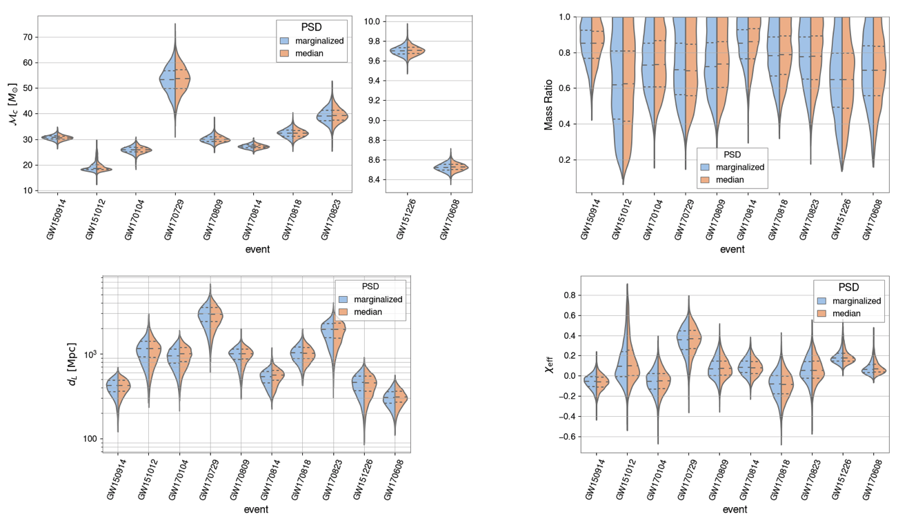
Figure 1: Violin plots showing the probability density for the PSD-marginalized posterior samples (blue) compared to the posterior samples obtained using the median PSD (orange) for the chirp mass, mass ratio, luminosity distance, and effective spin for each of the BBH detections. The horizontal lines represent the median (dashed) and $1\sigma$ confidence intervals (dotted) for each event.

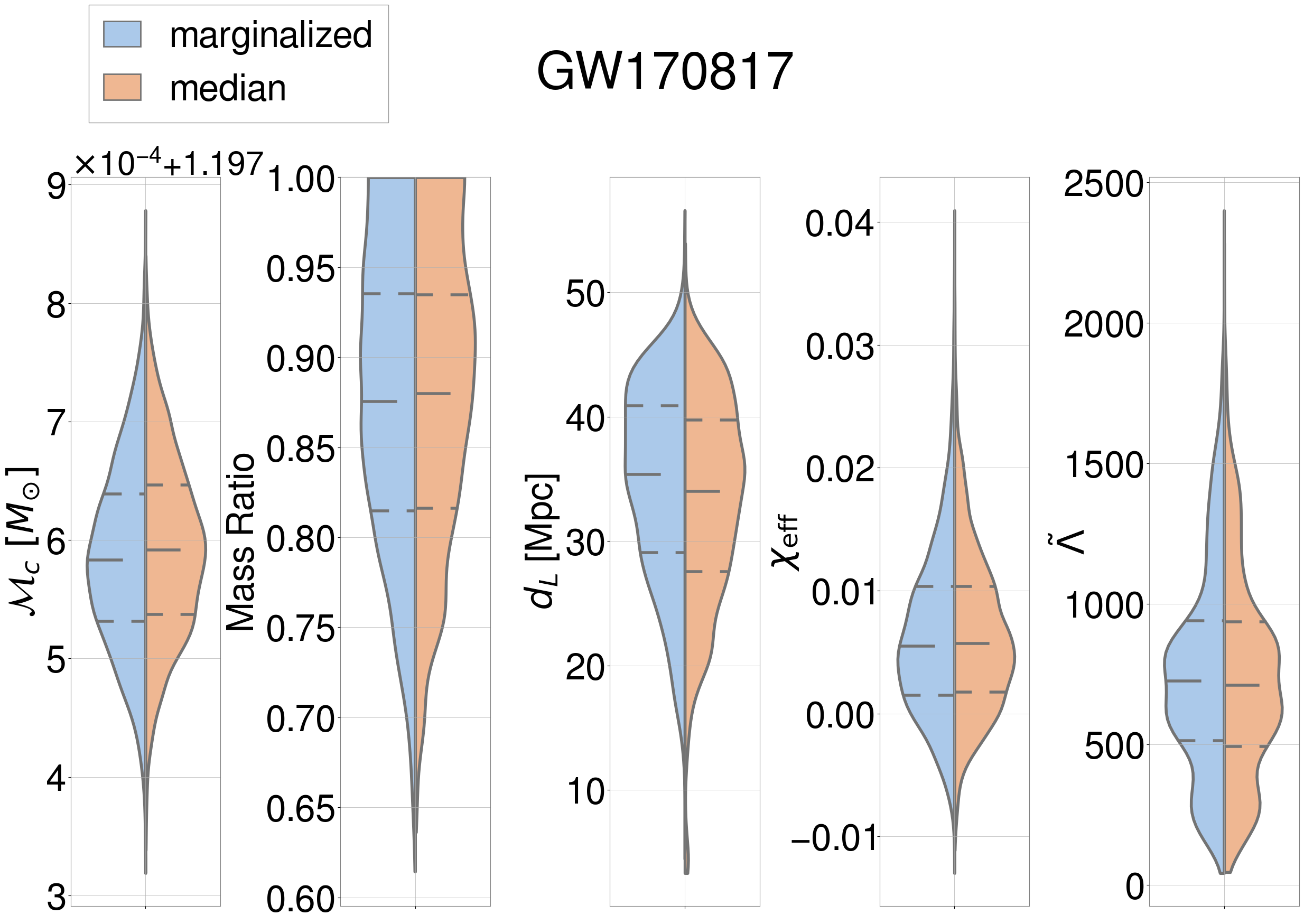
Figure 2: Violin plots showing the probability density for the PSD-marginalized posterior samples (blue) compared to the posterior samples obtained using the median PSD (orange) for the chirp mass, mass ratio, luminosity distance, effective spin, and mass-weighted average tidal deformability for the BNS, GW170817. The horizontal lines represent the median (dashed) and $1\sigma$ confidence intervals (dotted) for each parameter.

To quantify this effect, we show the difference in the width of the 90% and 50% confidence intervals between the PSD-marginalized and median PSD posteriors in Figs. 5 and 6 respectively for each event as a function of the network matched filter signal-to-noise ratio (SNR) calculated at the maximum likelihood point. The network SNR is obtained by adding the individual-detector SNRs in quadrature, where the matched filter SNR in a single detector is given byAllen et al. (2012):

$$\rho_{mf}=\frac{\langle d,h\rangle}{\sqrt{\langle h,h\rangle}},$$ (13)

for the inner product defined as:

$$\langle a,b\rangle=4\Re\int_{0}^{\infty}\frac{\tilde{a}^{*}(f)\tilde{b}(f)}{S_{n}(f)}\mathrm{d}f.$$ (14)

These results indicate that marginalizing over the uncertainty in the PSD produces posteriors that are wider than those obtained with the median PSD as a point estimate for about half of the events. The fractional change of the posterior width for both the 90% and 50% confidence intervals is of the order of a few percent, although a few larger excursions are observed for both confidence intervals. No significant trend is observed in the change in the confidence interval width as a function of the SNR, which indicates that the properties of the noise and the subsequent variation in the PSD are independent of the strength of the signal.

The largest deviation occurs in the 90% confidence interval of the chirp mass posterior of GW151012. This behavior can be explained by the variability in the Hanford PSD posterior at low frequencies shown in Fig. 3 that the median PSD cannot account for. This variability translates into significant posterior support for higher chirp masses for some of the individual PSD posterior samples, as shown in Fig. 4. This effect is minimized when averaging over the full PSD posterior, but not for the run with the median PSD alone, which also has increased support for higher chirp masses. Because the posterior obtained with the median PSD has wider tails, it has a correspondingly wider 90% confidence interval without affecting the 50% confidence interval, indicating good agreement between the two results for the bulk of their posterior distributions.

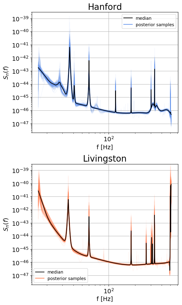
Figure 3: The 200 analyzed PSD posterior samples for the Hanford and Livingston LIGO detectors for GW151012 along with the median PSD in black

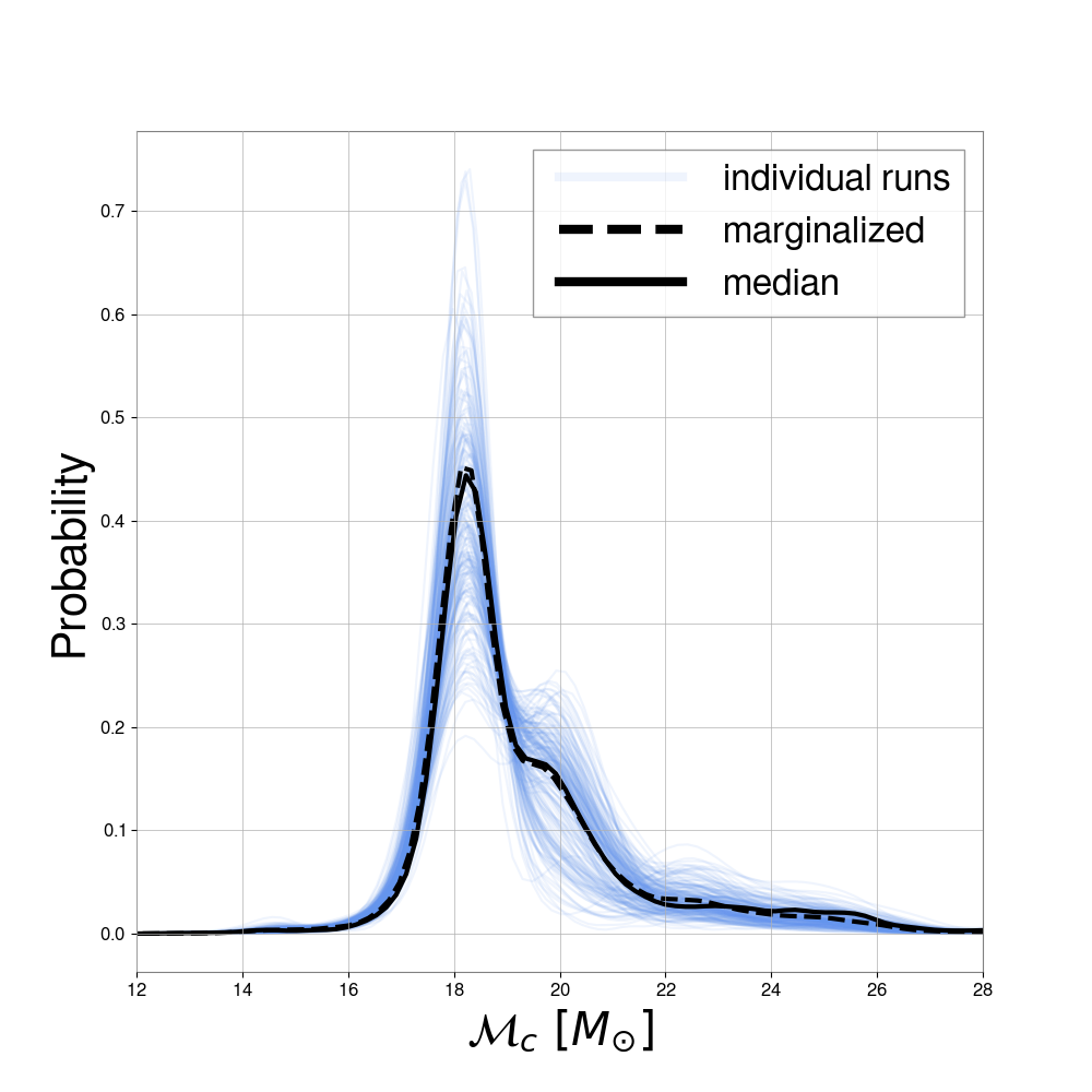
Figure 4: Kernel density estimate of the posterior on the detector-frame chirp mass for all 200 individual PSD posterior samples with the total PSD-marginalized posterior shown in the dotted black line and the posterior obtained with the median PSD in the solid black line for GW151012.

Table 2 shows the fractional change in the sky area $\Omega$, in square degrees, contained within the 50% and 90% confidence intervals between the PSD-marginalized and median PSD posteriors, $\Delta\Omega=(\Omega_{\mathrm{marg}}-\Omega_{\mathrm{med}})/\Omega_{\mathrm{marg}}$, as well as the absolute difference in the sky area contained in the 90% confidence interval. The change in the confidence intervals for the sky area exhibits similar variation to the other parameters shown in Figs. 5 and 6, on the order of $\sim 10\%$. The biggest deviations occur for the best-localized event, GW170817, although the total change is only a few square degrees for both confidence intervals.

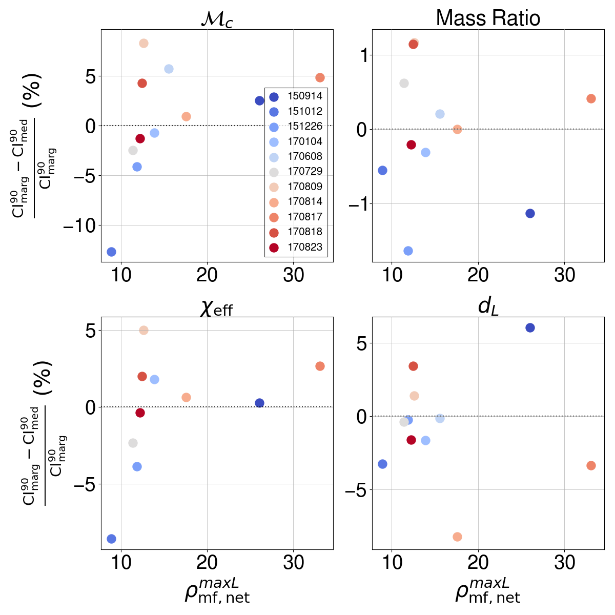
Figure 5: Normalized difference between the width of the 90% confidence interval of the PSD-marginalized and median PSD posteriors for chirp mass, mass ratio, effective spin, and luminosity distance for each event as a function of the maximum-likelihood network matched filter SNR calculated using the median PSD.

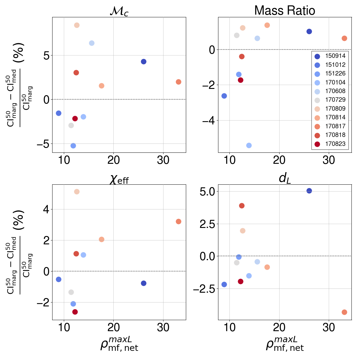
Figure 6: Normalized difference between the width of the 50% confidence interval of the PSD-marginalized and median PSD posteriors for chirp mass, mass ratio, effective spin, and luminosity distance for each event as a function of the maximum-likelihood network matched filter SNR calculated using the median PSD.

Event	$\Delta\Omega_{50}~{}(\%)$	$\Delta\Omega_{90}~{}(\%)$	$\Delta\Omega_{90}~{}(\mathrm{deg}^{2})$
GW150914	13.7	12.3	21
GW151012	1.5	-1.1	-20
GW151226	-9.6	-6.7	-93
GW170104	15.3	7.5	77
GW170608	-12.0	1.9	8
GW170729	19.0	10.4	136
GW170809	-12.1	2.9	9
GW170814	0	-18.6	-24
GW170817	28.6	25.9	7
GW170818	11.1	6.5	2
GW170823	2.9	-0.9	-14

Table 2: Fractional change in the 50% and 90% confidence intervals for the sky area in square degrees between the PSD-marginalized and median-PSD posteriors for each event, defined as $\Delta\Omega=(\Omega_{\mathrm{marg}}-\Omega_{\mathrm{med}})/\Omega_{\mathrm{marg}}$, and the absolute change in square degrees for the 90% confidence interval, which is $\Omega_{\mathrm{marg}}-\Omega_{\mathrm{med}}$.

In order to compare the posterior variations due to marginalizing over the PSD uncertainty to those expected due to statistical fluctuations, we use bootstrapping to generate different sets of samples from the median PSD posterior for different parameters and events. We find that on average the change in the width of the 90% confidence interval among the bootstrapped samples is of the order of $\sim 0.1\%$ across different events and parameters, about an order of magnitude smaller than the deviations we observe due to marginalizing over the PSD uncertainty.

IV Discussion

In this paper, we demonstrate a new method for marginalizing over the uncertainty in the noise power spectral density when performing gravitational wave parameter estimation for compact binary sources. We first obtain posterior samples for the PSD itself using the BayesWave software and then perform parameter estimation using 200 fair draws from the PSD posterior, combining the samples with equal weights to obtain the PSD-marginalized posterior. While no critical difference is observed in the posterior peak and shape for the binary parameters between the posteriors obtained using the median PSD as a point estimate and the PSD-marginalized posteriors, the posterior widths including the sky area vary on the order of a few percent, with the PSD-marginalized posterior being broader than that obtained using the median PSD for about half of the events. We do find more significant variation in the binary parameter posteriors obtained using individual PSD posterior samples for each gravitational-wave event, which can pick up secondary peaks or stronger support in the tail of the posterior, as was the case for GW151012. Based on these results, we conclude that the median PSD provides posteriors whose position and width are similar to those obtained when marginalizing over the PSD uncertainty to within a few percent for gravitational-wave signals of these SNRs observed in detectors with the current noise properties. The variations between the median and PSD-marginalized posteriors are an order of magnitude larger than those expected due to statistical fluctuations.

We close with a discussion of some caveats to our analysis. While we have shown that there is only minimal variation between the binary parameter posteriors obtained by marginalizing over the uncertainty in the PSD measurement and those obtained using the median PSD as a point estimate, we have not determined which of the two PSD models is preferred by the data. In our case, the two models we wish to compare are the “varied spline and Lorentzian model”, where the PSD is allowed to vary and is parameterized in terms of a broadband spline and a series of Lorentzians to fit narrowband features, and the “median PSD model”, where the PSD is fixed to the median of the full posterior computed with BayesWave. In both cases, the model also includes the presence of a CBC signal in the data, so we denote the varied spline and Lorentzian model as CBC+SL and the median PSD model as CBC+Me. This question of which model is statistically preferred is typically answered via Bayesian model selection and quantified using a Bayes factor between the two models being compared:

$$\mathrm{BF}^{\mathrm{CBC+SL}}_{\mathrm{CBC+Me}}=\frac{\mathcal{Z}^{\mathrm{CBC+SL}}}{\mathcal{Z}^{\mathrm{CBC+Me}}},$$ (15)

where the evidence, $\mathcal{Z}$, is defined as the normalization factor of the posterior obtained using a particular model. In addition to comparing the CBC+SL and CBC+Me models, obtaining the evidence under the CBC+SL model could also be used for comparing different variations of the CBC+SL model, for example precessing versus aligned compact binary component spins, the presence of higher order modes in the CBC waveform, or deviations from general relativity, which would all be represented as $\mathcal{Z}^{\mathrm{CBC+X+SL}}$.

Using the method described in Eq. 9, we obtain posterior samples for for the CBC+SL model but not an evidence:

$$\mathcal{Z}^{\mathrm{CBC+SL}}=p(d|\mathrm{CBC+SL}) =\int p(d|\theta,\mathrm{CBC+SL})$$ (16)

$$\times\pi(\theta|\mathrm{CBC+SL})\mathrm{d}\theta,$$

where $\pi(\theta|\mathrm{CBC+SL})$ is the prior defined in Eq. 7 where the explicit dependence on the $\mathrm{CBC+SL}$ model had previously been suppressed. $p(d|\mathrm{CBC+SL})$ is the likelihood of the data given the $\mathrm{CBC+SL}$ model, which we need to define in order to calculate the evidence above.

The evidence can be calculated during sampling if instead of marginalizing over the PSD uncertainty by combining the binary parameter posteriors obtained using different PSD posterior samples, the likelihood is modified to account for the PSD uncertainty, and this modified likelihood is used to estimate the PSD-marginalized binary parameters directly. The marginalized likelihood for the $\mathrm{CBC+SL}$ model is given by:

$$p(d|\theta,\mathrm{CBC+SL}) =\int p(d|\theta,S_{n},\mathrm{CBC+SL})$$ (17)

$$\times\pi(S_{n}|\mathrm{CBC+SL})\mathrm{d}S_{n}.$$

However, the likelihood $p(d|\theta,S_{n},\mathrm{CBC+SL})$ doesn’t depend on whether the PSD uncertainty is being included; it is equivalent to the likelihood for CBC signals defined in Eq. 3, so we drop the explicit dependence on $\mathrm{SL}$. Similarly, the prior on the PSD, $\pi(S_{n}|\mathrm{CBC+SL})$ doesn’t depend on the presence of a CBC signal, so we drop the dependence on $\mathrm{CBC}$:

$$p(d|\theta,\mathrm{CBC+SL}) =\int p(d|\theta,S_{n},\mathrm{CBC})$$ (18)

$$\times\pi(S_{n}|\mathrm{SL})\mathrm{d}S_{n}.$$

The prior on the PSD under the varied spline and Lorentzian model is the prior used by BayesWave, which is actually a complicated function of the spline and Lorentzian parameters and cannot be straightforwardly expressed in terms of $S_{n}$ directly. Unfortunately, it also cannot be extracted from the BayesWave sampler products. Since BayesWave must be run in the configuration where it also models the non-Gaussian data component from the astrophysical CBC signal in order to obtain an unbiased estimate of the PSD, the prior that can be constructed from the sampler products is a joint prior on the spline and Lorentzian parameters and the wavelet parameters used to model the non-Gaussian component. Thus, the marginalized likelihood in Eq.18 cannot be obtained using the two-step system we have employed in the rest of the analysis where the PSD is estimated first, separately from the estimation of the binary parameters. One possible way to obtain the evidence for the CBC+SL model would be to simultaneously estimate both the binary parameters and the PSD using the spline and Lorentzian parameterization.

We note that the likelihood under the CBC+Me model can be recovered from the form of the likelihood in Eq. 18 by substituting a Dirac delta for the prior on $S_{n}$:

$$\pi(S_{n}|\mathrm{SL})\rightarrow{}\pi(S_{n}|\mathrm{Me})=\delta(S_{n}-S_{n,\mathrm{Me}}).$$ (19)

The evidence for this model is hence obtained during the sampling of the binary parameters using the median PSD.

While our method is embarrassingly parallel, so that each of the $N$ parameter estimation analyses with different PSDs can be launched simultaneously, using the modified likelihood above requires that the CBC signal likelihood in Eq. 3 is evaluated $N$ times in series for each binary parameter sample. This computation could in principle be accelerated through the use of likelihood reweighting Payne et al. (2019) or other parallel processing techniques such as graphical processing units (GPUs) Talbot et al. (2019), multiprocessing Smith et al. (2019), or the Message Passing Interface (MPI) Snir et al. (1998). Furthermore, our method still requires $N$ times the computational resources compared to using the median PSD as a point estimate. We have chosen $N$=200 somewhat arbitrarily, balancing the computational cost against the number of samples needed to adequately represent the complete PSD posterior. We note, however, that producing the 200 draws from the PSD posterior comes at no extra computational cost compared to the production of the median PSD, so it would be possible to inspect the variability of the PSD posterior before starting the follow-up parameter estimation with each posterior draw. While we did find in the case of GW151012 that increased variability in the PSD posterior led to a larger change in the width of the binary parameter posteriors, there were also changes on the order of $\sim 5\%$ for events whose PSD posteriors seemed “smooth” like for the mass ratio of GW170104. We leave the systematic determination of the optimal $N$ to future work, along with the investigation of the applicability of the likelihood reweighting method to marginalization over PSD uncertainty.

We emphasize that while BayesWave can account for the presence of non-Gaussian “glitches” in the data such that they do not affect the inference of the PSD parameters, it still assumes that the noise is stationary and Gaussian over the duration of the analysis segment. Thus, the method we have described here does not include marginalizing over PSD uncertainty due to the variation of the noise properties over time. This should not have a significant effect for short signals like BBHs, but can be more pronounced for BNS signals requiring longer analysis segments Chatziioannou et al. (2019); Zackay et al. (2019).

Appendix A PSD Posteriors

In Figs. 7-9, we present the posteriors for the PSDs for each detector, LIGO–Hanford and LIGO–Livingston as well as Virgo where such data were available, for each event as well as the resulting median PSD.

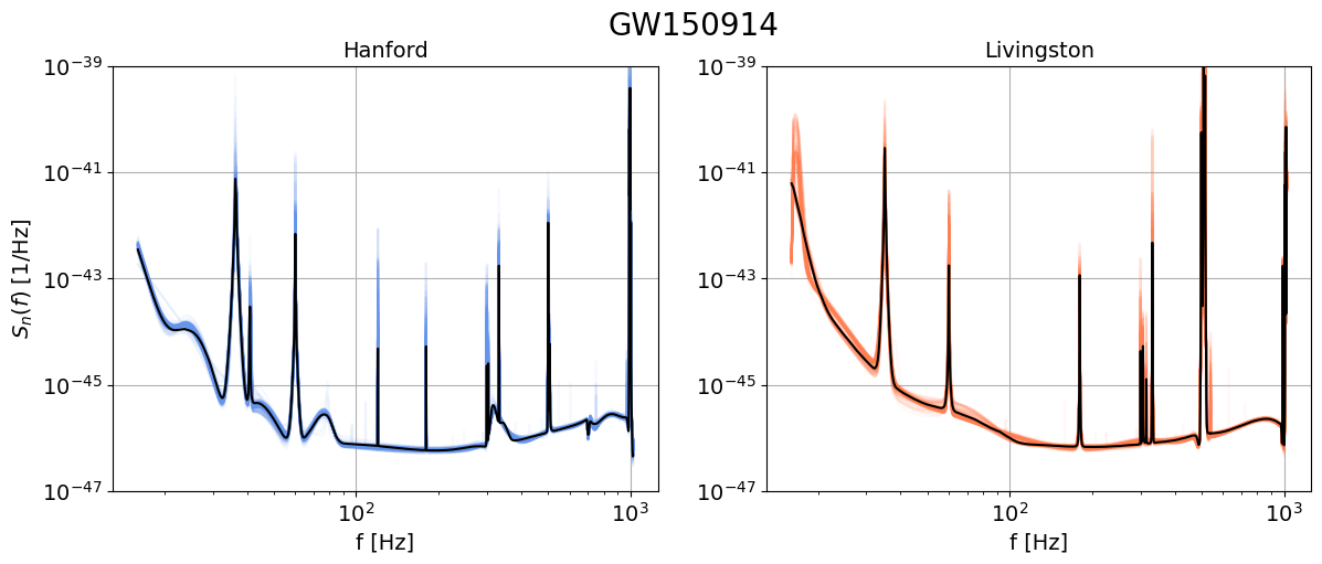
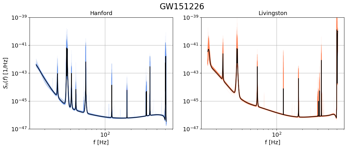
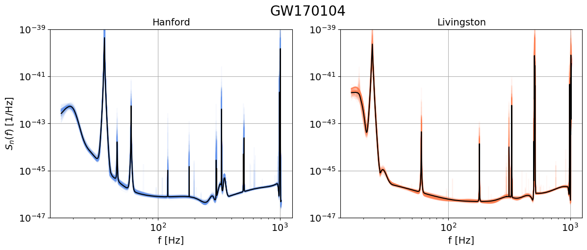
Figure 7: PSD posterior samples (colored lines) and the median PSD (black line) for each of the 11 events in GWTC-1. The PSDs start at 16 Hz, and the maximum frequency for each event is given in Table. 1.

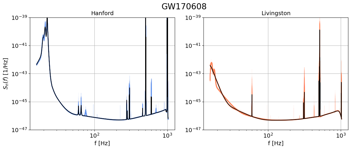
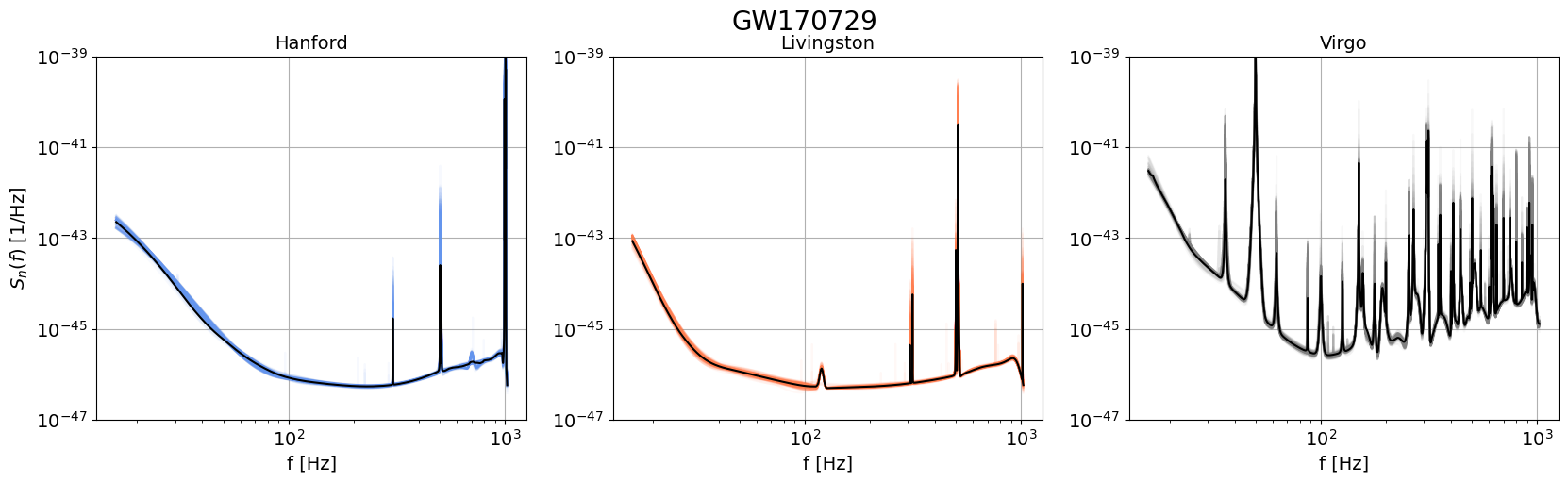
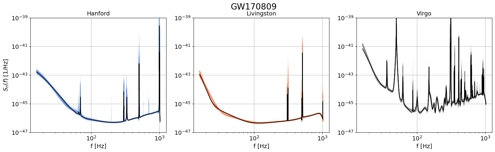
Figure 8: PSD posterior samples (colored lines) and the median PSD (black line) for each of the 11 events in GWTC-1. The PSDs start at 16 Hz, and the maximum frequency for each event is given in Table. 1.

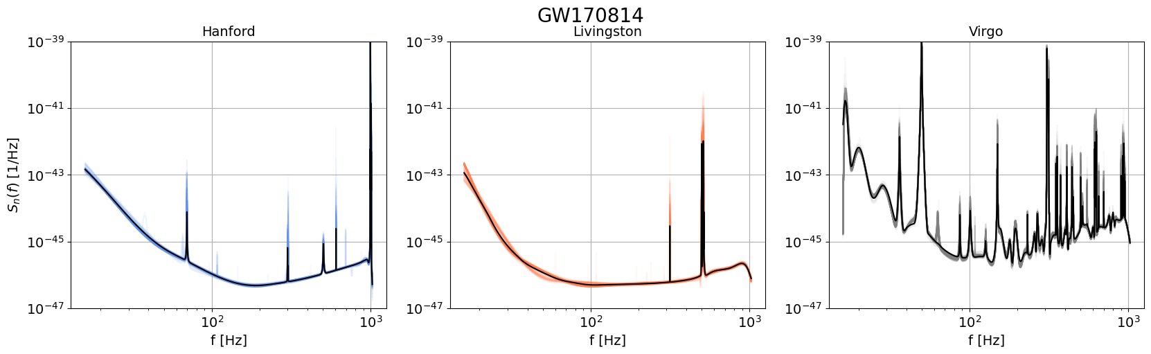
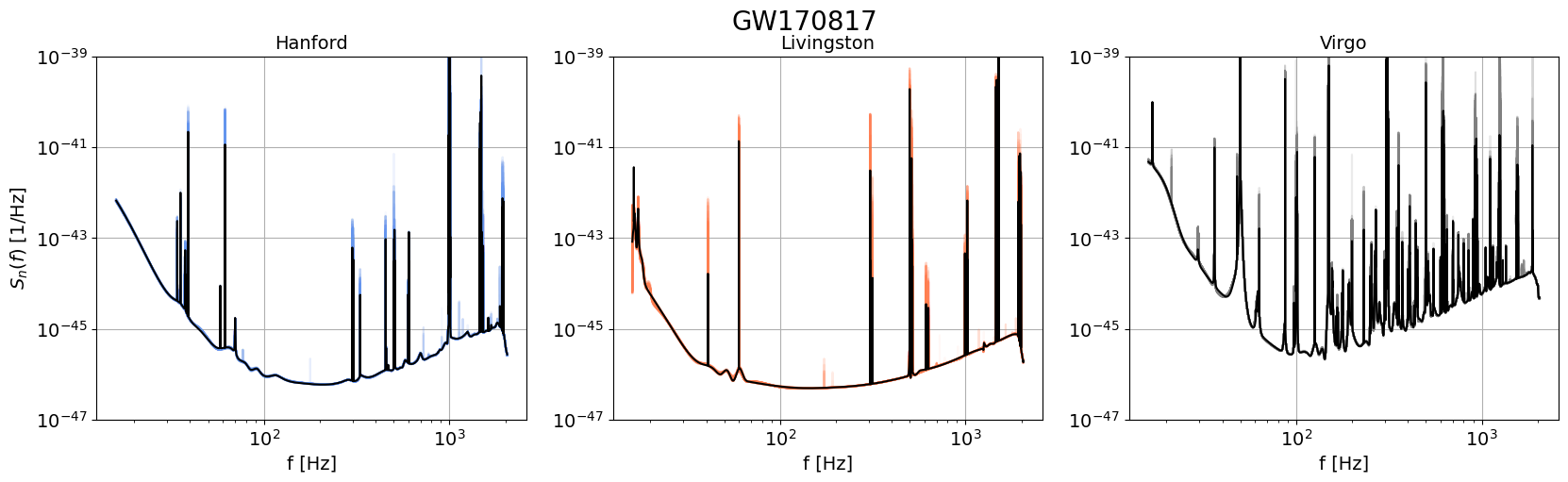
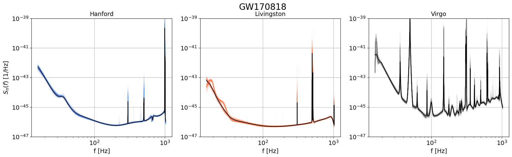
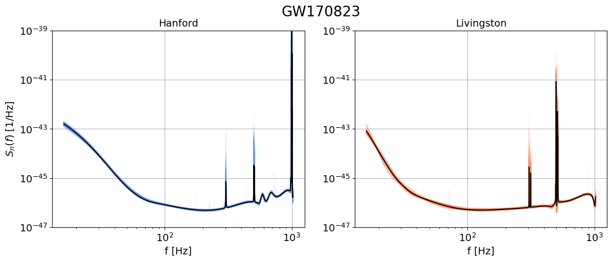
Figure 9: PSD posterior samples (colored lines) and the median PSD (black line) for each of the 11 events in GWTC-1. The PSDs start at 16 Hz, and the maximum frequency for each event is given in Table. 1.

References

- (1) https://git.ligo.org/sylvia.biscoveanu/psd_marginalized_event_samples.
- Aasi et al. (2015) J. Aasi et al. (LIGO Scientific), Class. Quant. Grav. 32, 074001 (2015), arXiv:1411.4547 [gr-qc] .
- Acernese et al. (2015) F. Acernese et al. (VIRGO), Class. Quant. Grav. 32, 024001 (2015), arXiv:1408.3978 [gr-qc] .
- Abbott et al. (2018a) B. P. Abbott et al. (KAGRA, LIGO Scientific, VIRGO), Living Rev. Rel. 21, 3 (2018a), arXiv:1304.0670 [gr-qc] .
- Messick et al. (2017) C. Messick et al., Phys. Rev. D95, 042001 (2017), arXiv:1604.04324 [astro-ph.IM] .
- Sachdev et al. (2019) S. Sachdev et al., ArXiV e-prints (2019), arXiv:1901.08580 [gr-qc] .
- Nitz et al. (2018) A. H. Nitz, T. Dal Canton, D. Davis, and S. Reyes, Phys. Rev. D98, 024050 (2018), arXiv:1805.11174 [gr-qc] .
- Usman et al. (2016) S. A. Usman et al., Class. Quant. Grav. 33, 215004 (2016), arXiv:1508.02357 [gr-qc] .
- Adams et al. (2016) T. Adams, D. Buskulic, V. Germain, G. M. Guidi, F. Marion, M. Montani, B. Mours, F. Piergiovanni, and G. Wang, Class. Quant. Grav. 33, 175012 (2016), arXiv:1512.02864 [gr-qc] .
- Chu (2017) Q. Chu, Low-latency detection and localization of gravitational waves from compact binary coalescences, Ph.D. thesis, The University of Western Australia (2017).
- Veitch et al. (2015) J. Veitch et al., Phys. Rev. D91, 042003 (2015), arXiv:1409.7215 [gr-qc] .
- Ashton et al. (2019) G. Ashton et al., Astrophys. J. Suppl. 241, 27 (2019), arXiv:1811.02042 [astro-ph.IM] .
- Huang et al. (2020) Y. Huang, C.-J. Haster, S. Vitale, A. Zimmerman, J. Roulet, T. Venumadhav, B. Zackay, L. Dai, and M. Zaldarriaga, ArXiV e-prints (2020), arXiv:2003.04513 [gr-qc] .
- Abbott et al. (2019a) B. P. Abbott et al. (LIGO Scientific, Virgo), Phys. Rev. X9, 031040 (2019a), arXiv:1811.12907 [astro-ph.HE] .
- Abbott et al. (2019b) B. Abbott et al. (LIGO Scientific, Virgo), Phys. Rev. D 100, 024017 (2019b), arXiv:1905.03457 [gr-qc] .
- Chatziioannou et al. (2019) K. Chatziioannou, C.-J. Haster, T. B. Littenberg, W. M. Farr, S. Ghonge, M. Millhouse, J. A. Clark, and N. Cornish, Phys. Rev. D100, 104004 (2019), arXiv:1907.06540 [gr-qc] .
- Abbott et al. (2018b) B. P. Abbott et al. (LIGO Scientific, Virgo), Class. Quant. Grav. 35, 065010 (2018b), arXiv:1710.02185 [gr-qc] .
- Aasi et al. (2013) J. Aasi et al. (LIGO Scientific, VIRGO), Phys. Rev. D88, 062001 (2013), arXiv:1304.1775 [gr-qc] .
- Zackay et al. (2019) B. Zackay, T. Venumadhav, J. Roulet, L. Dai, and M. Zaldarriaga, ArXiV e-prints (2019), arXiv:1908.05644 [astro-ph.IM] .
- Venumadhav et al. (2019) T. Venumadhav, B. Zackay, J. Roulet, L. Dai, and M. Zaldarriaga, Phys. Rev. D100, 023011 (2019), arXiv:1902.10341 [astro-ph.IM] .
- Mozzon et al. (2020) S. Mozzon, L. Nuttall, A. Lundgren, S. Kumar, A. Nitz, and T. Dent, (2020), arXiv:2002.09407 [astro-ph.IM] .
- Nitz et al. (2019) A. H. Nitz, T. Dent, G. S. Davies, S. Kumar, C. D. Capano, I. Harry, S. Mozzon, L. Nuttall, A. Lundgren, and M. Tápai, Astrophys. J. 891, 123 (2019), arXiv:1910.05331 [astro-ph.HE] .
- Nuttall et al. (2015) L. Nuttall et al., Class. Quant. Grav. 32, 245005 (2015), arXiv:1508.07316 [gr-qc] .
- Zevin et al. (2017) M. Zevin et al., Class. Quant. Grav. 34, 064003 (2017), arXiv:1611.04596 [gr-qc] .
- Abbott et al. (2016) B. P. Abbott et al. (LIGO Scientific, Virgo), Class. Quant. Grav. 33, 134001 (2016), arXiv:1602.03844 [gr-qc] .
- Pankow et al. (2018) C. Pankow et al., Phys. Rev. D98, 084016 (2018), arXiv:1808.03619 [gr-qc] .
- Welch (1967) P. Welch, IEEE Transactions on Audio and Electroacoustics 15, 70 (1967).
- Allen et al. (2012) B. Allen, W. G. Anderson, P. R. Brady, D. A. Brown, and J. D. E. Creighton, Phys. Rev. D85, 122006 (2012), arXiv:gr-qc/0509116 [gr-qc] .
- Littenberg and Cornish (2015) T. B. Littenberg and N. J. Cornish, Phys. Rev. D91, 084034 (2015), arXiv:1410.3852 [gr-qc] .
- Driggers et al. (2019) J. C. Driggers et al. (LIGO Scientific), Phys. Rev. D99, 042001 (2019), arXiv:1806.00532 [astro-ph.IM] .
- Davis et al. (2019) D. Davis, T. J. Massinger, A. P. Lundgren, J. C. Driggers, A. L. Urban, and L. K. Nuttall, Class. Quant. Grav. 36, 055011 (2019), arXiv:1809.05348 [astro-ph.IM] .
- Vajente et al. (2020) G. Vajente, Y. Huang, M. Isi, J. C. Driggers, J. S. Kissel, M. J. Szczepanczyk, and S. Vitale, Phys. Rev. D101, 042003 (2020), arXiv:1911.09083 [gr-qc] .
- Cornish and Littenberg (2015) N. J. Cornish and T. B. Littenberg, Class. Quant. Grav. 32, 135012 (2015), arXiv:1410.3835 [gr-qc] .
- Röver et al. (2011) C. Röver, R. Meyer, and N. Christensen, Class. Quant. Grav. 28, 015010 (2011), arXiv:0804.3853 [stat.ME] .
- Röver (2011) C. Röver, Phys. Rev. D84, 122004 (2011), arXiv:1109.0442 [physics.data-an] .
- Banagiri et al. (2020) S. Banagiri, M. W. Coughlin, J. Clark, P. D. Lasky, M. Bizouard, C. Talbot, E. Thrane, and V. Mandic, Mon. Not. Roy. Astron. Soc. 492, 4945 (2020), arXiv:1909.01934 [astro-ph.IM] .
- Smith and Thrane (2018) R. Smith and E. Thrane, Phys. Rev. X8, 021019 (2018), arXiv:1712.00688 [gr-qc] .
- Littenberg et al. (2013) T. B. Littenberg, M. Coughlin, B. Farr, and W. M. Farr, Phys. Rev. D88, 084044 (2013), arXiv:1307.8195 [astro-ph.IM] .
- Edwards et al. (2015) M. C. Edwards, R. Meyer, and N. Christensen, Phys. Rev. D 92, 064011 (2015), arXiv:1506.00185 [gr-qc] .
- Ashton and Khan (2020) G. Ashton and S. Khan, Phys. Rev. D 101, 064037 (2020), arXiv:1910.09138 [gr-qc] .
- Abbott et al. (2020) B. P. Abbott et al. (LIGO Scientific, Virgo), Class. Quant. Grav. 37, 055002 (2020), arXiv:1908.11170 [gr-qc] .
- Romano and Cornish (2017) J. D. Romano and N. J. Cornish, Living Rev. Rel. 20, 2 (2017), arXiv:1608.06889 [gr-qc] .
- Abbott et al. (2017a) B. P. Abbott et al. (LIGO Scientific Collaboration and Virgo Collaboration), Phys. Rev. Lett. 119, 161101 (2017a), arXiv:1710.05832 [gr-qc] .
- Bil (2019) “Bilby,” https://git.ligo.org/lscsoft/bilby (2019).
- Speagle (2020) J. S. Speagle, Mon. Not. Roy. Astron. Soc. 493, 3132 (2020), https://academic.oup.com/mnras/article-pdf/493/3/3132/32890730/staa278.pdf .
- Husa et al. (2016) S. Husa, S. Khan, M. Hannam, M. Pürrer, F. Ohme, X. Jiménez Forteza, and A. Bohé, Phys. Rev. D93, 044006 (2016), arXiv:1508.07250 [gr-qc] .
- Khan et al. (2016) S. Khan, S. Husa, M. Hannam, F. Ohme, M. Pürrer, X. Jiménez Forteza, and A. Bohé, Phys. Rev. D93, 044007 (2016), arXiv:1508.07253 [gr-qc] .
- Hannam et al. (2014) M. Hannam, P. Schmidt, A. Bohé, L. Haegel, S. Husa, F. Ohme, G. Pratten, and M. Pürrer, Phys. Rev. Lett. 113, 151101 (2014), arXiv:1308.3271 [gr-qc] .
- Dietrich et al. (2017) T. Dietrich, S. Bernuzzi, and W. Tichy, Phys. Rev. D96, 121501 (2017), arXiv:1706.02969 [gr-qc] .
- Dietrich et al. (2019) T. Dietrich et al., Phys. Rev. D99, 024029 (2019), arXiv:1804.02235 [gr-qc] .
- Smith et al. (2016) R. Smith, S. E. Field, K. Blackburn, C.-J. Haster, M. Pürrer, V. Raymond, and P. Schmidt, Phys. Rev. D94, 044031 (2016), arXiv:1604.08253 [gr-qc] .
- Burgay et al. (2003) M. Burgay et al., Nature 426, 531 (2003), arXiv:astro-ph/0312071 [astro-ph] .
- Abbott et al. (2017b) B. P. Abbott et al. (LIGO Scientific, Virgo), Astrophys. J. 851, L35 (2017b), arXiv:1711.05578 [astro-ph.HE] .
- Campanelli et al. (2006) M. Campanelli, C. O. Lousto, and Y. Zlochower, Phys. Rev. D74, 041501 (2006), arXiv:gr-qc/0604012 [gr-qc] .
- Racine (2008) É. Racine, Phys. Rev. D78, 044021 (2008), arXiv:0803.1820 [gr-qc] .
- Vitale et al. (2017) S. Vitale, R. Lynch, V. Raymond, R. Sturani, J. Veitch, and P. Graff, Phys. Rev. D95, 064053 (2017), arXiv:1611.01122 [gr-qc] .
- Ng et al. (2018) K. K. Y. Ng, S. Vitale, A. Zimmerman, K. Chatziioannou, D. Gerosa, and C.-J. Haster, Phys. Rev. D98, 083007 (2018), arXiv:1805.03046 [gr-qc] .
- Flanagan and Hinderer (2008) E. E. Flanagan and T. Hinderer, Phys. Rev. D77, 021502 (2008), arXiv:0709.1915 [astro-ph] .
- Favata (2014) M. Favata, Phys. Rev. Lett. 112, 101101 (2014), arXiv:1310.8288 [gr-qc] .
- Payne et al. (2019) E. Payne, C. Talbot, and E. Thrane, Phys. Rev. D100, 123017 (2019), arXiv:1905.05477 [astro-ph.IM] .
- Talbot et al. (2019) C. Talbot, R. Smith, E. Thrane, and G. B. Poole, Phys. Rev. D 100, 043030 (2019), arXiv:1904.02863 [astro-ph.IM] .
- Smith et al. (2019) R. Smith, G. Ashton, A. Vajpeyi, and C. Talbot, (2019), arXiv:1909.11873 [gr-qc] .
- Snir et al. (1998) M. Snir, S. Otto, S. Huss-Lederman, D. Walker, and J. Dongarra, MPI-The Complete Reference, Volume 1: The MPI Core, 2nd ed. (MIT Press, Cambridge, MA, USA, 1998).