Ising model with variable spin/agent strengths

Abstract

We introduce varying spin strengths to the Ising model, a central pillar of statistical physics. With inhomogeneous physical systems in mind, but also anticipating interdisciplinary applications, we present the model on network structures of varying degrees of complexity. This allows us explore the interplay of two types of randomness: individual strengths of spins or agents and collective connectivity between them. We solve the model for the generic case of power-law spin strength and find that, with a self-averaging free energy, it has a rich phase diagram with new universality classes. Indeed, the degree of complexity added by quenched variable spins is on a par to that added by endowing simple networks with increasingly realistic geometries. The model is suitable for investigating emergent phenomena in many-body systems in contexts where non-identicality of spins or agents plays an essential role and for exporting statistical physics concepts beyond physics.

• June 6, 2020

It is difficult to overestimate the importance of the Ising model (IM) in physics and beyond. It was invented 100 years ago by W. Lenz [1] and solved in one dimension with nearest-neighbour interactions by E. Ising [2]. It draws on works of R. Kirwan and W. Weber [3, 4] who proposed that vanishing magnetization of macroscopic para- and ferromagnetic bodies originates from random disordering of identical elementary magnets (spins) at microscopic levels. While their ideas also explained magnetic saturation in strong external fields, they failed to explain gradual response to weak ones. E.A. Ewing [5] introduced interactions to mend this shortcoming and P. Weiss [6] used the idea in the mean-field approximation. The IM itself sits between the Kirwan-Weber non-interacting picture and the Curie-Weiss maximally interacting one and manifests spontaneous spin alignment as well. Yet it is its simplicity, coupled with the phenomenon of universality, that lies behind its applicability to many real-world many-body phenomena in physics and beyond [7].

More elaborate models describe specific physical phenomena with greater precision, using greater levels of sophistication either in spin variables themselves or interactions among them. For the former case, the simple polarity, wherein spins have two possible states, is maintained in the continuous spin Ising model [8, 9]. This is relaxed in the Potts model while maintaining spin discreetness [10, 11] and the $m$-vector model goes further by introducing vector variables $\vec{\sigma}_{i}$ [12, 13]. Besides loosening Ising constraints on spins, they can be relaxed for interactions as well and simple extensions include next-nearest neighbour interactions, equivalent neighbours [14] or probabilistic long-range interactions [15], disorder and frustrations [16].

These variants deliver new universality classes, and, while associated models have been successful in their respective contexts, they rest on the same concept of interacting entities being identical. But not all particles are identical — they may have different inhomogeneities in internal degrees of freedom manifestating, e.g., different magnetic moments. None of the above models deal with this feature.

The IM brings physics beyond its traditional realms too. E.g., it models phenomena as diverse as cancer cells’ response to chemotherapy [17]; yield patterns in trees [18]; and advertising in duopoly markets [19]. Although each of these involves interactions between entities that are not spins, the IM is well placed to describe their collective properties. The importance of interactions in systems beyond physics is now well understood in society at large, as are consequences of not understanding this [21, 22]. Still, a protest often encountered when seeking to export statistical concepts is “people are not atoms” [24]. The term “agent” was introduced to reflect this linguistically but it does automatically de-binarise the interacting entities. Assurances such as “it is the law of big numbers which allows the application of statistical physics methods” [24] are often not understood, welcomed or accepted. Addressing these issues (the individuality of agents as well as the role of interactions) becomes important if we are to communicate physics to interdisciplinary colleagues or authorities; not all cells, trees or bankers are the same and there are different degrees of contagiousness among infected agents.

This suggest a new variant to the IM which, besides accounting for particle peculiarities, addresses non-identical agents. We introduce the model on network topologies for reasons applicable to both scenarios. In physics, there are nanosystems with topologies more akin to networks than lattices [25]. Varying spin strength in such systems may serve to model polydispersity in elementary magnetic moments [26]. Furthermore, perfect lattice structures are not common beyond physics and never encountered in sociophysics. Another example may be taken from neuroscience; in their recent review, Lynn and Bassett invite “creative effort” to “tackle some of the most pressing questions surrounding the inner workings of the mind” [27]. It is well known that cognition rests on heterogeneous connectivity structures in the brain and that neural communication strongly relies on a complex interplay between its network geometry and topology [28]. Introduction of variability to nodal strengths may likewise contribute to network modeling [29], accounting for differences in how nodes are defined as collections of brain tissue [30]. In particular, as an interacting unit in a brain network, the strength of a node may reflect its internal structure on a hierarchical level. A node may itself be composed of smaller nodes [31] or the changes in node strength may correspond to changes in node functionality over a span of time [32].

Here, we suggest and exactly solve an IM with variable spins/agents on networks of different degrees of complexity. Competition between individual agent strengths and collective connectivity generates a rich phase diagram suitable for the analysis of new universal emergent phenomena in many-agent systems [33].

Methods and Results

In the presence of a homogeneous field $H$, the Hamiltonian of the IM reads:

$${\cal H}=-\sum_{i<j}J_{ij}\sigma_{i}\sigma_{j}-H\sum_{i}\sigma_{i}\,,$$ (1)

For the standard version spins $\sigma_{i}$ take values $\pm 1$, $i=1\dots N$ and coupling $J_{ij}$ is $1$ for the nearest neighbour sites and $0$ otherwise. In sociophysics individuals are represented as nodes with binary spins representing different social states. This limitation is precisely because of the duality of spins in the generic IM. It may well be convincing for “for” or “against” options in referendums [23] but not all societal activities are binary and our model introduces gradation for individual node features.

We endow the spins $\sigma_{i}$ with “strengths” which vary from site to site through a random variable $|\sigma_{i}|\equiv\mathcal{S}_{i}$ drawn from probability distribution function $q(\mathcal{S}_{i})$. We chose a power-law decay:

$$q(\mathcal{S})=c_{\mu}\mathcal{S}^{-\mu},\hskip 28.45274pt\mathcal{S}_{\rm min}\leq\mathcal{S}\leq\mathcal{S}_{\rm max}\,,$$ (2)

where $c_{\mu}$ is a normalization constant, with $\mu>2$ ensuring finite mean strength $\overline{\mathcal{S}}$ when $\mathcal{S}_{\rm max}\to\infty$. The spin length being quenched random variable, a proper definition of thermodynamic functions involves configurational averaging besides the usual Gibbs averaging [34].

There are several obvious motivations for choosing a power-law form in the first instance. We don’t expect to encounter physical phenomena with spin strengths distributed precisely in this manner, but it is an established tradition in physics to take idealised models to investigate the fundamentals of a concept. Indeed Lenz and Ising applied this strategy when introducing the model in the first place. To take examples beyond physics, variable agent strength can be used to represent degrees of contagiousness in pandemics [20] or opinion in social systems.

Because of the interactive nature of the IM, these strengths impact on nodes with which a given node interacts — the greater the value of $\mathcal{S}_{i}$ the more contagious or persuasive node $i$ is. This new element is closer to real social networks and more likely to be accepted beyond physics [35]. Thus the introduction of variable spins to an established model opens new avenues to physics, interdisciplinarity and communication of same. As we shall see, these deliver very rich critical behavior and an onset of new accompanying phenomena which are of fundamental interest in their own right.

Since we are exploring new avenues, we consider three graph architectures which permit exact solutions: the complete graph, the Erdös-Rényi graph and scale-free networks. As in the Weiss model, every nodal pair $\{i,j\}$, is linked in the first case. The probability of connectedness is also the same for every nodal pair $p=p_{i,j}=c<1$ in the second case but it differs in that not every pair is linked. For the third case, the node degree distribution is governed by a power-law decay [36, 37]:

$$p(K)=c_{\lambda}K^{-\lambda},\hskip 28.45274ptK_{\rm min}\leq K\leq K_{\rm max}\,,$$ (3)

for constant $c_{\lambda}$ and $\lambda>2$. The adjacency matrix for an annealed random graph is [38, 39, 40]:

$$J_{ij}=\left\{\begin{array}[]{ccc}1,&\hskip 5.0ptp_{ij}\,,\\ 0,&\hskip 5.0pt1-p_{ij}\,,\end{array}\right.$$ (6)

where $p_{ij}$ is the edge probability  any pair $i$ and $j$. For $N$ nodes, one assigns a random degree $k_{i}$ to each, taken from the distribution

$$p_{ij}=\frac{k_{i}k_{j}}{N\overline{k}}+O(1/N^{2})\,,$$ (7)

with $\overline{k}=\frac{1}{N}\sum_{l}k_{l}$. The expected value of the node degree is $\mathbb{E}K_{i}=\sum_{j}p_{ij}=k_{i}$ and its distribution is given by $p(K)$ [39, 40]. The limiting cases $p_{ij}=1$ and $p_{ij}=c$ recover the complete and Erdös-Rényi random graph respectively.

Boltzmann averaging for the partition function is bond and spin-strength $\{\mathcal{S}\}$ configuration dependent. For annealed networks, averaging over links

$$\langle(\dots)\rangle_{\{J\}}=\prod_{i<j}\Big{[}(\dots)_{J_{ij}=1}p_{ij}+(\dots)_{J_{ij}=0}(1-p_{ij})\Big{]}\,$$ (8)

delivers equilibrium and is applied to the partition function vis.:

$$\langle{\cal Z}(\{J\},\{\mathcal{S}\})\rangle_{\{J\}}={\cal Z}(\{k\},\{\mathcal{S}\})\,.$$ (9)

The corresponding quenched free energy $f(\{k\},\{\mathcal{S}\})$ depends on the fixed random variables $\{k_{1},k_{2},\dots k_{N}\}\equiv\{k\}$ and $\{\mathcal{S}_{1},\mathcal{S}_{2},\dots\mathcal{S}_{N}\}\equiv\{\mathcal{S}\}$, These sequences are taken as fixed, quenched ones, so the free energy $f$ is obtained by averaging over them [34]. As we show below, the corresponding partition function, and thermodynamic functions are self-averaging; they do not depend on a particular choice of $\{k\}$ and $\{\mathcal{S}\}$.

Since the spin product in (1) can attain only two values, we use the equality

$$\phi(A\epsilon)=\frac{1}{2}[\phi(A)+\phi(-A)]+\frac{\epsilon}{2}[\phi(A)-\phi(-A)],\,\epsilon=\pm 1,$$

to get for the configuration-dependent partition function:

$${\cal Z}(\{k\},\{\mathcal{S}\})=\prod_{i<j}c_{ij}{\rm Sp}_{\sigma}\Big{(}e^{\sum_{i<j}d_{ij}\sigma_{i}\sigma_{j}+\beta H\sum_{i}\mathcal{S}_{i}\sigma_{i}}\Big{)}\ ,$$ (10)

$$c_{ij}=\sqrt{a_{ij}^{2}-b_{ij}^{2}},\,d_{ij}=\ln\frac{a_{ij}+b_{ij}}{a_{ij}-b_{ij}}\,.$$ (11)

Here, $\beta=T^{-1}$ is the inverse temperature, the trace is taken over all spins and we keep $\sigma_{i}=\pm 1$ representing each spin value as $\sigma_{i}\mathcal{S}_{i}$. The coefficients (11) implicitly depend on $p_{ij}$ and $\mathcal{S}_{i}$ via

$$a_{ij}=1-p_{ij}+p_{ij}\cosh(\beta J\mathcal{S}_{i}\mathcal{S}_{j}),\,b_{ij}=p_{ij}\sinh(\beta J\mathcal{S}_{i}\mathcal{S}_{j}).$$ (12)

The complete graph has $p_{ij}=1$, from which $c_{ij}=1$, $d_{ij}=2\beta\mathcal{S}_{i}\mathcal{S}_{j}$, and averaging over spins gives:

$${\cal Z}(\{\mathcal{S}\})=\int_{0}^{+\infty}e^{\frac{-x^{2}T}{2}}\Big{[}e^{I^{+}_{\mu}(\frac{x}{\sqrt{N}})}+e^{I^{-}_{\mu}(\frac{x}{\sqrt{N}})}\Big{]}dx\,,$$ (13)

having used (2) with $\mathcal{S}_{\rm max}\to\infty$. We obtain for small magnetic fields

$$I^{\pm}_{\mu}(\varepsilon)=N\Big{[}c_{\mu}\varepsilon^{\mu-1}I_{\mu}(\varepsilon)\pm\frac{\overline{\mathcal{S}^{2}}}{T}\varepsilon H\Big{]},$$ (14)

with

$$I_{\mu}(\varepsilon)=\int_{\varepsilon}^{\infty}dz\,\frac{1}{z^{\mu}}\ln\cosh z,$$ (15)

and $\varepsilon=\frac{x}{\sqrt{N}}$. In (13) and in all counterpart integral representations below, we omit irrelevant prefactors and numerical coefficients of associated response functions are presented elsewhere [41].

	$\alpha$	$\alpha_{c}$	$\gamma$	$\gamma_{c}$	$\beta$	$\delta$
Line 4 ($\lambda=\mu$)	$\frac{\lambda-5}{\lambda-3}$	$\frac{\lambda-5}{\lambda-2}$	1	$\frac{\lambda-3}{\lambda-2}$	$\frac{1}{\lambda-3}$	$\lambda-2$
Region III	$\frac{\lambda-5}{\lambda-3}$	$\frac{\lambda-5}{\lambda-2}$	1	$\frac{\lambda-3}{\lambda-2}$	$\frac{1}{\lambda-3}$	$\lambda-2$
Region IV	$\frac{\mu-5}{\mu-3}$	$\frac{\mu-5}{\mu-2}$	1	$\frac{\mu-3}{\mu-2}$	$\frac{1}{\mu-3}$	$\mu-2$
Region V, Lines 5,6, Point B	0	0	1	2/3	1/2	3

Table 1: Critical indices governing temperature and field dependencies of the specific heat, susceptibility, and order parameter in different parts of the phase diagram of Fig. 1.

	$\hat{\alpha}$	$\hat{\alpha_{c}}$	$\hat{\gamma}$	$\hat{\gamma_{c}}$	$\hat{\beta}$	$\hat{\delta}$
Line 4 ($\lambda=\mu$)	$-\frac{3}{\lambda-2}$	$-\frac{3}{\lambda-2}$	0	$-\frac{\lambda-3}{2(\lambda-2)}$	$-\frac{1}{\lambda-3}$	$-\frac{1}{\lambda-2}$
Point B	$-2$	$-2$	$0$	$-2/3$	$-1$	$-2/3$
Lines 5, 6	$-1$	$-1$	$0$	$-1/3$	$-1/2$	$-1/3$

Table 2: Logarithmic-correction exponents in different regions of Fig. 1. Exponents along line 4 ($\mu=\lambda$) and at point B represent new universality classes.

The partition function (13) is independent of $\{k\},\{\mathcal{S}\}$; for the random configuration $\{k\}$ this is obvious since $p_{ij}=1$ and for the random spin strength configuration $\{\mathcal{S}\}$ it is due to self-averaging. This is a generic feature of the model as we shall see below. With the asymptotic behavior of $I_{\mu}(\varepsilon)$ (15) to hand [42, 43, 41] one evaluates (13) in the thermodynamic limit $N\to\infty$ and obtains for the free energy per spin:

$$\frac{f}{N}\sim\left\{\begin{array}[]{lll}&m^{2}+m^{\mu-1}-mH,&2<\mu<3\,,\\ &m^{2}+m^{2}\ln\frac{1}{m}-mH,&\mu=3\,,\\ &\tau m^{2}+m^{\mu-1}-mH,&3<\mu<5\,,\\ &\tau m^{2}+m^{4}\ln\frac{1}{m}-mH,&\mu=5\,,\\ &\tau m^{2}+m^{4}-mH,&\mu>5\,.\end{array}\right.$$ (16)

Here, $m$ is the order parameter and $\tau$ is the reduced temperature. A similar free energy describes the critical behavior of the standard IM ($\sigma_{i}=\pm 1$) on an annealed scale-free network, with decay exponent $\lambda$ in that case [40] playing the role of $\mu$ in the current one. The system is ordered at any finite temperature when $\mu\leq 3$ and has a second order phase transition when $\mu>3$. All universal characteristics of the transition are $\mu$-dependent when $3<\mu<5$ and the $\mu>5$ region is mean-field like. At $\mu=5$ logarithmic corrections feature [37, 38, 39, 40, 44], governed by exponents which adhere to the usual scaling relations [45]. These and leading exponents are listed in the third row of Table 1 and discussed in further detail in that context.

For Erdös-Rényi graphs one substitutes $p_{ij}=c$ into (11). This delivers a similar partition function (10) to that of the complete graph up to renormalized interaction so that critical behaviors of both models are essentially equivalent.

For annealed scale-free networks, with $p_{ij}$ given by (7), the thermodynamic limit $N\to\infty$ (i.e. with small $p_{ij}$) applied to (11) gives $d_{ij}\sim p_{ij}\beta J\mathcal{S}_{i}\mathcal{S}_{j}$. The Stratonovich-Hubbard transformation delivers the trace over spins in (10) and a partition function that has unary dependency on the random variables $f(k_{i}\mathcal{S}_{i})$. It is convenient to pass from the summation over nodes $i$ to summation over random variables $k_{i}$, $\mathcal{S}_{i}$

$$\sum_{i=1}^{N}f(k_{i}\mathcal{S}_{i})=N\sum_{k=k_{\rm min}}^{k_{\rm max}}\sum_{\mathcal{S}=\mathcal{S}_{\rm min}}^{\mathcal{S}_{\rm max}}p(k)q(\mathcal{S})f(k,\mathcal{S})\,.$$

Considering the variables $k$ and $\mathcal{S}$ as continuous and taking the thermodynamic limit $N\to\infty$, we put $k_{\rm max}=\mathcal{S}_{\rm max}\to\infty$ and we choose the lower bounds $k_{\rm min}=\mathcal{S}_{\rm min}=2$ [41]. It is straightforward to see that the partition function ${\cal Z}(\{\mathcal{S}\},\{k\})$ is independent of the random variables $k$ and $\mathcal{S}$ and is self-averaging. Indeed, when both distribution functions $p(k)$, $q(\mathcal{S})$ attain power-law forms (2), (3) we obtain

$${\cal Z}=\int_{0}^{+\infty}e^{\frac{-\overline{k}T}{2N}x^{2}}\Big{[}e^{I^{+}_{\lambda,\mu}(\sqrt{\frac{x}{N}})}+e^{I^{-}_{\lambda,\mu}(\sqrt{\frac{x}{N}})}\Big{]}\,dx\,,$$ (17)

and

$$I^{\pm}_{\lambda,\mu}(\varepsilon)=N\Big{[}c_{\lambda}c_{\mu}\Big{(}\frac{\varepsilon}{2}\Big{)}^{\lambda+\mu-2}I_{\lambda,\mu}(\varepsilon)\pm\frac{\overline{\mathcal{S}^{2}}\,\overline{k}}{4T}\varepsilon^{2}H\Big{]}$$ (18)

where

$$I_{\lambda,\mu}(\varepsilon)=\int_{\varepsilon}^{\infty}\int_{\varepsilon}^{\infty}\varphi(k,\mathcal{S})\,d\mathcal{S}dk\,$$ (19)

with

$$\varphi(k,\mathcal{S})=\frac{1}{k^{\lambda}\mathcal{S}^{\mu}}\ln\cosh\Big{(}k\mathcal{S}\Big{)},$$ (20)

and the lower integration bound $\varepsilon=2\sqrt{x/N}$ tends to zero, when $N\rightarrow\infty$.

As in the case of the model on the complete graph (15), the partition function (17) and hence the of the free energy is determined by the asymptotics of the integral (19) as $\varepsilon\to 0$. This is governed by the interplay of the decay exponents $\lambda$ and $\mu$. In particular, for the diagonal case $\lambda=\mu$ we get:

$$I_{\lambda,\lambda}(\varepsilon)=a_{\lambda}+b_{\lambda}\ln(\varepsilon)i_{\lambda}(\varepsilon)\,,$$ (21)

with

$$i_{\lambda}(\varepsilon)\simeq\left\{\begin{array}[]{lll}&O(\varepsilon^{2}),&2<\lambda<3\,,\\ &(\ln\varepsilon)^{2}/2+O(\varepsilon^{4}),&\lambda=3\,,\\ &{\frac{\varepsilon^{6-2\lambda}}{2(\lambda-3)^{2}}}+O(\varepsilon^{2}),&3<\lambda<5\,,\\ &\varepsilon^{-4}/8+(\ln\varepsilon)^{2}/6+O(\varepsilon^{2}),&\lambda=5\,,\\ &{\frac{\varepsilon^{6-2\lambda}}{2(\lambda-3)^{2}}}-{\frac{\varepsilon^{10-2\lambda}}{12(\lambda-5)^{2}}}+O(\varepsilon^{2}),&5<\lambda<7\,.\end{array}\right.$$ (27)

The constants in (21) can be readily evaluated and are presented elsewhere [41]. For the non-diagonal case $\mu\neq\lambda$, due to the symmetry $I_{\lambda,\mu}=I_{\mu,\lambda}$ it is enough to evaluate the integral for $\lambda>\mu$. With estimates available from [41], we apply the steepest descent method to get the exact solution for the partition function (17). The results that follow from the analysis of the free energy are summarized in Fig. 1 and  Tables 1, 2.

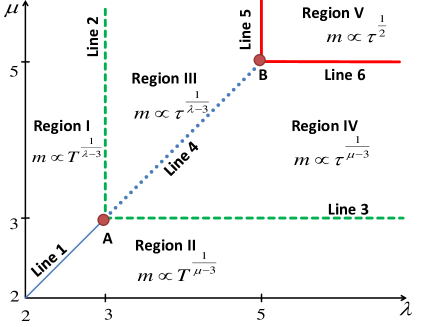
Figure 1: Phase diagram of the IM with power-law distributed spin strength (2) on an annealed scale free network with node degree distribution (3). See Tables 1, 2.

Fig. 1 presents the phase diagram of the model in the $\lambda-\mu$ plane. Behavior is controlled by the parameter with the smaller value. In Regions I and II, for which distributions are fat-tailed with $\lambda<3$ or $\mu<3$, the system remains ordered at any finite temperature $T$. There, the order parameter decays with $T$ as a power law, $m\sim T^{\frac{1}{\lambda-3}}$ or $m\sim T^{\frac{1}{\mu-3}}$ for $2<\lambda<3$ and $2<\mu<3$, correspondingly. Both asymptotics coincide along Line 1 in the figure.

The decay is exponential $m\sim Te^{-T}$ along Lines 2 and 3 where $\lambda=3$ or $\mu=3$ as well as at point A where they coincide. Second order phase transitions occur when both $\lambda,\mu>3$. In Region III where $3<\lambda<5$ ($\mu>\lambda$) the critical exponents are $\lambda$-dependent and in Region IV where $3<\mu<5$ ($\mu<\lambda$) they are $\mu$-dependent.

When $\lambda=5$ or $\mu=5$ logarithmic corrections to scaling appear. For example, the order parameter in Lines 4-6 behaves as $m\sim\tau^{\beta}|\ln\tau|^{-\hat{\beta}}.$ The values of the logarithmic correction exponents in Lines 5 and 6 coincide with those for the IM on a scale-free network [40, 44]. The additional richness of the phase diagram is characterised, for example, by new type of logarithmic corrections which emerge in Line 4 where $3<\lambda=\mu<5$ as well as Point B where $\lambda=\mu=5$. All of them obey the scaling relations for logarithmic corrections [45]. Critical exponents are summarized in Tables 1 and 2.

Thus introduction of variable spin or agent strengths to the IM on networks delivers rich new phase diagrams and universality classes relevant to circumstances wherein interacting spins and agents carry degrees of complexity over and above the binary features mostly considered in physics and often rejected in other disciplines. On the other hand, introducing random variables into the IM either in form of annealed network or random spin strength makes the interaction separable, as in Mattis [46] or Hopfield models [47] used in description of spin glasses.

The model with power-law decaying random strength distribution (2) on the complete graph has similar critical behavior to the standard IM on a scale-free network with random node degree distribution (3) with decay exponents $\mu$ and $\lambda$ playing equivalent roles. This suggests that the level of complexity introduced by allowing spin strengths to vary is on a par to the level of complexity introduced by allowing network architecture to vary; i.e., individual strength matter as much as connectivity.

When introduced to already rich annealed scale-free network the complexity level is magnified yet more. Besides self-averaging, it is governed by the concurrence of two parameters describing different phenomena arising from inherent interplay of two types of randomness. The full phase diagram of the model (Fig. 1) is symmetric under $\mu\leftrightarrow\lambda$ interchange, critical behavior governed by the smaller of the two parameters. Ordering, critical behaviour and logarithmic corrections all feature.

The IM itself taught us that interactions in physics play as important a role as spin properties, for without them we have no cooperative behavior or spontaneous magnetization. We have seen that spin strength and system architecture play similar counterbalancing roles and are tuned by the exponents $\mu$ and $\lambda$. In sociophysics terms they suggest duality between strength of individual opinions and societal cohesion. We hope that introduction of the former to the Ising model goes some way to addressing interdisciplinary objections that “people are not atoms” [24]. But we hope the variable-strength Ising model is suggestive of more than this too. Region V of the phase diagram has high values of $\mu$ and $\lambda$ which may be interpreted as representing populism and weak society. Regions I and II, on the other hand, represent empowerment of individuals and high social connectivity. Regions III and IV then represent the critical divide between these very different societies and suggests critical phenomena may play a role in further studies of the interplay between the individual and the collective.

References

- [1] Lenz W., Phys. Zeitschrift, 21 (1920) 613.
- [2] Ising E., Beitrag zur Theorie des Ferro- und Paramagnetismus (Doctoral dissertation, Hamburg, 1924) http://www.icmp.lviv.ua/ising/books.html; Ising E., Z. Physik, 31 (1925) 253.
- [3] Kirwan R., The Transactions of the Royal Irish Academy, 6 (1797) 177.
- [4] Weber W., Annalen der Physik, 87 (1852) 145.
- [5] Ewing E.A., Proc. Roy. Soc., 48 (1890) 342.
- [6] Weiss P., Comptes Rendus des Séances de l’Académie des Sciences, 143 (1906) 1136.
- [7] Ising T., Folk R., Kenna R., Berche B., and Holovatch Yu., Journ. Phys. Stud., 21 (2017) 3002.
- [8] van Beijeren H. and Sylvester G.S., J. Func. Analysis, 28 (1978) 145.
- [9] Bayong E. and Diep H. T., Phys. Rev. B, 59 (1999) 11919.
- [10] Potts R.B., Math. Proc. Cambridge Phil. Soc., 48 (1952) 106.
- [11] Wu F.-Y., Rev. Mod. Phys., 54 (1982) 235.
- [12] Stanley H.E., Phys. Rev. Lett., 20 (1968) 589.
- [13] Stanley H.E., Phase transitions and critical phenomena (Clarendon Press, Oxford) 1971.
- [14] Luijten E., Blöte H.W.J. and Binder K., Phys. Rev. E, 54 (1996) 4626.
- [15] Fisher M.E., Ma S.-K. and Nickel B. G., Phys. Rev. Lett., 29 (1972) 917.
- [16] See e.g. Mezard M., Parisi G. and Virasoro M., Spin Glass Theory and Beyond (World Scientific, Singapore) 1986; Dotsenko V., An Introduction to the Theory of Spin Glasses and Neural Networks (World Scientific, Singapore) 1994.
- [17] Arbabi Moghadam S., Rezania V., Tuszynski J.A., R. Soc. Open Sci., 7 (2020) 191578.
- [18] Noble A.E., Rosenstock T.S., Brown P.H., Machta J. and Hastings A., PNAS, 115 (2018) 1825.
- [19] Sznajd-Weron K. and Weron R., Physica A, 324 (2003) 437.
- [20] There is already a plethora of papers about Covid-19 on the arXiv. From the reaction of the academic community to the Chornobyl disaster this is likely to persist indefinitely. See Mryglod O., Holovatch Yu., Kenna R. and Berche B., Scientometrics, 106 (2016) 1151-1166.
-
[21]
Public request to take stronger measures of social distancing
across the UK with immediate effect, 14th March 2020
http://maths.qmul.ac.uk/~vnicosia/UK_scientists\_
statement\_on\_coronavirus\_measures.pdfΩ
- [22] Penser la pandémie du Covid-19 (2 et son annexe), 20 May 2020 http://www.sauvonsluniversite.fr/spip.php?article8714
- [23] Galam S., Sociophysics: A Physicists Modeling of Psycho - Political Phenomena (Springer-Verlag) 2012.
- [24] Stauffer D., J. Stat. Phys., 151 (2013) 9.
- [25] Tadić B., Malarz K. and Kułakowski K., Phys. Rev. Lett., 94 (2005) 137204.
- [26] Russier V., de Montferrand C., Lalatonne Y., and Motte L., J. Appl. Phys. 12 (2012) 073926.
- [27] Lynn C. W. and Bassett D. S., Nature Reviews Physics 1 (2019) 318.
- [28] Seguin C., van den Heuvel M. P. and Zalesky A., PNAS 115 (2018) 6297.
- [29] Betzel R. F. and Bassett D. S., J. R. Soc. Interface 14 (2017) 20170623.
- [30] Stanley M. L. et al., Frontiers in Computational Neuroscience 7 (2013) 169.
- [31] Park H.-J. and Friston K. Science 342 (2013) 1238411.
- [32] Bagarinao E. et al., Scientific Reports 9 (2019) 11352.
- [33] Holovatch Yu., Kenna R. and Thurner S., Eur. Journ. Phys., 38 (2017) 023002.
- [34] Brout R., Phys. Rev., 115 (1959) 824.
-
[35]
No more than 10% of world leaders have mathematical or scientific
backgrounds:
https://www.studyinternational.com/news/what-to-
study-if-you-want-to-be-a-politician-based-on-
current-world-leaderΩ
- [36] Newman M., Networks: An Introduction (Oxford University Press) 2010.
- [37] Dorogovtsev S. N., Goltsev A. V. and Mendes J.F.F., Rev. Mod. Phys., 80 (2008) 1275.
- [38] Lee S.H., Ha M., Jeong H., Noh J.D. and Park H., Phys. Rev. E, 80 (2009) 051127.
- [39] Bianconi G., Phys. Rev. E, 85 (2012) 061113.
- [40] Krasnytska M., Berche B., Holovatch Yu. and Kenna R., Europhys. Lett., 111 (2015) 60009; J. Phys. A, 49 (2016) 135001.
- [41] Krasnytska M., Berche B., Holovatch Yu. and Kenna R., in preparation.
- [42] Iglói F. and Turban L., Phys. Rev. E, 66 (2002) 036140.
- [43] Krasnytska M., Berche B., Holovatch Yu., Condens. Matter Phys., 16 (2013) 23602.
- [44] Leone M., Vzquez A., Vespignani A., and Zecchina R., Eur. Phys. J. B, 28 (2002) 191; Dorogovtsev S., Goltsev A.V. and Mendes J.F.F., Eur. Phys. J. B, 38 (2004) 177; von Ferber C., Folk R., Holovatch Yu., Kenna R. and Palchykov V., Phys. Rev. E, 83 (2011) 061114.
- [45] Kenna R., in Order, Disorder, and Criticality: Advanced Problems of Phase Transition Theory, Edited by Holovatch Yu., vol. 3 (World Scientific, Singapore) 2012, pp 1-46.
- [46] Mattis D.C., Phys. Lett. A, 56 (1976) 421; Bianconi G., Phys. Lett. A, 303 (2002) 166.
- [47] Pastur L.A. and Figotin A.L., Sov. J. Low Temp. Phys., 3(6) (1977) 378; Pastur L.A. and Figotin A.L., Theor. Math. Phys., 35 (1978) 403; Hopfield J.J., Proc. Natl. Acad. Sci. USA, 79 (1982) 2554.