Abstract

As a tractable approach, regularization is frequently adopted in sparse optimization. This gives rise to the regularized optimization, aiming at minimizing the $\ell_{0}$ norm or its continuous surrogates that characterize the sparsity. From the continuity of surrogates to the discreteness of $\ell_{0}$ norm, the most challenging model is the $\ell_{0}$-regularized optimization. To conquer this hardness, there is a vast body of work on developing numerically effective methods. However, most of them only enjoy that either the (sub)sequence converges to a stationary point from the deterministic optimization perspective or the distance between each iterate and any given sparse reference point is bounded by an error bound in the sense of probability. In this paper, we develop a Newton-type method for the $\ell_{0}$-regularized optimization and prove that the generated sequence converges to a stationary point globally and quadratically under the standard assumptions, theoretically explaining that our method is able to perform surprisingly well.

Keywords: $\ell_{0}$-regularized optimization, $\tau$-stationary point, Newton method, Global and quadratic convergence

Mathematical Subject Classification: 65K05$\cdot$ 90C46$\cdot$ 90C06$\cdot$ 90C27

1 Introduction

Over the last decade, sparsity has been thoroughly investigated due to its extensive applications ranging from compressed sensing [23, 15, 16], signal and image processing [25, 24, 17, 8], machine learning [48, 53] to neural networks [7, 33, 22] lately. Sparsity is frequently characterized by $\ell_{0}$ norm and its penalized problem is commonly phrased as $\ell_{0}$-regularized optimization, taking the form of

(1.1) $$\min_{{\rm x}\in\mathbb{R}^{n}}~{}~{}f({\rm x})+\lambda\|{\rm x}\|_{0},$$

where $f:\mathbb{R}^{n}\rightarrow\mathbb{R}$ is twice continuously differentiable and bounded from below, $\lambda>0$ is the penalty parameter and $\|{\rm x}\|_{0}$ is $\ell_{0}$ norm of ${\rm x}$, counting the number of non-zero elements of ${\rm x}$. Differing from the regularized optimization, another category of sparsity involved problems that have been well studied is the so-called sparsity constrained optimization:

(1.2) $$\min_{{\rm x}\in\mathbb{R}^{n}}~{}f({\rm x}),~{}~{}~{}{\rm s.t.}~{}\|{\rm x}\|_{0}\leq s,$$

where $s\leq n$ is a given positive integer. Based on the two optimizations, large numbers of state-of-the-art methods have been proposed in the last decade. In particular, many of them are designed for a special application, compressed sensing (CS), where the least squares are taken into account, namely

(1.3) $$f({\rm x}):=f_{cs}({\rm x})\equiv\|A{\rm x}-{\rm y}\|^{2}.$$

Here, $A\in\mathbb{R}^{m\times n}$ is the sensing matrix and ${\rm y}\in\mathbb{R}^{m}$ is the measurement.

1.1 Selective Literature Review

Since there is a vast body of work developing numerical methods to solve the (1.2) or (1.1), we present a brief overview of work that is able to clarify our motivations of this paper.

(a) Methods for (1.2) are known as greedy ones. For the case of CS, one can refer to orthogonal matching [40, 47, OMP], gradient pursuit [12, GP], compressive sample matching pursuit [38, CoSaMP], subspace pursuit [20, SP], normalized iterative hard-thresholding [14, NIHT], hard-thresholding pursuit [28, HTP] and accelerated iterative hard-thresholding [11, AIHT]. Methods for the general model (1.2) include the gradient support pursuit [2, GraSP], iterative hard-thresholding [4, IHT], Newton gradient pursuit [52, NTGP], conjugate gradient iterative hard-thresholding [10, CGIHT], gradient hard-thresholding pursuit [51, GraHTP], improved iterate hard-thresholding [39, IIHT] and Newton hard-thresholding pursuit [55, NHTP].

To derive the convergence results, most methods enjoy the theory that the distance between each iterate to any given reference (sparse) point is bounded by an error through statistic analysis. By contrast, methods like IHT, IIHT and NHTP have been proved to converge to a stationary point globally in the sense of the deterministic way. Moreover, if Newton directions are interpolated into some methods, for example, CoSaMP, SP, GraSP, NTGP and GraHTP, then their demonstrated empirical performances are extraordinary in terms of super-fast computational speed and high order of accuracy, but without deterministic theoretical guarantees for a long time. Until recently, authors in [55] first proved that their proposed NHTP has global and quadratic convergence properties, which unravel the reason why these methods behave exceptionally well.

(b) Methods for (1.1) aiming at addressing CS problem via the model (1.1) include iterative hard-thresholding algorithm [13, IHT], continuous exact $\ell_{0}$ penalty [44, CEL0], two methods: continuation single best replacement and $\ell_{0}$-regularization path descent in [45, CSBR, L0BD], forward-backward splitting [1, FBS], extrapolated proximal iterative hard-thresholding algorithm [3, EPIHT] and mixed integer optimization method [6, MIO], to name just a few. While for the general problem (1.1), one can see penalty decomposition [36, PD] where equality and inequality constraints are also considered, iterative hard-thresholding [35, see] where the box and convex cone are taken into account, proximal gradient method and coordinate-wise support optimality method [5, PG, CowS] where sparse solutions are sought from a symmetric set, random proximal alternating minimization method [41, RPA], active set Barzilar-Borwein [18, ABB] and a very recently smoothing proximal gradient method [9, SPG]. Note that these methods can be regarded as the first-order methods since they only benefit from the first-order information such as gradients or function values. Then second-order methods have attracted much attention lately, including primal dual active set [30, PDAS], primal dual active set with continuation [31, PDASC] and support detection and root finding [29, SDAR].

As for convergence results, either error bounds are achieved for methods such as IHT, EPIHT, PDASC and SDAR, or a subsequence converges to a stationary point (which is a local convergence property) for methods like PD, PG and ABB. It is worth mentioning that authors in [1] prove that FBS converges to a critical point globally and authors [9, SPG] also show the global convergence to a relaxation problem of (1.1). Apart from that, no better deterministic theoretical guarantees (like quadratic convergence) have been established on algorithms for solving (1.1). Therefore, a natural question is: can we develop an algorithm based on $\ell_{0}$-regularized optimization that enjoys the global and quadratic convergence?

1.2 Contributions

To answer the above question, we first introduce a $\tau$-stationary point, an optimality condition of (1.1), and then reveal its relationship with local/global minimizers by Theorem 2.1. It is known that a $\tau$-stationary point is a necessary optimality condition by [5, Theorem 4.10]. However, we show that it is also a sufficient condition under the assumption of strong convexity.

The $\tau$-stationary point can be expressed as a stationary equation system (2.17), and allows us to employ the Newton-type method dubbed as NL0R, an abbreviation for Newton method for $\ell_{0}$-regularized optimization (1.1). Differing from the classical Newton methods that are usually employed on continuous equation systems, the stationery equation system turns out to be discontinuous. Despite that, we succeed in establishing the global and quadratic convergence properties for NL0R under standard assumptions, see Theorem 3.2. As far as we know, it is the first paper that establishes both properties for an algorithm aiming at solving the $\ell_{0}$-regularized optimization problem.

Finally, extensive numerical experiments are conducted in this article and demonstrate that NL0R is very competitive when benchmarked against a number of leading solvers for solving the compressed sensing and sparse complementarity problems. In a nutshell, it is capable of delivering relatively accurate sparse solutions with fast computational speed.

It is worth mentioning that, PDASC, SDAR and NHTP also adopt the idea of the $\tau$-stationary point. The former two always set $\tau=1$, while similar to NHTP, NL0R benefits from more choices of $\tau$. In addition, the gradient direction and Amijio-type rule of updating the step size are integrated. Those strategies are alternatives if the Newton direction does not guarantee a sufficient decline of the objective function values during the process. By contrast, PDASC and SDAR only take advantage of the Newton directions with unit step sizes. Therefore, they are hard to establish the global convergence results. Now, for the method NHTP aiming at tackling (1.2), the sparsity level $s$ is required, but is usually unknown and somehow decides the quality of the final solutions. In (1.1), the parameter $\lambda$ also plays an important role in pursuing sparse solutions. We will show that $\lambda$ is able to be set up in a proper range and the proposed method NL0R could effectively tune it adaptively in numerical experiments.

1.3 Organization and Notation

The rest of the paper is organized as follows. Next section establishes the optimality conditions of (1.1) with the help of the $\tau$-stationary point whose relationship with the local/global minimizers of (1.1) by Theorem 2.1 is also given. In Section 3, we design the Newton-type method for the $\ell_{0}$-regularized optimization (NL0R), followed by the main convergence results including the support set identification, global and quadratic convergence properties under some standard assumptions. Extensive numerical experiments are presented in Section 4, where the implementation of NL0R as well as its comparisons with some other excellent solvers for solving problems, such as compressed sensing and sparse complementarity problems, are provided. Concluding remarks are made in the last section.

We end this section with some notation to be employed throughout the paper. Let $\mathbb{N}_{n}:=\{1,2,\cdots,n\}$. Given a vector ${\rm x}$, let $|{\rm x}|:=(|x_{1},|x_{2}|,\cdots,|x_{n}|)^{\top},$ $\|{\rm x}\|^{2}:=\sum_{i}x_{i}^{2}$ be its $\ell_{2}$ norm. The support set of ${\rm x}$ is $\mathrm{supp}({\rm x})$ consisting of indices of its non-zero elements. Given a set $T\subseteq\mathbb{N}_{n}$, $|T|$ and $\overline{T}$ are the cardinality and the complementary set. The sub-vector of ${\rm x}$ containing elements indexed on $T$ is denoted by ${\rm x}_{T}\in\mathbb{R}^{|T|}$. Next, $\lceil a\rceil$ stands for the smallest integer that is no less than $a$. Now, for a matrix $A\in\mathbb{R}^{m\times n}$, let $\|A\|_{2}$ represent its spectral norm, i.e., its maximum singular value. Write $A_{T,J}$ is the sub-matrix containing rows indexed on ${T}$ and columns indexed on $J$. In particular, denote the sub-gradient and sub-Hessians by

$$\nabla_{T}f({\rm x}) := (\nabla f({\rm x}))_{T},~{}~{}~{}~{}~{}~{}~{}\nabla_{T}^{2}f({\rm x})~{}:=(\nabla^{2}f({\rm x}))_{T,T},$$

$$\nabla_{T,J}^{2}f({\rm x}) := (\nabla^{2}f({\rm x}))_{T,J},~{}~{}~{}~{}\nabla_{T:}^{2}f({\rm x}):=(\nabla^{2}f({\rm x}))_{T,\mathbb{N}_{n}}.$$

2 Optimality

Some necessary optimality conditions of (1.1) have been studied. These include ones in [36, Theorem 2.1] and [5, Theorem 4.10]. Here, inspired by the latter, we introduce a $\tau$-stationary point (this is the same as the $L$-stationarity in [5]).

2.1 $\tau$-stationary point

A vector ${\rm x}\in\mathbb{R}^{n}$ is called a $\tau$-stationary point of (1.1) if there is a $\tau>0$ such that

(2.1) $${\rm x} \in \mathrm{Prox}_{\tau\lambda\|\cdot\|_{0}}\left({\rm x}-\tau\nabla f({\rm x})\right):=\underset{{\rm z}\in\mathbb{R}^{n}}{\rm argmin}~{}\frac{1}{2}\|{\rm z}-({\rm x}-\tau\nabla f({\rm x}))\|^{2}+\tau\lambda\|{\rm z}\|_{0}.$$

It follows from [1] that the operator $\mathrm{Prox}_{\tau\lambda\|\cdot\|_{0}}({\rm z})$ takes a closed form as

(2.5) $$\Big{[}\mathrm{Prox}_{\tau\lambda\|\cdot\|_{0}}\left({\rm z}\right)\Big{]}_{i}=\left\{\begin{array}[]{ll}z_{i},&~{}~{}|z_{i}|>\sqrt{2\tau\lambda},\\ \{z_{i},0\},&~{}~{}|z_{i}|=\sqrt{2\tau\lambda},\\ 0,&~{}~{}|z_{i}|<\sqrt{2\tau\lambda}.\end{array}\right.$$

This allows us to characterize a $\tau$-stationary point by conditions below equivalently, see [46, Theorem 24] and [13, Lemma 2].

Lemma 2.1

A point ${\rm x}$ is a $\tau$-stationary point with $\tau>0$ of (1.1) if and only if

(2.6) $$\begin{cases}\nabla_{i}f({\rm x})=0~{}{\rm and}~{}|x_{i}|\geq\sqrt{2\tau\lambda},&i\in\mathrm{supp}({\rm x}),\\ |\nabla_{i}f({\rm x})|\leq\sqrt{2\lambda/\tau},&i\notin\mathrm{supp}({\rm x}).\end{cases}$$

From Lemma 2.1, for any $0<\tau_{1}\leq\tau$, a $\tau$-stationary point ${\rm x}$ is also a $\tau_{1}$-stationary point due to $2\tau\lambda\geq 2\tau_{1}\lambda$ and $2\lambda/\tau\leq 2\lambda/\tau_{1}$. Our next major result needs the strong smoothness and convexity of $f$.

Definition 2.1

A function $f$ is strongly smooth with a constant $L>0$ if

(2.7) $$f({\rm z})\leq f({\rm x})+\langle\nabla f({\rm x}),{\rm z}-{\rm x}\rangle+({L}/{2})\|{\rm z}-{\rm x}\|^{2},~{}\forall~{}{\rm x},{\rm z}\in\mathbb{R}^{n}.$$

A function $f$ is strongly convex with a constant $\ell>0$ if

(2.8) $$f({\rm z})\geq f({\rm x})+\langle\nabla f({\rm x}),{\rm z}-{\rm x}\rangle+({\ell}/{2})\|{\rm z}-{\rm x}\|^{2},~{}\forall~{}{\rm x},{\rm z}\in\mathbb{R}^{n}.$$

We say a function $f$ is locally strongly convex with a constant $\ell>0$ around ${\rm x}$ if (2.8) holds for any point ${\rm z}$ in the neighbourhood of ${\rm x}$.

Something needs emphasize here is that when the function is locally strongly convex, the constant $\ell$ depends on the point ${\rm x}$. We drop the dependence for simplicity since it would not cause confusion in the context. The strong convexity and smoothness respectively indicate that, for any ${\rm x},{\rm z}\in\mathbb{R}^{n}$

(2.9) $$\ell\|{\rm z}-{\rm x}\|\leq\|\nabla f({\rm z})-\nabla f({\rm x})\|\leq L\|{\rm z}-{\rm x}\|.$$

2.2 First order optimality conditions

Our next major result is to establish the relationships between a $\tau$-stationary point  and a local/global minimizer of (1.1).

Theorem 2.1

For problem (1.1), the following results hold.

• (Necessity) A global minimizer ${\rm x}^{*}$ is also a $\tau$-stationary point for any $0<\tau<1/L$ if $f$ is strongly smooth with $L>0$. Moreover,

  (2.10) $${\rm x}^{*}=\mathrm{Prox}_{\tau\lambda\|\cdot\|_{0}}\left({\rm x}^{*}-\tau\nabla f({\rm x}^{*})\right).$$

• (Sufficiency) A $\tau$-stationary point with $\tau>0$ is a local minimizer if $f$ is convex. Furthermore, a $\tau$-stationary point with $\tau(>)\geq 1/\ell$ is also a (unique) global minimizer if $f$ is strongly convex with $\ell>0$.

Proof   1) Denote $\mathbb{P}:=\mathrm{Prox}_{\tau\lambda\|\cdot\|_{0}}\left({\rm x}^{*}-\tau\nabla f({\rm x}^{*})\right)$ and $\mu:=L-1/\tau<0$ due to $0<\tau<1/L$. Let ${\rm x}^{*}$ be a global minimizer and consider any point ${\rm z}\in\mathbb{P}$. Then we have

$$2f({\rm z})+2\lambda\|{\rm z}\|_{0}$$

$${\leq} 2f({\rm x}^{*})+2\langle\nabla f({\rm x}^{*}),{\rm z}-{\rm x}^{*}\rangle+L\|{\rm z}-{\rm x}^{*}\|^{2}+2\lambda\|{\rm z}\|_{0}$$

$$= 2f({\rm x}^{*})+2\langle\nabla f({\rm x}^{*}),{\rm z}-{\rm x}^{*}\rangle+({1}/{\tau})\|{\rm z}-{\rm x}^{*}\|^{2}+{\mu}\|{\rm z}-{\rm x}^{*}\|^{2}+2\lambda\|{\rm z}\|_{0}$$

$$= 2f({\rm x}^{*})+({1}/{\tau})\|{\rm z}-({\rm x}^{*}-\tau\nabla f({\rm x}^{*}))\|^{2}-{\tau}\|\nabla f({\rm x}^{*})\|^{2}+2\lambda\|{\rm z}\|_{0}+{\mu}\|{\rm z}-{\rm x}^{*}\|^{2}$$

$${\leq} 2f({\rm x}^{*})+({1}/{\tau})\|{\rm x}^{*}-({\rm x}^{*}-\tau\nabla f({\rm x}^{*}))\|^{2}+2\lambda\|{\rm x}^{*}\|_{0}-{\tau}\|\nabla f({\rm x}^{*})\|^{2}+{\mu}\|{\rm z}-{\rm x}^{*}\|^{2}$$

$$= 2f({\rm x}^{*})+2\lambda\|{\rm x}^{*}\|_{0}+{\mu}\|{\rm z}-{\rm x}^{*}\|^{2}$$

$${\leq} 2f({\rm z})+2\lambda\|{\rm z}\|_{0}+{\mu}\|{\rm z}-{\rm x}^{*}\|^{2},$$

where the first, second and third inequalities hold respectively from the facts that $f$ being strongly smooth, ${\rm z}\in\mathbb{P}$ and ${\rm x}^{*}$ being the global minimizer of (1.1). This together with $\mu<0$ leads to $0\leq(\mu/2)\|{\rm z}-{\rm x}^{*}\|^{2}<0,$ which yields ${\rm z}={\rm x}^{*}$. Therefore, ${\rm x}^{*}$ is a $\tau$-stationary point of (1.1). Since ${\rm z}$ is arbitrary in $\mathbb{P}$ and ${\rm z}={\rm x}^{*}$, $\mathbb{P}$ is a singleton only containing ${\rm x}^{*}$.

2) Let ${\rm x}^{*}$ be a $\tau$-stationary point with $\tau>0$ with $T_{*}:=\mathrm{supp}({\rm x}^{*})$. Consider a neighbour region of ${\rm x}^{*}$ as $N({\rm x}^{*})=\left\{{\rm x}\in\mathbb{R}^{n}:\|{\rm x}-{\rm x}^{*}\|<\epsilon_{*}\right\}$, where

$$\epsilon_{*}:=\begin{cases}\min\left\{\min_{i\in T_{*}}|x^{*}_{i}|,\sqrt{\tau\lambda/(2n)}\right\},&{\rm x}^{*}\neq 0,\\ \sqrt{\tau\lambda/(2n)},&{\rm x}^{*}=0.\end{cases}$$

For any point ${\rm x}\in N({\rm x}^{*})$, we conclude $T_{*}\subseteq\mathrm{supp}({\rm x})$. In fact, this is true when ${\rm x}^{*}=0$. When ${\rm x}^{*}\neq 0$, if there is a $j$ such that $j\in T_{*}$ but $j\notin\mathrm{supp}({\rm x})$, then we derive a contradiction:

$$\epsilon_{*}\leq\min_{i\in T_{*}}|x^{*}_{i}|\leq|x_{j}^{*}|=|x_{j}^{*}-x_{j}|\leq\|{\rm x}-{\rm x}^{*}\|<\epsilon_{*}.$$

Therefore, we have $T_{*}\subseteq\mathrm{supp}({\rm x})$. The convexity of $f$ suffices to

(2.11) $$f({\rm x})-f({\rm x}^{*}) \geq \langle\nabla f({\rm x}^{*}),{\rm x}-{\rm x}^{*}\rangle$$

$$= \langle\nabla_{T_{*}}f({\rm x}^{*}),({\rm x}-{\rm x}^{*})_{T_{*}}\rangle+\langle\nabla_{\overline{T}_{*}}f({\rm x}^{*}),({\rm x}-{\rm x}^{*})_{\overline{T}_{*}}\rangle$$

$$\overset{\eqref{tau-sta-cond}}{=} \langle\nabla_{\overline{T}_{*}}f({\rm x}^{*}),{\rm x}_{\overline{T}_{*}}\rangle=:\phi.$$

If $T_{*}=\mathrm{supp}({\rm x})$, then $\phi=0$ due to ${\rm x}_{\overline{T}_{*}}=0$ and $\|{\rm x}^{*}\|_{0}=\|{\rm x}\|_{0}$. These allow us to derive that

$$f({\rm x})+\lambda\|{\rm x}\|_{0}\overset{\eqref{ffp}}{\geq}f({\rm x}^{*})+\phi+\lambda\|{\rm x}\|_{0}=f({\rm x}^{*})+\lambda\|{\rm x}^{*}\|_{0}.$$

If $T_{*}\subseteq(\neq)\mathrm{supp}({\rm x})$, then $\|{\rm x}\|_{0}-1\geq\|{\rm x}^{*}\|_{0}$. In addition,

$$\phi = \langle\nabla_{\overline{T}_{*}}f({\rm x}^{*}),{\rm x}_{\overline{T}_{*}}\rangle\geq-\|\nabla_{\overline{T}_{*}}f({\rm x}^{*})\|\|{\rm x}_{\overline{T}_{*}}\|$$

$$\overset{\eqref{tau-sta-cond}}{\geq} -\sqrt{|\overline{T}_{*}|2\lambda/\tau}\|{\rm x}_{\overline{T}_{*}}-{\rm x}_{\overline{T}_{*}}^{*}\|\geq-\sqrt{n2\lambda/\tau}\epsilon_{*}>-\lambda.$$

These facts enable us to derive that

$$f({\rm x})+\lambda\|{\rm x}\|_{0} \overset{\eqref{ffp}}{\geq} f({\rm x}^{*})+\phi+\lambda\|{\rm x}\|_{0}$$

$$> f({\rm x}^{*})+\lambda\|{\rm x}\|_{0}-\lambda$$

$$\geq f({\rm x}^{*})+\lambda\|{\rm x}^{*}\|_{0}.$$

Both cases show the local optimality of ${\rm x}^{*}$ in the region $N({\rm x}^{*})$. Again, it follows from ${\rm x}^{*}$ being a $\tau$-stationary point with $\tau>0$ that

$$({1}/{2})\|{\rm x}-({\rm x}^{*}-\tau\nabla f({\rm x}^{*}))\|^{2}+\tau\lambda\|{\rm x}\|_{0}\geq({1}/{2})\|{\rm x}^{*}-({\rm x}^{*}-\tau\nabla f({\rm x}^{*}))\|^{2}+\tau\lambda\|{\rm x}^{*}\|_{0},$$

for any ${\rm x}\in\mathbb{R}^{n}$, which suffices to

(2.12) $$\langle\nabla f({\rm x}^{*}),\ {\rm x}-{\rm x}^{*}\rangle+\lambda\|{\rm x}\|_{0}\geq-({1}/({2\tau}))\|{\rm x}-{\rm x}^{*}\|^{2}+\lambda\|{\rm x}^{*}\|_{0}.$$

Since $f$ is strongly convex, for any ${\rm x}\neq{\rm x}^{*}$, we have

$$f({\rm x})+\lambda\|{\rm x}\|_{0} \overset{\eqref{strong-convexity}}{\geq} f({\rm x}^{*})+\langle\nabla f({\rm x}^{*}),{\rm x}-{\rm x}^{*}\rangle+({\ell}/{2})\|{\rm x}-{\rm x}^{*}\|^{2}+\lambda\|{\rm x}\|_{0}$$

$$\overset{\eqref{projected-1}}{\geq} f({\rm x}^{*})+(({\ell-1/\tau})/{2})\|{\rm x}-{\rm x}^{*}\|^{2}+\lambda\|{\rm x}^{*}\|_{0}$$

$$\geq f({\rm x}^{*})+\lambda\|{\rm x}^{*}\|_{0},$$

where the last inequality is from $\tau\geq 1/\ell$. Clearly, if $\tau>1/\ell$, then the last inequality holds strictly, which means ${\rm x}^{*}$ is a unique global minimizer. . $\Box$

Let us consider an example to illustrate the above theorem.

Example 2.1

Let ${\rm a}=(t~{}1~{}1)^{\top}$, $\lambda>8$ and $f$ be given by

(2.13) $$f({\rm x}):=\frac{1}{2}({\rm x}-{\rm a})^{\top}\left[\begin{array}[]{rrr}2&0&0\\ 0&3&1\\ 0&1&3\\ \end{array}\right]({\rm x}-{\rm a}).$$

It is easy to verify that $f$ is strongly smooth with $L=2$ and also strongly convex with $\ell=1$. Consider a point ${\rm x}^{*}=(t~{}0~{}0)^{\top}$ with $t\geq\lambda/2$. We can conclude that ${\rm x}^{*}$ is a global minimizer of (1.1). In fact, $\nabla f({\rm x}^{*})=(0~{}-4~{}-4)^{\top}$ and ${\rm x}^{*}-\tau\nabla f({\rm x}^{*})=(t~{}4\tau~{}4\tau)^{\top}$. This and (2.6) show that ${\rm x}^{*}$ is a $\tau$-stationary point for some $\tau\in(1,\lambda/8]$ due to

$$\nabla_{1}f({\rm x}^{*})=0~{}{\rm and}~{}|x_{1}|=t\geq\lambda/2=\sqrt{2\lambda\lambda/8}\geq\sqrt{2\lambda\tau},$$

$$|\nabla_{2}f({\rm x}^{*})|=|\nabla_{3}f({\rm x}^{*})|=4=\sqrt{2\times 8}\leq\sqrt{2\lambda/\tau}.$$

Then it follows from Theorem 2.1 2) and $\tau>1=1/\ell$ that ${\rm x}^{*}$ is a unique global minimizer of the problem (1.1). Moreover, Theorem 2.1 1) concludes that a global minimizer (which is ${\rm x}^{*}$) is also a $\tau_{1}$-stationary point with $\tau_{1}\in(0,1/L)=(0,1/2)$. This is not conflicted with ${\rm x}^{*}$ being a $\tau$-stationary point with some $\tau\in(1,\lambda/8]$.

2.3 Stationary Equation

To well express the solution of (2.1), define

(2.14) $$T:=T_{\tau}({\rm x},\lambda) := \{i\in\mathbb{N}_{n}:|x_{i}-\tau\nabla_{i}f({\rm x})|\geq\sqrt{2\tau\lambda}\}.$$

Based on above set, we introduce the following stationary equation

(2.17) $$F_{\tau}({\rm x};T):=\left[\begin{array}[]{c}\nabla_{T}f({\rm x})\\ {\rm x}_{\overline{T}}\\ \end{array}\right]=0.$$

The relationship between (2.1) and (2.17) is revealed by the following theorem.

Theorem 2.2

For any ${\rm x}\in\mathbb{R}^{n}$, by letting ${\rm z}:={\rm x}-\tau\nabla f({\rm x})$, we have

$${\rm x}=\mathrm{Prox}_{\tau\lambda\|\cdot\|_{0}}\left({\rm z}\right)~{}~{}~{}\Longrightarrow~{}~{}~{}F_{\tau}({\rm x};T)=0~{}~{}~{}\Longrightarrow~{}~{}~{}{\rm x}\in\mathrm{Prox}_{\tau\lambda\|\cdot\|_{0}}\left({\rm z}\right).$$

Proof   If we have ${\rm x}=\mathrm{Prox}_{\tau\lambda\|\cdot\|_{0}}\left({\rm z}\right)$, namely, $\mathrm{Prox}_{\tau\lambda\|\cdot\|_{0}}\left({\rm z}\right)$ is a singleton, then there is no index $i\in T$ such that $|z_{i}|=\sqrt{2\tau\lambda}$ by (2.5). This and (2.5) give rise to $(\mathrm{Prox}_{\tau\lambda\|\cdot\|_{0}}\left({\rm z}\right))_{T}={\rm z}_{T}$. As a consequence,

$$0={\rm x}-\mathrm{Prox}_{\tau\lambda\|\cdot\|_{0}}({\rm z})\overset{\eqref{tau-sta-exp}}{=}\left[\begin{array}[]{c}{\rm x}_{T}\\ {\rm x}_{\overline{T}}\end{array}\right]-\left[\begin{array}[]{c}{\rm z}_{T}\\ 0\end{array}\right]=\left[\begin{array}[]{c}\tau\nabla_{T}f({\rm x})\\ {\rm x}_{\overline{T}}\end{array}\right],$$

which suffices to $F_{\tau}({\rm x};T)=0$. We now prove the second claim. For any $i\in T$, we have $\nabla_{i}f({\rm x})=0$ from (2.17) and thus $|x_{i}|\geq\sqrt{2\tau\lambda}$ from (2.14). For any $i\in\overline{T}$, we have $x_{i}=0$ from (2.17) and $|\tau\nabla_{i}f({\rm x})|=|x_{i}-\tau\nabla_{i}f({\rm x})|<\sqrt{2\tau\lambda}$ from (2.14). Those together with Lemma 2.1 claim the conclusion immediately.. $\Box$

Remark 2.1

Note that if $\nabla f(0)=0$, then $0$ is a $\tau$-stationary point of the problem (1.1), and even a global minimizer if $f$ is convex. This case is trivial. However, we are more interested in the non-trivial case. Therefore from now on, we always suppose $\nabla f(0)\neq 0$ and denote

(2.18) $$\underline{\lambda}:=\min_{i}\left\{\frac{\tau}{2}|\nabla_{i}f(0)|^{2}:\nabla_{i}f(0)\neq 0\right\},~{}~{}~{}~{}\overline{\lambda}:=\max_{i}\frac{\tau}{2}|\nabla_{i}f(0)|^{2}.$$

One can check that if $\lambda$ is chosen to satisfy $0<\lambda\leq\underline{\lambda}$, then $|0-\tau\nabla_{i}f(0)|\geq\sqrt{2\tau\lambda}$ for any $i\in J:=\{i\in\mathbb{N}_{n}:\nabla_{i}f(0)\neq 0\}$, which results in $T_{\tau}({\rm x},\lambda)=J$ in (2.14) and consequently, $F_{\tau}(0;J)\neq 0$ due to $\nabla_{J}f(0)\neq 0$. Namely, $0$ is not a $\tau$-stationary point of the problem (1.1). Hence, the trivial solution $0$ is excluded.

On the other hand, if $\lambda$ is chosen to satisfy $\lambda>\overline{\lambda}$, then $T_{\tau}({\rm x},\lambda)=\emptyset$ in (2.14). Because of this $F_{\tau}(0;\emptyset)=0$, namely, $0$ is a $\tau$-stationary point of the problem (1.1). Therefore, when it comes to numerical experiments, this $\overline{\lambda}$ provides an upper bound to set up a proper $\lambda$.

3 Newton Method

Theorem 2.2 states that a point satisfying the stationary equation is a stronger condition than being a $\tau$-stationary point. The advantage of this equation allows us to design an efficient Newton-type algorithm based on its simple form. Based on the stationary equation (2.17), this section casts a Newton-type method.

3.1 Algorithm Design

To find a solution to the equation (2.17), we first need to locate the index set $T$ which is unknown in general and then solve the equation. Therefore, we employ an adaptively updating rule as follows. For a computed point ${\rm x}^{k}$, we first calculate an approximation $T_{k}$. Then with such a fixed set $T_{k}$, we apply the Newton method on $F_{\tau}({\rm x};T_{k})$ once into obtaining a direction ${\rm d}^{k}$. That is, ${\rm d}^{k}$ is a solution to the following equation system

(3.1) $$\nabla F_{\tau}({\rm x}^{k};T_{k}){\rm d}=-F_{\tau}({\rm x}^{k};T_{k}).$$

The explicit formula of $F_{\tau}({\rm x}^{k};T_{k})$ from (2.17) implies that ${\rm d}^{k}$ satisfies

(3.2) $$\nabla_{T_{k}}^{2}f({\rm x}^{k}){\rm d}^{k}_{T_{k}} = \nabla_{T_{k},\overline{T}_{k}}^{2}f({\rm x}^{k}){\rm x}^{k}_{\overline{T}_{k}}-\nabla_{T_{k}}f({\rm x}^{k}),$$

$${\rm d}^{k}_{\overline{T}_{k}} = -{\rm x}^{k}_{\overline{T}_{k}}.$$

Now let us take a look at the above formulas. The second part of ${\rm d}^{k}$ can be derived directly without any difficulties. To find ${\rm d}^{k}$, one needs to solve a linear equation with $|T_{k}|$ equations and $|T_{k}|$ variables. If a full Newton direction is taken, then next iterate ${\rm x}^{k+1}={\rm x}^{k}+{\rm d}^{k}=[({\rm x}^{k}_{T_{k}}+{\rm d}^{k}_{T_{k}})^{\top}~{}0]^{\top}.$ This means the support set of ${\rm x}^{k+1}$ will be located within $T_{k}$. Namely,

(3.3) $$\mathrm{supp}({\rm x}^{k+1})\subseteq T_{k}.$$

Based on this idea, we modify the standard rule associated with Amijio line search ${\rm x}^{k+1}={\rm x}^{k}+\alpha{\rm d}^{k}$ as ${\rm x}^{k+1}={\rm x}^{k}(\alpha)$, where

(3.8) $${\rm x}^{k}(\alpha):=\left[\begin{array}[]{cc}{\rm x}^{k}_{T_{k}}+\alpha{\rm d}^{k}_{T_{k}}\\ {\rm x}^{k}_{\overline{T}_{k}}+{\rm d}^{k}_{\overline{T}_{k}}\end{array}\right]=\left[\begin{array}[]{cc}{\rm x}^{k}_{T_{k}}+\alpha{\rm d}^{k}_{T_{k}}\\ 0\end{array}\right].$$

For notational convenience, let

(3.9) $$J_{k} := T_{k-1}\backslash T_{k},~{}~{}~{}S_{k}:=\widetilde{T}_{k}\backslash T_{k-1},$$

(3.10) $$g^{k} := \nabla f({\rm x}^{k}),~{}~{}~{}~{}H_{k}:=\nabla_{{T_{k}}}^{2}f({\rm x}^{k}),~{}~{}~{}~{}G_{k}:=\nabla_{{T_{k}},{J_{k}}}^{2}f({\rm x}^{k}).$$

We summarize the framework of the algorithm in Algorithm 1.

Algorithm 1 Newton-type method for the $\ell_{0}$-regularized optimization (NL0R)

  If $\nabla f(0)=0$, then return the solution $0$ and terminate the algorithm. Otherwise, perform the following steps. Give parameters $\tau>0,\delta>0,\lambda\in(0,\underline{\lambda}),\sigma\in(0,1/2),\beta\in(0,1)$. Initialize ${\rm x}^{0}$. Set $T_{-1}=\emptyset$ and $k\Leftarrow 0$

  while The halting conditions are violated do

     Step 1. Set $T_{k}=\widetilde{T}_{k}$ if $S_{k}\neq\emptyset$, and $T_{k}=T_{k-1}$ otherwise, where $\widetilde{T}_{k}$ is computed by (3.11) $\displaystyle\widetilde{T}_{k}=\{i\in\mathbb{N}_{n}:|x_{i}^{k}-\tau g^{k}_{i}|\geq\sqrt{2\tau\lambda}\}.$

     Step 2. If (3.2) is solvable and its solution ${\rm d}^{k}$ satisfies (3.12) $\displaystyle\langle g^{k}_{T_{k}},{\rm d}^{k}_{T_{k}}\rangle\leq-\delta\|{\rm d}^{k}\|^{2}+({1}/{4\tau})\|{\rm x}^{k}_{\overline{T}_{k}}\|^{2},$              then update ${\rm d}^{k}$ by solving (3.2), namely by Newton direction, (3.13) $\displaystyle H_{k}{\rm d}^{k}_{T_{k}}=G_{k}{\rm x}^{k}_{J_{k}}-g^{k}_{T_{k}},\hskip 28.45274pt{\rm d}^{k}_{\overline{T}_{k}}=-{\rm x}^{k}_{\overline{T}_{k}}.$              Otherwise, update ${\rm d}^{k}$ by Gradient direction (3.14) $\displaystyle\hskip 8.5359pt{\rm d}^{k}_{T_{k}}=-g^{k}_{T_{k}},\hskip 28.45274pt{\rm d}^{k}_{\overline{T}_{k}}=-{\rm x}^{k}_{\overline{T}_{k}}.$

     Step 3. Find the smallest non-negative integer $m_{k}$ such that (3.15) $\displaystyle f({\rm x}^{k}({\beta}^{m_{k}}))\leq f({\rm x}^{k})+\sigma\beta^{m_{k}}\langle g^{k},{\rm d}^{k}\rangle.$

     Step 4. Set $\alpha_{k}=\beta^{m_{k}}$, ${\rm x}^{k+1}={\rm x}^{k}(\alpha_{k})$ and $k\Leftarrow k+1$.

  end while

  return  ${\rm x}^{k}$

From Algorithm 1, the following facts are easy to be achieved:

(3.26) $$~{}~{}~{}~{}~{}~{}~{}~{}~{}~{}\left\{\begin{array}[]{l}-{\rm d}^{k}_{\overline{T}_{k}}={\rm x}^{k}_{\overline{T}_{k}}=\left[\begin{array}[]{c}{\rm x}^{k}_{T_{k-1}\cap\overline{T}_{k}}\\ 0\end{array}\right]=\left[\begin{array}[]{c}{\rm x}^{k}_{T_{k-1}\setminus T_{k}}\\ 0\end{array}\right]\overset{\eqref{HTT}}{=}\left[\begin{array}[]{c}{\rm x}^{k}_{J_{k}}\\ 0\end{array}\right],\\ \nabla^{2}_{T_{k}\cup J_{k}}f({\rm x}^{k})=\left[\begin{array}[]{c c}H_{k}&G_{k}\\ G_{k}^{\top}&\nabla^{2}_{J_{k}}f({\rm x}^{k})\\ \end{array}\right].\end{array}\right.$$

We emphasize that $J_{k}$ captures all nonzero elements in ${\rm x}^{k}_{\overline{T}_{k}}$. This and (3.26) also allow us to explain that (3.2) is rewritten as (3.13). Therefore, we will see more $J_{k}$ instead of $\overline{T}_{k}$ being used in convergence analysis.

Lemma 3.1

If ${\rm d}^{k}$ is from $\eqref{d-k-nonsingular}$, then we have

(3.27) $$\hskip 42.67912pt\langle g^{k}_{T_{k}},{\rm d}^{k}_{T_{k}}\rangle+\langle{\rm d}^{k}_{T_{k}},H_{k}{\rm d}^{k}_{T_{k}}\rangle=-\langle{\rm d}^{k}_{T_{k}\cup J_{k}},\nabla^{2}_{T_{k}\cup J_{k}}f({\rm x}^{k}){\rm d}^{k}_{T_{k}\cup J_{k}}\rangle+\langle{\rm d}^{k}_{J_{k}},\nabla^{2}_{J_{k}}f({\rm x}^{k}){\rm d}^{k}_{J_{k}}\rangle.$$

Proof   If ${\rm d}^{k}$ is from (3.13), then we have the following chain of equations,

$$\langle{\rm d}^{k}_{T_{k}\cup J_{k}},\nabla^{2}_{T_{k}\cup J_{k}}f({\rm x}^{k}){\rm d}^{k}_{T_{k}\cup J_{k}}\rangle$$

$$\overset{\eqref{clarify}}{=} \left[\begin{array}[]{cc}{\rm d}^{k}_{T_{k}}\\ {\rm d}^{k}_{J_{k}}\end{array}\right]^{\top}\left[\begin{array}[]{c}H_{k}{\rm d}^{k}_{T_{k}}+G_{k}{\rm d}^{k}_{J_{k}}\\ G_{k}^{\top}{\rm d}^{k}_{T_{k}}+\nabla^{2}_{J_{k}}f({\rm x}^{k}){\rm d}^{k}_{J_{k}}\end{array}\right]$$

$$\overset{\eqref{clarify}}{=} \langle{\rm d}^{k}_{T_{k}},H_{k}{\rm d}^{k}_{T_{k}}-G_{k}{\rm x}^{k}_{J_{k}}\rangle-\langle{\rm x}^{k}_{J_{k}},G_{k}^{\top}{\rm d}^{k}_{T_{k}}\rangle+\langle{\rm d}^{k}_{J_{k}},\nabla^{2}_{J_{k}}f({\rm x}^{k}){\rm d}^{k}_{J_{k}}\rangle$$

$$= 2\langle{\rm d}^{k}_{T_{k}},H_{k}{\rm d}^{k}_{T_{k}}-G_{k}{\rm x}^{k}_{J_{k}}\rangle-\langle H_{k}{\rm d}^{k}_{T_{k}},{\rm d}^{k}_{T_{k}}\rangle+\langle{\rm d}^{k}_{J_{k}},\nabla^{2}_{J_{k}}f({\rm x}^{k}){\rm d}^{k}_{J_{k}}\rangle$$

$$\overset{\eqref{d-k-nonsingular}}{=} -2\langle g^{k}_{T_{k}},{\rm d}^{k}_{T_{k}}\rangle-\langle{\rm d}^{k}_{T_{k}},H_{k}{\rm d}^{k}_{T_{k}}\rangle+\langle{\rm d}^{k}_{J_{k}},\nabla^{2}_{J_{k}}f({\rm x}^{k}){\rm d}^{k}_{J_{k}}\rangle,$$

which concludes our claim immediately.. $\Box$

Lemma 3.1 indicates that if $\nabla^{2}_{T_{k}\cup J_{k}}f({\rm x}^{k})$ has a positive lower and upper bound, so is $H_{k}$ bounded from below and $\nabla^{2}_{J_{k}}f({\rm x}^{k})$ bounded from above, then (3.12) is satisfied in each step under some properly chosen $\delta$ and $\tau$. This allows the Newton direction to be always imposed. Apparently, $\nabla^{2}_{T_{k}\cup J_{k}}f({\rm x}^{k})$ being bounded from below can be guaranteed by some assumptions, such as the strong convexity of $f$, which, however, is a strong assumption. To overcome this, the gradient direction compensates the case when the condition (3.12) is violated.

3.2 Global and quadratic convergence

As mentioned in Remark 2.1, if $\nabla f(0)=0$, then $0$ is a $\tau$-stationary point of the problem (1.1), and even a global minimizer if $f$ is convex. But this case is trivial. Therefore, we focus on the case of $\nabla f(0)\neq 0$ in Algorithm 1. Before our main results, we define some parameters by

$$~{}~{}~{}~{}\overline{\alpha} := \min\left\{\frac{1-2\sigma}{L/\delta-\sigma},\frac{2(1-\sigma)\delta}{L},~{}~{}1\right\},$$

(3.29) $$\overline{\tau} := \min\left\{\frac{2\overline{\alpha}\delta\beta}{nL^{2}},~{}~{}\frac{{\overline{\alpha}\beta}}{n},~{}~{}\frac{1}{4L}\right\},$$

$$\rho := \min\left\{\frac{2\delta-n\tau L^{2}}{2},~{}~{}\frac{2-n\tau}{2}\right\}.$$

Our first result shows that the direction in each step of NL0R is a descent one with a decent declining rate, no matter it is taken from the Newton or the gradient direction.

Lemma 3.2 (Descent property)

Let $f$ be strongly smooth with $L>0$ and $\overline{\tau},\rho$ be defined as (3.2). Then for any $\tau\in(0,\overline{\tau})$, it holds $\rho>0$ and

(3.30) $$\langle g^{k},{\rm d}^{k}\rangle\leq-\rho\|{\rm d}^{k}\|^{2}-\frac{\tau}{2}\|g^{k}_{T_{k-1}}\|^{2}.$$

Proof  It follows from (3.2) that $\overline{\alpha}\leq 1$ and thus $\overline{\alpha}\beta<1$ due to $\beta\in(0,1)$. Hence $\overline{\tau}\leq\min\left\{2\delta/(nL^{2}),2/n\right\},$ which immediately shows $\rho>0$ if $\tau\in(0,\overline{\tau})$. In addition, if ${\rm d}^{k}$ is updated by (3.13), then

(3.31) $$\|g^{k}_{T_{k}}\|\overset{\eqref{d-k-nonsingular}}{=}\|H_{k}{\rm d}^{k}_{T_{k}}-G_{k}{\rm x}^{k}_{J_{k}}\|\overset{\eqref{clarify}}{=}\|[H_{k}~{}G_{k}]{\rm d}^{k}_{T_{k}\cup J_{k}}\|\overset{\eqref{clarify}}{\leq}L\|{\rm d}^{k}\|,$$

where the inequality holds because of $\|[H_{k}~{}G_{k}]\|_{2}\leq\|\nabla^{2}_{T_{k}\cup J_{k}}f({\rm x}^{k})\|_{2}\leq L$ due to strong smoothness of $f$ with the constant $L$. We now prove the conclusion by two cases.

Case i) $S_{k}=\emptyset$. Step 1 in Algorithm 1 sets $T_{k}=T_{k-1}$. Consequently, $J_{k}=T_{k-1}\setminus T_{k}=\emptyset$ and ${\rm d}^{k}_{\overline{T}_{k}}=-{\rm x}^{k}_{\overline{T}_{k}}=0$ from (3.26). If ${\rm d}^{k}$ is updated by (3.13), then it holds

(3.32) $$\hskip 14.22636pt2\langle g^{k},{\rm d}^{k}\rangle = 2\langle g^{k}_{T_{k}},{\rm d}^{k}_{T_{k}}\rangle-2\langle g^{k}_{\overline{T}_{k}},{\rm x}^{k}_{\overline{T}_{k}}\rangle=2\langle g^{k}_{T_{k}},{\rm d}^{k}_{T_{k}}\rangle$$

$$\overset{\eqref{condition}}{\leq} -2\delta\|{\rm d}^{k}\|^{2}+\|{\rm x}^{k}_{\overline{T}_{k}}\|^{2}/(2\tau)=-2\delta\|{\rm d}^{k}\|^{2}$$

$$\leq -2\delta\|{\rm d}^{k}\|^{2}+n\tau\|g^{k}_{T_{k}}\|^{2}-\tau\|g^{k}_{T_{k}}\|^{2}$$

$$\overset{\eqref{nabla-T-f-0}}{\leq} -[2\delta-\tau L^{2}]\|{\rm d}^{k}\|^{2}-\tau\|g^{k}_{T_{k}}\|^{2}$$

$$\overset{\eqref{alpha-r}}{\leq} -2\rho\|{\rm d}^{k}\|^{2}-\tau\|g^{k}_{T_{k-1}}\|^{2},$$

where the last inequality holds due to $T_{k}=T_{k-1}$. If ${\rm d}^{k}$ is updated by (3.14), then it follows from ${\rm d}^{k}_{T_{k}}=-g^{k}_{T_{k}}=-g^{k}_{T_{k-1}}$ that

(3.33) $$2\langle g^{k},{\rm d}^{k}\rangle = 2\langle g^{k}_{T_{k}},{\rm d}^{k}_{T_{k}}\rangle-2\langle g^{k}_{\overline{T}_{k}},{\rm x}^{k}_{\overline{T}_{k}}\rangle=-2\|{\rm d}^{k}_{T_{k}}\|^{2}$$

$$\leq -2\|{\rm d}^{k}_{T_{k}}\|^{2}+n\tau\|{\rm d}^{k}_{T_{k}}\|^{2}-\tau\|{\rm d}^{k}_{T_{k}}\|^{2}$$

$$= -(2-n\tau)\|{\rm d}^{k}\|^{2}-\tau\|g^{k}_{T_{k-1}}\|^{2}$$

$$\overset{\eqref{alpha-r}}{\leq} -2\rho\|{\rm d}^{k}\|^{2}-\tau\|g^{k}_{T_{k-1}}\|^{2}.$$

Case ii) $S_{k}\neq\emptyset$. For any $i\in S_{k}=\widetilde{T}_{k}\setminus T_{k-1}=T_{k}\setminus T_{k-1}$, we have $x_{i}^{k}=0$ because of $\mathrm{supp}({\rm x}^{k})\subseteq T_{k-1}$ by (3.3). Then the definition of $T_{k}=\widetilde{T}_{k}$ in (3.11) gives rise to

(3.34) $$\forall i\in S_{k},~{}~{}|\tau g^{k}_{i}|^{2}=|x_{i}^{k}-\tau g^{k}_{i}|^{2}\geq 2\tau\lambda>|x_{j}^{k}-\tau g^{k}_{j}|^{2},~{}~{}\forall j\in J_{k}.$$

This suffices to the following chain of inequalities

$$(|J_{k}|/|S_{k}|)\tau^{2}\left[\|g^{k}_{T_{k}}\|^{2}-\|g^{k}_{T_{k}\cap T_{k-1}}\|^{2}\right]$$

$$= (|J_{k}|/|S_{k}|)\tau^{2}\|g^{k}_{S_{k}}\|^{2}$$

$$\overset{\eqref{existence-alpha-facts-21}}{\geq} |J_{k}|2\tau\lambda\overset{\eqref{existence-alpha-facts-21}}{>}\|{\rm x}^{k}_{J_{k}}-\tau g^{k}_{J_{k}}\|^{2}$$

$$= \|{\rm x}^{k}_{J_{k}}\|^{2}-2\tau\langle{\rm x}^{k}_{J_{k}},g^{k}_{J_{k}}\rangle+\tau^{2}\|g^{k}_{J_{k}}\|^{2}$$

$$\overset{\eqref{clarify}}{=} \|{\rm x}^{k}_{\overline{T}_{k}}\|^{2}-2\tau\langle{\rm x}^{k}_{J_{k}},g^{k}_{J_{k}}\rangle+\tau^{2}\|g^{k}_{J_{k}}\|^{2}$$

$$= \|{\rm x}^{k}_{\overline{T}_{k}}\|^{2}-2\tau\langle{\rm x}^{k}_{J_{k}},g^{k}_{J_{k}}\rangle+\tau^{2}\left[\|g^{k}_{T_{k-1}}\|^{2}-~{}\|g^{k}_{T_{k}\cap T_{k-1}}\|^{2}\right]$$

Since $|J_{k}|/|S_{k}|\leq n$, the above inequalities result in our first fact

(3.35) $$-2\langle{\rm x}^{k}_{J_{k}},g^{k}_{J_{k}}\rangle \leq n\tau\|g^{k}_{T_{k}}\|^{2}-\tau\|g^{k}_{T_{k-1}}\|^{2}-\|{\rm x}^{k}_{\overline{T}_{k}}\|^{2}/\tau$$

(3.36) $$\overset{\eqref{nabla-T-f-0}}{\leq} n\tau L^{2}\|{\rm d}^{k}\|^{2}-\tau\|g^{k}_{T_{k-1}}\|^{2}-\|{\rm x}^{k}_{\overline{T}_{k}}\|^{2}/\tau.$$

Now we are ready to establish our claim. If ${\rm d}^{k}$ is updated by (3.13), then

(3.37) $$2\langle g^{k}_{T_{k}},{\rm d}^{k}_{T_{k}}\rangle\overset{\eqref{condition}}{\leq}-2\delta\|{\rm d}^{k}\|^{2}+\|{\rm x}^{k}_{\overline{T}_{k}}\|^{2}/(2\tau).$$

The direct calculation yields the following chain of inequalities,

$$2\langle g^{k},{\rm d}^{k}\rangle = 2\langle g^{k}_{T_{k}},{\rm d}^{k}_{T_{k}}\rangle-2\langle g^{k}_{\overline{T}_{k}},{\rm x}^{k}_{\overline{T}_{k}}\rangle\overset{\eqref{clarify}}{=}2\langle g^{k}_{T_{k}},{\rm d}^{k}_{T_{k}}\rangle-2\langle g^{k}_{J_{k}},{\rm x}^{k}_{J_{k}}\rangle$$

$$\overset{\eqref{fd-TT},\eqref{xk-T1-T1}}{\leq} {{-(2\delta-n\tau L^{2})}}\|{\rm d}^{k}\|^{2}-\|{\rm x}^{k}_{\overline{T}_{k}}\|^{2}/(2\tau)-\tau\|g^{k}_{T_{k-1}}\|^{2}$$

$$\overset{\eqref{alpha-r}}{\leq} -2\rho\|{\rm d}^{k}\|^{2}-\tau\|g^{k}_{T_{k-1}}\|^{2}.$$

If ${\rm d}^{k}$ is updated by (3.14), then ${\rm d}^{k}_{T_{k}}=-g^{k}_{T_{k}}$ yields that

$$2\langle g^{k},{\rm d}^{k}\rangle = 2\langle g^{k}_{T_{k}},{\rm d}^{k}_{T_{k}}\rangle-2\langle g^{k}_{\overline{T}_{k}},{\rm x}^{k}_{\overline{T}_{k}}\rangle=-2\|{\rm d}^{k}_{T_{k}}\|^{2}-2\langle g^{k}_{J_{k}},{\rm x}^{k}_{J_{k}}\rangle$$

$$\overset{\eqref{existence-alpha-facts-3}}{\leq} -2\|{\rm d}^{k}_{T_{k}}\|^{2}+n\tau\|g^{k}_{T_{k}}\|^{2}-\|{\rm x}^{k}_{\overline{T}_{k}}\|^{2}/\tau-\tau\|g^{k}_{T_{k-1}}\|^{2}$$

$$\overset{\eqref{clarify}}{=} {{-(2-n\tau)}}\|{\rm d}^{k}_{T_{k}}\|^{2}-\|{\rm d}^{k}_{\overline{T}_{k}}\|^{2}/\tau-\tau\|g^{k}_{T_{k-1}}\|^{2}$$

$$\leq {{-(2-n\tau)}}(\|{\rm d}^{k}_{T_{k}}\|^{2}+\|{\rm d}^{k}_{\overline{T}_{k}}\|^{2})-\tau\|g^{k}_{T_{k-1}}\|^{2}$$

$$\overset{\eqref{alpha-r}}{\leq} -2\rho\|{\rm d}^{k}\|^{2}-\tau\|g^{k}_{T_{k-1}}\|^{2},$$

where the second inequality is from $-1/\tau\leq\tau-2\leq n\tau-2$ for any $\tau>0$.. $\Box$

Our next result shows that $\alpha_{k}$ exists and is bound away from zero. This means the step length to update next point is well defined and would not be too small, which is expected to speed up the convergence.

Lemma 3.3 (Existence and boundedness of $\alpha_{k}$)

Let $f$ be strongly smooth with $L>0$ and $\overline{\alpha},\overline{\tau}$ be defined as (3.2). Then

(3.38) $$f({\rm x}^{k}(\alpha))\leq f({\rm x}^{k})+\sigma\alpha\langle g^{k},{\rm d}^{k}\rangle$$

holds for any $k\geq 0$ and any parameters

$$0<\alpha\leq\overline{\alpha},~{}~{}~{}0<\delta\leq\min\{1,2L\},~{}~{}~{}{{0<\tau\leq\min\left\{\alpha\delta/(nL^{2}),~{}\alpha/n,~{}1/({4L})\right\}}}.$$

Moreover, for any $\tau\in(0,\overline{\tau})$, we have $\inf_{k\geq 0}\{\alpha_{k}\}\geq\beta\overline{\alpha}>0.$

Proof   If $0<\alpha\leq\overline{\alpha}$ and $0<\delta\leq\min\{1,2L\}$, we have

(3.39) $$\alpha\leq\frac{2(1-\sigma)\delta}{L},~{}~{}~{}~{}\alpha\leq\frac{1-2\sigma}{{L}/\delta-\sigma}\leq\frac{1-2\sigma}{\max\{0,{L}-\sigma\}}.$$

Since $f$ is strongly smooth, we obtain that

$$2f({\rm x}^{k}(\alpha))-2f({\rm x}^{k})-2\alpha\sigma\langle g^{k},{\rm d}^{k}\rangle$$

$$\overset{(\ref{strong-smooth})}{\leq} 2\langle g^{k},{\rm x}^{k}(\alpha)-{\rm x}^{k}\rangle+L\|{\rm x}^{k}(\alpha)-{\rm x}^{k}\|^{2}-2\alpha\sigma\langle g^{k},{\rm d}^{k}\rangle$$

$$\overset{(\ref{xk-alpha})}{=} \alpha(1-\sigma)2\langle g^{k}_{T_{k}},{\rm d}^{k}_{T_{k}}\rangle-(1-\alpha\sigma)2\langle g^{k}_{\overline{T}_{k}},{\rm x}^{k}_{\overline{T}_{k}}\rangle+L\left[\alpha^{2}\|{\rm d}^{k}_{T_{k}}\|^{2}+\|{\rm x}^{k}_{\overline{T}_{k}}\|^{2}\right]$$

$$\overset{(\ref{clarify})}{=} \alpha(1-\sigma)2\langle g^{k}_{T_{k}},{\rm d}^{k}_{T_{k}}\rangle-(1-\alpha\sigma)2\langle g^{k}_{J_{k}},{\rm x}^{k}_{J_{k}}\rangle+L\left[\alpha^{2}\|{\rm d}^{k}_{T_{k}}\|^{2}+\|{\rm x}^{k}_{\overline{T}_{k}}\|^{2}\right]=:\psi.$$

To prove (3.38), one needs to show $\psi\leq 0$. Similar to the proof of Lemma 3.2, we consider two cases. Case i) $S_{k}=\emptyset$. Step 1 in Algorithm 1 sets $T_{k}=T_{k-1}$, and thus $J_{k}=T_{k-1}\setminus T_{k}=\emptyset$. Then we obtain

(3.40) $$\psi = \alpha(1-\sigma)2\langle g^{k}_{T_{k}},{\rm d}^{k}_{T_{k}}\rangle+L\alpha^{2}\|{\rm d}^{k}_{T_{k}}\|^{2}$$

$$\begin{cases}\overset{(\ref{condition})}{\leq}-2\alpha(1-\sigma)\delta\|{\rm d}^{k}\|^{2}+L\alpha^{2}\|{\rm d}^{k}_{T_{k}}\|^{2},&\text{if}~{}{\rm d}^{k}~{}\text{is from}~{}(\ref{d-k-nonsingular})\\ \overset{(\ref{d-k-singular})}{=}-2\alpha(1-\sigma)\|{\rm d}^{k}_{T_{k}}\|^{2}+L\alpha^{2}\|{\rm d}^{k}_{T_{k}}\|^{2},&\text{if}~{}{\rm d}^{k}~{}\text{is from}~{}(\ref{d-k-singular})\end{cases}$$

$$\leq -2\alpha(1-\sigma)\delta\|{\rm d}^{k}\|^{2}+L\alpha^{2}\|{\rm d}^{k}\|^{2}$$

$$= \alpha(L\alpha-2(1-\sigma)\delta)\|{\rm d}^{k}\|^{2}\overset{(\ref{alpha-L})}{\leq}0,$$

where the third inequality is due to $\delta\leq 1$, $\|{\rm d}^{k}\|^{2}=\|{\rm d}^{k}_{T_{k}}\|^{2}$.

Case ii) $S_{k}\neq\emptyset$. If ${\rm d}^{k}$ is from (3.13), then we have

$$\psi \overset{\eqref{fd-TT}}{\leq} \alpha(1-\sigma)\left[-2\delta\|{\rm d}^{k}\|^{2}+({1}/{2\tau})\|{\rm x}^{k}_{\overline{T}_{k}}\|^{2}\right]+L\alpha^{2}\|{\rm d}^{k}_{T_{k}}\|^{2}$$

$$\overset{\eqref{xk-T1-T1}}{+} (1-\alpha\sigma)\left[n\tau L^{2}\|{\rm d}^{k}\|^{2}-\tau\|g^{k}_{T_{k-1}}\|^{2}-({1}/{\tau})\|{\rm x}^{k}_{\overline{T}_{k}}\|^{2}\right]+L\|{\rm x}^{k}_{\overline{T}_{k}}\|^{2}$$

$$\leq c_{1}\|{\rm d}^{k}\|^{2}+c_{2}\|{\rm x}^{k}_{\overline{T}_{k}}\|^{2}-(1-\alpha\sigma)\tau\|g^{k}_{T_{k-1}}\|^{2}$$

$$\leq c_{1}\|{\rm d}^{k}\|^{2}+c_{2}\|{\rm x}^{k}_{\overline{T}_{k}}\|^{2},$$

where $1-\alpha\sigma>0$ due to $0<\alpha<1,0<\sigma\leq 1/2$ and $c_{1}$ and $c_{2}$ are given by

$$c_{1} := -\alpha(1-\sigma)2\delta+(1-\alpha\sigma){{n\tau{L}^{2}}}+{L}\alpha^{2},$$

$$\leq -\alpha(1-\sigma)2\delta+(1-\alpha\sigma)\delta\alpha+{L}\alpha^{2}\hskip 17.07182pt{\rm by}~{}1-\alpha\sigma>0,\tau\leq{\alpha\delta}/{(n{L}^{2})}$$

$$= \alpha\left[({L}-\sigma\delta)\alpha-(1-2\sigma)\delta\right]\leq 0,\hskip 29.87547pt{\rm by}~{}L-\sigma\delta>0,1-2\sigma>0,\eqref{alpha-L}$$

$$c_{2} := \alpha(1-\sigma)/(2\tau)-(1-\alpha\sigma)/\tau+{L}$$

$$\leq (1-\alpha\sigma)/(2\tau)-(1-\alpha\sigma)/\tau+{L}\hskip 22.76228pt{\rm by}~{}1-\alpha\sigma>0$$

$$\leq -(1-\alpha\sigma)/(2\tau)+{L}\leq 0.\hskip 56.9055pt{\rm by}~{}1-\alpha\sigma>0,\tau\leq{1}/{(4{L})}$$

If ${\rm d}^{k}$ is updated by (3.14), namely ${\rm d}^{k}_{T_{k}}=-g^{k}_{T_{k}}$, then

$$\psi \overset{\eqref{d-k-singular}}{\leq} -2\alpha(1-\sigma)\|{\rm d}^{k}_{T_{k}}\|^{2}+L\alpha^{2}\|{\rm d}^{k}_{T_{k}}\|^{2}$$

$$\overset{\eqref{existence-alpha-facts-3}}{+} (1-\alpha\sigma)\left[n\tau\|g^{k}_{T_{k}}\|^{2}-\tau\|g^{k}_{T_{k-1}}\|^{2}-({1}/{\tau})\|{\rm x}^{k}_{\overline{T}_{k}}\|^{2}\right]+L\|{\rm x}^{k}_{\overline{T}_{k}}\|^{2}$$

$$\overset{\eqref{d-k-singular}}{\leq} c_{3}\|{\rm d}^{k}_{T_{k}}\|^{2}+c_{4}\|{\rm x}^{k}_{\overline{T}_{k}}\|^{2}-(1-\alpha\sigma)\tau\|g^{k}_{T_{k-1}}\|^{2},$$

where $c_{3}$ and $c_{4}$ are given by

$$c_{3} := -2\alpha(1-\sigma)+(1-\alpha\sigma){{n\tau}}+{L}\alpha^{2}$$

$$\leq -2\alpha(1-\sigma)+(1-\alpha\sigma)\alpha+{L}\alpha^{2}\hskip 31.2982pt{\rm by}~{}1-\alpha\sigma>0,\tau\leq{\alpha}/{n}$$

$$= \alpha\left[({L}-\sigma)\alpha-(1-2\sigma)\right]$$

$$\leq \alpha\left[\max\{0,{L}-\sigma\}\alpha-(1-2\sigma)\right]\leq 0\hskip 17.07182pt{\rm by}~{}1-2\sigma>0,\eqref{alpha-L}$$

$$c_{4} := -(1-\alpha\sigma)/\tau+{L}$$

$$\leq -1/(2\tau)+{L}\leq 0,\hskip 96.73918pt{\rm by}~{}1-\alpha\sigma\geq{1}/{2},\tau\leq{1}/({4{L}})$$

Thus we verify (3.38). If further $\tau\in(0,\overline{\tau})$, then for any $\alpha\in[\beta\overline{\alpha},\overline{\alpha}]$, one can check that

$$0<\tau\overset{\eqref{alpha-r}}{<}\min\left\{\overline{\alpha}\delta\beta/(n{L}^{2}),~{}\overline{\alpha}\beta/n,~{}1/(4{L})\right\}\leq\min\left\{\alpha\delta/(nL^{2}),~{}\alpha/n,~{}1/(4{L})\right\}.$$

Therefore, (3.38) holds for any for any $\alpha\in[\beta\overline{\alpha},\overline{\alpha}]$. Finally, the Armijo-type step size rule means that $\{\alpha_{k}\}$ must be bounded from below by $\beta\overline{\alpha}$, that is,

(3.41) $$\inf_{k\geq 0}\{\alpha_{k}\}\geq\beta\overline{\alpha}>0.$$

The whole proof is completed.. $\Box$

Lemma 3.3 allows us to conclude that the objective $f$ is strictly decreasing for each step, and the difference of two consecutive iterates and the entries of the stationary equation will vanish.

Lemma 3.4

Let $f$ be strongly smooth with $L>0$ and $\overline{\tau}$ be defined as $(\ref{alpha-r})$. Let $\{{\rm x}^{k}\}$ be the sequence generated by NL0R with $\tau\in(0,\overline{\tau})$ and $\delta\in(0,\min\{1,2{L}\})$. Then $\{f({\rm x}^{k})\}$ is a strictly nonincreasing sequence and

(3.42) $$\lim_{k\rightarrow\infty}\max\left\{~{}\|F_{\tau}({\rm x}^{k};T_{k})\|,~{}\|{\rm x}^{k+1}-{\rm x}^{k}\|,~{}\|g^{k}_{T_{k-1}}\|,~{}\|g^{k}_{T_{k}}\|\right\}=0.$$

Proof   By (3.38), (3.30) and denoting $c_{0}:=\sigma\overline{\alpha}\beta\rho,$ we have

$$f(x^{k+1})-f(x^{k})\leq\sigma\alpha_{k}\langle g^{k},{\rm d}^{k}\rangle \overset{(\ref{decreasing-direction})}{\leq} -\sigma\alpha_{k}\rho\|{\rm d}^{k}\|^{2}-\frac{\tau}{2}\|g^{k}_{T_{k-1}}\|^{2}$$

$$\overset{(\ref{Positive-Lower-Bound})}{\leq} -c_{0}\|{\rm d}^{k}\|^{2}-\frac{\tau}{2}\|g^{k}_{T_{k-1}}\|^{2}.$$

Then it follows from the above inequality that

$$\sum^{\infty}_{k=0}\Big{[}c_{0}\|{\rm d}^{k}\|^{2}+\frac{\tau}{2}\|g^{k}_{T_{k-1}}\|^{2}\Big{]} \leq \sum^{\infty}_{k=0}\Big{[}f({\rm x}^{k})-f({\rm x}^{k+1})\Big{]}$$

$$= \Big{[}f({\rm x}^{0})-\lim_{k\rightarrow+\infty}f({\rm x}^{k})\Big{]}<+\infty,$$

where the last inequality is due to $f$ being bounded from below. Hence $\|{\rm d}^{k}\|\rightarrow 0,\|g^{k}_{T_{k-1}}\|\rightarrow 0$, which suffices to $\|{\rm x}^{k+1}-{\rm x}^{k}\|\rightarrow 0$ because of

$$\|{\rm x}^{k+1}-{\rm x}^{k}\|^{2}\overset{(\ref{xk-alpha})}{=}\alpha_{k}^{2}\|{\rm d}^{k}_{T_{k}}\|^{2}+\|{\rm x}^{k}_{\overline{T}_{k}}\|^{2}\leq\|{\rm d}^{k}_{T_{k}}\|^{2}+\|{\rm d}^{k}_{\overline{T}_{k}}\|^{2}=\|{\rm d}^{k}\|^{2}.$$

The above relation also indicates $\|{\rm x}^{k}_{\overline{T}_{k}}\|^{2}\rightarrow 0$. In addition, if ${\rm d}^{k}$ is taken from (3.13), then $\|g^{k}_{T_{k}}\|\leq L\|{\rm d}^{k}\|\rightarrow 0$ by (3.31). If it is taken from (3.14) then $\|g^{k}_{T_{k}}\|=\|{\rm d}^{k}_{T_{k}}\|\rightarrow 0$. Those together with (2.17) that $\|F_{\tau}({\rm x}^{k};T_{k})\|^{2}=\|g^{k}_{T_{k}}\|^{2}+\|{\rm x}^{k}_{\overline{T}_{k}}\|^{2}\rightarrow 0,$ finishing the whole proof.. $\Box$

We are ready to conclude from Lemma 3.4 that the index set of $T_{K}$ can be identified within finite steps and the sequence converges to a $\tau$-stationary point or a local minimizer globally, which are presented by the following theorem.

Theorem 3.1 (Convergence and identification of $T_{k}$)

Let $f$ be strongly smooth with $L>0$ and $\overline{\tau}$ be defined as $(\ref{alpha-r})$. Let $\{{\rm x}^{k}\}$ be the sequence generated by NL0R with $\tau\in(0,\overline{\tau})$ and $\delta\in(0,\min\{1,2L\})$. Then the following results hold.

1. For any sufficiently large $k$, $T_{k}\equiv T_{k-1}\equiv:T_{\infty}$.

2. Any accumulating point (say ${\rm x}^{*}$) of the sequence satisfies

   (3.43) $$\nabla_{T_{\infty}}f({\rm x}^{*})=0,~{}~{}~{}~{}{\rm x}^{*}_{\overline{T}_{\infty}}=0,~{}~{}~{}~{}\mathrm{supp}({\rm x}^{*})\subseteq T_{\infty}$$

   and is non-trivial (${\rm x}^{*}\neq 0$), and it is necessary a $\tau_{*}$-stationary point of (1.1) with

   (3.44) $$0<\tau_{*}<\min\Big{\{}\overline{\tau},\min_{i\in\mathrm{supp}({\rm x}^{*})}|x_{i}^{*}|/(2\lambda))\Big{\}}.$$

3. If ${\rm x}^{*}$ is isolated, then the whole sequence converges to ${\rm x}^{*}$.

Proof   1) For any sufficiently large $k$, $T_{k}\equiv T_{k-1}$ indicates $S_{k}=\emptyset$ by Step 1 in Algorithm 1. Suppose there is a subsequence $\mathcal{K}$ of $\{0,1,2,\cdots\}$ such that $S_{k}\neq\emptyset,k\in\mathcal{K}$. Then we have $S_{k}=\widetilde{T}_{k}\backslash T_{k-1}=T_{k}\backslash T_{k-1}\neq\emptyset,k\in\mathcal{K}$. Lemma 3.4 shows that $g^{k}_{T_{k}}\rightarrow 0$, which yields $g^{k}_{S_{k}}\rightarrow 0$. This contradicts with $|\tau g^{k}_{i}|\geq\sqrt{2\tau\lambda},i\in S_{k}$ by (3.34).

2) Let $\{{\rm x}^{k_{t}}\}$ be the convergent subsequence of $\{{\rm x}^{k}\}$ that converges to ${\rm x}^{*}$. Since ${\rm x}^{k_{t}}\rightarrow{\rm x}^{*}$ and $\|{\rm x}^{k+1}-{\rm x}^{k}\|\rightarrow 0$ from Lemma 3.4, we have ${\rm x}^{k_{t}+1}\rightarrow{\rm x}^{*}$ and thus $\mathrm{supp}({\rm x}^{*})\subseteq\mathrm{supp}({\rm x}^{k_{t}+1})$ for sufficiently large $k_{t}$. Then it follows from $\mathrm{supp}({\rm x}^{k_{t}+1})\subseteq T_{k_{t}}\equiv T_{\infty}$ by (3.3) and claim 1) that $\mathrm{supp}({\rm x}^{*})\subseteq\mathrm{supp}({\rm x}^{k_{t}+1})\subseteq T_{\infty}.$ Moreover,

(3.45) $$\nabla_{T_{\infty}}f({\rm x}^{*})=\nabla_{T_{k_{t}}}f({\rm x}^{*})=\underset{{k_{t}}\rightarrow\infty}{\lim}\nabla_{T_{k_{t}}}f({\rm x}^{k_{t}})=\underset{{k_{t}}\rightarrow\infty}{\lim}g^{k_{t}}_{T_{k_{t}}}\overset{(\ref{Fk-gk-0})}{=}0.$$

Overall, (3.43) is true. Next, we claim that ${\rm x}^{*}\neq 0$. Suppose ${\rm x}^{*}=0$. Algorithm 1 runs infinite steps only when $\nabla f(0)\neq 0$. Under such a scenario and $\lambda\in(0,\underline{\lambda})$, by ${\rm x}^{k_{t}}\rightarrow{\rm x}^{*}=0$, for sufficiently large $k$, there is a sufficiently small $\varepsilon>0$ such that

(3.46) $$|x_{i}^{k_{t}}-\tau g^{k_{t}}_{i}| \geq \tau|\nabla_{i}f(0)|-|x_{i}^{k_{t}}|-\tau|\nabla_{i}f(0)-\nabla_{i}f({\rm x}^{k_{t}})|$$

$$\overset{\eqref{lamda_upper}}{\geq} \sqrt{2\tau\underline{\lambda}}-\varepsilon\geq\sqrt{2\tau\lambda}.$$

Thus $\widetilde{T}_{k_{t}}\neq\emptyset$. Recall that in claim 1), $S_{k}=\emptyset$ for any sufficiently large $k$. This implies $\widetilde{T}_{k_{t}}\subseteq T_{k_{t}-1}\equiv T_{k_{t}}\equiv T_{\infty}$. However, by (3.45), $g^{k_{t}}_{i}\rightarrow 0$ and $x_{i}^{k_{t}}\rightarrow 0$, contradicting with (3.46). Thus, ${\rm x}^{*}\neq 0$. Now by (3.44), it is easy to check that

$$T_{*}:=\mathrm{supp}({\rm x}^{*}) = \left\{i\in\mathbb{N}_{n}:x_{i}^{*}\neq 0\right\}$$

$$= \{i\in\mathbb{N}_{n}:|x_{i}^{*}-\tau_{*}\nabla_{i}f({\rm x}^{*})|\geq\sqrt{2\tau_{*}\lambda}\}.$$

This together with $\nabla_{T_{*}}f({\rm x}^{*})=0,{\rm x}^{*}_{\overline{T}_{*}}=0$ from (3.43) suffices to $F_{\tau_{*}}({\rm x}^{*};T_{*})=0$. Finally, Theorem 2.2 allows us to claim that ${\rm x}^{*}$ is a $\tau_{*}$-stationary point.

3) The whole sequence converges because of ${\rm x}^{*}$ being isolated, [37, Lemma 4.10] and $\|{\rm x}^{k+1}-{\rm x}^{k}\|\rightarrow 0$ from Lemma 3.4. . $\Box$

Finally, we would like to see how fast our proposed method NL0R converges. To proceed that, we need the locally Lipschitz continuity. We say the Hessian of $f$ is locally Lipschitz continuous around ${\rm x}^{*}$ with a constant $M_{*}>0$ if

$$\|\nabla^{2}f({\rm x})-\nabla^{2}f({\rm x}^{\prime})\|_{2}\leq M_{*}\|{\rm x}-{\rm x}^{\prime}\|.$$

for any points ${\rm x},{\rm x}^{\prime}$ in the neighbourhood of ${\rm x}$. In addition, we also need that $f$ is locally strongly convex with a constant $\ell_{*}>0$ around ${\rm x}^{*}$. As we mentioned before, the constants $M_{*}$ and $\ell_{*}$ depend on the point ${\rm x}^{*}$. Now we are able to establish the following results.

Theorem 3.2 (Global and quadratic convergence)

Let $\{{\rm x}^{k}\}$ be the sequence generated by NL0R and ${\rm x}^{*}$ be one of its accumulating points. Suppose $f$ is strongly smooth with constant $L>0$ and locally strongly convex with $\ell_{*}>0$ around ${\rm x}^{*}$. Choose $\tau\in(0,\overline{\tau})$ and $\delta\in(0,\min\{1,\ell_{*}\})$. Then the following results hold.

1. The whole sequence converges to ${\rm x}^{*}$, namely, ${\rm x}^{*}$ is the limit point.

2. The Newton direction is always accepted for sufficiently large $k$.

3. Furthermore, if the Hessian of $f$ is locally Lipschitz continuous around ${\rm x}^{*}$ with constant $M_{*}>0$. Then for sufficiently large $k$,

   (3.47) $$\|{\rm x}^{k+1}-{\rm x}^{*}\| \leq M_{*}/({2\ell_{*}})\|{\rm x}^{k}-{\rm x}^{*}\|^{2}.$$

Proof   1) Denote $T_{*}:=\mathrm{supp}({\rm x}^{*})$. Theorem 3.1 shows that $\nabla_{T_{*}}f({\rm x}^{*})=0$ and ${\rm x}^{*}\neq 0$. Consider a local region $N({\rm x}^{*}):=\{{\rm x}\in\mathbb{R}^{n}:\|{\rm x}-{\rm x}^{*}\|<\epsilon_{*}\}$, where

$$\epsilon_{*}:=\min\Big{\{}\lambda/(2\|\nabla_{\overline{T}_{*}}f({\rm x}^{*})\|),\min_{i\in T_{*}}|x^{*}_{i}|\Big{\}}.$$

For any ${\rm x}(\neq{\rm x}^{*})\in N({\rm x}^{*})$, we have $T_{*}\subseteq\mathrm{supp}({\rm x})$. In fact if there is a $j$ such that $j\in T_{*}$ but $j\notin\mathrm{supp}({\rm x})$, then we derive a contradiction:

$$\epsilon_{*}\leq\min_{i\in T_{*}}|x^{*}_{i}|\leq|x_{j}^{*}|=|x_{j}^{*}-x_{j}|\leq\|{\rm x}-{\rm x}^{*}\|_{2}<\epsilon_{*}.$$

As $f$ is locally strongly convex with $\ell_{*}>0$ around ${\rm x}^{*}$, for any ${\rm x}(\neq{\rm x}^{*})\in N({\rm x}^{*})$, it holds

$$f({\rm x})+\lambda\|{\rm x}\|_{0}-f({\rm x}^{*})-\lambda\|{\rm x}^{*}\|_{0}$$

$$\geq \langle\nabla f({\rm x}^{*}),{\rm x}-{\rm x}^{*}\rangle+(\ell_{*}/2)\|{\rm x}-{\rm x}^{*}\|^{2}+\lambda\|{\rm x}\|_{0}-\lambda\|{\rm x}^{*}\|_{0}$$

$$= \langle\nabla_{\overline{T}_{*}}f({\rm x}^{*}),{\rm x}_{\overline{T}_{*}}\rangle+(\ell_{*}/2)\|{\rm x}-{\rm x}^{*}\|^{2}+\lambda\|{\rm x}\|_{0}-\lambda\|{\rm x}^{*}\|_{0}=:\phi.$$

where the first equality is owing to $\nabla_{T_{*}}f({\rm x}^{*})=0$. Clearly, if $T_{*}=\mathrm{supp}({\rm x})$, then ${\rm x}_{\overline{T}_{*}}=0,\|{\rm x}\|_{0}=\|{\rm x}^{*}\|_{0}$ and hence $\phi=(\ell_{*}/2)\|{\rm x}-{\rm x}^{*}\|^{2}>0$. If $T_{*}\neq(\subseteq)\mathrm{supp}({\rm x})$, then $\|{\rm x}\|_{0}\geq\|{\rm x}^{*}\|_{0}+1$ and thus it gives rise to

$$\phi \geq -\|\nabla_{\overline{T}_{*}}f({\rm x}^{*})\|\|{\rm x}_{\overline{T}_{*}}\|+(\ell_{*}/2)\|{\rm x}-{\rm x}^{*}\|^{2}+\lambda$$

$$\geq -\|\nabla_{\overline{T}_{*}}f({\rm x}^{*})\|\|{\rm x}-{\rm x}^{*}\|+(\ell_{*}/2)\|{\rm x}-{\rm x}^{*}\|^{2}+\lambda$$

$$\geq -\lambda/2+(\ell_{*}/2)\|{\rm x}-{\rm x}^{*}\|^{2}+\lambda>0.$$

Both cases exhibit that ${\rm x}^{*}$ is a strictly local minimizer of (1.1) and is unique in $N({\rm x}^{*})$, namely, ${\rm x}^{*}$ is isolated local minimizer in $N({\rm x}^{*})$. So the whole sequence tends to ${\rm x}^{*}$ by Theorem 3.1 3).

2) We first verify $H_{k}$ is nonsingular when $k$ is sufficiently large and

$$\langle g^{k}_{T_{k}},{\rm d}^{k}_{T_{k}}\rangle\leq-\delta\|{\rm d}^{k}\|^{2}+\|{\rm x}^{k}_{\overline{T}_{k}}\|^{2}/(4\tau).$$

Since $f$ is strongly smooth with ${L}$ and locally strongly convex with $\ell_{*}$ around ${\rm x}^{*}$, it follows

(3.48) $${\ell_{*}}\leq\lambda_{i}(\nabla^{2}_{T_{k}\cup J_{k}}f({\rm x}^{k})),\lambda_{i}(H_{k}),\lambda_{i}(\nabla^{2}_{J_{k}}f({\rm x}^{k}))\leq L,$$

where $\lambda_{i}(A)$ is the $i$th largest eigenvalue of $A$. Direct verification yields that

$$2\langle g^{k}_{T_{k}},{\rm d}^{k}_{T_{k}}\rangle \overset{(\ref{bounded-H})}{=} -\langle{\rm d}^{k}_{T_{k}\cup J_{k}},\nabla^{2}_{T_{k}\cup J_{k}}f({\rm x}^{k}){\rm d}^{k}_{T_{k}\cup J_{k}}\rangle-\langle H_{k}{\rm d}^{k}_{T_{k}},{\rm d}^{k}_{T_{k}}\rangle+\langle{\rm d}^{k}_{J_{k}},\nabla^{2}_{J_{k}}f({\rm x}^{k}){\rm d}^{k}_{J_{k}}\rangle$$

$$\overset{(\ref{Hk2s})}{\leq} -{\ell_{*}}\left[\|{\rm d}^{k}_{T_{k}\cup J_{k}}\|^{2}+\|{\rm d}^{k}_{T_{k}}\|^{2}\right]+L\|{\rm x}^{k}_{\overline{T}_{k}}\|^{2}$$

$$= -{\ell_{*}}\left[\|{\rm d}^{k}_{T_{k}\cup J_{k}}\|^{2}+\|{\rm d}^{k}_{T_{k}}\|^{2}+\|{\rm d}^{k}_{J_{k}}\|^{2}-\|{\rm d}^{k}_{J_{k}}\|^{2}\right]+L\|{\rm x}^{k}_{\overline{T}_{k}}\|^{2}$$

$$= -2{\ell_{*}}\|{\rm d}^{k}_{T_{k}\cup J_{k}}\|^{2}+\ell\|{\rm d}^{k}_{J_{k}}\|^{2}+L\|{\rm x}^{k}_{\overline{T}_{k}}\|^{2}$$

$$\overset{(\ref{clarify})}{=} -2{\ell_{*}}\|{\rm d}^{k}\|^{2}+({\ell_{*}}+L)\|{\rm x}^{k}_{\overline{T}_{k}}\|^{2}$$

$$\leq -2{\ell_{*}}\|{\rm d}^{k}\|^{2}+2L\|{\rm x}^{k}_{\overline{T}_{k}}\|^{2}$$

$$\leq -2\delta\|{\rm d}^{k}\|^{2}+\|{\rm x}^{k}_{\overline{T}_{k}}\|^{2}/(2\tau),$$

where the last inequality is owing to $\delta\leq{\ell_{*}}$ and $\tau<\overline{\tau}\leq 1/(4{L})$. This proves that ${\rm d}^{k}$ from (3.13) is always admitted for sufficiently large $k$.

3) By Theorem 3.1 2), for sufficiently large $k$, we have (3.43), which suffices to

(3.49) $${\rm x}^{*}_{\overline{T}_{k}}=0,~{}~{}\nabla_{T_{k}}f({\rm x}^{*})=0.$$

For any $0\leq t\leq 1$, by letting ${\rm x}(t):={\rm x}^{*}+t({\rm x}^{k}-{\rm x}^{*})$. the Hessian of $f$ being locally Lipschitz continuous at ${\rm x}^{*}$ derives

(3.50) $$\|\nabla^{2}_{{T_{k}}:}f({\rm x}^{k})-\nabla_{{T_{k}}:}^{2}f({\rm x}(t))\|_{2}\leq M_{*}\|{\rm x}^{k}-{\rm x}(t)\|=(1-t)M_{*}\|{\rm x}^{k}-{\rm x}^{*}\|.$$

Moreover, by Taylor expansion, one has

(3.51) $$\nabla f({\rm x}^{k})-\nabla f({\rm x}^{*})=\int_{0}^{1}\nabla^{2}f({\rm x}(t))({\rm x}^{k}-{\rm x}^{*})dt.$$

Now, we have the following chain of inequalities

(3.52) $$\|{\rm x}^{k+1}-{\rm x}^{*}\|^{2} = \|{\rm x}^{k+1}_{T_{k}}-{\rm x}^{*}_{T_{k}}\|^{2}+\|{\rm x}^{k+1}_{\overline{T}_{k}}-{\rm x}^{*}_{\overline{T}_{k}}\|^{2}$$

$$\overset{(\ref{xk-alpha},\ref{F0-s-1})}{=} \|{\rm x}^{k+1}_{T_{k}}-{\rm x}^{*}_{T_{k}}\|^{2}\overset{(\ref{xk-alpha})}{=}\|{\rm x}^{k}_{T_{k}}-{\rm x}^{*}_{T_{k}}+\alpha_{k}{\rm d}^{k}_{T_{k}}\|^{2}$$

$$= \|(1-\alpha_{k})({\rm x}^{k}_{T_{k}}-{\rm x}^{*}_{T_{k}})+\alpha_{k}({\rm x}^{k}_{T_{k}}-{\rm x}^{*}_{T_{k}}+{\rm d}^{k}_{T_{k}})\|^{2}$$

$$\leq (1-\alpha_{k})\|{\rm x}^{k}_{T_{k}}-{\rm x}^{*}_{T_{k}}\|^{2}+\alpha_{k}\|{\rm x}^{k}_{T_{k}}-{\rm x}^{*}_{T_{k}}+{\rm d}^{k}_{T_{k}}\|^{2}$$

(3.53) $$\overset{(\ref{Positive-Lower-Bound})}{\leq} (1-\overline{\alpha}\beta)\|{\rm x}^{k}-{\rm x}^{*}\|^{2}+\overline{\alpha}\|{\rm x}^{k}_{T_{k}}-{\rm x}^{*}_{T_{k}}+{\rm d}^{k}_{T_{k}}\|^{2},$$

where (3.52) is due to $\|\cdot\|^{2}$ is a convex function. From 2), ${\rm d}^{k}$ is always updated by (3.13) for sufficiently large $k$. Therefore, we have

(3.54) $$\ell_{*}\|{\rm x}^{k}_{T_{k}}-{\rm x}^{*}_{T_{k}}+{\rm d}^{k}_{T_{k}}\| \overset{(\ref{sequation-k-0})}{=} \ell_{*}\|H_{k}^{-1}(\nabla^{2}_{T_{k}\overline{T}_{k}}f({\rm x}^{k}){\rm x}^{k}_{\overline{T}_{k}}-g^{k}_{T_{k}})+{\rm x}^{k}_{T_{k}}-{\rm x}^{*}_{T_{k}}\|$$

$$\leq \|\nabla^{2}_{T_{k}:}f({\rm x}^{k}){\rm x}^{k}-g^{k}_{T_{k}}-H_{k}{\rm x}^{*}_{T_{k}}\|$$

$$\overset{(\ref{F0-s-1})}{=} \|\nabla^{2}_{T_{k}:}f({\rm x}^{k}){\rm x}^{k}-g^{k}_{T_{k}}-\nabla_{{T_{k}}:}^{2}f({\rm x}^{k}){\rm x}^{*}+\nabla_{T_{k}}f({\rm x}^{*})\|$$

$$\overset{(\ref{facts-0-3})}{=} \|\nabla_{{T_{k}}:}^{2}f({\rm x}^{k})({\rm x}^{k}-{\rm x}^{*})-\int_{0}^{1}\nabla_{{T_{k}}{:}}^{2}f({\rm x}(t))({\rm x}^{k}-{\rm x})dt\|$$

$$= \|\int_{0}^{1}[\nabla_{{T_{k}}:}^{2}f({\rm x}^{k})-\nabla_{{T_{k}}{:}}^{2}f({\rm x}(t))]({\rm x}^{k}-{\rm x}^{*})dt\|$$

$$\leq \int_{0}^{1}\|\nabla_{{T_{k}}:}^{2}f({\rm x}^{k})-\nabla_{{T_{k}}{:}}^{2}f({\rm x}(t))\|_{2}\|{\rm x}^{k}-{\rm x}^{*}\|dt$$

$$\overset{(\ref{facts-0-4})}{\leq} M_{*}\|{\rm x}^{k}-{\rm x}^{*}\|^{2}\int_{0}^{1}(1-t)dt$$

$$\leq 0.5M_{*}\|{\rm x}^{k}-{\rm x}^{*}\|^{2}.$$

It follows from ${\rm d}^{k}_{\overline{T}_{k}}=-{\rm x}^{k}_{\overline{T}_{k}}$ and (3.49) that $\|{\rm x}^{k}+{\rm d}^{k}-{\rm x}^{*}\|=\|{\rm x}^{k}_{T_{k}}+{\rm d}^{k}_{T_{k}}-{\rm x}^{*}_{T_{k}}\|$ and thus

(3.55) $$\frac{\|{\rm x}^{k}+{\rm d}^{k}-{\rm x}^{*}\|}{\|{\rm x}^{k}-{\rm x}^{*}\|}=\frac{\|{\rm x}^{k}_{T_{k}}+{\rm d}^{k}_{T_{k}}-{\rm x}^{*}_{T_{k}}\|}{\|{\rm x}^{k}-{\rm x}^{*}\|}\overset{(\ref{facts-7})}{\leq}\frac{M_{*}\|{\rm x}^{k}-{\rm x}^{*}\|^{2}}{2\ell_{*}\|{\rm x}^{k}-{\rm x}^{*}\|}\rightarrow 0.$$

Now we have three facts: (3.55), ${\rm x}^{k}\rightarrow{\rm x}^{*}$ from 1), and $\langle\nabla f({\rm x}^{k}),{\rm d}^{k}\rangle\leq-\rho\|{\rm d}^{k}\|^{2}$ from Lemma 3.2, which together with [26, Theorem 3.3] allow us to claim that eventually the step size $\alpha_{k}$ determined by the Armijo rule is 1, namely $\alpha_{k}=1$. Then it follows from (3.52) that

(3.56) $$\|{\rm x}^{k+1}-{\rm x}^{*}\|^{2} \overset{(\ref{facts-0-5-1})}{\leq} (1-\alpha_{k})\|{\rm x}^{k}_{T_{k}}-{\rm x}^{*}_{T_{k}}\|^{2}+\alpha_{k}\|{\rm x}^{k}_{T_{k}}-{\rm x}^{*}_{T_{k}}+{\rm d}^{k}_{T_{k}}\|^{2}$$

$$= \|{\rm x}^{k}_{T_{k}}-{\rm x}^{*}_{T_{k}}+{\rm d}^{k}_{T_{k}}\|^{2}\overset{(\ref{facts-7})}{\leq}(0.5M_{*}/{\ell_{*}})^{2}\|{\rm x}^{k}-{\rm x}^{*}\|^{4}.$$

Namely, the sequence converges quadratically, which completes the whole proof.. $\Box$

4 Numerical Experiments

In this part, we will conduct extensive numerical experiments of our algorithm NL0R by using MATLAB (R2019a) on a laptop of 32GB memory and Inter(R) Core(TM) i9-9880H 2.3Ghz CPU for solving the CS problems and the sparse linear complementarity problems.

4.1 Implementation of NL0R

We initialize NL0R with ${\rm x}^{0}=0$ so that $\widetilde{T}_{0}$ in (3.11) is non-empty if $\lambda\in(0,\underline{\lambda})$. first need to set up The halting conditions is set up as follows.

(a) Halting conditions. If a point ${\rm x}^{k}$ satisfies $\mathrm{supp}({\rm x}^{k})\subseteq T_{k}=T_{k-1}$, $\nabla_{T_{k}}f({\rm x}^{k})=0$ and ${\rm x}^{k}_{\overline{T}_{k}}=0$, then similar reasoning to prove Theorem 3.1 2) allows us to show it is necessary a $\tau$-stationary point of (1.1) with $0<\tau<\min_{i}\{|x_{i}^{k}|/(2\lambda),i\in\mathrm{supp}({\rm x}^{k})\}.$ Therefore, it makes sense to terminate NL0R at $k$th step if it meets one of following conditions: I) $k$ reaches the maximum number of iterations (e.g., 2000) or II) $\mathrm{supp}({\rm x}^{k})\subseteq T_{k}=T_{k-1}$ and $\|F_{\tau_{k}}({\rm x}^{k};T_{k})\|\leq 10^{-6}$.

(b) Selection of parameters. We fix $\sigma=5\times 10^{-5}$ and $\beta=0.5$. While for $\lambda$, $\delta$ and $\tau$, the empirical numerical experience have indicated a better strategy is to update them adaptively. Note that conditions in Theorem 3.2 are sufficient but not necessary. Therefore, there is no need to set parameters strictly meeting them in practice.

More precisely, Theorem 3.2 states any positive $\delta\in(0,\min\{1,\ell\})$ is acceptable, but in practice to guarantee more steps with Newton directions, it is suggested to be relatively small [21, 27]. On the other side, the condition $0<\tau<\overline{\tau}\leq 2\overline{\alpha}\delta\beta/(nL^{2})$ from (3.2) suggests $\tau$ should be small enough if $\delta$ is chosen to be small. However, $\widetilde{T}_{k}$ would not vary too much in (3.11) if a sufficiently small $\tau$ is selected at the beginning. This might push NL0R to fall in a local area rapidly, which clearly degrades the performance of the algorithm. So, we set

$$\delta:=\delta_{k}=\left\{\begin{array}[]{ccc}10^{-10},&{\rm if}&S_{k}=\emptyset,\\ 10^{-4},&{\rm if}&S_{k}\neq\emptyset.\end{array}\right.$$

In spite of that Theorem 3.2 has given us a clue to choose $0<\tau<\overline{\tau}$, it is still difficult to fix a proper one since ${L}$ is not easy to compute in general. An alternative is to update $\tau$ adaptively. Typically, we use the following rule: starting $\tau$ with a fixed scalar $\tau_{0}$ (e.g., $\tau_{0}=1/2$ if no extra explanations are given) and then update it as,

$$\tau_{k+1} = \left\{\begin{array}[]{ll}\tau_{k}/1.25,&\text{if}~{}k/10=\lceil k/10\rceil~{}\text{and}\ \|F_{\tau_{k}}({\rm x}^{k};T_{k})\|>k^{-2},\\ \tau_{k}1.25,&\text{if}~{}k/10=\lceil k/10\rceil~{}\text{and}\ \|F_{\tau_{k}}({\rm x}^{k};T_{k})\|\leq k^{-2},\\ \tau_{k},&\text{otherwise}.\end{array}\right.$$

(c) Tuning $\lambda$. It is suggested to set $\lambda\in(0,\underline{\lambda})$ in Algorithm 1 to avoid a trivial solution $0$, where $\underline{\lambda}$ is given by (2.18). However, $\underline{\lambda}$ might incur a very small $\lambda$ and thus a big size $|\widetilde{T}_{k}|$ by (3.11). Note that the complexity of deriving the Newton direction by (3.13) is at least about $O(|\widetilde{T}_{k}|^{3})$. Therefore, a small $\lambda$ not only increases the computational complexity but also results in a solution that is not sparse enough. On there other hand, as mentioned in Remark 2.1, a too big value of $\lambda$ (e.g. $\lambda>\overline{\lambda}$ defined in (2.18)) would result in a trivial solution $0$. To balance these two aspects, we start with a slightly bigger $\lambda_{0}:=\max\{\underline{\lambda},c\overline{\lambda}\}$ and gradually reduce it by $\lambda_{k}=r\lambda_{k-1}$, where $r,c\in(0,1]$. We pick $r=0.75$ and $c=0.5$ in our numerical experiments if no extra explanations are provided.

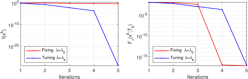
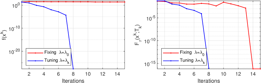
Figure 1: Two strategies for setting $\lambda$ in NL0R for solving Example 4.1. The sub-figures in the top (bottom) row are produced by NL0R under $s_{*}=100$ ($s_{*}=500$).

To see the performance of NL0R under fixing $\lambda=\lambda_{0}$ or updating $\lambda=\lambda_{k}$, two instances of Example 4.1 are tested and according results are shown in Figure 1. It can be clearly seen that $\|F_{\tau_{k}}({\rm x}^{k};T_{k})\|$ declines dramatically for both fixing $\lambda=\lambda_{0}$ and updating $\lambda=\lambda_{k}$, indicating NL0R enjoys a quadratic convergence property. While the objective $f({\rm x}^{k})$ produced by NL0R under fixing $\lambda=\lambda_{0}$ stabilizes at a level, which means it achieves a local minima. By contrast, NL0R under updating $\lambda=\lambda_{k}$ delivers the objective $f({\rm x}^{k})$ that drops down sharply and approaches to a globally optimal value. Therefore, the updating rule makes NL0R perform better and thus is adopted to proceed with our numerical comparisons in the sequel.

4.2 Compressed sensing

CS has seen revolutionary advances both in theory and algorithm over the past decade. Ground-breaking papers that pioneered the advances are [23, 15, 16]. We will focus on two types of data: the randomly generated data and the 2-dimensional image data. For the first data, we consider the exact recovery ${\rm y}=A{\rm x}$, where the sensing matrix $A$ chosen as in [50, 56]. While for the image data, we consider the inexact recovery ${\rm y}=A{\rm x}+\xi$, where $\xi$ is the noise and $A$ will be described in Example 4.2.

Example 4.1 (Random data)

Let $A\in\mathbb{R}^{m\times n}$ be a random Gaussian matrix with each column being identically and independently distributed (iid) samples of the standard normal distribution. We then normalize each column to be a unit length. Next, the $s_{*}$ non-zero components of the ‘ground truth’ signal ${\rm x}^{*}$ are also iid samples of the standard normal distribution, and their locations are picked randomly. Finally, the measurement is given by ${\rm y}=A{\rm x}^{*}$.

Example 4.2 (2-D image data)

Some images are naturally not sparse themselves but could be sparse under some wavelet transforms. Here, we take advantage of the Daubechies wavelet 1, denoted as $W(\cdot)$. Then images under this transform (i.e., $x^{*}:=W(\omega)$) is sparse, $\omega$ be the vectorized intensity of an input image. Because of this, the explicit form of the sampling matrix may not be available. We consider a sampling matrix taking the form $A=FW^{-1}$, where $F$ is the partial fast Fourier transform, and $W^{-1}$ is the inverse of $W$. Finally, the added noise $\xi$ has each element $\xi_{i}\sim{\tt nf}\cdot\mathcal{N}$ with $\mathcal{N}$ being the standard normal distribution and ${\tt nf}$ being the noise factor. Three typical choices of ${\tt nf}$ are taken into account, namely ${\tt nf}\in\{0.01,0.05,0.1\}$. For this experiment, we compute a gray image (see the original image in Figure 3) with size $512\times 512$ (i.e. $n=512^{2}=262144$) and the sampling size $m=20033$ and $29729$ respectively.

4.2.1 Comparisons for random data

Since a large number of state-of-the-art methods have been proposed to solve the CS problems, it is far beyond our scope to compare all of them. To make comparisons fair, we only focus on those algorithms (often referred as regularized methods) which aim at solving (1.1) or its relaxations, where $\ell_{0}$ norm is replaced by some approximations such as $\ell_{q}(0<q\leq 1)$ [32] or $\ell_{1}-\ell_{2}$ [34]. Note that greedy methods mentioned in Subsection 1.1, for the model (1.2) with $s$ being given, have been famous for the super-fast computational speed and the high order of accuracy when $s$ is relatively small to $n$. However, we will not compare them with NL0R since we would like to consider the scenario when $s$ is unknown. We select MIRL1 [56], AWL1 [34, ADMM for weighted $\ell_{1-2}$] which is a faster approximation of the method proposed in [50], IRSLQ [32] (we choose $q=1/2$) and PDASC [31]. All parameters are set as default except for setting the maximum iteration number as 100 and removing the final refinement step for MRIL1 and del=1e-8 for PDASC. Note that PDASC and NL0R are the second-order methods and the other three belong to the category of the first-order methods.

To see the accuracy of the solutions and the speed of these five methods, we run 20 trials with medium dimensions $n$ increasing from 10000 to 30000 and keeping $m=\lceil 0.25n\rceil,s_{*}=\lceil 0.01n\rceil$ or $s_{*}=\lceil 0.05n\rceil$. Average results are reported in Figure 2, where $s_{*}=\lceil 0.01n\rceil$, and Table 1, where $s_{*}=\lceil 0.05n\rceil$. As shown in Figure 2, NL0R always generates the smallest $\|{\rm x}-{\rm x}^{*}\|$, the most accurate recovery, with accuracy order at least $10^{-14}$, followed by PDSAC. By contrast, the other three methods get accuracy with the order being above $10^{-5}$. This phenomenon well testifies that the second-order methods have their advantages in producing a higher order of accuracy. When it comes to the computational speed, it can be clearly seen that NL0R always runs the fastest, with only consuming about 2 seconds when $n=30000$. PDSAC is the runner up. This shows that, for problems in higher dimensions, NL0R and PDSAC are able to run faster than the first-order methods. Similar observations can be seen in Table 1. In a nutshell, NL0R delivers the most accurate recovery within the shortest computational time.

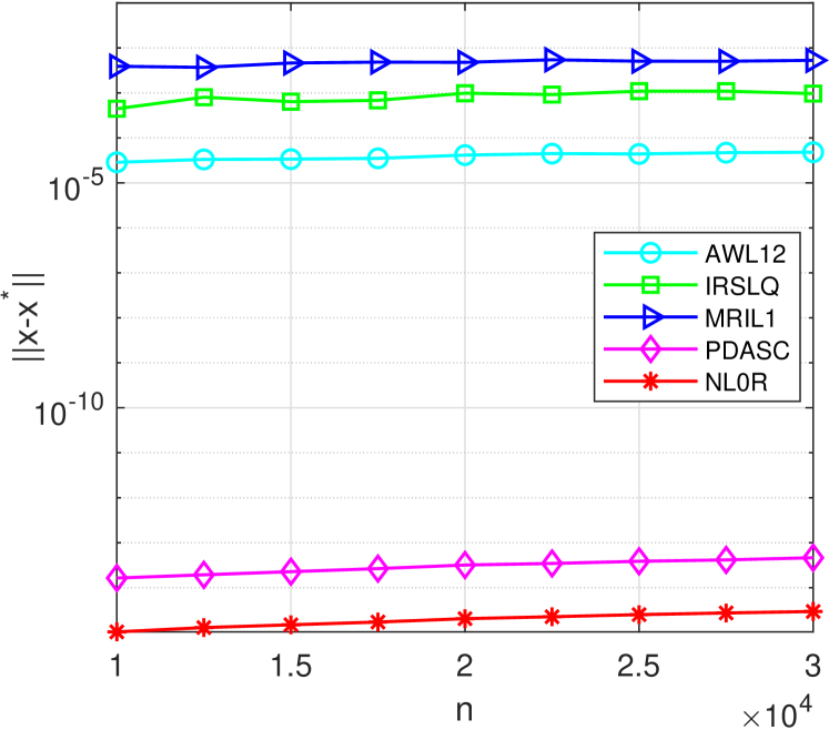
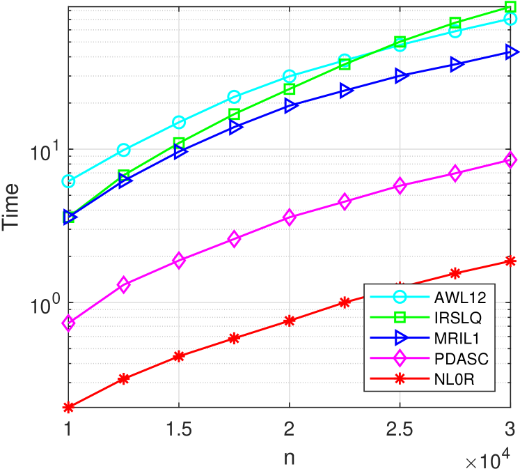
Figure 2: Average recovery error and time of five methods for solving Example 4.1.

Table 1: Performance of five methods for Example 4.1.

	$\|{\rm x}-{\rm x}^{*}\|$						Time (in seconds)
n	10000	15000	20000	25000	30000		10000	15000	20000	25000	30000
AWL12	8.39e-05	1.10e-04	1.21e-04	1.32e-04	1.43e-04		17.71	42.70	85.46	133.3	195.4
RSLQ	3.79e-04	4.32e-04	4.05e-04	3.58e-04	6.25e-04		7.653	23.84	56.38	113.1	189.3
MRIL1	1.57e-02	1.96e-02	2.48e-02	2.63e-02	2.54e-02		4.595	12.00	23.21	36.93	52.36
PDASC	5.36e-14	7.81e-14	1.07e-13	1.33e-13	1.59e-13		0.972	2.290	4.680	7.514	11.12
SNL0	1.16e-14	6.58e-15	2.37e-14	2.96e-14	3.55e-14		0.602	1.363	2.549	4.175	6.303

4.2.2 Comparisons for 2-D image data

In Example 4.2, data size $n$ is relatively large, which possibly makes most regularized methods suffer extremely slow computation. Hence, we select three greedy methods CSMP (denoted for CoSaMP) [38], HTP [28] and AIHT [11] as well as PDSCA. As suggested in package PDSCA, we set another rule to stop each method if at $k$th iteration it satisfies $\|A{\rm x}^{k}-y\|\leq\|A{\rm x}^{*}-y\|$ to speed up the termination. Moreover, to make comparisons fair, we fist run PDSCA, which is capable of delivering a solution with a good sparsity level $s$. Then we set this sparsity level $s$ for CSMP, HTP and AIHT since they need such prior information. Let ${\rm x}$ be a solution produced by a method. Apart from reporting the sparsity level $\|{\rm x}\|_{0}$ and the CPU time of a method, we also compute the peak signal to noise ratio (PSNR) defined by

$${\rm PSNR}:=10\log_{10}(n\|{\rm x}-{\rm x}^{*}\|^{-2})$$

to measure the performance of the method. Note that the larger PSNR is, the much closer ${\rm x}$ approaches to the true image ${\rm x}^{*}$, namely the better performance of a method yields. Results for Example 4.2 are presented in Figure 3 and Table 2 , where SPDSA offers the biggest PSNR when nf$=0.01$, whilst NL0R produces the biggest ones when nf$=0.05$ and nf$=0.1$, which means our method is more robust to the noise. In addition, NL0R  runs the fastest and renders the sparsest representations for most cases.

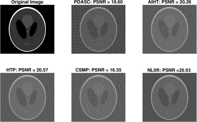
Figure 3: Recovery results for Example 4.2 with $m=20033$ and nf$=0.1$.

Table 2: Performance of five methods for Example 4.2.

		nf$=0.01$				nf$=0.05$				nf$=0.1$
		PSNR	Time	$\|{\rm x}\|_{0}$		PSNR	Time	$\|{\rm x}\|_{0}$		PSNR	Time	$\|{\rm x}\|_{0}$
	SPDSA	21.62	15.53	9716		20.11	8.45	5982		19.60	5.72	2969
$m=20033$	AIHT	19.81	148.5	9716		20.15	2.23	5982		20.26	19.3	2969
$n=262144$	HTP	19.66	19.15	9716		20.27	3.40	5982		20.57	3.41	2969
	SCMP	12.49	51.54	9716		18.44	63.1	5982		16.35	14.8	2969
	NL0R	23.21	7.130	9690		21.91	4.43	4173		20.93	3.07	2803
	SPDSA	35.37	11.54	9902		25.07	6.58	5002		22.61	5.44	3513
$m=29729$	AIHT	32.21	71.42	9902		24.78	9.52	5002		23.07	9.16	3513
$n=262144$	HTP	34.89	14.38	9902		25.14	4.57	5002		23.19	2.02	3513
	SCMP	21.48	39.79	9902		23.00	9.94	5002		20.73	2.26	3513
	NL0R	33.59	6.761	8787		25.31	3.99	3885		23.23	2.58	2641

4.3 Sparse linear complementarity problem

Sparse linear complementarity problems have been applied into dealing with real-world applications such as bimatrix games and portfolio selection problems [19, 49, 42]. The problem aims at finding a sparse vector ${\rm x}\in\mathbb{R}^{n}$ from $\Omega:=\{{\rm x}\in\mathbb{R}^{n}:~{}{\rm x}\geq 0,\ M{\rm x}+q\geq 0,\ \langle{\rm x},M{\rm x}+q\rangle=0\},$ where $M\in\mathbb{R}^{n\times n}$ and $q\in\mathbb{R}^{n}$. A point ${\rm x}\in\Omega$ is equivalent to

(4.2) $$f(x) := \sum_{i=1}^{n}\phi(x_{i},M_{i}{\rm x}+q_{i})=0,$$

where $\phi$ is the so-called NCP function, which is defined by $\phi(a,b)=0$ if and only if $a\geq 0,b\geq 0,ab=0$. We take advantage of an NCP function $\phi(a,b)=a_{+}^{2}b_{+}^{2}+(-a)_{+}^{2}+(-b)_{+}^{2}$, where $a_{+}:=\max\{a,0\}$, and a testing example from [54].

Example 4.3

Let $M=ZZ^{\top}$ with $Z\in\mathbb{R}^{n\times m}$ and $m\leq n$ (e.g. $m=n/2$). Elements of $Z$ are iid samples from the standard normal distribution. Each column is then normalized to have a unit length. The ‘ground truth’ sparse solution ${\rm x}^{*}$ with a sparsity level $s_{*}$ is produced the same as in Example 4.1 and $q$ is obtained by $q_{i}=-(M{\rm x}^{*})_{i}$ if $x_{i}^{*}>0$ and $q_{i}=|(M{\rm x}^{*})_{i}|$ otherwise.

Since there are very few methods that have been proposed to process the sparse LCP, we only select two solvers: the half-thresholding projection (HTP) method [43] and LEMKA’s method (LEMKE). We alter the sample size $n$ but fix $m=n/2,s_{*}=0.01n$ and $s_{*}=0.05n$. Average results over 20 trials are reported in Figure 4 where $s_{*}=0.01n$ and Table 3 where $s_{*}=0.05n$. Comparing with HTP, LEMKE and NL0R produce much more accurate solutions since their obtained objective function values $f({\rm x})$ and the recovered accuracy $\|{\rm x}-{\rm x}^{*}\|$ almost tend to zero. When it comes to the computational speed, the picture is significantly different. As shown in Figure 4, NL0R runs super-fast, followed by LEMKE, and HTP comes the last. Similar observations can be seen in Table 3, where for the case of $n=20000$, NL0R only consumes about 8.826 seconds while LEMKE takes 531.1 seconds and HTP needs 207.9 seconds. Therefore, NL0R evidently outperforms the others in the high dimensional settings.

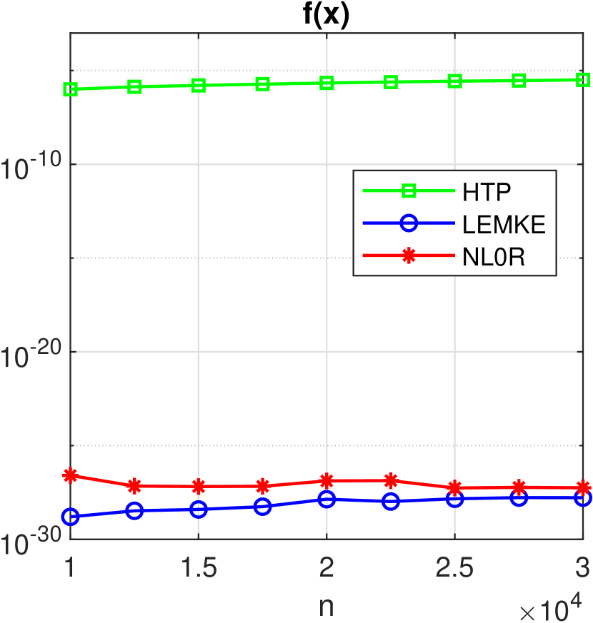
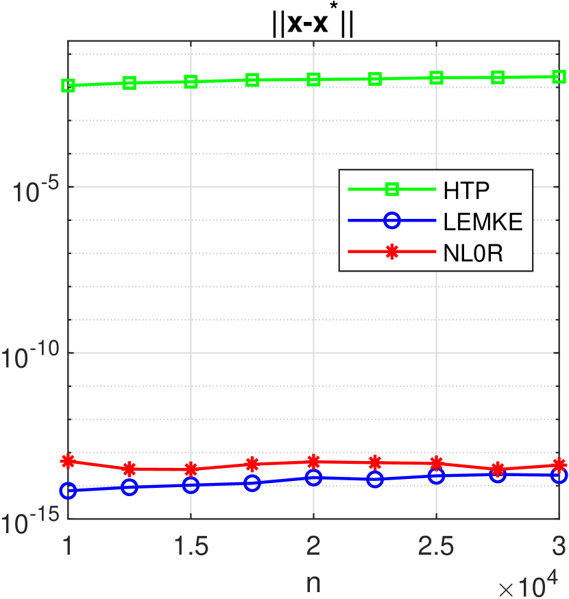
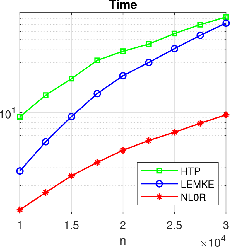
Figure 4: Performance of NL0R effected by $\lambda_{0}$ for solving Example 4.3.

Table 3: Performance of three methods for Example 4.3.

	$f({\rm x})$				$\|{\rm x}-{\rm x}^{*}\|$				Time (in seconds)
$n$	HTP	LEMKE	NL0R		HTP	LEMKE	NL0R		HTP	LEMKE	NL0R
5000	2.52e-06	1.15e-28	1.94e-27		5.55e-02	2.05e-14	6.46e-14		11.83	7.911	0.581
7500	4.20e-06	3.22e-28	3.84e-28		7.04e-02	3.15e-14	4.01e-14		27.69	27.14	1.240
10000	5.38e-06	7.21e-28	3.33e-27		8.36e-02	4.58e-14	9.88e-14		50.71	64.64	2.216
12500	6.76e-06	9.06e-28	4.00e-28		8.87e-02	5.10e-14	3.18e-14		79.96	127.7	3.434
15000	7.99e-06	1.18e-27	8.83e-28		9.86e-02	6.80e-14	6.07e-14		114.7	221.1	4.994
17500	9.30e-06	2.19e-27	8.37e-28		1.08e-01	7.69e-14	4.23e-14		158.4	354.0	6.862
20000	1.12e-05	3.22e-27	9.71e-27		1.18e-01	1.10e-13	2.72e-13		207.9	531.1	8.826

5 Conclusion

A vast body of work has developed numerical methods that only make use of the first-order information of the involved functions. Because of this, they are able to run fast but suffer from slow convergence. When Newton steps are integrated into some of these methods, then much more rapid convergence can be achieved. To the best of our knowledge, the current theoretic guarantees include two groups: either the (sub)sequence converges to a stationary point of $\ell_{0}$-regularized optimization or the distance between each iterate and any given sparse reference point is bounded by an error bound in the sense of probability. However, those do not thoroughly reveal the reasons why those methods with Newton steps perform exceptionally well. In this paper, we designed a Newton-type method for the $\ell_{0}$-regularized optimization and proved that the generated sequence converges to a stationary point globally and quadratically. This well explains such a method is expected to enjoy an appealing performance from the theoretical perspective, which was testified by the numerical experiments where it is capable of rendering a relatively high order of accuracy with fast computational speed.

References

- [1] H. Attouch, J. Bolte, and B. F. Svaiter. Convergence of descent methods for semi-algebraic and tame problems: proximal algorithms, forward–backward splitting, and regularized gauss–seidel methods. Mathematical Programming, 137(1-2):91–129, 2013.
- [2] S. Bahmani, B. Raj, and P. T. Boufounos. Greedy sparsity constrained optimization. Journal of Machine Learning Research, 14(Mar):807–841, 2013.
- [3] C. Bao, B. Dong, L. Hou, Z. Shen, X. Zhang, and X. Zhang. Image restoration by minimizing zero norm of wavelet frame coefficients. Inverse Problems, 32(11):115004, 2016.
- [4] A. Beck and Y. C. Eldar. Sparsity constrained nonlinear optimization: Optimality conditions and algorithms. SIAM Journal on Optimization, 23(3):1480–1509, 2013.
- [5] A. Beck and N. Hallak. Proximal mapping for symmetric penalty and sparsity. SIAM Journal on Optimization, 28(1):496–527, 2018.
- [6] D. Bertsimas, A. King, and R. Mazumder. Best subset selection via a modern optimization lens. The Annals of Statistics, pages 813–852, 2016.
- [7] W. Bian and X. Chen. Smoothing neural network for constrained non-Lipschitz optimization with applications. IEEE Transactions on Neural Networks and Learning Systems, 23(3):399–411, 2012.
- [8] W. Bian and X. Chen. Linearly constrained non-Lipschitz optimization for image restoration. SIAM Journal on Imaging Sciences, 8(4):2294–2322, 2015.
- [9] W. Bian and X. Chen. A smoothing proximal gradient algorithm for nonsmooth convex regression with cardinality penalty. SIAM Journal on Numerical Analysis, 58(1):858–883, 2020.
- [10] J. D. Blanchard, J. Tanner, and K. Wei. CGIHT: conjugate gradient iterative hard thresholding for compressed sensing and matrix completion. Information and Inference: A Journal of the IMA, 4(4):289–327, 2015.
- [11] T. Blumensath. Accelerated iterative hard thresholding. Signal Processing, 92(3):752–756, 2012.
- [12] T. Blumensath and M. E. Davies. Gradient pursuits. IEEE Transactions on Signal Processing, 56(6):2370–2382, 2008.
- [13] T. Blumensath and M. E. Davies. Iterative thresholding for sparse approximations. Journal of Fourier analysis and Applications, 14(5-6):629–654, 2008.
- [14] T. Blumensath and M. E. Davies. Normalized iterative hard thresholding: Guaranteed stability and performance. IEEE Journal of Selected Topics in Signal Processing, 4(2):298–309, 2010.
- [15] E. J. Candès, J. Romberg, and T. Tao. Robust uncertainty principles: Exact signal reconstruction from highly incomplete frequency information. IEEE Transactions on Information Theory, 52(2):489–509, 2006.
- [16] E. J. Candès and T. Tao. Decoding by linear programming. IEEE Transactions on Information Theory, 51(12):4203–4215, 2005.
- [17] X. Chen, M. K. Ng, and C. Zhang. Non-Lipschitz -regularization and box constrained model for image restoration. IEEE Transactions on Image Processing, 21(12):4709–4721, 2012.
- [18] W. Cheng, Z. Chen, and Q. Hu. An active set Barzilar-Borwein algorithm for regularized optimization. Journal of Global Optimization, 2019.
- [19] R. W. Cottle. Linear complementarity problem. Springer, 2009.
- [20] W. Dai and O. Milenkovic. Subspace pursuit for compressive sensing signal reconstruction. IEEE transactions on Information Theory, 55(5):2230–2249, 2009.
- [21] T. De Luca, F. Facchinei, and C. Kanzow. A semismooth equation approach to the solution of nonlinear complementarity problems. Mathematical Programming, 75(3):407–439, 1996.
- [22] T. Dinh, B. Wang, A. L. Bertozzi, S. J. Osher, and J. Xin. Sparsity meets robustness: channel pruning for the feynman-kac formalism principled robust deep neural nets. arXiv preprint arXiv:2003.00631, 2020.
- [23] D. L. Donoho. Compressed sensing. IEEE Transactions on Information Theory, 52(4):1289–1306, 2006.
- [24] M. Elad. Sparse and redundant representations: from theory to applications in signal and image processing. Springer Science & Business Media, 2010.
- [25] M. Elad, M. A. Figueiredo, and Y. Ma. On the role of sparse and redundant representations in image processing. Proceedings of the IEEE, 98(6):972–982, 2010.
- [26] F. Facchinei. Minimization of sc1 functions and the maratos effect. Operations Research Letters, 17(3):131–138, 1995.
- [27] F. Facchinei and C. Kanzow. A nonsmooth inexact newton method for the solution of large-scale nonlinear complementarity problems. Mathematical Programming, 76(3):493–512, 1997.
- [28] S. Foucart. Hard thresholding pursuit: an algorithm for compressive sensing. SIAM Journal on Numerical Analysis, 49(6):2543–2563, 2011.
- [29] J. Huang, Y. Jiao, Y. Liu, and X. Lu. A constructive approach to l0 penalized regression. The Journal of Machine Learning Research, 19(1):403–439, 2018.
- [30] K. Ito and K. Kunisch. A variational approach to sparsity optimization based on lagrange multiplier theory. Inverse Problems, 30(1):015001, 2013.
- [31] Y. Jiao, B. Jin, and X. Lu. A primal dual active set with continuation algorithm for the -regularized optimization problem. Applied and Computational Harmonic Analysis, 39(3):400–426, 2015.
- [32] M.-J. Lai, Y. Xu, and W. Yin. Improved iteratively reweighted least squares for unconstrained smoothed minimization. SIAM Journal on Numerical Analysis, 51(2):927–957, 2013.
- [33] S. Lin, R. Ji, Y. Li, C. Deng, and X. Li. Toward compact convnets via structure-sparsity regularized filter pruning. IEEE Transactions on Neural Networks and Learning Systems, 2019.
- [34] Y. Lou and M. Yan. Fast minimization via a proximal operator. Journal of Scientific Computing, 74(2):767–785, 2018.
- [35] Z. Lu. Iterative hard thresholding methods for regularized convex cone programming. Mathematical Programming, 147(1-2):125–154, 2014.
- [36] Z. Lu and Y. Zhang. Sparse approximation via penalty decomposition methods. SIAM Journal on Optimization, 23(4):2448–2478, 2013.
- [37] J. J. Moré and D. C. Sorensen. Computing a trust region step. SIAM Journal on Scientific and Statistical Computing, 4(3):553–572, 1983.
- [38] D. Needell and J. A. Tropp. Cosamp: Iterative signal recovery from incomplete and inaccurate samples. Applied and Computational Harmonic Analysis, 26(3):301–321, 2009.
- [39] L. Pan, S. Zhou, N. Xiu, and H.-D. Qi. A convergent iterative hard thresholding for nonnegative sparsity optimization. Pacific Journal of Optimization, 13(2):325–353, 2017.
- [40] Y. C. Pati, R. Rezaiifar, and P. S. Krishnaprasad. Orthogonal matching pursuit: Recursive function approximation with applications to wavelet decomposition. In Signals, Systems and Computers, 1993. 1993 Conference Record of The Twenty-Seventh Asilomar Conference on, pages 40–44. IEEE, 1993.
- [41] A. Patrascu, I. Necoara, and P. Patrinos. A proximal alternating minimization method for -regularized nonlinear optimization problems: Application to state estimation. Proceedings of the IEEE Conference on Decision and Control, 2015:4254–4259, 2015.
- [42] M. Shang, C. Zhang, and N. Xiu. Minimal zero norm solutions of linear complementarity problems. Journal of Optimization Theory and Applications, 163(3):795–814, 2014.
- [43] M. Shang, S. Zhou, and N. Xiu. Extragradient thresholding methods for sparse solutions of co-coercive ncps. Journal of Inequalities and Applications, 2015(1):34, 2015.
- [44] E. Soubies, L. Blanc-Féraud, and G. Aubert. A continuous exact penalty (cel0) for least squares regularized problem. SIAM Journal on Imaging Sciences, 8(3):1607–1639, 2015.
- [45] C. Soussen, J. Idier, J. Duan, and D. Brie. Homotopy based algorithms for -regularized least squares. IEEE Transactions on Signal Processing, 63(13):3301–3316, 2015.
- [46] J. A. Tropp. Just relax: Convex programming methods for identifying sparse signals in noise. IEEE Transactions on Information Theory, 52(3):1030–1051, 2006.
- [47] J. A. Tropp and A. C. Gilbert. Signal recovery from random measurements via orthogonal matching pursuit. IEEE Transactions on Information Theory, 53(12):4655–4666, 2007.
- [48] J. Wright, Y. Ma, J. Mairal, G. Sapiro, T. S. Huang, and S. Yan. Sparse representation for computer vision and pattern recognition. Proceedings of the IEEE, 98(6):1031–1044, 2010.
- [49] J. Xie, S. He, and S. Zhang. Randomized portfolio selection with constraints. Pacific Journal of Optimization, 4(1):89–112, 2008.
- [50] P. Yin, Y. Lou, Q. He, and J. Xin. Minimization of 1-2 for compressed sensing. SIAM Journal on Scientific Computing, 37(1):A536–A563, 2015.
- [51] X.-T. Yuan, P. Li, and T. Zhang. Gradient hard thresholding pursuit. The Journal of Machine Learning Research, 18(1):6027–6069, 2017.
- [52] X.-T. Yuan and Q. Liu. Newton greedy pursuit: A quadratic approximation method for sparsity-constrained optimization. In Proceedings of the IEEE Conference on Computer Vision and Pattern Recognition, pages 4122–4129, 2014.
- [53] X.-T. Yuan, X. Liu, and S. Yan. Visual classification with multitask joint sparse representation. IEEE Transactions on Image Processing, 21(10):4349–4360, 2012.
- [54] S. Zhou, M. Shang, L. Pan, and M. Li. Newton hard thresholding pursuit for sparse lcp via a new merit function. arXiv preprint arXiv:2004.02244, 2020.
- [55] S. Zhou, N. Xiu, and H.-D. Qi. Global and quadratic convergence of Newton hard-thresholding pursuit. arXiv preprint arXiv:1901.02763, 2019.
- [56] S. Zhou, N. Xiu, Y. Wang, L. Kong, and H.-D. Qi. A null-space-based weighted minimization approach to compressed sensing. Information and Inference: A Journal of the IMA, 5(1):76–102, 2016.