Estimation Of all parameters in the Fractional Ornstein-Uhlenbeck model under discrete observations

Abstract.

Let the Ornstein-Uhlenbeck process $(X_{t})_{t\geq 0}$ driven by a fractional Brownian motion $B^{H}$, described by $dX_{t}=-\theta X_{t}dt+\sigma dB_{t}^{H}$ be observed at discrete time instants $t_{k}=kh$, $k=0,1,2,\cdots,2n+2$. We propose ergodic type statistical estimators $\hat{\theta}_{n}$, $\hat{H}_{n}$ and $\hat{\sigma}_{n}$ to estimate all the parameters $\theta$, $H$ and $\sigma$ in the above Ornstein-Uhlenbeck model simultaneously. We prove the strong consistence and the rate of convergence of the estimators. The step size $h$ can be arbitrarily fixed and will not be forced to go zero, which is usually a reality. The tools to use are the generalized moment approach (via ergodic theorem) and the Malliavin calculus.

1. Introduction

The Ornstein-Uhlenbeck process $(X_{t})_{t\geq 0}$ is described by the following Langevin equation:

$$dX_{t}=-\theta X_{t}dt+\sigma\text{d}B_{t}^{H}\,,$$ (1.1)

where $\theta>0$ so that the process is ergodic and where for simplicity of the presentation we assume $X_{0}=0$. Other initial value can be treated exactly in the same way. We assume that the process $(X_{t})_{t\geq 0}$ is observed at discrete time instants $t_{k}=kh$ and we want to use the observations $\{X_{h},X_{2h},\cdots,X_{2n+2)h}\}$ to estimate the parameters $\theta$, $H$ and $\sigma$ appeared in the above Langevin equation simultaneously.

Before we continue let us briefly recall some recent relevant works obtained in literature. Most of the works are concerned with the estimator of the drift parameter $\theta$. When the Ornstein-Uhlenbeck process $(X_{t})_{t\geq 0}$ can be observed continuously and when the parameters $\sigma$ and $H$ are assumed to be known, we have the following works.

• The maximum likelihood estimator for $\theta$ defined by $\theta_{T}^{{\rm mle}}$ is studied [12] (see also the references therein for earlier references), and is proved to be strongly consistent. The asymptotic behavior of the bias and the mean square of $\theta_{T}^{{\rm mle}}$ is also given. In this paper, a strongly consistent estimator of $\sigma$ is also proposed.

• A least squares estimator defined by $\tilde{\theta}_{T}=\frac{-\int_{0}^{T}X_{t}dX_{t}}{\int_{0}^{T}X_{t}^{2}}$ was studied in [3, 7, 8]. It is proved that $\tilde{\theta}_{T}\rightarrow\theta$ almost surely as $T\rightarrow\infty$. It is also proved that when $H<\leq 3/4$, $\sqrt{T}(\tilde{\theta}_{T}-\theta)$ converges in law to a mean zero normal random variable. The variance of this normal variable is also obtained. When $H\geq 3/4$, the rate of convergence is also known [8].

Usually in reality the process can only be observed at discrete times $\{t_{k}=kh,k=1,2,\cdots,n\}$ for some fixed observation time lag $h>0$. In this very interesting case, there are very limited works. Let us only mention two ([9, 11]). To the best of knowledge there is only one work [2] to estimate all the parameters $\theta$, $H$ and ${\sigma}$ in the same time, where the observations are assumed to be made continuously.

The diffusion coefficient ${\sigma}$ represents the “volatility” and it is commonly believed that it should be computed (hence estimated) by the $1/H$ variations (see [8] and references therein). To use the $1/H$ variations one has to assume the process can be observed continuously (or we have high frequency data). Namely, it is a common belief that $\sigma$ can only be estimated when one has high frequency data.

In this work, we assume that the process can only be observed at discrete times $\{t_{k}=kh,k=1,2,\cdots,n\}$ for some fixed observation time lag $h>0$ (without the requirement that $h\rightarrow 0$). We want to estimate $\theta$, $H$ and ${\sigma}$ simultaneously. The idea we use is the ergodic theorem, namely, we find the explicit form of the limit distribution of $\frac{1}{n}\sum_{k=1}^{n}f(X_{kh})$ and use it to estimate our parameters. People may naturally think that if we appropriately choose three different $f$, then we may obtain three different equations to obtain all the three parameters $\theta$, $H$ and ${\sigma}$.

However, this is impossible since as long as we proceed this way, we shall find out that whatever we choose $f$, we cannot get independent equations. Motivated by a recent work [4], we may try to add the limit distribution of $\frac{1}{n}\sum_{k=1}^{n}g(X_{kh},X_{(k+1)h})$ to find all the parameters. However, this is still impossible because regardless how we choose $f$ and $g$ we obtain only two independent equations. This is because regardless how we choose $f$ and $g$ the limits depends only on the covariance of the limiting Gaussians (see $Y_{0}$ and $Y_{h}$ ulteriorly). Finally, we propose to use the following quantities to estimate all the three parameters $\theta$, $H$ and ${\sigma}$:

$$\frac{\sum_{k=1}^{n}X_{kh}^{2}}{n},\quad\frac{\sum_{k=1}^{n}X_{kh}X_{(kh+h}}{n},\quad\frac{\sum_{k=1}^{n}X_{2kh}X_{2kh+2h}}{n}.$$ (1.2)

We shall study the strong consistence and joint limiting law of our estimators.

The paper is organized as follows. In Section 2, we recall some known results. The construction and the strong consistency of the estimators are provided in Section 3. Central limit theorems are obtained in Section 4. To make the paper more readable, we delay some proofs in Append A. To use our estimators we need the determinant of some functions to be nondegenerate. This is given in Appendix B. Some numerical simulations to validate our estimators are illustrated in Appendix C.

2. Preliminaries

Let $(\Omega,\mathcal{F},\mathbb{P})$ be a complete probability space. The expectation on this space is denoted by $\mathbb{E}$. The fractional Brownian motion $(B_{t}^{H},t\in\mathbb{R})$ with Hurst parameter $H\in(0,1)$ is a zero mean Gaussian process with the following covariance structure:

$$\mathbb{E}(B_{t}^{H}B_{s}^{H})=R_{H}(t,s)=\frac{1}{2}(\mid t\mid^{2H}+\mid s\mid^{2H}+\mid t-s\mid^{2H}).$$ (2.3)

On stochastic analysis of this fractional Brownian motion, such as stochastic integral $\int_{a}^{b}f(t)dB_{t}^{H}$, chaos expansion, and stochastic differential equation $dX_{t}=b(X_{t})dt+{\sigma}(X_{t})dB_{t}^{H}$ we refer to [1].

For any $s,t\geq 0$, we define

$$\langle I_{[0,t]},I_{[0,s]}\rangle_{\mathcal{H}}=R_{H}(s,t)\,.$$ (2.4)

We can first extend this scalar product to general elementary functions $f(\cdot)=\sum_{i=1}^{n}a_{i}I_{[0,s_{i}]}(\cdot)$ by (bi-)linearity and then to general function by a limiting argument. We can then obtain the reproducing kernel Hilbert space, denoted by $\mathcal{H}$, associated with this Gaussian process $B_{t}^{H}$ (see e.g. [7] for more details).

Let $\mathcal{S}$ be the space of smooth and cylindrical random variables of the form

$$F=f(B^{H}(\phi_{1}),....,B^{H}(\phi_{n})),\quad\phi_{1},...,\phi_{n}\in C^{\infty}_{0}([0,T]),$$

where $f\in C_{b}^{\infty}(\mathbf{R}^{n})$ and $B^{H}(\phi)=\int_{0}^{\infty}\phi(t)dB_{t}^{H}$. For such a variable $F$, we define its Malliavin derivative as the $\mathcal{H}$ valued random element:

$$DF=\sum_{k=1}^{n}\frac{\partial f}{\partial x_{i}}(B^{H}(\phi_{1}),...,B^{H}(\phi_{n}))\phi_{i}.$$

We shall use the following result in Section 4 to obtain the central limit theorem. We refer to [6] and many other references for a proof.

Proposition 2.1.

Let $\{F_{n},n\geq 1\}$ be a sequence of random variables in the space of $p$th Wiener Chaos, $p\geq 2$ ,such that $\lim_{n\rightarrow\infty}\mathbb{E}(F_{n}^{2})=\sigma^{2}$. Then the following statements are equivalent:

• $F_{n}$ converges in law to $N(0,\sigma^{2})$ as $n$ tends to infinity.

• $\|DF_{n}\|_{\mathcal{H}}^{2}$ converges in $L^{2}$ to a constant as n tends to infinity.

3. Estimators of $\theta$,$H$ and $\sigma$

If $X_{0}=0$, then the solution $X_{t}$ to (1.1) can be expressed as

$$X_{t}=\sigma\int_{0}^{t}e^{-\theta(t-s)}\text{d}B^{H}_{s}.$$ (3.5)

The associated stationary solution, the solution of (1.1) with the the initial value

$$Y_{0}=\int_{-\infty}^{0}e^{\theta s}\text{d}B_{s}\,,$$ (3.6)

can be expressed as

$$Y_{t}=\int_{-\infty}^{t}e^{-\theta(t-s)}\text{d}B_{s}=e^{-\theta t}Y_{0}+X_{t}$$ (3.7)

and has the same distribution as the limiting normal distribution of $X_{t}$ (when $t\rightarrow\infty$). Let’s consider the following two quantities :

$$\left\{\begin{array}[]{lll}\eta_{n}=\frac{1}{n}\sum_{k=1}^{n}X_{kh}^{2},\\ \eta_{h,n}=\frac{1}{n}\sum_{k=1}^{n}X_{kh}X_{kh+h}\,,\\ \eta_{2h,n}=\frac{1}{n}\sum_{k=1}^{n}X_{2kh}X_{2kh+2h}\,.\end{array}\right.$$ (3.8)

As in [5] or [9], we have the following ergodic result:

$$\lim_{n\rightarrow\infty}\eta_{n}=\mathbb{E}(Y_{0}^{2})=\sigma^{2}\frac{\Gamma(2H+1)\sin(\pi H)}{2\pi}\int_{-\infty}^{\infty}\frac{\mid x\mid^{1-2H}}{\theta^{2}+x^{2}}dx\,.$$ (3.9)

Now we want to have a similar result for $\eta_{h,n}$. First, let’s study the ergodicity of the processes $\{Y_{t+h}-Y_{t}\}_{t\geq 0}$. According to [10], a centered Gaussian wide-sense stationary process $M_{t}$ is ergodic if $\mathbb{E}(M_{t}M_{0})\rightarrow 0$ as $t$ tends to infinity. We shall apply this result to $M_{t}=Y_{t+h}-Y_{t}\,,t\geq 0$. Obviously, it is a centered Gaussian stationary process and

$$\mathbb{E}((Y_{t+h}-Y_{t})(Y_{h}-Y_{0}))=\mathbb{E}(Y_{t+h}Y_{h})-\mathbb{E}(Y_{t+h}Y_{0})-\mathbb{E}(Y_{t}Y_{h})+\mathbb{E}(Y_{t}Y_{0})\,.$$

In [5, Theorem 2.3], it is proved that $\mathbb{E}(Y_{t}Y_{0})\rightarrow 0$ as $t$ goes to infinity. Thus, it is easy to see that $\mathbb{E}((Y_{t+h}-Y_{t})(Y_{h}-Y_{0}))\rightarrow 0$. Hence, we see that the process $\{Y_{t+h}-Y_{t}\}_{t\geq 0}$ is ergodic. This implies

$$\frac{\sum_{k=1}^{n}\large{[}Y_{(k+1)h}-Y_{kh}\large{]^{2}}}{n}\rightarrow_{n\rightarrow\infty}\mathbb{E}([Y_{h}-Y_{0}]^{2})\,.$$

This combined with (3.9) yields the following Lemma.

Theorem 3.1.

Let $\eta_{n}$, $\eta_{h,n}$ and $\eta_{2h,n}$ be defined by (3.8). Then as $n\rightarrow\infty$ we have

$$\lim_{n\rightarrow\infty}\eta_{n} = \mathbb{E}(Y_{0}^{2})=\sigma^{2}\frac{\Gamma(2H+1)\sin(\pi H)}{2\pi}\int_{-\infty}^{\infty}\frac{\mid x\mid^{1-2H}}{\theta^{2}+x^{2}}dx\,;$$ (3.10)

$$\lim_{n\rightarrow\infty}\eta_{h,n} = \mathbb{E}(Y_{0}Y_{h})=\sigma^{2}\frac{\Gamma(2H+1)\sin(\pi H)}{2\pi}\int_{-\infty}^{\infty}e^{ixh}\frac{\mid x\mid^{1-2H}}{\theta^{2}+x^{2}}dx\,;$$ (3.11)

$$\lim_{n\rightarrow\infty}\eta_{2h,n} = \mathbb{E}(Y_{0}Y_{2h})=\sigma^{2}\frac{\Gamma(2H+1)\sin(\pi H)}{2\pi}\int_{-\infty}^{\infty}e^{2ixh}\frac{\mid x\mid^{1-2H}}{\theta^{2}+x^{2}}dx\,.$$

From the above theorem we propose the following construction for the estimators of the parameters ${\theta}$, $H$ and ${\sigma}$.

First let us define

$$\left\{\begin{array}[]{lll}f_{1}(\sigma,\theta,H):=\frac{1}{2\pi}\sigma^{2}\Gamma(2H+1)\sin(\pi H)\int_{0}^{\infty}\frac{x^{1-2H}}{\theta^{2}+x^{2}}dx\,;\\ f_{2}(\sigma,\theta,H):=\frac{1}{2\pi}\sigma^{2}\Gamma(2H+1)\sin(\pi H)\int_{0}^{\infty}\cos(hx)\frac{x^{1-2H}}{\theta^{2}+x^{2}}dx\,;\\ f_{3}(\sigma,\theta,H):=\frac{1}{2\pi}\sigma^{2}\Gamma(2H+1)\sin(\pi H\int_{0}^{\infty}\cos(2hx)\frac{x^{1-2H}}{\theta^{2}+x^{2}}dx\end{array}\right.$$ (3.13)

and let $f(\theta,H,\sigma)=(f_{1}(\sigma,\theta,H),f_{2}(\sigma,\theta,H),f_{3}(\sigma,\theta,H))^{T}$.

Then we set

$$\left\{\begin{array}[]{lll}f_{1}(\sigma,\theta,H)=\eta_{n}=\frac{1}{n}\sum_{k=1}^{n}X_{kh}^{2}\,;\\ f_{2}(\sigma,\theta,H)=\eta_{h,n}=\frac{1}{n}\sum_{k=1}^{n}X_{kh}X_{kh+h}\,;\\ f_{3}(\sigma,\theta,H)=\eta_{2h,n}=\frac{1}{n}\sum_{k=1}^{n}X_{2kh}X_{2kh+2h}\,.\end{array}\right.$$ (3.14)

This is a system of three equations for three unknowns $({\theta},H,{\sigma})$. If the determinant of the Jacobian (of $f$)

$$J({\theta},H,{\sigma})=\left(\begin{matrix}\frac{\partial f_{1}({\theta},H,{\sigma})}{\partial{\theta}}&\frac{\partial f_{1}({\theta},H,{\sigma})}{\partial H}&\frac{\partial f_{1}({\theta},H,{\sigma})}{\partial{\sigma}}\\ \frac{\partial f_{2}({\theta},H,{\sigma})}{\partial{\theta}}&\frac{\partial f_{2}({\theta},H,{\sigma})}{\partial H}&\frac{\partial f_{2}({\theta},H,{\sigma})}{\partial{\sigma}}\\ \frac{\partial f_{3}({\theta},H,{\sigma})}{\partial{\theta}}&\frac{\partial f_{3}({\theta},H,{\sigma})}{\partial H}&\frac{\partial f_{3}({\theta},H,{\sigma})}{\partial{\sigma}}\\ \end{matrix}\right)\$$ (3.15)

is not zero at $({\theta}_{0},H_{0},{\sigma}_{0})$, then the above equation (3.14) has a unique solution $(\tilde{\theta}_{n},\tilde{H}_{n},\tilde{\sigma}_{n})$ in the neighborhood of $({\theta}_{0},H_{0},{\sigma}_{0})$ (We will discuss the determinant $J({\theta},H,{\sigma})$ in Appendix B). Namely, $(\tilde{\theta}_{n},\tilde{H}_{n},\tilde{\sigma}_{n})$ satisfies

$$\left\{\begin{array}[]{lll}f_{1}(\tilde{\theta}_{n},\tilde{H}_{n},\tilde{\sigma}_{n})=\eta_{n}=\frac{1}{n}\sum_{k=1}^{n}X_{kh}^{2}\,;\\ f_{2}(\tilde{\theta}_{n},\tilde{H}_{n},\tilde{\sigma}_{n})=\eta_{h,n}=\frac{1}{n}\sum_{k=1}^{n}X_{kh}X_{kh+h}\,;\\ f_{3}(\tilde{\theta}_{n},\tilde{H}_{n},\tilde{\sigma}_{n})=\eta_{2h,n}=\frac{1}{n}\sum_{k=1}^{n}X_{2kh}X_{2kh+2h}\,.\end{array}\right.$$

Or we can write as

$$(\tilde{\theta}_{n},\tilde{H}_{n},\tilde{\sigma}_{n})^{T}=f^{-1}(\Upupsilon_{n})\,,$$ (3.16)

where $f^{-1}$ is the inverse function of $f$ (if it exists) and

$$\Upupsilon_{n}=(\eta_{n},\eta_{h,n},\eta_{2h,n})^{T}\,.$$ (3.17)

We shall use $(\tilde{\theta}_{n},\tilde{H}_{n},\tilde{\sigma}_{n})$ to estimate the parameters $({\theta},H,{\sigma})$. We call $(\tilde{\theta}_{n},\tilde{H}_{n},\tilde{\sigma}_{n})$ the ergodic (or generalized moment) estimator of $({\theta},H,{\sigma})$.

It seems hard to explicitly obtain the explicit solution of the system of equation (3.14). However, it is a classical algebraic equations. There are numerous numeric approaches to find the approximate solution. We shall give some validation of our estimators numerically in Appendix C.

Since $f$ is a continuous function of $(\theta,H,\sigma)$ the inverse function $f^{-1}$ is also continuous if it exists. Thus we have the following a strong consistency result which is an immediate consequence of Theorem 3.1.

Theorem 3.2.

Assume (3.14) has a unique solution $(\tilde{\theta}_{n},\tilde{H}_{n},\tilde{\sigma}_{n})$. Then $(\tilde{\theta}_{n},\tilde{H}_{n},\tilde{\sigma}_{n})$ converge almost surely to $(\theta,H,\sigma)$ respectively as $n$ tends to infinity.

4. Central limit theorem

In this section, we shall concern with the central limit theorem associated with our ergodic estimator $(\tilde{\theta}_{n},\tilde{H}_{n},\tilde{\sigma}_{n})$. We shall prove that $\sqrt{n}(\tilde{\theta}_{n}-{\theta},\tilde{H}_{n}-H,\tilde{\sigma}_{n}-{\sigma})$ converge in law to a mean zero normal vector.

Let’s first consider the random variable $F_{n}$ defined by

$$F_{n}=\begin{pmatrix}\sqrt{n}(\eta_{n}-\mathbb{E}(\eta_{n}))\\ \sqrt{n}(\eta_{h,n}-\mathbb{E}(\eta_{h,n}))\\ \sqrt{n}(\eta_{2h,n}-\mathbb{E}(\eta_{2h,n}))\\ \end{pmatrix}.$$ (4.18)

Our first goal is to show that $F_{n}$ converges in law to a multivariate normal distribution using Proposition 2.1. So we consider a linear combination:

$$G_{n}=\alpha\sqrt{n}(\eta_{n}-\mathbb{E}(\eta_{n}))+\beta\sqrt{n}(\eta_{h,n}-\mathbb{E}(\eta_{h,n}))+\gamma\sqrt{n}(\eta_{2h,n}-\mathbb{E}(\eta_{2h,n})),$$ (4.19)

and show that it converges to a normal distribution.

We will use the following Feynman diagram formula [6], where interested readers can find a proof.

Proposition 4.1.

Let $X_{1},X_{2},X_{3},X_{4}$ be jointly Gaussian random variables with mean zero. Then

$$\mathbb{E}(X_{1}X_{2}X_{3}X_{4})=\mathbb{E}(X_{1}X_{2})\mathbb{E}(X_{3}X_{4})+\mathbb{E}(X_{1}X_{3})\mathbb{E}(X_{2}X_{4})+\mathbb{E}(X_{1}X_{4})\mathbb{E}(X_{2}X_{3})\,.$$

An immediate consequence of this result is

Proposition 4.2.

Let $X_{1},X_{2},X_{3},X_{4}$ be jointly Gaussian random variables with mean zero. Then

$$\mathbb{E}\left[(X_{1}X_{2}-\mathbb{E}(X_{1}X_{2}))(X_{3}X_{4}-\mathbb{E}(X_{3}X_{4}))\right]$$

$$\qquad\qquad=\mathbb{E}(X_{1}X_{3})\mathbb{E}(X_{2}X_{4})+\mathbb{E}(X_{1}X_{4})\mathbb{E}(X_{2}X_{3})\,;$$ (4.20)

$$\mathbb{E}\left[(X_{1}^{2}-\mathbb{E}(X_{1}^{2}))(X_{2}X_{3}-\mathbb{E}(X_{2}X_{3}))\right]=2\mathbb{E}(X_{1}X_{2})\mathbb{E}(X_{1}X_{3})\,;$$ (4.21)

$$\mathbb{E}\left[(X_{1}^{2}-\mathbb{E}(X_{1}^{2}))(X_{2}^{2}-\mathbb{E}(X_{2}^{2}))\right]=2\left[\mathbb{E}(X_{1}X_{2})\right]^{2}\,.$$ (4.22)

Theorem 4.3.

Let $H\in(0,\frac{1}{2})\cup(\frac{1}{2},\frac{3}{4})$. Let $X_{t}$ be the Ornstein-Uhlenbeck process defined by equation (1.1) and let $\eta_{n}$, $\eta_{h,n}$, $\eta_{2h,n}$ be defined by (3.8). Then

$$\begin{pmatrix}\sqrt{n}(\eta_{n}-\mathbb{E}(\eta_{n}))\\ \sqrt{n}(\eta_{h,n}-\mathbb{E}(\eta_{h,n}))\\ \sqrt{n}(\eta_{2h,n}-\mathbb{E}(\eta_{2h,n}))\\ \end{pmatrix}\rightarrow N(0,\Sigma),$$ (4.23)

where $\Sigma=\left(\Sigma(i,j)\right)_{1\leq i,j\leq 3}$ is a symmetric matrix whose elements are given by

$$\Sigma(1,1)=\Sigma(2,2)=\Sigma(3,3)=2\left[\mathbb{E}(Y_{0}^{2})\right]^{2}+4\sum_{m=0}^{\infty}\left[\mathbb{E}(Y_{0}Y_{mh})\right]^{2}\,;$$ (4.24)

$$\Sigma(1,2)=\Sigma(2,1)=\Sigma(2,3)=\Sigma(3,2)=4\sum_{m=0}^{\infty}\mathbb{E}(Y_{0}Y_{mh})\mathbb{E}(Y_{0}Y_{(m+1)h})\,;$$ (4.25)

$$\Sigma(1,3)=\Sigma(3,1)=4\sum_{m=0}^{\infty}\mathbb{E}(Y_{0}Y_{2mh})\mathbb{E}(Y_{0}Y_{2mh+2h})\,.$$ (4.26)

Remark 4.4.

1. It is easy from the following proof to see that all entries $\Sigma(i,j)$ of the covariance matrix $\Sigma$ are finite.

2. In an earlier work of Hu and Song it is said [9, Equation (19.19)] that the variance $\Sigma$ (corresponding to our $\Sigma(1,1)$ in our notation) is independent of the time lag $h$. But there was an error on the bound of $A_{n}$ on [9, page 434, line 14]. So, $A_{n}$ there does not go to zero. Its limit is re-calculated in this work.

3. It is clear that we can use $\tilde{\eta}_{2h,n}=\frac{1}{n}\sum_{k=1}^{n}X_{kh}X_{kh+2h}$ to replace $\eta_{2h,n}$.

4. We may use (3.10)-(LABEL:e.3.a8) to compute $\Sigma(i,j)\,,1\leq i,j\leq 3$ explicitly.

Proof  We write

$$\mathbb{E}(G_{n}^{2})=({\alpha},{\beta},{\gamma})\Sigma_{n}({\alpha},{\beta},{\gamma})^{T}\,,\quad\Sigma_{n}=\left(\Sigma_{n}(i,j)\right)_{1\leq i,j\leq 3}\,,$$

where $\Sigma_{n}$ is a symmetric $3\times 3$ matrix given by

$$\Sigma_{n}(1,1) =n\mathbb{E}\left[(\eta_{n}-\mathbb{E}(\eta_{n}))^{2}\right]\,;$$

$$\Sigma_{n}(1,2) =\Sigma_{n}(2,1)=n\mathbb{E}\left[(\eta_{n}-\mathbb{E}(\eta_{n}))(\eta_{h,n}-\mathbb{E}(\eta_{h,n}))\right]\,;$$

$$\Sigma_{n}(1,3) =\Sigma_{n}(3,1)=n\mathbb{E}\left[(\eta_{n}-\mathbb{E}(\eta_{n}))(\eta_{2h,n}-\mathbb{E}(\eta_{2h,n}))\right]\,;$$

$$\Sigma_{n}(2,2) =n\mathbb{E}\left[(\eta_{h,n}-\mathbb{E}(\eta_{h,n}))^{2}\right]\,;$$

$$\Sigma_{n}(2,3) =\Sigma_{n}(3,2)=n\mathbb{E}\left[(\eta_{h,n}-\mathbb{E}(\eta_{h,n}))(\eta_{2h,n}-\mathbb{E}(\eta_{2h,n}))\right]\,;$$

$$\Sigma_{n}(3,3) =n\mathbb{E}\left[(\eta_{2h,n}-\mathbb{E}(\eta_{2h,n}))^{2}\right]\,.$$

It is easy to observe that

1. the limits of $\Sigma_{n}(1,1)$, $\Sigma_{n}(2,2)$, and $\Sigma_{n}(3,3)$ are the same;

2. the limits of $\Sigma_{n}(1,2)$, and $\Sigma_{n}(2,3)$ are the same;

3. the limit of $\Sigma_{n}(1,3)$ can be obtained from the limit of $\Sigma_{n}(1,2)$ by replacing $h$ by $2h$;

4. the matrix is symmetric.

Thus, we only need to compute the limits of $\Sigma_{n}(1,1)$ and $\Sigma_{n}(1,2)$.

First, we compute the limit of $\Sigma_{n}(1,1)$. From the definition (3.8) of $\eta_{n}$ and Proposition 4.2, we have

$$\Sigma_{n}(1,1) = \frac{1}{n}\sum_{k,k^{\prime}=1}^{n}\mathbb{E}\left[(X_{kh}^{2}-\mathbb{E}\left[(X_{kh})^{2}\right])(X_{k^{\prime}h}^{2}-\mathbb{E}\left[(X_{k^{\prime}h})^{2}\right])\right]$$ (4.27)

$$= \frac{2}{n}\sum_{k,k^{\prime}=1}^{n}\left[\mathbb{E}(X_{kh}X_{k^{\prime}h})\right]^{2}$$

By Lemma A.2, we see that

$$\Sigma_{n}(1,1)\rightarrow\Sigma(1,1)=2\left[\mathbb{E}(Y_{0}^{2})\right]^{2}+4\sum_{m=0}^{\infty}\left[\mathbb{E}(Y_{0}Y_{mh})\right]^{2}\,.$$

This proves (4.24)

Now let consider the limit of $\Sigma_{n}(1,2)$. From the definitions (3.8) and from Proposition 4.2 it follows

$$\Sigma_{n}(1,2) = \frac{1}{n}\sum_{k,k^{\prime}=1}^{n}\mathbb{E}\left[(X_{kh}^{2}-\mathbb{E}\left[\left(X_{kh})^{2}\right]\right)\left(X_{k^{\prime}h}X_{(k^{\prime}+1)h}-\mathbb{E}\left[X_{k^{\prime}h}X_{(k^{\prime}+1)h}\right]\right)\right]$$ (4.28)

$$= \frac{2}{n}\sum_{k,k^{\prime}=1}^{n}\mathbb{E}(X_{kh}X_{k^{\prime}h})\mathbb{E}(X_{kh}X_{(k^{\prime}+1)h})\,.$$

By Lemma A.3, we have

$$\Sigma_{n}(1,2)\rightarrow 4\sum_{m=0}^{\infty}\mathbb{E}(Y_{0}Y_{mh})\mathbb{E}(Y_{0}Y_{(m+1)h})\,.$$ (4.29)

This proves (4.25). (4.26) is obtained from (4.25) by replacing $h$ by $2h$. This proves

$$\lim_{n\rightarrow\infty}\mathbb{E}(G_{n}^{2})=({\alpha},{\beta},{\gamma})\Sigma({\alpha},{\beta},{\gamma})^{T}\,.$$ (4.30)

Using Lemma A.4, we know that $J_{n}:=\langle DG_{n},DG_{n}\rangle_{\mathcal{H}}$ converges to a constant. Then by Proposition 2.1, we know $G_{n}$ converges in law to a normal random variable.

Since $G_{n}$ converges to a normal for any ${\alpha}$, ${\beta}$, and ${\gamma}$, we know by the Cramér-Wold theorem that $F_{n}$ converges to a mean zero Gaussian random vector, proving the theorem.   

Now using the delta method and the above Theorem 4.3 we immediately have the following theorem.

Theorem 4.5.

Let $H\in(0,\frac{1}{2})\cup(\frac{1}{2},\frac{3}{4})$. Let $X_{t}$ be the Ornstein-Uhlenbeck process defined by equation (1.1) and let $(\tilde{\theta}_{n},\tilde{H}_{n},\tilde{\sigma}_{n})$ be defined by (3.14). Then

$$\begin{pmatrix}\sqrt{n}(\tilde{\theta_{n}}-\theta)\\ \sqrt{n}(\tilde{H}_{n}-H)\\ \sqrt{n}(\tilde{\sigma}_{n}-{\sigma})\\ \end{pmatrix}{\stackrel{{\scriptstyle d}}{{\rightarrow}}}N(0,\tilde{\Sigma})\\ \,,$$

where $J$ denotes the Jacobian matrix of $f$, defined by (3.15), $\Sigma$ is defined in 4.3 and

$$\tilde{\Sigma}=\left[J({\theta},H,{\sigma})\right]^{-1}\Sigma\left[J^{T}({\theta},H,{\sigma})\right]^{-1}\,.$$ (4.31)

Appendix A Detailed computations

First, we need a lemma from [7, supplementary data, Lemma 5.4, Equation (5.7)].

Lemma A.1.

Let $X_{t}$ be the Ornstein-Uhlenbeck process defined by (1.1). Then

$$|\mathbb{E}(X_{t}X_{s})|\leq C(1\wedge|t-s|^{2H-2})\leq(1+|t-s|)^{2H-2}\,.$$ (A.32)

The above inequality also holds true for $Y_{t}$.

Lemma A.2.

Let $X_{t}$ be defined by (1.1). When $H\in(0,\frac{1}{2})\cup(\frac{1}{2},\frac{3}{4})$ we have

$$\lim_{n\rightarrow\infty}\frac{1}{n}\sum_{k,k^{\prime}=1}^{n}\left[\mathbb{E}(X_{kh}X_{k^{\prime}h})\right]^{2}=\left[\mathbb{E}(Y_{0}^{2})\right]^{2}+2\sum_{m=1}^{\infty}\left[\mathbb{E}(Y_{0}Y_{mh})\right]^{2}\,.$$ (A.33)

Proof  To simplify notations we shall use $X_{k}$, $Y_{k}$ to represent $X_{kh}$, $Y_{kh}$ etc. From the relation (3.7) it is easy to see that

$$\mathbb{E}(X_{k}X_{k^{\prime}}) = \mathbb{E}(Y_{k}Y_{k^{\prime}})-e^{-\theta k^{\prime}h}\mathbb{E}(Y_{0}Y_{k})-e^{-\theta kh}\mathbb{E}(Y_{0}Y_{k^{\prime}})+e^{-\theta(k+k^{\prime})h}\mathbb{E}(Y_{0}^{2})$$ (A.34)

$$=: \sum_{i=1}^{4}I_{i,k,k^{\prime}}\,,$$

where $I_{i,k,k^{\prime}}$, $i=1,\cdots,4$, denote the above $i$-th term.

Let us first consider $\frac{1}{n}\sum_{k,k^{\prime}=1}^{n}I_{i,k,k^{\prime}}^{2}$ for $i=2,3,4$. First, we consider $i=2$. By [5, Theorem 2.3], we know that $\mathbb{E}(Y_{0}Y_{k})$ converges to $0$ when $k\rightarrow\infty$. Thus by the Toeplitz theorem, we have

$$\frac{1}{n}\sum_{k,k^{\prime}=1}^{n}I_{2,k,k^{\prime}}^{2}=\frac{1}{n}\sum_{k,k^{\prime}=1}^{n}e^{-2\theta k^{\prime}h}\left[\mathbb{E}(Y_{0}Y_{k})\right]^{2}\leq C\frac{1}{n}\sum_{k}^{\infty}\left[\mathbb{E}(Y_{0}Y_{k})\right]^{2}\rightarrow 0\,.$$ (A.35)

Exactly in the same way we have

$$\frac{1}{n}\sum_{k,k^{\prime}=1}^{n}I_{3,k,k^{\prime}}^{2}\rightarrow 0\,.$$ (A.36)

When $i=4$, we have easily

$$\lim_{n\rightarrow\infty}\frac{1}{n}\sum_{k,k^{\prime}=1}^{n}I_{4,k,k^{\prime}}^{2}=\frac{1}{n}\sum_{k,k^{\prime}=1}^{n}e^{-2{\theta}(k+k^{\prime})}\left[\mathbb{E}(Y_{0}^{2})\right]^{2}\rightarrow 0\,.$$ (A.37)

Now we have

$$\frac{1}{n}\sum_{k,k^{\prime}=1}^{n}\left[\mathbb{E}(X_{k}X_{k^{\prime}})\right]^{2} = \frac{1}{n}\sum_{i,j=1}^{4}\sum_{k,k^{\prime}=1}^{n}I_{i,k,k^{\prime}}I_{j,k,k^{\prime}}$$

$$= \frac{1}{n}\sum_{k,k^{\prime}=1}^{n}I_{1,k,k^{\prime}}^{2}+\frac{1}{n}\sum_{i\not=1,{\rm or}j\not=1}\sum_{k,k^{\prime}=1}^{n}I_{i,k,k^{\prime}}I_{j,k,k^{\prime}}\,.$$

When one of the $i$ or $j$ is not equal to $1$, we have by the Hölder inequality

$$\frac{1}{n}\sum_{k,k^{\prime}=1}^{n}\left|I_{i,k,k^{\prime}}I_{j,k,k^{\prime}}\right| \leq \left(\frac{1}{n}\sum_{k,k^{\prime}=1}^{n}I_{i,k,k^{\prime}}^{2}\right)^{1/2}\left(\frac{1}{n}\sum_{k,k^{\prime}=1}^{n}I_{j,k,k^{\prime}}^{2}\right)^{1/2}$$

which will go to $0$ if we can show $\frac{1}{n}\sum_{k,k^{\prime}=1}^{n}I_{1,k,k^{\prime}}^{2},n=1,2,\cdots$ is bounded. In fact, we have

$$\frac{1}{n}\sum_{k,k^{\prime}=1}^{n}I_{1,k,k^{\prime}}=\frac{1}{n}\sum_{k,k^{\prime}=1}^{n}\left[\mathbb{E}(Y_{k}Y_{k^{\prime}})\right]^{2}$$

$$\qquad\quad=\frac{1}{n}\sum_{k,k^{\prime}=1}^{n}\left[\mathbb{E}(Y_{0}Y_{|k^{\prime}-k|})\right]^{2}$$

$$\qquad\quad=\mathbb{E}(Y_{0}^{2})+\frac{2}{n}\sum_{m=1}^{n-1}(n-m)\left[\mathbb{E}(Y_{0}Y_{m})\right]^{2}$$

$$\qquad\quad=\left[\mathbb{E}(Y_{0}^{2})\right]^{2}+2\sum_{m=1}^{n-1}\left[\mathbb{E}(Y_{0}Y_{m})\right]^{2}-\frac{2}{n}\sum_{m=1}^{n-1}m\left[\mathbb{E}(Y_{0}Y_{m})\right]^{2}\,.$$ (A.38)

By Lemma A.1 for $Y_{t}$ or an expression of $\mathbb{E}(Y_{0}Y_{m})$ given in [5, Theorem 2.3]:

$$\mathbb{E}(Y_{0}Y_{m})=\frac{1}{2}\sigma^{2}\sum_{n=1}^{N}(\Pi_{k=0}^{2n-1}(2H-k))m^{2H-2n}+O(m^{2H-2N-2})\,.$$

This means $\mathbb{E}(Y_{0}Y_{m})=O(m^{2H-2})$ as $m\rightarrow\infty$, which in turn means that $\left[\mathbb{E}(Y_{0}Y_{m})\right]^{2}=O(m^{4H-4})$. Hence, for $H<\frac{3}{4}$, $\sum_{m=0}^{n-1}\mathbb{E}(Y_{0}Y_{m})^{2}$ converges as $n$ tends to infinity.

Notice that for $H<\frac{3}{4}$, $m\mathbb{E}(Y_{0}Y_{m})^{2}=O(m^{4H-3})\rightarrow 0$ as $m\rightarrow\infty$. By Toeplitz theorem we have

$$\frac{1}{n}\sum_{m=0}^{n-1}m\left[\mathbb{E}(Y_{0}Y_{m})\right]^{2}\rightarrow 0\quad\hbox{as $n\rightarrow\infty$}\,.$$

Thus, $\frac{1}{n}\sum_{k,k^{\prime}>k}^{n}\left[\mathbb{E}(Y_{k}Y_{k^{\prime}})\right]^{2}$ converges to $\left[\mathbb{E}(Y_{0}^{2})\right]^{2}+2\sum_{m=1}^{\infty}\left[\mathbb{E}(Y_{0}Y_{m})\right]^{2}$ as $n$ tends to infinity.   

Lemma A.3.

Let $X_{t}$ be defined by (1.1). When $H\in(0,\frac{1}{2})\cup(\frac{1}{2},\frac{3}{4})$ we have

$$\lim_{n\rightarrow\infty}\frac{1}{n}\sum_{k,k^{\prime}=1}^{n}\mathbb{E}(X_{kh}X_{k^{\prime}h})\mathbb{E}(X_{kh}X_{(k^{\prime}+1)h})=2\sum_{m=0}^{\infty}\mathbb{E}(Y_{0}Y_{mh})\mathbb{E}(Y_{0}Y_{(m+1)h})\,.$$ (A.39)

Proof  We continue to use the notations in Lemma A.2.

$$\mathbb{E}(X_{k}X_{k^{\prime}}) = \sum_{i=1}^{4}I_{i,k,k^{\prime}}\,,$$

$$\mathbb{E}(X_{k}X_{k^{\prime}+1}) = \sum_{i=1}^{4}I_{i,k,k^{\prime}+1}\,,$$ (A.40)

where $I_{i,k,k^{\prime}}$, $i=1,\cdots,4$, is defined in (A.35). As in the proof of Lemma A.2, we have

$$\lim_{n\rightarrow\infty}\sum_{k,k^{\prime}=1}^{n}\mathbb{E}(X_{k}X_{k^{\prime}})\mathbb{E}(X_{k}X_{k^{\prime}+1})=\lim_{n\rightarrow\infty}\frac{1}{n}\sum_{k,k^{\prime}=1}^{n}\mathbb{E}(Y_{k}Y_{k^{\prime}})\mathbb{E}(Y_{k}Y_{k^{\prime}+1})$$

$$\qquad\quad=\frac{1}{n}\sum_{k,k^{\prime}=1}^{n}\mathbb{E}(Y_{0}Y_{|k^{\prime}-k|})\mathbb{E}(Y_{0}Y_{|k^{\prime}+1-k|})$$

$$\qquad\quad=\frac{1}{n}\sum_{m=0}^{n-1}(n-m)\mathbb{E}(Y_{0}Y_{m})\mathbb{E}(Y_{0}Y_{m+1})+\frac{1}{n}\sum_{m=1}^{n-1}(n-m)\mathbb{E}(Y_{0}Y_{m})\mathbb{E}(Y_{0}Y_{m-1})$$

Now we can use the same argument as in proof of Lemma A.2 to obtain

$$\lim_{n\rightarrow\infty}\sum_{k,k^{\prime}=1}^{n}\mathbb{E}(X_{k}X_{k^{\prime}})\mathbb{E}(X_{k}X_{k^{\prime}+1})=2\sum_{m=0}^{\infty}\mathbb{E}(Y_{0}Y_{m})\mathbb{E}(Y_{0}Y_{m+1})\,,$$

proving the lemma.   

Let $G_{n}$ be defined by (4.19) in Section 4. Its Malliavin derivative is given by

$$DG_{n} = \frac{1}{\sqrt{n}}2\alpha\sum_{k=1}^{n}X_{k}DX_{k}+\frac{1}{\sqrt{n}}\beta\sum_{k=1}^{n}(X_{k}DX_{k+1}+X_{k+1}DX_{k})$$ (A.41)

$$\qquad+\frac{1}{\sqrt{n}}\sum_{k=1}^{n}\gamma(X_{k}DX_{k+2}+X_{k+2}DX_{k})\,.$$

Lemma A.4.

Define the sequence of random variables $J_{n}:=\langle DG_{n},DG_{n}\rangle_{\mathcal{H}}$. Then

$$\lim_{n\rightarrow\infty}\mathbb{E}\left[J_{n}-\mathbb{E}(J_{n})\right]^{2}=0\,.$$ (A.42)

Proof  It is easy to see that $J_{n}$ is a linear combination of terms of the following forms (with the coefficients being a quadratic forms of ${\alpha},{\beta},{\gamma}$):

$$\tilde{J}_{n}:=\frac{1}{n}\sum_{k^{\prime},k=1}^{n}\langle DX_{k_{1}},DX_{k_{1}^{\prime}}\rangle_{\mathcal{H}}X_{k_{2}}X_{k_{2}^{\prime}}$$

$$\qquad=\frac{1}{n}\sum_{k^{\prime},k=1}^{n}\mathbb{E}(X_{k_{1}}X_{k_{1}^{\prime}})X_{k_{2}}X_{k_{2}^{\prime}}\,,$$ (A.43)

where $k_{1},k_{2}$ may take $k,k+1,k+2$, and $k_{1}^{\prime},k_{2}^{\prime}$ may take $k^{\prime},k^{\prime}+1,k^{\prime}+2$. For example, one term is to take $k_{1}=k_{2}=k$ and $k_{1}^{\prime}=k^{\prime}+1$, $k_{2}^{\prime}=k^{\prime}$ which corresponds to the product:

$$\langle\frac{1}{\sqrt{n}}2\alpha\sum_{k=1}^{n}X_{k}DX_{k},\frac{1}{\sqrt{n}}\beta\sum_{k=1}^{n}(X_{k}DX_{k+1}\rangle$$

$$\qquad\quad=\frac{2{\alpha}{\beta}}{n}\sum_{k^{\prime},k=1}^{n}\mathbb{E}(X_{k}X_{k^{\prime}+1})X_{k}X_{k^{\prime}}=:2{\alpha}{\beta}\tilde{J}_{0,n}\,.$$ (A.44)

We will first give a detail argument to explain why

$$\mathbb{E}\left[\tilde{J}_{0,n}-\mathbb{E}(\tilde{J}_{0,n})\right]^{2}\rightarrow 0$$

and then we outline the procedure that similar claims hold true for any terms in (A.43). Note that $\mathbb{E}(\tilde{J}_{0,n})$ will not converge to $0$.

From the Proposition 4.2 it follows

$$\mathbb{E}\left[\tilde{J}_{0,n}-\mathbb{E}(\tilde{J}_{0,n})\right]^{2} = \frac{1}{n^{2}}\sum_{k,k^{\prime},j,j^{\prime}=1}^{n}\mathbb{E}(X_{k}X_{k^{\prime}+1})\mathbb{E}(X_{j}X_{j^{\prime}+1})\mathbb{E}(X_{k}X_{j})\mathbb{E}(X_{k^{\prime}}X_{j^{\prime}})$$

$$\quad+\frac{1}{n^{2}}\sum_{k,k^{\prime},j,j^{\prime}=1}^{n}\mathbb{E}(X_{k}X_{k^{\prime}+1})\mathbb{E}(X_{j}X_{j^{\prime}+1})\mathbb{E}(X_{k}X_{j^{\prime}})\mathbb{E}(X_{k^{\prime}}X_{j})$$

$$=: I_{1,n}+I_{2,n}\,.$$

Using (A.32) we have

$$I_{1,n} \leq \frac{1}{n^{2}}\sum_{k,k^{\prime},j,j^{\prime}=1}^{n}(1+|k^{\prime}-k|)^{2H-2}(1+|j^{\prime}-j|)^{2H-2}$$

$$\qquad\quad(1+|j-k|)^{2H-2}(1+|k^{\prime}-j^{\prime}|)^{2H-2}\,;$$

$$I_{2,n} \leq \frac{1}{n^{2}}\sum_{k,k^{\prime},j,j^{\prime}=1}^{n}(1+|k^{\prime}-k|)^{2H-2}(1+|j^{\prime}-j|)^{2H-2}$$

$$\qquad\quad(1+|j^{\prime}-k|)^{2H-2}(1+|k^{\prime}-j|)^{2H-2}\,.$$

Now it is elementary to see that $I_{1,n}\rightarrow 0$ and $I_{2,n}\rightarrow 0$ when $n\rightarrow\infty$.

Now we deal with the general term

$$\tilde{J}_{1,n}:=\frac{1}{n}\sum_{k^{\prime},k=1}^{n}\mathbb{E}(X_{k_{1}}X_{k_{1}^{\prime}})X_{k_{2}}X_{k_{2}^{\prime}}$$

in (A.43), where $k_{1},k_{2}$ may take $k,k+1,k+2$, and $k_{1}^{\prime},k_{2}^{\prime}$ may take $k^{\prime},k^{\prime}+1,k^{\prime}+2$. We use Proposition 4.2 to obtain

$$\mathbb{E}\left[\tilde{J}_{1,n}-\mathbb{E}(\tilde{J}_{1,n})\right]^{2} = \frac{1}{n^{2}}\sum_{k,k^{\prime},j,j^{\prime}=1}^{n}\mathbb{E}(X_{k_{1}}X_{k_{1}^{\prime}})\mathbb{E}(X_{j_{1}}X_{j_{1}^{\prime}})\mathbb{E}(X_{k_{2}}X_{j_{2}})\mathbb{E}(X_{k_{2}^{\prime}}X_{j_{2}^{\prime}})$$

$$\quad+\frac{1}{n^{2}}\sum_{k,k^{\prime},j,j^{\prime}=1}^{n}\mathbb{E}(X_{k_{1}}X_{k_{1}^{\prime}})\mathbb{E}(X_{j_{1}}X_{j_{1}^{\prime}})\mathbb{E}(X_{k_{2}}X_{j_{2}^{\prime}})\mathbb{E}(X_{k_{2}^{\prime}}X_{j_{2}})$$

$$=: \tilde{I}_{1,n}+\tilde{I}_{2,n}\,,$$

where $k_{1},k_{2}$ may take $k,k+1,k+2$, and $k_{1}^{\prime},k_{2}^{\prime}$ may take $k^{\prime},k^{\prime}+1,k^{\prime}+2$, $j_{1},j_{2}$ may take $j,j+1,j+2$, and $j_{1}^{\prime},j_{2}^{\prime}$ may take $j^{\prime},j^{\prime}+1,j^{\prime}+2$. Using (A.32) we have

$$\tilde{I}_{1,n} \leq \frac{1}{n^{2}}\sum_{k,k^{\prime},j,j^{\prime}=1}^{n}(1+|k^{\prime}-k|)^{2H-2}(1+|j^{\prime}-j|)^{2H-2}$$

$$\qquad\quad(1+|j-k|)^{2H-2}(1+|k^{\prime}-j^{\prime}|)^{2H-2}\,;$$

$$\tilde{I}_{2,n} \leq \frac{1}{n^{2}}\sum_{k,k^{\prime},j,j^{\prime}=1}^{n}(1+|k^{\prime}-k|)^{2H-2}(1+|j^{\prime}-j|)^{2H-2}$$

$$\qquad\quad(1+|j^{\prime}-k|)^{2H-2}(1+|k^{\prime}-j|)^{2H-2}\,.$$

Now it is elementary to see that $I_{1,n}\rightarrow 0$ and $I_{2,n}\rightarrow 0$ when $n\rightarrow\infty$.   

Appendix B Determinant of the Jacobian of $f$

In this section we plot the determinant of the Jacobian of $J$. The determinant is plotted as a function of two parameters when the third one is fixed. Roughly, what these figures show is that the determinant will approach zero as $\theta$ goes to $\infty$ and as $\sigma$ goes to $0$ (See Fig 1 and Fig 2). They also show that the determinant becomes negative when $H$ is roughly smaller that $0.3$ or too close to $1$ (See Fig 3 and Fig 4).

Therefore, if we suppose that $0.3<H<\frac{3}{4}$, since the true value of the parameter $\theta$ is not infinite and $\sigma>0$, we should be able to say that the determinant of $J(\theta,H,\sigma)$ is positive in the neighborhood of $(\theta_{0},H_{0},\sigma_{0})$.

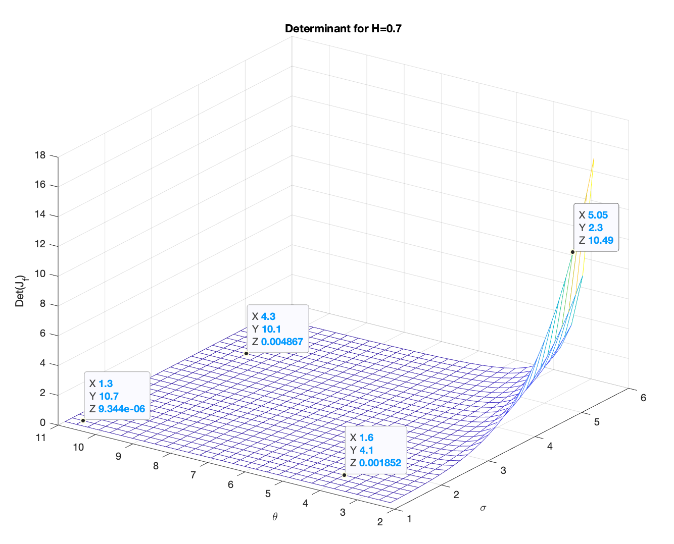
Figure 1. Determinant of the jacobian matrix of $f$ for $H=0.7$

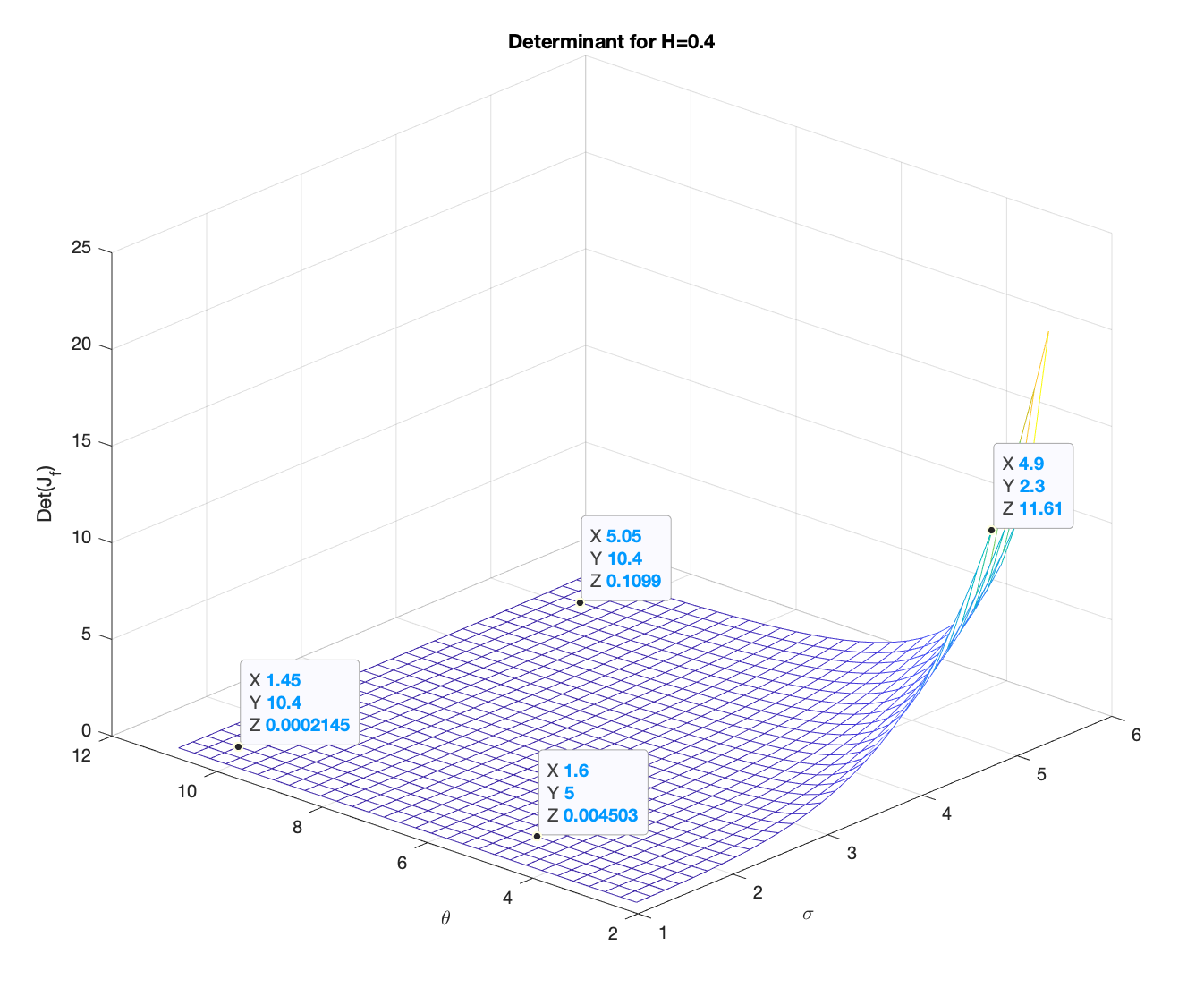
Figure 2. Determinant of the jacobian matrix of $f$ for $H=0.4$

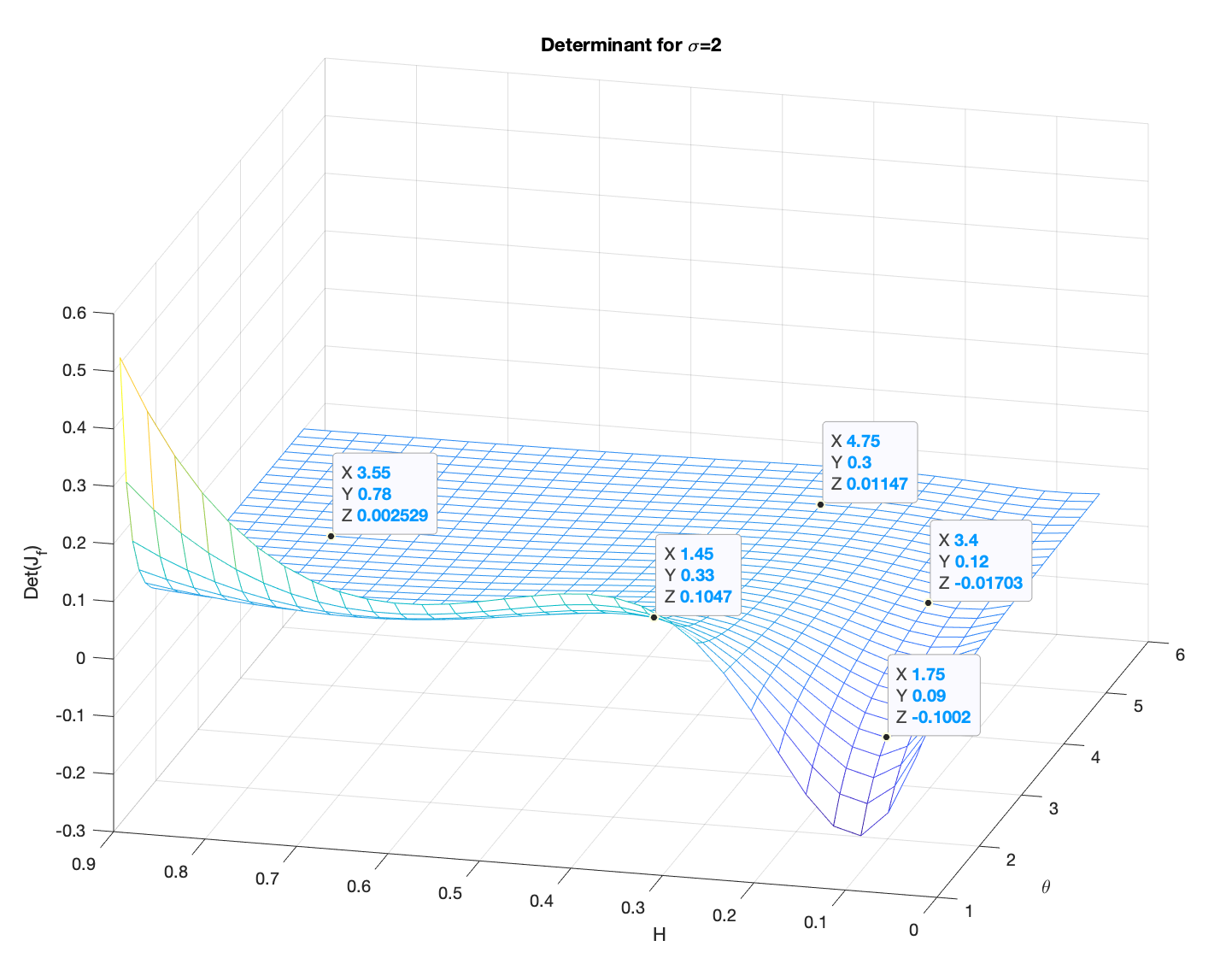
Figure 3. Determinant of the jacobian matrix of $f$ for $\sigma=2$

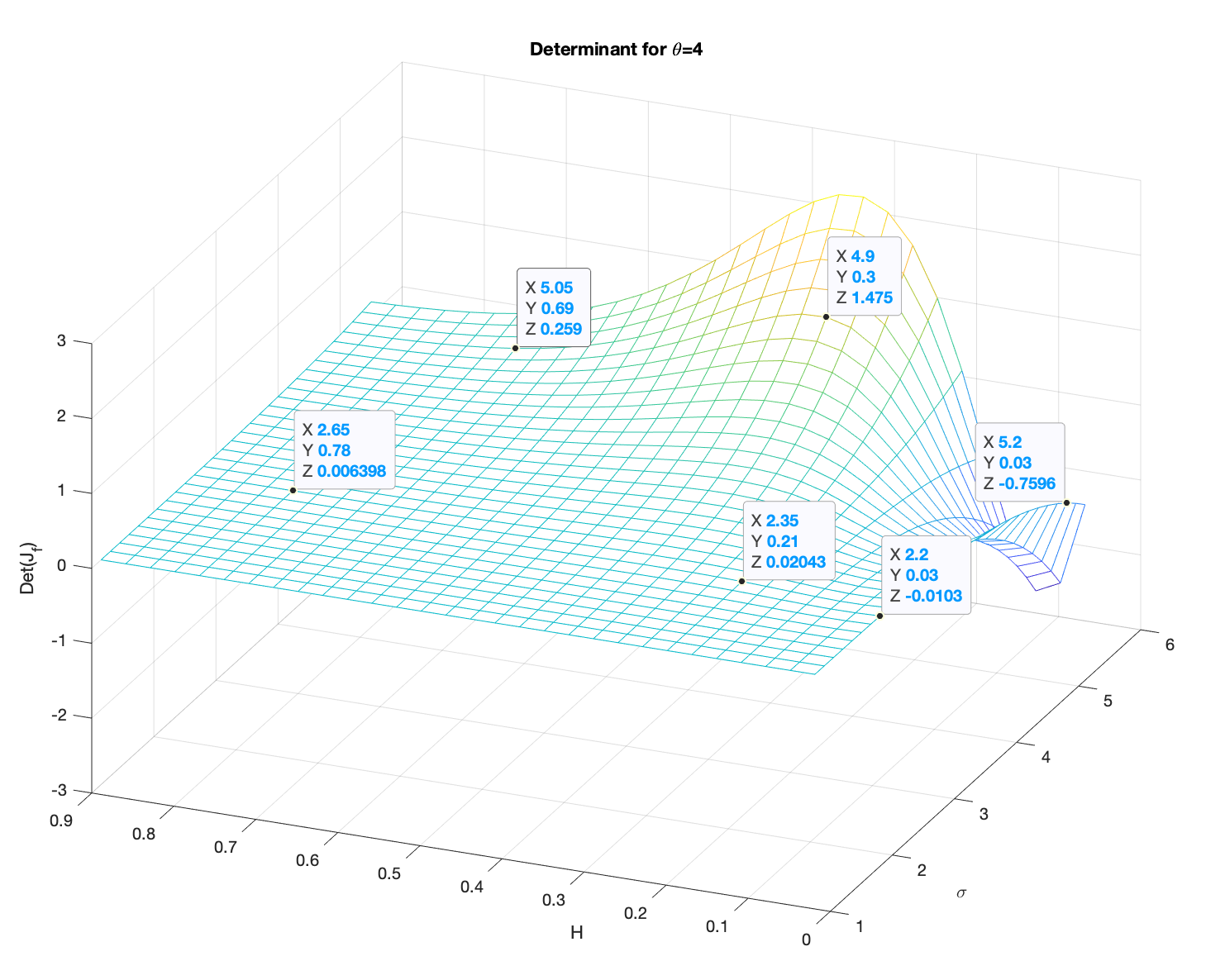
Figure 4. Determinant of the jacobian matrix of $f$ for $\theta=5$

Appendix C Numerical results

C.1. Strong consistency of the estimators

In this subsection, we illustrate the almost-sure convergence by plotting different trajectories of the estimators. We observe that when $log_{2}(n)\geq 14$, the estimators become very close to the true parameter.

However, since our estimators are random (they depend on the sample $\{X_{kh}\}_{k=1}^{n}$), what’s important to see in these figures is the deviations from the true parameter we are estimating. Even if three trajectories are not enough to make statements about the variance, the figures predict that the variance of $\tilde{\theta}_{n}$ is very high compared to the other estimators (see Fig 5 and Fig 6)and that, for $H$ close to $0$ (see Fig 7), the deviations of $\tilde{H}_{n}$ increase.

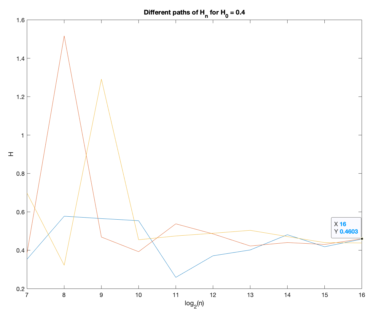
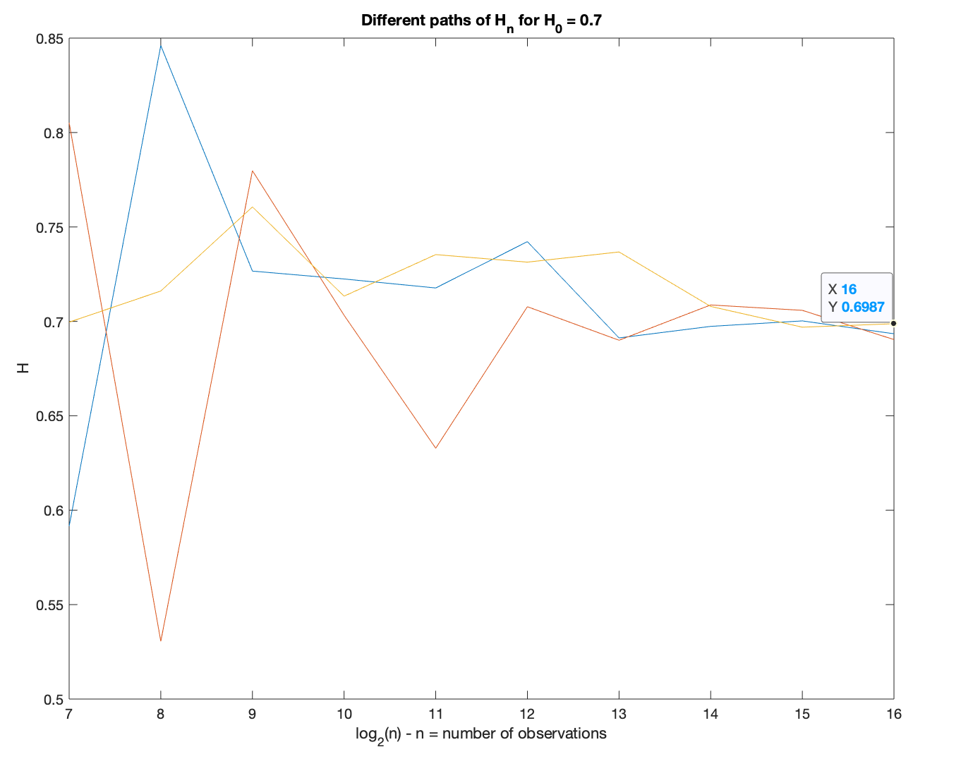
Figure 5. Convergence of $\widetilde{H_{n}}$ for $H=0.7$ and $H=0.4$

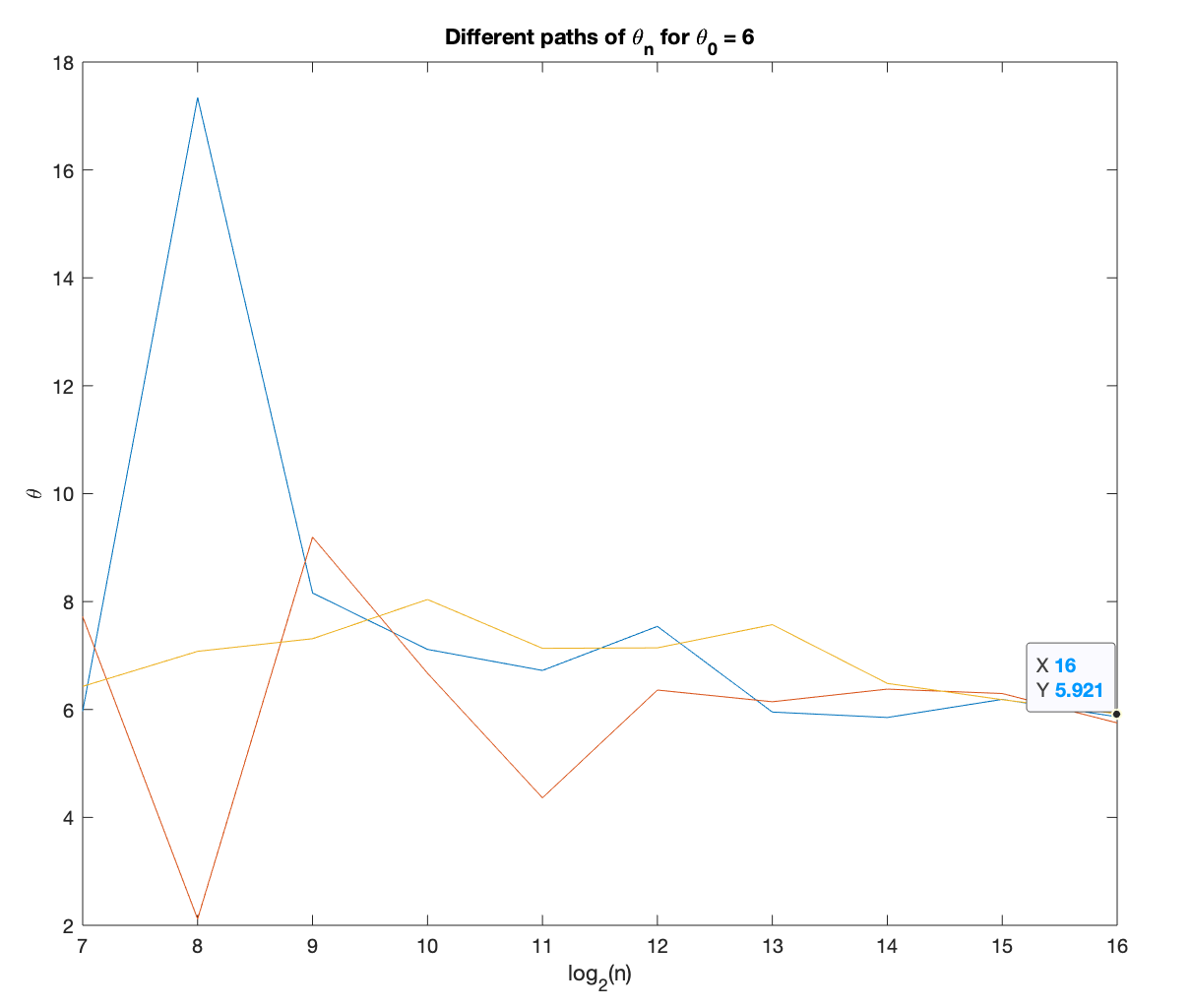
Figure 6. Convergence of $\widetilde{\theta_{n}}$ for $\theta=6$

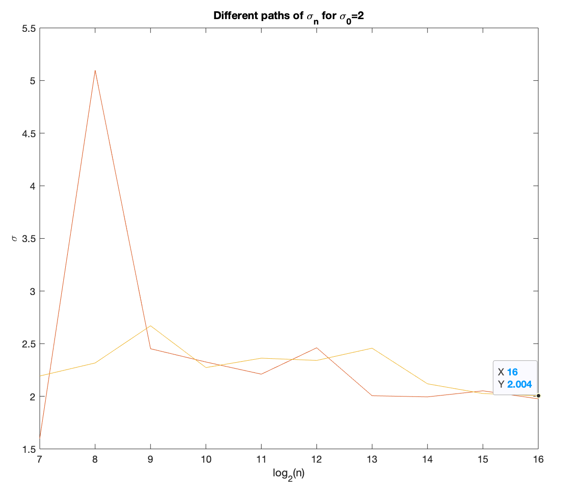
Figure 7. Convergence of $\widetilde{\sigma_{n}}$ for $\sigma=2$

C.2. Mean and standard deviation/Asymptotic behavior of the estimators

It is important to check the mean and deviation of our estimators. For example, a large variance implies a large deviation and therefore a “weak” estimator. That is why we plotted the mean and variance of our estimators for $n=2^{12}$ over $100$ samples.

As we observe, the standard deviation (s.d) of $\tilde{\theta}_{n}$ is larger than the s.d of $\tilde{sigma}_{n}$ which is larger than the s.d of $\tilde{H}_{n}$ (see table 1 and table 2). Notice also that the s.d of $\tilde{H}_{n}$ increases as $H$ decreases.

In [9], the variance of the $\theta$ estimator is proportional to $\theta^{2}$. In our case, it is difficult to compute the variances of our estimators (they depend on the matrix $\Sigma$ (see Theorem 4.3) and the Jacobian of the function $f$ (see equation (3.13)), however we should probably expect something similar which could explain the gap in the variances since the values of $\theta$ are usually bigger that the values taken by $\sigma$ or $H$.

Having access to $100$ estimates of each parameter, we are also able to plot the distributions of our estimators to show that they effectively have a Gaussian nature (4.5). (Fig 8, Fig 9 and Fig 10).

Table 1. $H=0.7$,$\theta=6$ and $\sigma=2$

	Mean	Standard deviation
$\widetilde{H_{n}}$	0.704	0.0221
$\widetilde{\theta_{n}}$	6.2983	0.8288
$\widetilde{\sigma_{n}}$	2.0921	0.2117

Table 2. $H=0.4$,$\theta=6$ and $\sigma=2$

	Mean	Standard deviation
$\widetilde{H_{n}}$	0.4392	0.0531
$\widetilde{\theta_{n}}$	6.832	1.3227
$\widetilde{\sigma_{n}}$	2.4785	0.3833

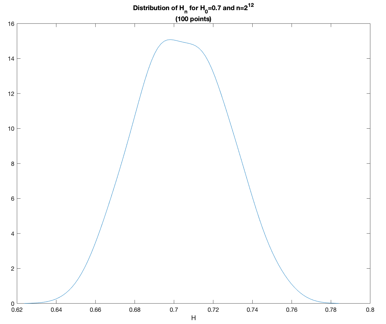
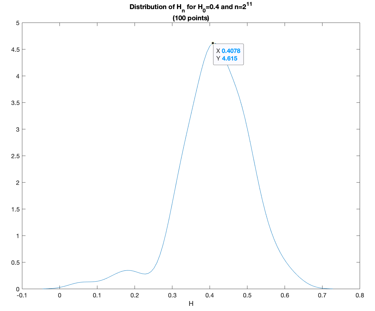
Figure 8. Distribution of $\widetilde{H_{n}}$ for $H=0.7$ and $H=0.4$

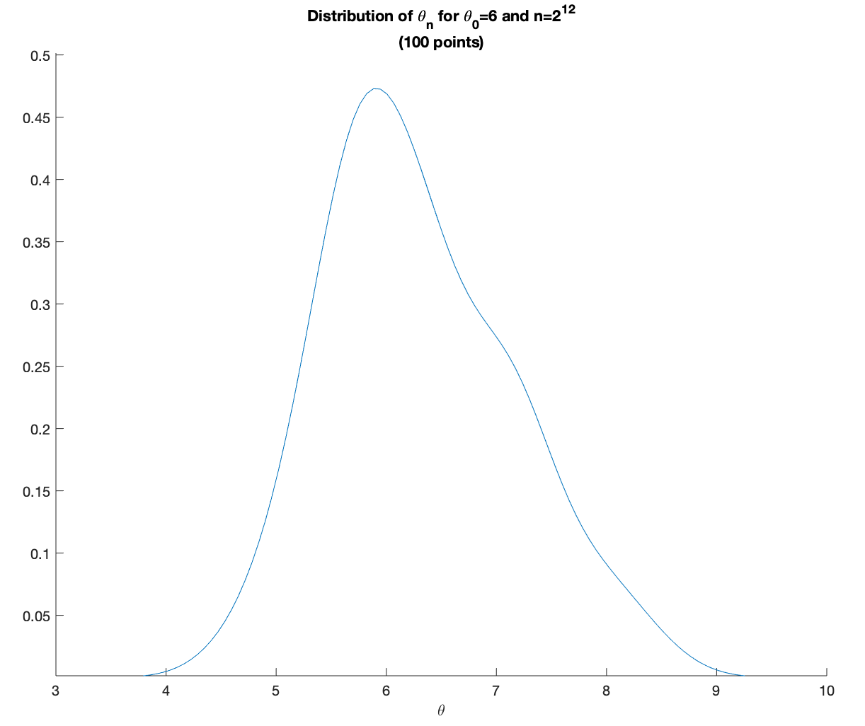
Figure 9. Distribution of $\widetilde{\theta_{n}}$ for $\theta=6$

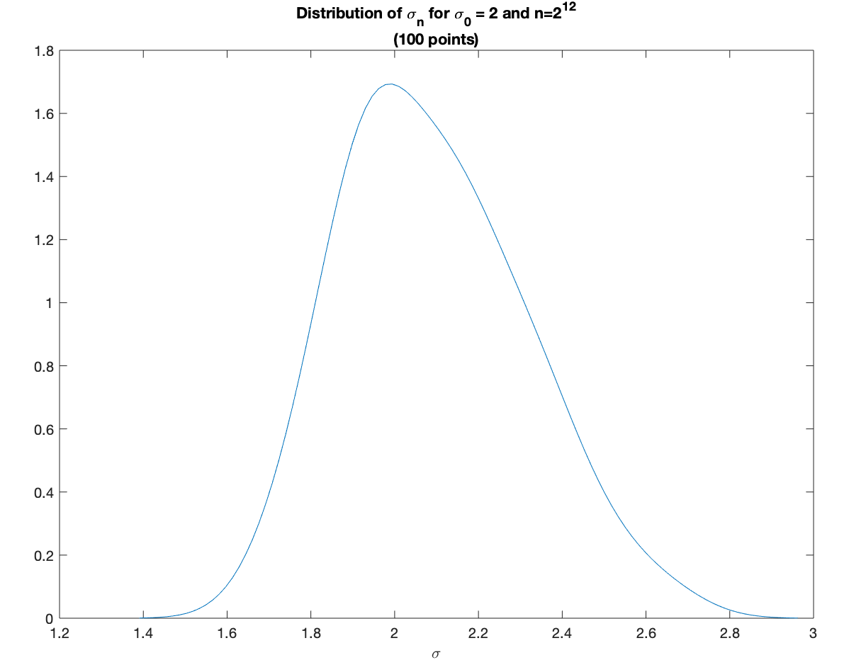
Figure 10. Distribution of $\widetilde{\sigma_{n}}$ for $\sigma=2$

References

• [1] F. Biagini, Y. Hu, B. Ø ksendal, and T. Zhang. Stochastic calculus for fractional Brownian motion and applications. Probability and its Applications (New York). Springer-Verlag London, Ltd., London, 2008.
• [2] A. Brouste and S. M. Iacus. Parameter estimation for the discretely observed fractional ornstein–uhlenbeck process and the yuima r package. Computational Statistics, 28(4):1529–1547, 2013.
• [3] Y. Chen, Y. Hu, and Z. Wang. Parameter estimation of complex fractional Ornstein-Uhlenbeck processes with fractional noise. ALEA Lat. Am. J. Probab. Math. Stat., 14(1):613–629, 2017.
• [4] Y. Cheng, Y. Hu, and H. Long. Generalized moment estimation for ornstein-uhlenbeck processes driven by $\alpha$-stable lévy motions from discrete time observations. Statistical Inference for Stochastic Processes, in press.
• [5] P. Cheridito, H. Kawaguchi, M. Maejima, et al. Fractional ornstein-uhlenbeck processes. Electronic Journal of probability, 8, 2003.
• [6] Y. Hu. Analysis on Gaussian spaces. World Scientific Publishing Co. Pte. Ltd., Hackensack, NJ, 2017.
• [7] Y. Hu and D. Nualart. Parameter estimation for fractional ornstein–uhlenbeck processes. Statistics & probability letters, 80(11-12):1030–1038, 2010.
• [8] Y. Hu, D. Nualart, and H. Zhou. Parameter estimation for fractional Ornstein-Uhlenbeck processes of general Hurst parameter. Stat. Inference Stoch. Process., 22(1):111–142, 2019.
• [9] Y. Hu and J. Song. Parameter estimation for fractional ornstein–uhlenbeck processes with discrete observations. In Malliavin calculus and stochastic analysis, pages 427–442. Springer, 2013.
• [10] M. Magdziarz and A. Weron. Ergodic properties of anomalous diffusion processes. Annals of Physics, 326(9):2431–2443, 2011.
• [11] F. Panloup, S. Tindel, and M. Varvenne. A general drift estimation procedure for stochastic differential equations with additive fractional noise. arXiv preprint arXiv:1903.10769, 2019.
• [12] C. A. Tudor, F. G. Viens, et al. Statistical aspects of the fractional stochastic calculus. The Annals of Statistics, 35(3):1183–1212, 2007.