One-photon absorption by inorganic perovskite nanocrystals: A theoretical study

Abstract

The one-photon absorption cross section of nanocrystals (NCs) of the inorganic perovskite CsPbBr₃ is studied theoretically using a multiband $\mathbf{k}\cdot\mathbf{p}$ envelope-function model combined with a treatment of intercarrier correlation by many-body perturbation theory. A confined exciton is described first within the Hartree-Fock (HF) approximation, and correlation between the electron and hole is then included in leading order by computing the first-order vertex correction to the electron-photon interaction. The vertex correction is found to give an enhancement of the near-threshold absorption cross section by a factor of up to 4 relative to the HF (mean-field) value of the cross section, for NCs with an edge length $L=9$–12 nm (regime of intermediate confinement). The vertex-correction enhancement factors are found to decrease with increasing exciton energy; the absorption cross section for photons of energy $\omega=3.1$ eV (about 0.7 eV above threshold) is enhanced by a factor of only 1.4–1.5 relative to the HF value. The $\mathbf{k}\cdot\mathbf{p}$ corrections to the absorption cross section are also significant; they are found to increase the cross section at an energy $\omega=3.1$ eV by about 30% relative to the value found in the effective-mass approximation. The theoretical absorption cross section at $\omega=3.1$ eV, assuming a Kane parameter $E_{P}=20$ eV, is found to be intermediate among the set of measured values (which vary among themselves by nearly an order of magnitude) and to obey a power-law dependence $\sigma^{(1)}(\omega)\propto L^{2.9}$ on the NC edge length $L$, in good agreement with experiment. The dominant contribution to the theoretical exponent 2.9 is shown to be the density of final-state excitons. We also calculate the radiative lifetimes of the ground-state $1S_{e}$-$1S_{h}$ exciton of NCs of CsPbBr₃ and CsPbI₃, finding an overestimate by a factor of up to about two (for $E_{P}=20$ eV and 17 eV, respectively) compared to the available experimental data, which vary among themselves by about $\pm 40$%. The sources of theoretical uncertainty and the possible reasons for the discrepancies with experiment are discussed. The main theoretical uncertainty in these calculations is in the value of the Kane parameter $E_{P}$.

I Introduction

In 2015, Protesescu et al. Protesescu et al. (2015) reported a novel class of semiconductor nanocrystal (NC) materials with outstanding emission and absorption properties. These were NCs of all-inorganic lead halide perovskites CsPbX₃ (X = Cl, Br, I). The NCs fluoresce strongly, with quantum yields approaching 100% Krieg et al. (2018), and the emission frequency is tunable over the whole visible spectrum by varying the size and halide composition X (including mixtures of different halides) Protesescu et al. (2015). The emission rate is one to two orders of magnitude faster than any other known semiconductor NC at room temperature, and about three orders of magnitude faster at cryogenic temperatures Rainò et al. (2016); Becker et al. (2018). Important recent applications of these NCs have been made to lasers Pan et al. (2015); Yakunin et al. (2015), light-emitting diodes Deng et al. (2016); Li et al. (2016), and room-temperature single-photon sources Utzat et al. (2019).

The fast emission of NCs of CsPbX₃ is thought to be related to the existence of a bright triplet ground-state exciton in these materials, in contrast to the dark (poorly emitting) ground-state exciton found in all other known inorganic semiconductor NCs Becker et al. (2018). This would explain, for instance, the persistence of the bright emission down to cryogenic temperatures Rainò et al. (2016). It has been speculated that the existence of the bright ground state could be related to a strong Rashba spin-orbit coupling in the NCs Becker et al. (2018); Sercel et al. (2019a), which can lead to an inversion of the usual ground-state exciton fine-structure energy ordering, with the dark-exciton fine-structure state above the bright state. These issues have stimulated much recent theoretical work on the exciton fine structure Becker et al. (2018); Ben Aich et al. (2019); Sercel et al. (2019a, b) and on the ground-state radiative decay rates Becker et al. (2018) of NCs of CsPbX₃.

Absorption by NCs of CsPbX₃ has also been extensively studied experimentally. One-photon Wang et al. (2015); Makarov et al. (2016); Xu et al. (2016); Chen et al. (2017a); Nagamine et al. (2018), two-photon Chen et al. (2017b, a); Nagamine et al. (2018); Pramanik et al. (2019), and up to five-photon Chen et al. (2017b) absorption cross sections have recently been measured. Less attention has been given theoretically to absorption by these NCs, however. In this paper, we calculate the one-photon absorption cross section for NCs of CsPbBr₃ and compare with the available measurements.

The paper is organized as follows. In Sec. II we outline our multiband $\mathbf{k}\cdot\mathbf{p}$ envelope-function formalism. As we will see, $\mathbf{k}\cdot\mathbf{p}$ corrections to the absorption cross section are surprisingly large. Therefore, our approach is based on a $4\times 4$ $\mathbf{k}\cdot\mathbf{p}$ model, containing the highest-lying valence band (VB) and the lowest-lying conduction band (CB). We discuss this model in Sec. II.1. Also important for emission and absorption in NCs of CsPbX₃ are the large intercarrier correlation corrections that are found, especially for the ground-state exciton. We treat correlation using methods of many-body perturbation theory (MBPT). This involves starting in lowest order with a self-consistent Hartree-Fock (HF) model and then applying Coulomb correlation corrections. This formalism is discussed in Secs. II.2 and II.3. A important feature of our numerical approach is the use of a spherical basis set (applying to a spherically symmetric confining potential) to accelerate the calculation of the correlation corrections. In Appendix A, we derive a key formula, used extensively in the calculations, for the reduced momentum matrix element in the $4\times 4$ $\mathbf{k}\cdot\mathbf{p}$ model for states of spherical form.

In Sec. III we then apply these methods to emission and absorption in inorganic perovskite NCs. A difficulty with these materials, which have only recently become the subject of intensive research, is that many of the material parameters are at present uncertain. This includes effective masses and the Kane parameter, the latter controlling the strength of the electron-photon coupling for interband transitions. Hence, in Sec. III.1, we first discuss the available data and our choice of parameters. Although the main focus of the paper is absorption, there are important related data on the radiative lifetimes of the ground-state bright excitons. Therefore, in Sec. III.2 we first apply our methods to calculate radiative lifetimes. The calculations of one-photon absorption then follow in Sec. III.3. Our conclusions are given in Sec. IV.

We use atomic units throughout in all formulas.

II Formalism

II.1 Model

We use a multiband envelope-function formalism for a system of carriers (electrons and holes) confined by a mesoscopic potential $V_{\text{ext}}$ Kira and Koch (2012). The bulk band structure is given by a $\mathbf{k}\cdot\mathbf{p}$ Hamiltonian $h_{\mathbf{k}\cdot\mathbf{p}}$ and the Coulomb interactions among the carriers are screened by the dielectric constant $\varepsilon_{\text{in}}$ of the NC material. The system Hamiltonian (in the space of electron envelope functions) is then

$$H = \sum_{ij}\{i^{\dagger}j\}\langle i|h_{\mathbf{k}\cdot\mathbf{p}}+V_{\text{ext}}|j\rangle$$ (1)

$${}+\frac{1}{2}\sum_{ijkl}\{i^{\dagger}j^{\dagger}lk\}\langle ij|g_{12}|kl\rangle\,,$$

where the notation $\{i_{1}^{\dagger}i_{2}^{\dagger}\ldots j_{1}j_{2}\ldots\}$ indicates a normally ordered product of creation (and absorption) operators for electron envelope states $i_{1},i_{2}\ldots$ (and $j_{1},j_{2}\ldots$), and the sums span all states in all bands (conduction or valence) included in the calculation. We include only the long-range (LR) Coulomb interaction in this work,

$$g_{12} = \frac{1}{\varepsilon_{\text{in}}|\mathbf{r}_{1}-\mathbf{r}_{2}|}\,,$$ (2)

where $\varepsilon_{\text{in}}$ is the dielectric constant of the NC material appropriate to the length scale $L_{\text{dot}}$ of the nanostructure (see Sec. III.1). For the applications of this paper, the short-range (SR) Coulomb interaction Knox (1963); [][[Sov.Phys.JETP33; 108(1971)].]PikusJETP1971 is suppressed relative to the LR term by a factor of order $(L_{\text{atom}}/L_{\text{dot}})^{2}$, where $L_{\text{atom}}$ is the atomic length scale, and can be neglected. The LR Coulomb interaction (2) is in principle modified by the mismatch with the dielectric constant $\varepsilon_{\text{out}}$ of the surrounding medium Karpulevich et al. (2019), which leads to induced polarization charges at the interface Jackson (1998), although we will not consider this effect in the present paper.

NCs of inorganic perovskite are generally cuboid Protesescu et al. (2015). Nevertheless, for reasons of computational efficiency, we will choose the basis states $i$, $j$, …, etc., appearing in Eq. (1) to be those for a spherical confining potential $V_{\text{ext}}^{\text{sph}}$. This choice is particularly advantageous in many-body calculations. The integrals over angles in matrix elements can be handled analytically, so that only radial integrals remain to be evaluated numerically. Moreover, in the sums over virtual states appearing in MBPT, it is possible to sum over the magnetic substates analytically Lindgren and Morrison (1986); Brink and Satchler (1994), thereby reducing substantially the effective size of the basis set. The nonspherical part of the confining potential $V_{\text{ext}}^{\text{ns}}=V_{\text{ext}}-V_{\text{ext}}^{\text{sph}}$ (which can include terms arising from the crystal lattice as well as from the overall shape of the NC) can in principle be treated as a perturbation in later stages of the calculation procedure.

To generate a spherical basis, we take $V_{\text{ext}}^{\text{sph}}$ to be a spherical well with infinite walls,

$$V_{\text{ext}}^{\text{sph}}(r)=\left\{\begin{matrix}0\text{, if }r<R\\ \infty\text{, otherwise}\end{matrix}\right.\,.$$ (3)

If the NC is a cube with edge length $L$, we choose the radius $R$ to satisfy

$$R=L/\sqrt{3}\,.$$ (4)

The above choice of $R$ ensures that the ground-state eigenvalue for noninteracting electrons in the cube and the sphere is the same Sercel et al. (2019b); Nguyen et al. (2020). In fact, as discussed in Ref. Nguyen et al. (2020), the energies of noninteracting excited $nS$ and $nP$ states in the sphere of radius $R$ also agree closely, to within a few percent, with the energies of the analogous ‘$S$-like’ and ‘$P$-like’ states Shaw (1974) in the cube of edge length $L$.

Matrix elements can also be reproduced quite accurately using the radius (4). In Ref. Nguyen et al. (2020), it is shown that the first-order Coulomb energy for the ground-state exciton differs between the sphere and the cube by only about 1.5%. Moreover, the interband matrix element for the radiative decay of a single exciton depends on a simple overlap of the electron and hole envelope functions Efros and Efros (1982); Kira and Koch (2012) (see also Appendix A). Since the ground-state electron and hole wave functions are approximately equal, this overlap is close to unity, independently of whether the confining potential is a cube or a sphere. For these reasons, in this work we shall make the approximation of neglecting the cubic correction terms in $V_{\text{ext}}^{\text{ns}}$ entirely; as we will see, there are other theoretical uncertainties that are at present likely to be larger.

We use a $4\times 4$ $\mathbf{k}\cdot\mathbf{p}$ model, which includes the $s$-like VB ($R_{6}^{+}$) and the $p_{1/2}$-like CB ($R_{6}^{-}$) around the $R$ point of the Brillouin zone of the inorganic perovskite compounds Efros and Rosen (1998); Even et al. (2014); Becker et al. (2018). For spherical confinement, the angular part of an envelope function with orbital angular momentum $l$ couples to a Bloch function with Bloch angular momentum $J$ (here $J=1/2$) to give a state with total angular momentum $(F,m_{F})$ Ekimov et al. (1993). We will denote this state by a basis vector $|(l,J)Fm_{F}\rangle$. In the $4\times 4$ $\mathbf{k}\cdot\mathbf{p}$ model, the total wave function (including envelope and Bloch functions) can then be written as a sum of two components,

$$|\eta Fm_{F}\rangle=\frac{g_{s}(r)}{r}|(l,1/2)Fm_{F}\rangle+\frac{\bar{g}_{p}(r)}{r}|(\bar{l},1/2)Fm_{F}\rangle\,$$ (5)

[see Ref. Ekimov et al. (1993), with the terms for the $p_{3/2}$-like ($R_{8}^{-}$) band dropped]. Here $g_{s}(r)$ and $\bar{g}_{p}(r)$ are the radial envelope functions for the $s$-like and $p_{1/2}$-like bands, respectively. The allowed values of the angular momenta $l$ and $\bar{l}$ follow from angular-momentum and parity selection rules Ekimov et al. (1993).

For states in the $p_{1/2}$-like CB, the term involving $\bar{g}_{p}(r)$ in Eq. (5) is the large component of the wave function, while the other term is a small component representing the admixture of the VB state into the CB state due to the finite range of the confining potential $V_{\text{ext}}$ and the $\mathbf{k}\cdot\mathbf{p}$ interaction. In VB states, the small and large components are reversed. Because of the small components, the formalism picks up the leading $\mathbf{k}\cdot\mathbf{p}$ corrections arising from the coupling of the CB and VB. We will conventionally label spherical states (5) by the quantum numbers of the large component. For instance, an electronic (CB) $(1P_{3/2})_{e}$ state has $\bar{l}=1$, $l=2$, and $F=3/2$, corresponding to a small component with $D_{3/2}$ symmetry, while a hole (VB) $1S_{h}$ state has $l=0$, $\bar{l}=1$, and $F=1/2$.

The first step in the many-body procedure is to solve the self-consistent HF equations including exact exchange Lindgren and Morrison (1986); Shavitt and Bartlett (2009) for the spherical $4\times 4$ $\mathbf{k}\cdot\mathbf{p}$ model Nguyen et al. (2020). The single-particle basis states of the many-body procedure (Sec. II.3) are then calculated in this HF potential. Specifically, we first solve the HF equations for the $1S_{e}$-$1S_{h}$ ground-state exciton. The dominant term for this system is the direct Coulomb interaction between the electron and hole; the exchange term, although included, is a small correction term formally of order $(\mathbf{k}\cdot\mathbf{p})^{2}$ or $(L_{\text{atom}}/L_{\text{dot}})^{2}$. Next, a set of excited (unoccupied) HF states is generated up to a high energy cutoff. Together with the occupied $1S_{e}$ and $1S_{h}$ states, this set forms a complete HF basis for MBPT. The HF potential here is defined as in Ref. Nguyen et al. (2020) via a configuration average. With this definition, the HF potential for the excited electron states is due entirely to the $1S_{h}$ state, while that for the excited hole states is due entirely to the $1S_{e}$ state. In this way, an approximation to the electron-hole Coulomb energy is built into the eigenvalues of the basis set.

II.2 Lifetime and absorption cross section

Expressions for the one-photon emission and absorption rates for NCs are readily found using time-dependent perturbation theory (see, for example, Refs. Elliott (1957); Efros and Efros (1982); Hu et al. (1990)). The radiative decay rate for a general single-exciton state $(e,h)$ (with total angular momentum $F_{\text{tot}}=1$) can be written

$$\frac{1}{\tau_{eh}}=\frac{4}{9}\frac{n_{\text{out}}\omega_{eh}}{c^{3}}f_{\varepsilon}^{2}\left|M_{eh}\right|^{2}\,.$$ (6)

Here, $\omega_{eh}$ is the energy of emitted photon (the exciton energy), $n_{\text{out}}=\sqrt{\varepsilon_{\text{out}}}$ is the refractive index of the medium surrounding the NC, with $\varepsilon_{\text{out}}$ the dielectric constant of this medium, $f_{\varepsilon}$ is the dielectric screening factor (discussed further below), and $M_{eh}$ is the reduced amplitude for the decay ,

$$M_{eh}=\langle(e,h)F_{\text{tot}}\|\,P^{1}\|\Psi_{0}\rangle\,.$$ (7)

The state $|(e,h)F_{\text{tot}}\rangle$ here is the (correlated) exciton state, $|\Psi_{0}\rangle$ is the ground state of the NC (also correlated), and $P^{1}$ is the total momentum operator.

The one-photon absorption cross section for frequency $\omega$ (for absorption from the ground state to a single exciton) is given by Elliott (1957); Efros and Efros (1982); Hu et al. (1990)

$$\sigma^{(1)}(\omega)=\frac{4\pi^{2}}{3}\frac{f_{\varepsilon}^{2}}{n_{\text{out}}c\omega}\sum_{eh}\left|M_{eh}\right|^{2}\Delta_{eh}(\omega-\omega_{eh})\,.$$ (8)

The total cross section contains a sum over all possible exciton final states $(e,h)$, with each transition broadened by a normalized line-shape function $\Delta_{eh}(\omega-\omega_{eh})$ satisfying

$$\int_{0}^{\infty}\!\Delta_{eh}(\omega-\omega_{eh})\,d\omega=1\,,$$ (9)

which is discussed further in Sec. III.3.

The factor $f_{\varepsilon}$ in Eqs. (6) and (8) relates the photon electric field inside the NC to the photon electric field at infinity. For a spherical NC, the electric field $\mathbf{E}_{\text{in}}$ inside is parallel to the electric field $\mathbf{E}_{\infty}$ at infinity and has a constant value, independent of the position inside the NC (in the electrostatic approximation) Jackson (1998). The dielectric screening factor is then defined as $f_{\varepsilon}=|\mathbf{E}_{\text{in}}|/|\mathbf{E}_{\infty}|$, which has the value for a sphere Jackson (1998)

$$f_{\varepsilon}^{\text{sph}}=\frac{3\varepsilon_{\text{out}}}{\varepsilon_{\text{in}}^{\prime}+2\varepsilon_{\text{out}}}\,,$$ (10)

where $\varepsilon_{\text{in}}^{\prime}$ is the optical dielectric constant of the NC material, which can have a different value from the dielectric constant $\varepsilon_{\text{in}}$ used to screen the Coulomb interactions in Eq. (2). The case of a cubic NC, which is found for inorganic perovskites, can be handled numerically Becker et al. (2018). For a cube, the internal electric field $\mathbf{E}_{\text{in}}$ is not in general parallel to $\mathbf{E}_{\infty}$, and its magnitude varies over the volume of the NC. However, we shall here use a similar formalism as for a sphere and define $f_{\varepsilon}$ to be a suitable constant average value for $|\mathbf{E}_{\text{in}}|/|\mathbf{E}_{\infty}|$. Thus, $f_{\varepsilon}$ can be removed from the integral over electron coordinates in the matrix element $M_{eh}$ (where, more generally, it should appear Becker et al. (2018)), as we have done in Eqs. (6) and (8). According to the numerical calculations in Ref. Becker et al. (2018), the average value of $f_{\varepsilon}$ for a cube is about 6% smaller than $f_{\varepsilon}^{\text{sph}}$ for the parameters used here (see Sec. III.2).

An expression for the reduced amplitude (7) in lowest order (at HF level) can be obtained as follows. The lowest-order exciton state can be written

$$|(e,h)F_{\text{tot}}m_{\text{tot}}\rangle=\sum_{m_{e}m_{h}}(-1)^{F_{h}-m_{h}}\\ \times\left\langle F_{e}m_{e},F_{h}{-m_{h}}\kern 1.00006pt\right|\!\left.F_{\text{tot}}m_{\text{tot}}\right\rangle\{e_{m_{e}}^{\dagger}h_{m_{h}}\}|0\rangle\,,$$ (11)

where $|0\rangle$ is the effective vacuum (no carriers present), and $\left\langle F_{e}m_{e},F_{h}{-m_{h}}\kern 1.00006pt\right|\!\left.F_{\text{tot}}m_{\text{tot}}\right\rangle$ is a Clebsch-Gordon coefficient for coupling the electron and hole angular momenta to a total angular momentum $F_{\text{tot}}$. (The minus sign in $-m_{h}$ and the phase factor are necessary because the hole is associated with an absorption operator Edmonds (1960).) The effective vacuum $|0\rangle$ is also the lowest-order approximation to $|\Psi_{0}\rangle$ (which in principle can contain correlation corrections from virtual excitons). Substituting Eq. (11) into Eq. (7), one finds the lowest-order reduced amplitude

$$M_{eh}^{(0)}=\delta(F_{\text{tot}},1)\langle F_{e}\|\,p^{1}\|F_{h}\rangle\,,$$ (12)

where $\langle F_{e}\|\,p^{1}\|F_{h}\rangle$ is a single-particle reduced momentum matrix element. In Appendix A, we derive an expression for a general reduced matrix element $\langle F_{a}\|\,p^{1}\|F_{b}\rangle$ in the $4\times 4$ $\mathbf{k}\cdot\mathbf{p}$ model with states $a$ and $b$ of spherical form (5). This expression has the form of radial integrals and angular factors, and includes all $\mathbf{k}\cdot\mathbf{p}$ corrections arising from the small components of the single-particle states.

The factor $\delta(F_{\text{tot}},1)$ in Eq. (12) embodies the basic selection rule for one-photon recombination that the initial state must have $F_{\text{tot}}=1$ to conserve angular momentum. Further selection rules are associated with the reduced matrix element $\langle F_{e}\|\,p^{1}\|F_{h}\rangle$ (see Appendix A).

In the next section, we consider the first-order corrections to $M_{eh}^{(0)}$ arising from Coulomb correlation.

II.3 First-order Coulomb correlation

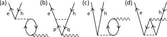
Figure 1: First-order Coulomb corrections to the amplitude for one-photon interband absorption (for noninteracting single-particle states). The final-state exciton is $(e,h)$. Upward-pointing lines indicate states in the CB, downward-pointing lines states in the VB.

In Fig. 1, we show the the first-order Coulomb correction to the interband absorption amplitude Mahan (2000); Lindgren and Morrison (1986); Shavitt and Bartlett (2009). There are four time-ordered many-body diagrams in first order, as shown in the figure. Now, in envelope-function approaches, Coulomb matrix elements in which the band index changes at one or both vertices are suppressed (they correspond to higher-order $\mathbf{k}\cdot\mathbf{p}$ corrections), and such diagrams vanish in the effective-mass limit (see, for example, Ref. Kira and Koch (2012)). One thus expects Figs. 1(a), 1(c), and 1(d) to be small, since the band index changes at both vertices of the Coulomb interaction and these diagrams are therefore formally of order $(\mathbf{k}\cdot\mathbf{p})^{2}$ or $(L_{\text{atom}}/L_{\text{dot}})^{2}$. Only Fig. 1(b) is of order $(\mathbf{k}\cdot\mathbf{p})^{0}$ and remains nonzero in the effective-mass limit. This diagram is the vertex correction to the electron-photon interaction; it forms the dominant many-body correction for an interband matrix element Mahan (2000); Elliott (1957). Note that this situation contrasts with absorption by atoms and molecules, where all four of the analogous diagrams give important correlation corrections Lindgren and Morrison (1986); Shavitt and Bartlett (2009). In this paper, we shall limit our discussion of correlation effects in semiconductor NCs to Fig. 1(b).

The vertex correction represents the interaction between the electron and hole in the final state $(e,h)$ of the absorption, and it thus accounts for the correlation in the final-state exciton wave function in Eq. (7). The same physical effect in NCs is often treated via a one-parameter variational ansatz for the exciton wave function introduced by Takagahara Takagahara (1987); Becker et al. (2018). In this paper, we will instead treat the vertex correction using the methods of MBPT, by summing over the virtual states of a HF basis set.

The first-order vertex correction, Fig. 1(b), can be analyzed using methods of degenerate (open-shell) MBPT Lindgren and Morrison (1986); Shavitt and Bartlett (2009). The expressions for the lowest- and first-order absorption amplitude (full, not reduced), in the case where the single-particle states are formed in a HF potential, are given by

$$\mathbf{M}_{eh}^{(0)} = \langle e|\mathbf{p}|h\rangle\,,$$ (13)

$$\mathbf{M}_{eh}^{(1)}(\omega) = -\sideset{}{{}^{\prime}}{\sum}_{pq}\frac{\langle eq|g_{12}|ph\rangle\langle p|\mathbf{p}|q\rangle}{\omega+\epsilon_{q}-\epsilon_{p}}\,.$$ (14)

Here, $\omega$ is the excitation frequency, $p$ are CB states, $q$ are VB states, and $\epsilon_{p}$ and $\epsilon_{q}$ are the HF eigenvalues of these states. The prime on the summation indicates that terms are to be excluded where $p$ or $q$ is a magnetic substate lying in the shells of the external legs ($p\notin e_{\text{shell}},$ $q\notin h_{\text{shell}}$). Note that the first-order absorption amplitude depends on the excitation frequency $\omega$ via the energy denominator. A similar expression for the first-order vertex correction can be applied to emission by putting $\omega=\omega_{eh}$, the energy of the emitted photon .

The corresponding expression for the reduced first-order amplitude $M_{eh}^{(1)}$ can be found by coupling the external legs of the diagram to a total angular momentum $F_{\text{tot}}$, in analogy with Eq. (11). The final result is given in Appendix B, in the form of radial integrals and angular factors.

Table 1: The first-order (vertex-corrected) reduced interband momentum matrix element for the ground-state $1S_{e}$-$1S_{h}$ ($F_{\text{tot}}=1$) exciton in a NC of CsPbBr₃ with edge length $L=11$ nm, using the material parameters in Table 2 (with $E_{P}=20$ eV). Notation: $iM^{(1)}$ is the total first-order reduced matrix element; $iM_{K}^{(1)}$ is the partial-wave contribution to $iM^{(1)}$ arising from multipole $K$ (see Appendix B); ‘extrap.’ is an estimate of the extrapolated contribution from $K=13$ to infinity. Units: atomic units. The lowest-order reduced matrix element is $iM^{(0)}=0.847$ a.u..

$K$	$iM_{K}^{(1)}$	$M_{K}^{(1)}/M^{(1)}$ (%)
0	$0.045$	$5.7$
1	$0.375$	$47.8$
2	$0.129$	$16.5$
3	$0.065$	$8.3$
4	$0.039$	$4.9$
5	$0.025$	$3.2$
6	$0.018$	$2.3$
7	$0.013$	$1.7$
8	$0.010$	$1.3$
9	$0.008$	$1.0$
10	$0.006$	$0.8$
11	$0.005$	$0.7$
12	$0.004$	$0.6$
extrap.	$0.042(4)$	$5.4$
Total $iM^{(1)}$	$0.785(4)$
$i(M^{(0)}+M^{(1)})$	$1.632(4)$

An example calculation of $M_{eh}^{(1)}$ for the ground-state $1S_{e}$-$1S_{h}$ exciton in a NC of CsPbBr₃ is given in Table 1. The total angular momentum in this case can take the values $F_{\text{tot}}=1$ (bright exciton) or $F_{\text{tot}}=0$ (dark exciton), and the matrix element shown applies to the allowed decay from $F_{\text{tot}}=1$. The first-order matrix element is expressed as a sum over contributions from Coulomb multipoles $K$, according to Eq. (30). For the $1S_{e}$-$1S_{h}$ exciton, the multipole $K$ also corresponds to the orbital angular momentum of the states $p$ and $q$ in Eq. (14). For example, for $K=1$, the states $p$ and $q$ can have all combinations of the angular momenta $P_{1/2}$ and $P_{3/2}$. The $P$-wave angular channel can be seen to dominate the sum, accounting for about 50% of the matrix element. The sum over $K$ converges quite slowly, however, with an asymptotic form approximately proportional to $1/K^{2}$; this allows us to estimate the extrapolated contribution from $K=13$ to infinity, which is about $5\%$ of the total first-order matrix element. In order to obtain an overall precision of better than 1% in the first-order matrix element, it is necessary to include the first 9 or more principal quantum numbers in the intermediate sums (at least, in the dominant $P$-wave channel).

The vertex correction in Table 1 can be seen to be a large effect for the ground-state exciton considered here. Including the first-order correction leads to a reduction in the radiative lifetime by a factor of $[(M^{(0)}+M^{(1)})/M^{(0)}]^{2}\approx 3.7$ relative to the HF value. These large vertex-renormalization factors are to be expected for a NC in intermediate confinement Takagahara (1987); Becker et al. (2018), which is the case here (see Sec. III.1). However, as we shall see in Sec. III.3, the vertex renormalization factors decrease rapidly as a function of excitation energy and approach unity for excited-state excitons.

III Results and discussion

III.1 Material parameters

Table 2: Material parameters for CsPbBr₃ and CsPbI₃ used in this work. See Sec. III.1 for explanation. $E_{P}^{(4)}$ is the Kane parameter estimated from the $4\times 4$ $\mathbf{k}\cdot\mathbf{p}$ model, and $E_{P}^{(8)}$ is estimated from the $8\times 8$ $\mathbf{k}\cdot\mathbf{p}$ model [see Eq. (15)].

	CsPbBr3	CsPbI3
$\mu^{*}$ ($m_{0}$)	$0.126$	$0.114$
$m_{e}^{*}=m_{h}^{*}$ ($m_{0}$)	$0.252$	$0.228$
$E_{g}$ (eV)	$2.342$	$1.723$
$\Delta_{\text{soc}}$ (eV)	$1.0$	$1.0$
$E_{P}^{(4)}$ (eV)	$27.9$	$22.7$
$E_{P}^{(8)}$ (eV)	$16.4$	$13.9$
$\varepsilon_{\text{eff}}$	$7.3$	$10.0$
$\varepsilon_{\text{opt}}$	$4.84$	$4.7$
$\varepsilon_{\text{out}}$	$2.4$	$2.4$

The material parameters used in this work are summarized in Table 2. We have taken the reduced mass $\mu^{*}$, the band gap $E_{g}$, and the ‘effective’ dielectric constant $\varepsilon_{\text{eff}}$ from Yang et al. Yang et al. (2017); these were measured at cryogenic temperatures for the orthorhombic phase of CsPbBr₃ and the cubic phase of CsPbI₃ Cottingham and Brutchey (2016); Stoumpos et al. (2013); Hirotsu et al. (1974). While $\mu^{*}=m_{e}^{*}m_{h}^{*}/(m_{e}^{*}+m_{h}^{*})$ is known, the individual effective masses of electron $m_{e}^{*}$ and hole $m_{h}^{*}$ are not. However, there is evidence from experiment Fu et al. (2017a) and first-principles calculations Becker et al. (2018); Protesescu et al. (2015); Umari et al. (2014) that the effective masses are approximately equal for inorganic perovskites, so we will assume $m_{e}^{*}=m_{h}^{*}$. The spin-orbit splitting $\Delta_{\text{soc}}$ between the $p_{1/2}$-like and the higher-lying $p_{3/2}$-like band is taken from Ref. Yu (2016).

The dielectric constant $\varepsilon_{\text{in}}$ used to screen the Coulomb interactions (2), for both the HF equations and the vertex correction, will be taken to be the ‘effective’ constant $\varepsilon_{\text{in}}=\varepsilon_{\text{eff}}$ measured in Ref. Yang et al. (2017). The constant $\varepsilon_{\text{eff}}$ is derived from the binding energy of the bulk exciton and therefore applies to a length scale of order the Bohr radius $a_{B}$, which is quite close to the size of the NCs that we calculate (using the parameters in Table 2, one finds $2a_{B}=6.1$ nm for CsPbBr₃ and $2a_{B}=9.3$ nm for CsPbI₃). We also need optical dielectric constants $\varepsilon_{\text{in}}^{\prime}=\varepsilon_{\text{opt}}$ to calculate the dielectric screening factor $f_{\varepsilon}$ (10). Note that the constant $\varepsilon_{\text{opt}}$ applies to a length scale given by the wavelength (we take $\lambda=500$ nm, an energy just above the threshold for absorption) and to a frequency $\omega=c/\lambda$. Inorganic perovskites present the difficulty that the bulk dielectric function varies rapidly with length and frequency scales, as can be seen from the significant difference between $\varepsilon_{\text{eff}}$ and $\varepsilon_{\text{opt}}$ in Table 2.

Also important is the Kane parameter $E_{P}$, defined by Eq. (24), which serves a dual purpose in the present work: it controls the $\mathbf{k}\cdot\mathbf{p}$ corrections via the coupling of the VB and the CB in the $4\times 4$ $\mathbf{k}\cdot\mathbf{p}$ model, and it controls the strength of the interband electron-photon interaction, where the coupling constant is proportional to $\sqrt{E_{P}}$ Mahan (2000); Elliott (1957); Efros and Efros (1982), as can be seen from Eq. (22). However, no direct measurements of $E_{P}$ exist for CsPbBr₃ or CsPbI₃. An estimate of $E_{P}$ can be made within an extended $8\times 8$ $\mathbf{k}\cdot\mathbf{p}$ model, which includes the $s$-like VB ($R_{6}^{+}$) and the $p_{1/2}$-like CB ($R_{6}^{-}$) of the $4\times 4$ model, together with the spin-orbit-split-off $p_{3/2}$-like CB band ($R_{8}^{-}$), at the $R$ point of the Brillouin zone. If one assumes that the contribution of remote bands to $m_{e}^{*}$ and $m_{h}^{*}$ is zero, this model implies

$$\frac{1}{\mu^{*}}=\frac{2}{3}\left(\frac{E_{P}}{E_{g}}+\frac{E_{P}}{E_{g}+\Delta_{\text{soc}}}\right)\,.$$ (15)

This equation can now be solved for $E_{P}$. By allowing $\Delta_{\text{soc}}\rightarrow\infty$ in Eq. (15), one obtains the corresponding equation Even et al. (2014); Yang et al. (2017) for the $4\times 4$ $\mathbf{k}\cdot\mathbf{p}$ model.

The values of $E_{P}$ inferred in this way for the $8\times 8$ and $4\times 4$ models are summarized in Table 2. We take the view that $E_{P}$ is uncertain. A conservative range would be $10\,\text{eV}\leq E_{P}\leq 32\,\text{eV}$ for CsPbBr₃ and $8\,\text{eV}\leq E_{P}\leq 26\,\text{eV}$ for CsPbI₃. We discuss this issue further in the next section.

III.2 Radiative lifetimes

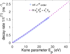
Figure 2: Bright-exciton decay rate $1/\tau$ vs. Kane parameter $E_{P}$ for NCs of CsPbBr₃ with edge length $L=9$ nm. Diamonds: calculated values (HF plus first-order vertex correction) for $E_{P}\lesssim 28$ eV; dashed line: a fit to a quadratic in $E_{P}$, $1/\tau=a_{1}^{\tau}E_{P}+a_{2}^{\tau}E_{P}^{2}$.

The radiative decay rate of the ground-state bright exciton $1S_{e}$-$1S_{h}$ ($F_{\text{tot}}=1$) in the effective-mass approximation (EMA) is proportional to the Kane parameter $E_{P}$ Efros and Efros (1982). In Fig. 2, we show the radiative decay rate of a NC of CsPbBr₃ calculated by the present methods ($\mathbf{k}\cdot\mathbf{p}$ and MBPT), for a range of values of $E_{P}$. The fit to the calculated points is indeed quite linear, although a small curvature is present owing to the higher-order $\mathbf{k}\cdot\mathbf{p}$ corrections included in the present approach. This approximate proportionality of the radiative decay rate (and also of the one-photon absorption cross section) to $E_{P}$ complicates quantitative comparisons between theory and experiment while the value of $E_{P}$ is uncertain. For illustrative purposes, in subsequent figures we shall use the values $E_{P}=20$ eV (CsPbBr₃) and $E_{P}=17$ eV (CsPbI₃), which are close to the average of $E_{P}^{(4)}$ and $E_{P}^{(8)}$ in Table 2.

Note that the calculated points in Fig. 2 are for $E_{P}\lesssim 28$ eV. For higher values of $E_{P}$, we find that the $4\times 4$ $\mathbf{k}\cdot\mathbf{p}$ model develops unphysical intragap solutions, similar to those encountered in $\mathbf{k}\cdot\mathbf{p}$ models applied to NCs of III-V and II-VI compounds Wang (2000). However, if required, it is always possible to attempt to extrapolate physical observables to values of $E_{P}\gtrsim 28$ eV, as has been done in Fig. 2.

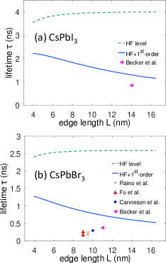
Figure 3: Bright-exciton lifetime vs. edge length $L$ for NCs of (a) CsPbI₃ ($E_{P}=17$ eV) and (b) CsPbBr₃ ($E_{P}=20$ eV). Dashed curve: HF; continuous curve: HF plus first-order vertex correction. Experimental results: Becker et al., Ref. Becker et al. (2018); Rainò et al., Ref. Rainò et al. (2016); Fu et al., Ref. Fu et al. (2017b); Canneson et al., Ref. Canneson et al. (2017).

In Fig. 3, theoretical lifetimes for NCs of CsPbI₃ and CsPbBr₃ are shown as a function of edge length $L$ and compared with available measurements. We note first that the lifetime is nearly independent of $L$ in the HF approximation, the standard result for the strong-confinement limit Efros and Efros (1982). Indeed, HF behaves like a strong-confinement theory, since the single-particle states have the quantum numbers of the strong-confinement limit and there is no correlation between electrons and holes (mean-field theory). On the other hand, the vertex correction introduces correlation, which leads to a reduction in lifetime for increasing NC size Efros and Efros (1982); Takagahara (1987), as can be observed in Fig. 3. However, we find that for large NC sizes $L\gg 2a_{B}$, the radiative lifetime varies as $\tau\sim 1/L$ using the present approach with a first-order vertex correction, instead of following the dependence $\tau\sim 1/L^{3}$ predicted by Refs. Efros and Efros (1982); Takagahara (1987). To reproduce this $1/L^{3}$ dependence within MBPT (using the same assumptions as Refs. Efros and Efros (1982); Takagahara (1987)) evidently requires an all-order treatment of the vertex correction. Nevertheless, the first-order treatment used here might be expected to be a reasonable theory in the regime of intermediate confinement, where the $L$-dependence of the lifetime interpolates the expected $1/L^{3}$ dependence of the weak-confinement limit and the $L^{0}$ dependence of the strong-confinement limit. The data in Fig. 3 are close to intermediate confinement (see Sec. III.1 for a discussion of the Bohr radius $a_{B}$).

We note also that the measurements for CsPbBr₃ in Fig. 3 show a $\pm 40$% discrepancy among themselves. They all use toluene as the surrounding medium, although in some cases (e.g., Ref. Becker et al. (2018)) there are additives. The edge length shown in the figure corresponds to the average value of $L$ for the ensemble of NCs synthesized; the size fluctuation is of order $\pm(0.5\text{--}1.0)$ nm for all the measurements. The ensemble can also be expected to contain a range of shape deformations (tetragonal, orthorhombic, and other) of the basic cubic NC shape, and possibly different crystal phases as well Cottingham and Brutchey (2016); Stoumpos et al. (2013); Hirotsu et al. (1974).

Temperature-dependent effects can also be important. The measured lifetimes are longer at room temperature Rainò et al. (2016). At the cryogenic temperatures used for the measurements in Fig. 3, the thermal occupation of the fine-structure states of the bright exciton can be nonuniform. The fine-structure splittings are typically found to be a few meV and can vary markedly from dot to dot in single-dot measurements Becker et al. (2018). The lifetime may possibly depend on the fine-structure component, depending on the origin of the splitting, and therefore on the particular NC being investigated (in single-dot measurements) and on the precise temperature of the experiment; our calculation is effectively based on the assumption of zero fine-structure splitting.

Another issue is that the measured decay rate would not be the radiative rate if there were competing nonradiative decay channels. For instance, if there were nonradiative decay channels directly from the bright state, the measured lifetimes would then be too small. However, the quantum yields are high (e.g., of order 88% for a NC of CsPbBr₂Cl measured in Ref. Becker et al. (2018)), and there is strong evidence that the bright exciton state is the ground state in CsPbBr₃ Becker et al. (2018), so that nonradiative decay channels from the bright state seem likely to be suppressed.

We see from Fig. 3 that inclusion of the vertex correction markedly improves agreement between theory and experiment. Nevertheless, the final MBPT values of the lifetime, for the illustrative values of the Kane parameter chosen [$E_{P}=20$ eV (CsPbBr₃) and $E_{P}=17$ eV (CsPbBr₃)], still globally overestimate the measured values, both for CsPbBr₃ and for CsPbI₃. A simple approach would be to fit $E_{P}$ to the experiments; this would require values of $E_{P}$ somewhat in excess of the value $E_{P}^{(4)}$ in Table 2 inferred from the $4\times 4$ $\mathbf{k}\cdot\mathbf{p}$ model. However, we note that there are other sources of theoretical uncertainty, besides the Kane parameter. The main ones are:

(i) Uncertainty in dielectric constants. The optical dielectric constant $\varepsilon_{\text{in}}^{\prime}=\varepsilon_{\text{opt}}$ varies rapidly in the vicinity of the absorption threshold Dirin et al. (2016); Singh et al. (2019) and this influences the lifetime through the dielectric screening factor $f_{\varepsilon}$ (10); the values used here (Table 2) correspond to a wavelength $\lambda=500$ nm. Also, the dielectric constant of the surrounding medium would vary if there are additives Becker et al. (2018); we have here assumed the value for pure toluene. As an example of the possible effect of these uncertainties, we note that a 15% uncertainty in $\varepsilon_{\text{opt}}$ and a 5% uncertainty in $\varepsilon_{\text{out}}$ would lead to about a 17% uncertainty in the lifetime.

In addition, the vertex-renormalization factor is sensitive to the dielectric constant $\varepsilon_{\text{in}}$ used to screen the Coulomb interactions (2), since the first-order Coulomb correction is proportional to $1/\varepsilon_{\text{in}}$. We have assumed $\varepsilon_{\text{in}}=\varepsilon_{\text{eff}}$ in our calculations (see Sec. III.1). But the length scale for the NCs is not identical to that of the bulk exciton from which the constant $\varepsilon_{\text{eff}}$ was inferred, and the vertex correction also samples parts of the bulk dielectric function at nonzero frequency Mahan (2000), so the appropriate value of $\varepsilon_{\text{in}}$ might be somewhat different from $\varepsilon_{\text{eff}}$. As mentioned in Sec. III.1, the bulk dielectric function varies rapidly with distance and frequency. This issue is hard to quantify, but as an example, if we assume that $\varepsilon_{\text{in}}$ is 15% smaller than $\varepsilon_{\text{eff}}$, then the vertex renormalization factor would increase, and the lifetime would decrease, also by about 15%.

We note that we have also neglected the effect of the dielectric mismatch between the NC and the surrounding medium Karpulevich et al. (2019), and that boundary effects can be further modified by the ligands Karpulevich et al. (2019).

(ii) Corrections for cubic NCs. Although the perovskite NCs in this study are generally cuboid, we have assumed a spherical NC with an effective radius given by Eq. (4). As mentioned in Sec. II.1, many errors from this approximation are expected to enter at the few percent level for the ground-state exciton. One source of error that we did not discuss in Sec. II.1 concerns the value of the dielectric screening factor $f_{\varepsilon}$. The calculations above have assumed the spherical value $f_{\varepsilon}^{\text{sph}}$ (10). However, according to the numerical calculations for a cube in Ref. Becker et al. (2018), for the case of intermediate confinement with $\varepsilon_{\text{in}}^{\prime}/\varepsilon_{\text{out}}\approx 2$ (as in Table 2), the ratio of lifetimes for a cubic NC and a spherical NC with the same volume is $\tau^{\text{cube}}/\tau^{\text{sph}}\approx 1.4$. If instead of equal volumes we use a sphere radius given by Eq. (4) and assume that the lifetime is approximately inversely proportional to the volume, then the ratio calculated in Ref. Becker et al. (2018) is modified to $\tau^{\text{cube}}/\tau^{\text{sph}}\approx 1.12$. Thus, according to these estimates, our theoretical values for the lifetime in Fig. 3 should be increased by about 12%. These results also imply that $f_{\varepsilon}^{\text{sph}}/f_{\varepsilon}^{\text{cube}}\approx 1.06$ for the parameters used here. Another calculation gives $f_{\varepsilon}^{\text{sph}}/f_{\varepsilon}^{\text{cube}}\approx 0.99$ for $\varepsilon_{\text{in}}^{\prime}/\varepsilon_{\text{out}}\approx 2$ in the strong-confinement limit .

(iii) Higher-order MBPT. We use a first-order vertex correction. Unfortunately, it is difficult to estimate the effect of the omitted higher-order vertex terms without explicit calculation. Comparing with the results of the variational calculation in Ref. Becker et al. (2018), however, we conclude that the ground-state vertex renormalization factors (for intermediate confinement) could be increased by as much as 40% beyond their first-order value.

We believe that the present discrepancy between theory and experiment is due to a combination of (iii) above and our use of the wrong value of the Kane parameter, with further contributions from the other sources of uncertainty (including experimental).

III.3 One-photon absorption spectra

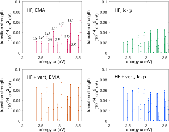
Figure 4: Transition strengths, Eq. (16), in various approximations for a NC of CsPbBr₃ with edge length $L=9$ nm ($E_{P}=20$ eV). The energy axis gives the exciton energy $\omega_{eh}=\epsilon_{e}-\epsilon_{h}$ for each possible final-state exciton $(e,h)$. Notation: EMA, effective-mass approximation; $\mathbf{k}\cdot\mathbf{p}$, $4\times 4$ $\mathbf{k}\cdot\mathbf{p}$ model; HF, Hartree-Fock; HF + vert, Hartree-Fock plus first-order vertex correction. Two levels of many-body theory are considered: HF (upper panels) and HF with first-order vertex correction (lower panels). For each, we employ either the EMA (left panels) or the full $4\times 4$ $\mathbf{k}\cdot\mathbf{p}$ model (right panels). In the top-left panel, the first few exciton state assignments are shown: “$1S$” indicates a $1S_{e}$-$1S_{h}$ exciton, “$1P$” a $1P_{e}$-$1P_{h}$ exciton, “$2S$” a $2S_{e}$-$2S_{h}$ exciton, etc. The corresponding transitions in the other three panels have the same state assignments.

In this paper, we will only consider absorption from the highest-lying VB ($R_{6}^{+}$) to the lowest-lying CB ($R_{6}^{-}$), around the $R$ point of the Brillouin zone. A study of bulk excitons at cryogenic temperatures in (CH₃NH₃)PbBr₃ Tanaka et al. (2003), which may be expected to have a band structure similar to that of CsPbBr₃, showed a sharp excited line at 3.3 eV, which was attributed to transitions from the $s$-like VB ($R_{6}^{+}$) to the $p_{3/2}$-like spin-orbit-split-off CB ($R_{8}^{-}$); there were also higher-lying structures around 3.9 eV, attributed to interband transitions at the $M$ point. Absorption spectra of NCs of CsPbBr₃ often show corresponding features (see, for example, Refs. Chen et al. (2017a); Brennan et al. (2017)). In particular, a step in the absorption spectrum is often visible around 3.0–3.2 eV (for edge lengths $L\sim 9$ nm), which likely corresponds to the transition $R_{6}^{+}\rightarrow R_{8}^{-}$, in analogy with bulk (CH₃NH₃)PbBr₃. This identification is consistent also with density-functional (DFT) band-structure calculations in CsPbBr₃ Becker et al. (2018). Because we focus on the $R_{6}^{+}\rightarrow R_{6}^{-}$ transition here, the range of validity of our results will extend from the absorption threshold at about 2.35 eV up to about 3.1 eV.

The first step in the calculation of the one-photon absorption cross section (8) is to calculate the reduced matrix elements $M_{eh}$ for a large set of transitions to all possible final-state excitons $(e,h)$ (with $F_{\text{tot}}=1$). We define the transition strength $T_{eh}(\omega)$ for a particular final state $(e,h)$ to be the coefficient of the line-shape function $\Delta_{eh}(\omega-\omega_{eh})$ in Eq. (8),

$$T_{eh}(\omega)=\frac{4\pi^{2}}{3}\frac{f_{\varepsilon}^{2}}{n_{\text{out}}c\omega}\left|M_{eh}\right|^{2}\,.$$ (16)

Transition strengths $T_{eh}(\omega_{eh})$ are shown in Fig. 4 in various approximations. In the EMA and at HF level (top-left figure), the dominant transitions correspond to excitons with quantum numbers $(nl)_{e}$-$(nl)_{h}$, in which both the principal quantum number $n$ and the orbital angular momentum $l$ of the electron and hole are equal. Thus, the lowest-energy transition in the figure is the $1S_{e}$-$1S_{h}$ exciton discussed in the previous section, the next group corresponds to $1P_{e}$-$1P_{h}$ (with various $F$-dependent fine-structure components), and so on. The selection rule on $l$ here follows directly from Eq. (22); the approximate selection rule on $n$ follows because corresponding electron and hole wave functions are approximately equal, so that terms with $n_{e}\neq n_{h}$ are highly suppressed by the near orthogonality of the radial functions in Eq. (22).

When the HF calculation is repeated within the $4\times 4$ $\mathbf{k}\cdot\mathbf{p}$ model (top-right panel of Fig. 4), one observes a small overall reduction in transition strength, accompanied by an increase in the density of exciton final states. Also, the non-$S$-wave states develop a ‘fine structure’ corresponding to the different possible values of total angular momentum $F$, Eq. (5). Thus, a $1P_{e}$-$1P_{h}$ exciton is split into $(1P_{1/2})_{e}$-$(1P_{1/2})_{h}$, $(1P_{1/2})_{e}$-$(1P_{3/2})_{h}$, $(1P_{3/2})_{e}$-$(1P_{1/2})_{h}$, and $(1P_{3/2})_{e}$-$(1P_{3/2})_{h}$ components with small energy splittings. The fine structure is more visible for higher excited excitons such as $1H_{e}$-$1H_{h}$. Moreover, new transitions appear with low transition strength. This happens because the $\mathbf{k}\cdot\mathbf{p}$ corrections allow nonzero matrix elements such as $\langle(1S_{1/2})_{e}|\mathbf{p}|(1D_{3/2})_{h}\rangle$ via the ‘small-small’ terms of Eq. (22) and the ‘large-small’ terms of Eq. (25). In the EMA, this matrix element would be forbidden because $l_{e}\neq l_{h}$.

In the lower panels of Fig. 4, we apply the first-order vertex correction (14) to all the transitions calculated in the upper panels . The vertex correction can be seen to enhance the transition strength of the corresponding transition in the upper panel, as discussed for the ground-state $1S_{e}$-$1S_{h}$ exciton in the previous section. However, while the enhancement factor is large (around 3.5–4) for the ground-state exciton, inspection of the dominant transitions in Fig. 4 reveals that the enhancement factor decreases rapidly with increasing energy, so that near $\omega_{eh}=3.1$ eV, it is much closer to unity, around 1.4, while for $\omega_{eh}=3.6$ eV, it has decreased further to about 1.1. A simple way to understand this result is to reflect that the Bohr radius of excited states is larger, so that excited-state excitons are more strongly confined than the ground-state exciton, for a given NC size.

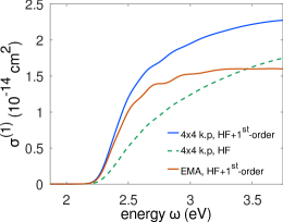
Figure 5: Calculated one-photon absorption cross section for a NC of CsPbBr₃ with edge length $L=9$ nm ($E_{P}=20$ eV) in various approximations. Notation: HF, Hartree-Fock; EMA, effective-mass approximation; 1st-order, first-order vertex correction.

In the next step of the calculation, we assign line-shape functions $\Delta_{eh}(\omega-\omega_{eh})$ to each transition to produce a broadened absorption spectrum according to Eq. (8). In principle, the function $\Delta_{eh}(\omega-\omega_{eh})$ is a Lorentzian for intrinsic dephasing mechanisms (homogeneous broadening), and it is also necessary to average physical observables over the parameters of the ensemble (inhomogeneous broadening) Hu et al. (1990, 1996). Here we will adopt a simpler, phenomenological approach emphasizing inhomogeneous broadening. An important source of inhomogeneous broadening is by the distribution of sizes in the NC ensemble. For NCs of CsPbBr₃, the measured histogram of edge lengths $L$ can be fitted to a normal distribution, yielding a standard deviation $\delta L$ with typical values varying from $\delta L/L\approx 5$% Chen et al. (2017a); Brennan et al. (2017) to about 10% Makarov et al. (2016); Nagamine et al. (2018). Now, since the confinement energy is approximately proportional to $1/L^{2}$ and the Coulomb energy to $1/L$, the exciton energy can be approximately parametrized as

$$\omega_{eh}(L)=E_{g}+\frac{A_{eh}}{L^{2}}+\frac{B_{eh}}{L}\,.$$ (17)

This equation, with values of $A_{eh}$ and $B_{eh}$ extracted from the HF spectrum, may be used to relate the width $\sigma_{eh}^{\text{size}}$ of the distribution of energies $\omega_{eh}$ to the width $\delta L$ of the distribution of edge lengths $L$. The width $\sigma_{eh}^{\text{size}}$ calculated in this way is found to increase as the exciton energy $\omega_{eh}$ increases. We then take the line-shape function to be a Gaussian

$$\Delta_{eh}(\omega-\omega_{eh})=\frac{1}{\sigma_{eh}\sqrt{2\pi}}\exp\left[-\frac{(\omega-\omega_{eh})^{2}}{2\sigma_{eh}^{2}}\right]\,,$$ (18)

with $\sigma_{eh}=\sigma_{eh}^{\text{size}}$.

However, we find that size broadening alone, assuming $\delta L/L=5$–10%, typically produces insufficiently broadened absorption spectra containing sharp subpeaks, which are generally not observed in measured absorption spectra of NCs of CsPbBr₃ Wang et al. (2015); Makarov et al. (2016); Xu et al. (2016); Chen et al. (2017a); Brennan et al. (2017); Nagamine et al. (2018). Therefore, we need to consider other broadening mechanisms. These include phonon broadening Gammon et al. (1996) and the distribution of NC shape deformations present in the ensemble. We will treat these effects purely phenomenologically by introducing a second width $\sigma^{\text{other}}$, which we take to be a constant for all excitons $(e,h)$. The total Gaussian width in Eq. (18) is then given by

$$\sigma_{eh}^{2}=\left(\sigma_{eh}^{\text{size}}\right)^{2}+\left(\sigma^{\text{other}}\right)^{2}\,.$$ (19)

(Note that we here approximate the effect of the homogeneous phonon broadening with a Gaussian.) A reasonable fit to the appearance of the measured spectra can now be obtained by, for example, taking $\sigma^{\text{other}}\approx 60$ meV and $\delta L/L\approx 5$%.

One-photon absorption spectra broadened in this way are shown in various approximations in Fig. 5. The theoretical spectra can be understood in terms of the underlying transition strengths in Fig. 4, discussed above. After line-shape broadening, the net effect of the $\mathbf{k}\cdot\mathbf{p}$ corrections is found to be a surprisingly large increase in the calculated cross section, reaching about 30% at $\omega=3.1$ eV. The cross section is also enhanced by the vertex correction, although the enhancement factor is seen to be much greater near the threshold than at higher energies, having a value of only about 1.4 for the broadened cross section at $\omega=3.1$ eV.

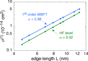
Figure 6: Log-log plot of the theoretical one-photon absorption cross section at $\omega=3.1$ eV vs. edge length $L$ for a NC of CsPbBr₃ ($E_{P}=20$ eV). Circles/Diamonds: calculated points. Lines: fitted power-law dependence $\sigma^{(1)}(\omega)\propto L^{\alpha}$, with the exponent $\alpha$ given by the slope of a straight-line fit in logarithmic space.

In Fig. 6, we show a log-log plot of the calculated $\sigma^{(1)}(\omega)$ as a function of edge length $L$ at an energy $\omega=3.1$ eV. The linearity of the log-log plot demonstrates that the theoretical cross section for this energy fits well a power-law dependence $\sigma^{(1)}(\omega)\propto L^{\alpha}$. A least-squares fit to the MBPT calculation over the size range $4.5\,\text{nm}\leq L\leq 12.5\,\text{nm}$ (Fig. 6) yields a theoretical exponent $\alpha=2.88$. This exponent agrees well with a fit to the one-photon experimental data of Chen et al. Chen et al. (2017a) over the same size range and at the same energy, which follow closely a power law with an exponent $\alpha_{\text{expt}}=2.9\pm 0.2$.

One $L$-dependent term in the theory that contributes to this exponent is the vertex renormalization factor. We have seen, however, that at an energy of $\omega=3.1$ eV, the vertex renormalization factor for transition strengths is quite close to unity, of order 1.4 (Fig. 4), and as a result its $L$-dependence can be expected to be a rather weak effect. Indeed, a fit to the HF cross section (no vertex correction present) yields a theoretical exponent $\alpha=3.02$, implying that the vertex correction modifies the exponent by roughly $\delta\alpha_{\text{vert}}\approx-0.14$. We conclude that the dominant $L$-dependent term is the density of final-state excitons. In 3D, the density of states is proportional to the volume of the confining box Mahan (2000), at least in the limit of large volumes. Although the transitions (Fig. 4) are still quite discrete at an energy of $\omega=3.1$ eV, the line-shape broadening discussed above yields an average density of states at that energy. The final theoretical exponent is indeed very close to 3, particularly at HF level.

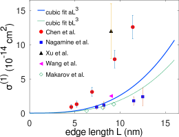
Figure 7: One-photon absorption cross section at $\omega=3.1$ eV vs. edge length $L$ for a NC of CsPbBr₃. Full curves: theoretical curves ($E_{P}=20$ eV) at HF level (lower curve) and using HF plus the first-order vertex correction (upper curve), taken from Fig. 6. Circles/diamonds/triangles/squares: experimental points. Chen et al., Ref. Chen et al. (2017a); Nagamine et al., Ref. Nagamine et al. (2018); Xu et al., Ref. Xu et al. (2016); Wang et al., Ref. Wang et al. (2015); Makarov et al., Ref. Makarov et al. (2016).

In Fig. 7, we compare our theoretical cross section at $\omega=3.1$ eV with the results of the available experiments that report absolute (normalized) cross sections. It can be seen that there is significant disagreement between the various measurements, which is probably due to uncertainties in the procedure for normalizing the experimental cross section. The theoretical result (for $E_{P}=20$ eV) is intermediate among the various measurements. The contributions to theoretical uncertainty discussed in Sec. III.2 for the lifetime apply here also, except that at an energy of $\omega=3.1$ eV, the uncertainty due to omitted higher-order MBPT is much less, because the vertex renormalization factors are close to unity (about 1.4), and as a result, the calculation of the vertex factor can be expected to be quite perturbative. Two additional error terms arise in this case, however. First, the energy $\omega=3.1$ eV chosen for the measurements (e.g., in Ref. Chen et al. (2017a)) is close to the threshold for the $R_{6}^{+}\rightarrow R_{8}^{-}$ band transition, which we have not included in our calculations. This threshold produces a step in the cross section, which increases its value by about 20–40% compared to its value on the low-energy side of the step Chen et al. (2017a).

The second error term is due to the the spherical approximation. While we pointed out in Sec. II.1 that the spectra of $S$- and $P$-like states in a cube agree well with those in the equivalent sphere (4), the absorption cross section for $\omega\approx 3.1$ eV brings in also states of higher angular momentum, up to $G$-wave and beyond (see Fig. 4). For orbital angular momenta $l\geq 2$, an $nl$ level in a sphere with degeneracy $(2l+1)$ will in general be fragmented into two or more levels in a cube, in analogy with crystal-field theory Callaway (1991). Moreover, these higher angular-momentum levels will in general be mixed by the cubic perturbation. To estimate the overall effect of the cubic corrections, we recalculated the absorption cross section at the level of noninteracting particles for both a cube and a sphere, finding that $\sigma^{(1)}(\omega)$ at $\omega=3.1$ eV for a cube is greater than that for a sphere by about 10–20% (the precise figure being sensitive to the line-shape function assumed).

The largest theoretical uncertainty at present is, however, in the value of the Kane parameter $E_{P}$, to which the theoretical cross section is approximately proportional (see Fig. 8).

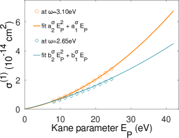
Figure 8: Calculated one-photon absorption cross section at $\omega=3.1$ eV (circles) and $\omega=2.65$ eV (diamonds) vs. Kane parameter $E_{P}$ for a NC of CsPbBr₃ with edge length $L=9$ nm. The full curves represent fits of a quadratic function of $E_{P}$ through the calculated points.

IV Conclusions

We have calculated one-photon absorption cross sections for NCs of CsPbBr₃ in various approximations, from the threshold up to an energy of about $\omega=3.1$ eV, and compared with the available measurements. The formalism used was a $4\times 4$ $\mathbf{k}\cdot\mathbf{p}$ envelope-function model, combined with a treatment of the electron-hole correlation within MBPT. In lowest order we used a HF model, to which we added the first-order vertex correction to the electron-photon interaction, which is the leading correlation correction for an interband transition. The vertex correction gives a large enhancement, by a factor of order 3.5–4, to the absorption rate for the ground-state $1S_{e}$-$1S_{h}$ exciton, but this enhancement factor is found to decrease rapidly as a function of excitation energy, so that for $E=3.1$ eV (about 0.7 eV above the absorption threshold), the enhancement factor is much closer to unity, around 1.4.

The one-photon absorption cross section was obtained by computing the transition rates to all relevant final-state excitons, with each transition broadened phenomenologically by considering the distribution of NC sizes in the ensemble (among other broadening mechanisms). We gave a theoretical discussion of the absorption cross section in various approximations, emphasizing the above-mentioned energy-dependent enhancement by the vertex correction, as well as the effect of the $\mathbf{k}\cdot\mathbf{p}$ corrections, which turned out to be surprisingly large, yielding a 30% enhancement of the cross section at $E=3.1$ eV relative to a treatment within the effective-mass approximation. The theoretical absorption cross section at $E=3.1$ eV was shown to follow closely a power-law dependence $\sigma^{(1)}(\omega)\propto L^{2.9}$ on the NC edge length $L$, in close agreement with the experiment of Chen et al. Chen et al. (2017a), who found an exponent $\alpha_{\text{expt}}=2.9\pm 0.2$. We attributed this power-law dependence mainly to the density of final-state excitons, with only a small contribution arising from the $L$-dependence of the vertex-correction factors.

The available experimental data for the absolute (normalized) cross section at $\omega=3.1$ eV show substantial disagreements among themselves by nearly an order of magnitude; our theoretical values (for a Kane parameter $E_{P}=20$ eV) are intermediate among the measured values. We also calculated radiative lifetimes for NCs of CsPbBr₃ and CsPbI₃, where the experimental results show a scatter of about $\pm 40$%. Our theoretical predictions of radiative lifetimes globally overestimate the experimental values by a factor of up to about two (assuming $E_{P}=20$ eV for CsPbBr₃ and 17 eV for CsPbI₃).

The theoretical approach in this work can be improved in various ways. Particularly for the radiative lifetime of the ground-state exciton, where the first-order vertex renormalization factors are large (around 3.5–4.0), an all-order calculation of the vertex correction is clearly indicated, even for the case of intermediate confinement encountered in NCs of CsPbBr₃ and CsPbI₃, and should go some way toward reducing the discrepancy with experiment observed in Fig. 3. This involves summing numerically to all orders the electron-hole Coulomb ladder diagrams for the final-state exciton Mahan (2000). Such an all-order summation is less important, however, for the one-photon absorption cross section at an energy $\omega=3.1$ eV, where the corresponding vertex factors are closer to unity (around 1.4) and the vertex correction is already quite perturbative. It would also be interesting to improve upon the spherical NC approximation used in this work, by adding nonspherical perturbations to the model to take account of the cuboid NCs found for metal-halide perovskites. Some work along these lines has been carried out in Ref. Sercel et al. (2019b).

The leading source of theoretical uncertainty at present remains the uncertain value of the Kane parameter $E_{P}$. First-principles atomistic calculations for the bulk materials should be able to help here. A DFT calculation for CsPbBr₃ Becker et al. (2018) found a reduced mass $\mu^{*}=0.065$, which is close to the result of another DFT calculation Protesescu et al. (2015), but about one half the measured reduced mass given in Table 2. The same calculation Becker et al. (2018) found $E_{P}=40$ eV, which seems too high (at least, compared to the estimates in Table 2). Further first-principles atomistic work is required to understand the origin of these discrepancies, which may imply, for example, significant phonon contributions to the material parameters.

Appendix A Reduced momentum matrix element

In this appendix, we derive an expression for the reduced momentum matrix element $\langle F_{a}\|\,p^{1}\|F_{b}\rangle$ for the $4\times 4$ $\mathbf{k}\cdot\mathbf{p}$ model for states of spherical form (5). It is convenient for this purpose to rewrite the two-component state (5) in a generalized form,

$$|\eta F_{a}m_{a}\rangle=\sum_{\alpha=1}^{2}\frac{1}{r}R_{a\alpha}(r)|(l_{a\alpha},J_{\alpha})F_{a}m_{a}\rangle\,,$$ (20)

where $\alpha=1$ or 2 denotes the component. We conventionally take $\alpha=1$ ($\alpha=2$) to refer to the component lying in the CB (VB). The radial function for component $\alpha$ is $R_{a\alpha}(r)$ and both components have Bloch angular momentum $J_{\alpha}=1/2$.

The matrix element $\langle a|\mathbf{p}|b\rangle$ is given by a sum over all combinations of the component $\alpha$ of $|a\rangle$ and the component $\beta$ of $|b\rangle$,

$$\langle F_{a}\|\,p^{1}\|F_{b}\rangle=\sum_{\alpha\beta=1}^{2}\langle F_{a},\alpha\|\,p^{1}\|F_{b},\beta\rangle\,.$$ (21)

There are two distinct cases for $\langle F_{a},\alpha\|\,p^{1}\|F_{b},\beta\rangle$. The first is when $\alpha\neq\beta$ (thus, $\alpha=1$ and $\beta=2$, or $\alpha=2$ and $\beta=1$). Here, terms where $\mathbf{p}$ acts on the envelope functions vanish, on account of the orthogonality of the Bloch functions of the CB and VB, and therefore we only need consider terms where $\mathbf{p}$ acts on the Bloch functions. Using standard methods of angular-momentum theory Lindgren and Morrison (1986); Brink and Satchler (1994), we then find

$$\langle F_{a},\alpha\|\,p^{1}\|F_{b},\beta\rangle_{\alpha\neq\beta}=$$

$$\quad\quad(-1)^{1+F_{a}+J_{\beta}+l_{a\alpha}}\delta(l_{a\alpha},l_{b\beta})$$

$$\quad\quad\times\sqrt{(2F_{a}+1)(2F_{b}+1)}\left\{\begin{matrix}F_{b}&J_{\beta}&l_{a\alpha}\\ J_{\alpha}&F_{a}&1\end{matrix}\right\}$$

$$\quad\quad\times\langle J_{\alpha}\|\,p^{1}\|J_{\beta}\rangle\int_{0}^{\infty}\!R_{a\alpha}(r)R_{b\beta}(r)\,dr\,.$$ (22)

The reduced matrix element of $p^{1}$ between Bloch states has the value

$$\langle J_{\alpha}\|\,p^{1}\|J_{\beta}\rangle=-i\sqrt{E_{P}}(-1)^{L_{\alpha}}\,,$$ (23)

where $L_{\alpha}$ is the orbital Bloch angular momentum of the band for component $\alpha$. In lead-halide perovskites, the VB is $s$-like and the CB is $p_{1/2}$-like, so $L_{1}=1$ and $L_{2}=0$. We define the Kane parameter $E_{P}$ by

$$E_{P}=2|\langle S|p_{z}|Z\rangle|^{2}\,,$$ (24)

where $|S\rangle$ is the (spin-uncoupled) Bloch state of the $s$-like band and $|Z\rangle$ is the $z$-component of the (spin-uncoupled) Bloch state of the $p$-like band .

The second case arising in Eq. (21) is when $\alpha=\beta$ (thus, $\alpha=\beta=1$ or $\alpha=\beta=2$). In this case, terms where $\mathbf{p}$ acts on Bloch functions vanish, because we are assuming the bands to have exact inversion symmetry. Therefore, we only need consider terms where $\mathbf{p}$ acts on the envelope functions. This gives

$$\langle F_{a},\alpha\|\,p^{1}\|F_{b},\beta\rangle_{\alpha=\beta}=$$

$$\quad\quad\quad(-1)^{1+F_{b}+J_{\alpha}+l_{a\alpha}}\left(\frac{1}{m_{\alpha}^{*}}\right)^{\prime}$$

$$\quad\quad\quad\times\sqrt{(2F_{a}+1)(2F_{b}+1)}\left\{\begin{matrix}F_{b}&l_{b\beta}&J_{\alpha}\\ l_{a\alpha}&F_{a}&1\end{matrix}\right\}$$

$$\quad\quad\quad\times(-i)\langle l_{a\alpha}\|\,\nabla^{1}\|l_{b\beta}\rangle\,,$$ (25)

where the reduced matrix element of the gradient operator between envelope functions is given by

$$\langle l_{a\alpha}\|\,\nabla^{1}\|l_{b\beta}\rangle=\sqrt{l_{b\beta}+1}$$

$$\quad\quad\quad\times\int_{0}^{\infty}\!R_{a\alpha}(r)\left[\frac{dR_{b\beta}(r)}{dr}-(l_{b\beta}+1)\frac{R_{b\beta}(r)}{r}\right]\,dr$$ (26)

when $l_{a\alpha}=l_{b\beta}+1$, and by

$$\langle l_{a\alpha}\|\,\nabla^{1}\|l_{b\beta}\rangle=-\sqrt{l_{b\beta}}$$

$$\quad\quad\quad\times\int_{0}^{\infty}\!R_{a\alpha}(r)\left[\frac{dR_{b\beta}(r)}{dr}+l_{b\beta}\frac{R_{b\beta}(r)}{r}\right]\,dr$$ (27)

when $l_{a\alpha}=l_{b\beta}-1$, and $\langle l_{a\alpha}\|\,\nabla^{1}\|l_{b\beta}\rangle$ is zero in all other cases.

Equation (25) contains an extra complication, the reduced-mass factor. It is well known (see, for example, Ref. Kira and Koch (2012)) that in an effective-mass model, with the VB and CB uncoupled, the inclusion of $\mathbf{k}\cdot\mathbf{p}$ corrections leads to an extra factor of $(1/m_{\alpha}^{*})$ multiplying the intraband momentum matrix element, where $m_{\alpha}^{*}$ is the band effective mass. This factor is in general large for a semiconductor (e.g., it has the value $1/m_{\alpha}^{*}\approx 4$ for CsPbBr₃ and CsPbI₃) and can not normally be neglected. An analogous argument applies to the case $\alpha=\beta$ above, except that in our coupled VB-CB model, the contributions to the effective masses arising from the VB-CB coupling are included automatically in the formalism. Therefore, we require instead a modified factor $(1/m_{\alpha}^{*})^{\prime}$ that includes only the contributions of the remote bands and the bare electron mass. In the $4\times 4$ $\mathbf{k}\cdot\mathbf{p}$ model, this modified factor for the CB ($\alpha=1)$ is given by Efros and Rosen (2000)

$$\left(\frac{1}{m_{1}^{*}}\right)^{\prime}=\frac{1}{m_{e}^{*}}-\frac{E_{P}}{3E_{g}}\,,$$ (28)

while for the VB ($\alpha=2$)

$$\left(\frac{1}{m_{2}^{*}}\right)^{\prime}=-\left(\frac{1}{m_{h}^{*}}-\frac{E_{P}}{3E_{g}}\right)\,,$$ (29)

where $m_{e}^{*}$ and $m_{h}^{*}$ are the full electron and hole effective masses, respectively (which are conventionally defined to be positive). Note that we have included an overall minus sign in the definition of $(1/m_{2}^{*})^{\prime}$ for the VB in Eq. (29); this is needed because the matrix element in Eq. (25) is defined to apply to electron states $a$ and $b$, even when the states lie in the VB. It is now possible to show, analytically or numerically, that the definitions (28) and (29), together with the matrix elements (22) and (25), imply that in the uncoupled model one recovers the standard factor $(1/m_{\alpha}^{*})$ for the intraband momentum matrix element.

Equations (21), (22), and (25) define the complete reduced matrix element. In this paper we only need interband matrix elements, but we emphasize that the same equations apply to both interband and intraband matrix elements, although different terms dominate in each case. For instance, consider an interband matrix element $\langle a|\mathbf{p}|b\rangle$, where $a$ is a CB state and $b$ is a VB state. Then, component 1 of $|a\rangle$ is the large component, and component 2 is the small component; for $|b\rangle$, the large and small components are reversed. It follows that the large-large ($\alpha=1$, $\beta=2$) term of Eq. (22) is the dominant term, while the small-small ($\alpha=2$, $\beta=1$) term is an $O(\mathbf{k}\cdot\mathbf{p})^{2}$ correction, and all the large-small terms of Eq. (25) are $O(\mathbf{k}\cdot\mathbf{p})$ corrections.

On the other hand, consider an intraband matrix element $\langle a|\mathbf{p}|b\rangle$, where both $a$ and $b$ are states in the CB. Now the dominant term is the large-large ($\alpha=1$, $\beta=1$) term from Eq. (25), while the small-small ($\alpha=2$, $\beta=2$) terms are $O(\mathbf{k}\cdot\mathbf{p})^{2}$ corrections, and all the large-small terms from Eq. (22) are $O(\mathbf{k}\cdot\mathbf{p})$ corrections.

Appendix B Angular reduction of vertex correction

To perform the angular reduction of the vertex correction, we couple the final-state exciton $(e,h)$ in Eq. (14) to a total angular momentum $F_{\text{tot}}$, as was done for the lowest-order amplitude in Eq. (11), and then perform the sums over the magnetic substates analytically Lindgren and Morrison (1986); Brink and Satchler (1994). This gives

$$M_{eh}^{(1)}(\omega) = \delta(F_{\text{tot}},1)\sideset{}{{}^{\prime}}{\sum}_{pq}\sum_{K=0}^{\infty}(-1)^{F_{p}+F_{q}}\left\{\begin{matrix}K&F_{p}&F_{e}\\ 1&F_{h}&F_{q}\end{matrix}\right\}$$ (30)

$$\quad\quad\quad\quad\quad\quad\times\frac{X_{K}(eqph)\langle p\|\,p^{1}\|q\rangle}{\omega+\epsilon_{q}-\epsilon_{p}}\,,$$

where $\langle p\|\,p^{1}\|q\rangle$ is the reduced single-particle momentum matrix element discussed in Appendix A, and $X_{K}(eqph)$ is a reduced two-body Coulomb matrix element with multipole $K$, which is defined by

$$\langle ab|g_{12}|cd\rangle=\sum_{K=0}^{\infty}\sum_{M=-K}^{K}(-1)^{F_{a}+F_{b}+K-m_{a}-m_{b}-M}\\ \quad\times\left(\begin{matrix}F_{a}&K&F_{c}\\ -m_{a}&M&m_{c}\end{matrix}\right)\left(\begin{matrix}F_{b}&K&F_{d}\\ -m_{b}&-M&m_{d}\end{matrix}\right)X_{K}(abcd)\,.$$ (31)

In the approximation that one neglects the small components of the states, the expression for $X_{K}(abcd)$ is analogous to the standard expression for an atom Lindgren and Morrison (1986),

$$X_{K}(abcd)=\frac{(-1)^{K}}{\varepsilon_{\text{in}}}\langle\kappa_{a}\|\,C^{K}\|\kappa_{c}\rangle\langle\kappa_{b}\|\,C^{K}\|\kappa_{d}\rangle$$

$$\quad\quad\times\int_{0}^{\infty}\!\int_{0}^{\infty}\!\left(R_{a}R_{c}\right)_{r_{1}}\left(R_{b}R_{d}\right)_{r_{2}}\frac{r_{<}^{K}}{r_{>}^{K+1}}\,dr_{1}dr_{2}\,.$$ (32)

Here $R_{m}(r)$ is the radial function of the large component of state $m$, and $\langle\kappa_{a}\|\,C^{K}\|\kappa_{c}\rangle$ is a reduced matrix element of the $C^{K}$ tensor between coupled spinors Edmonds (1960)

$$\langle\kappa_{a}\|\,C^{K}\|\kappa_{c}\rangle=\langle(l_{a},1/2)F_{a}\|\,C^{K}\|(l_{c},1/2)F_{c}\rangle\,.$$ (33)

$X_{K}(abcd)$ can also be generalized to include both large and small components by exploiting the analogy between the $4\times 4$ $\mathbf{k}\cdot\mathbf{p}$ model and the Dirac equation and using the techniques described in, for example, Ref. Johnson et al. (1988). We have included the small components in the numerical calculations in this paper.

In practice, the allowed multipoles of $X_{K}(abcd)$ are limited by parity and angular-momentum selection rules.

References

- Protesescu et al. (2015) L. Protesescu, S. Yakunin, M. I. Bodnarchuk, F. Krieg, R. Caputo, C. H. Hendon, R. X. Yang, A. Walsh, and M. V. Kovalenko, Nanocrystals of cesium lead halide perovskites (CsPbX3, X = Cl, Br, and I): Novel optoelectronic materials showing bright emission with wide color gamut, Nano Lett. 15, 3692 (2015).
- Krieg et al. (2018) F. Krieg, S. T. Ochsenbein, S. Yakunin, S. ten Brinck, P. Aellen, A. Suess, B. Clerc, D. Guggisberg, O. Nazarenko, Y. Shynkarenko, S. Kumar, C. J. Shih, I. Infante, and M. V. Kovalenko, Colloidal CsPbX3 (X = Cl, Br, I) nanocrystals 2.0: Zwitterionic capping ligands for improved durability and stability, ACS Energy Lett. 3, 641 (2018).
- Rainò et al. (2016) G. Rainò, G. Nedelcu, L. Protesescu, M. I. Bodnarchuk, M. V. Kovalenko, R. F. Mahrt, and T. Stöferle, Single cesium lead halide perovskite nanocrystals at low temperature: Fast single photon emission, reduced blinking, and exciton fine structure, ACS Nano 10, 2485 (2016).
- Becker et al. (2018) M. A. Becker, R. Vaxenburg, G. Nedelcu, P. C. Sercel, A. Shabaev, M. J. Mehl, J. G. Michopoulos, S. G. Lambrakos, N. Bernstein, J. L. Lyons, T. Stöferle, R. F. Mahrt, M. V. Kovalenko, D. J. Norris, G. Rainò, and A. L. Efros, Bright triplet excitons in caesium lead halide perovskites, Nature 553, 189 (2018).
- Pan et al. (2015) J. Pan, S. P. Sarmah, B. Murali, I. Dursun, W. Peng, M. R. Parida, J. Liu, L. Sinatra, N. Alyami, C. Zhao, E. Alarousu, T. K. Ng, B. S. Ooi, O. M. Bakr, and O. F. Mohammed, Air-stable surface-passivated perovskite quantum dots for ultra-robust, single- and two-photon-induced amplified spontaneous emission, J. Phys. Chem. Lett. 6, 5027 (2015).
- Yakunin et al. (2015) S. Yakunin, L. Protesescu, F. Krieg, M. I. Bodnarchuk, G. Nedelcu, M. Humer, G. De Luca, M. Fiebig, W. Heiss, and M. V. Kovalenko, Low-threshold amplified spontaneous emission and lasing from colloidal nanocrystals of caesium lead halide perovskites, Nat. Commun. 6, 8056 (2015).
- Deng et al. (2016) W. Deng, X. Z. Xu, X. J. Zhang, Y. D. Zhang, X. C. Jin, L. Wang, S. T. Lee, and J. S. Jie, Organometal halide perovskite quantum dot light-emitting diodes, Adv. Funct. Mater. 26, 4797 (2016).
- Li et al. (2016) G. R. Li, F. W. R. Rivarola, N. J. L. K. Davis, S. Bai, T. C. Jellicoe, F. de la Pena, S. C. Hou, C. Ducati, F. Gao, R. H. Friend, N. C. Greenham, and Z. K. Tan, Highly efficient perovskite nanocrystal light-emitting diodes enabled by a universal crosslinking method, Adv. Mater. 28, 3528 (2016).
- Utzat et al. (2019) H. Utzat, W. W. Sun, A. E. K. Kaplan, F. Krieg, M. Ginterseder, B. Spokoyny, N. D. Klein, K. E. Shulenberger, C. F. Perkinson, M. V. Kovalenko, and M. G. Bawendi, Coherent single-photon emission from colloidal lead halide perovskite quantum dots, Science 363, 1068 (2019).
- Sercel et al. (2019a) P. C. Sercel, J. L. Lyons, D. Wickramaratne, R. Vaxenburg, N. Bernstein, and A. L. Efros, Exciton fine structure in perovskite nanocrystals, Nano Lett. 19, 4068 (2019a).
- Ben Aich et al. (2019) R. Ben Aich, I. Saidi, S. Ben Radhia, K. Boujdaria, T. Barisien, L. Legrand, F. Bernardot, M. Chamarro, and C. Testelin, Bright-exciton splittings in inorganic cesium lead halide perovskite nanocrystals, Phys. Rev. Appl. 11, 034042 (2019).
- Sercel et al. (2019b) P. C. Sercel, J. L. Lyons, N. Bernstein, and A. L. Efros, Quasicubic model for metal halide perovskite nanocrystals, J. Chem. Phys. 151, 234106 (2019b).
- Wang et al. (2015) Y. Wang, X. Li, J. Song, L. Xiao, H. Zeng, and H. Sun, All-inorganic colloidal perovskite quantum dots: A new class of lasing materials with favorable characteristics, Adv. Mater. 27, 7101 (2015).
- Makarov et al. (2016) N. S. Makarov, S. J. Guo, O. Isaienko, W. Y. Liu, I. Robel, and V. I. Klimov, Spectral and dynamical properties of single excitons, biexcitons, and trions in cesium-lead-halide perovskite quantum dots, Nano Lett. 16, 2349 (2016).
- Xu et al. (2016) Y. Q. Xu, Q. Chen, C. F. Zhang, R. Wang, H. Wu, X. Y. Zhang, G. C. Xing, W. W. Yu, X. Y. Wang, Y. Zhang, and M. Xiao, Two-photon-pumped perovskite semiconductor nanocrystal lasers, J. Am. Chem. Soc. 138, 3761 (2016).
- Chen et al. (2017a) J. S. Chen, K. Zidek, P. Chabera, D. Z. Liu, P. F. Cheng, L. Nuuttila, M. J. Al-Marri, H. Lehtivuori, M. E. Messing, K. L. Han, K. B. Zheng, and T. Pullerits, Size- and wavelength-dependent two-photon absorption cross-section of CsPbBr3 perovskite quantum dots, J. Phys. Chem. Lett. 8, 2316 (2017a).
- Nagamine et al. (2018) G. Nagamine, J. O. Rocha, L. G. Bonato, A. F. Nogueira, Z. Zaharieva, A. A. R. Watt, C. H. D. Cruz, and L. A. Padilha, Two-photon absorption and two-photon-induced gain in perovskite quantum dots, J. Phys. Chem. Lett. 9, 3478 (2018).
- Chen et al. (2017b) W. Chen, S. Bhaumik, S. A. Veldhuis, G. Xing, Q. Xu, M. Gratzel, S. Mhaisalkar, N. Mathews, and T. C. Sum, Giant five-photon absorption from multidimensional core-shell halide perovskite colloidal nanocrystals, Nat. Commun. 8, 15198 (2017b).
- Pramanik et al. (2019) A. Pramanik, K. Gates, Y. Gao, S. Begum, and P. C. Ray, Several orders-of-magnitude enhancement of multiphoton absorption property for CsPbX3 perovskite quantum dots by manipulating halide stoichiometry, J. Phys. Chem. C 123, 5150 (2019).
- Kira and Koch (2012) M. Kira and S. W. Koch, Semiconductor Quantum Optics (Cambridge University Press, New York, 2012).
- Knox (1963) R. S. Knox, Theory of excitons, edited by F. Seitz and D. Turnbull, Solid State Physics, Supplement 5 (Academic, New York, 1963).
- Pikus and Bir (1971) G. E. Pikus and G. L. Bir, Exchange interaction in excitons in semiconductors, Zh. Eksp. Teor. Fiz. 60, 195 (1971).
- Karpulevich et al. (2019) A. Karpulevich, H. Bui, Z. Wang, S. Hapke, C. P. Ramirez, H. Weller, and G. Bester, Dielectric response function for colloidal semiconductor quantum dots, J. Chem. Phys. 151, 224103 (2019).
- Jackson (1998) J. D. Jackson, Classical electrodynamics, 3rd ed. (Wiley, New York, 1998).
- Lindgren and Morrison (1986) I. Lindgren and J. Morrison, Atomic Many-Body Theory, 2nd ed. (Springer-Verlag, Berlin, 1986).
- Brink and Satchler (1994) D. M. Brink and G. R. Satchler, Angular Momentum, 3rd ed. (Clarendon Press, Oxford, 1994).
- Nguyen et al. (2020) T. P. T. Nguyen, S. A. Blundell, and C. Guet, Calculation of the biexciton shift in nanocrystals of inorganic perovskites, Phys. Rev. B 101, 125424 (2020).
- Shaw (1974) G. B. Shaw, Degeneracy in particle-in-a-box problem, J. Phys. A: Math. Gen. 7, 1537 (1974).
- Efros and Efros (1982) A. L. Efros and A. L. Efros, Interband absorption of light in a semiconductor sphere, Sov. Phys. Semicond. 16, 772 (1982).
- Efros and Rosen (1998) A. L. Efros and M. Rosen, Quantum size level structure of narrow-gap semiconductor nanocrystals: Effect of band coupling, Phys. Rev. B 58, 7120 (1998).
- Even et al. (2014) J. Even, L. Pedesseau, and C. Katan, Analysis of multivalley and multibandgap absorption and enhancement of free carriers related to exciton screening in hybrid perovskites, J. Phys. Chem. C 118, 11566 (2014).
- Ekimov et al. (1993) A. I. Ekimov, F. Hache, M. C. Schanneklein, D. Ricard, C. Flytzanis, I. A. Kudryavtsev, T. V. Yazeva, A. V. Rodina, and A. L. Efros, Absorption and intensity-dependent photoluminescence measurements on CdSe quantum dots—assignment of the 1st electronic-transitions, J. Opt. Soc. Am. B 10, 100 (1993).
- Shavitt and Bartlett (2009) I. Shavitt and R. J. Bartlett, Many-Body Methods in Chemistry and Physics: MBPT and Coupled-Cluster Theory (Cambridge University Press, Cambridge, 2009).
- Elliott (1957) R. J. Elliott, Intensity of optical absorption by excitons, Phys. Rev. 108, 1384 (1957).
- Hu et al. (1990) Y. Z. Hu, M. Lindberg, and S. W. Koch, Theory of optically-excited intrinsic semiconductor quantum dots, Phys. Rev. B 42, 1713 (1990).
- Note (1) We write all reduced amplitudes as absorption amplitudes, which are the same as the corresponding emission amplitudes up to a phase factor. The radiative decay rate is unaffected, since it depends on the modulus squared .
- Edmonds (1960) A. R. Edmonds, Angular Momentum in Quantum Mechanics (Princeton University Press, Princeton, 1960).
- Mahan (2000) G. D. Mahan, Many-Particle Physics, 3rd ed. (Kluwer Academic/Plenum Publishers, New York, 2000).
- Takagahara (1987) T. Takagahara, Excitonic optical nonlinearity and exciton dynamics in semiconductor quantum dots, Phys. Rev. B 36, 9293 (1987).
- Note (2) The definition of the reduced amplitude given in Eq. (7) corresponds to . The reduced amplitude in Eq. (8) should more correctly be , but the difference between using and in that equation is negligible for purposes of the numerical applications in this paper.
- Yang et al. (2017) Z. Yang, A. Surrente, K. Galkowski, A. Miyata, O. Portugall, R. J. Sutton, A. A. Haghighirad, H. J. Snaith, D. K. Maude, P. Plochocka, and R. J. Nicholas, Impact of the halide cage on the electronic properties of fully inorganic cesium lead halide perovskites, ACS Energy Lett. 2, 1621 (2017).
- Yu (2016) Z. G. Yu, Effective-mass model and magneto-optical properties in hybrid perovskites, Sci. Rep. 6, 28576 (2016).
- Dirin et al. (2016) D. N. Dirin, I. Cherniukh, S. Yakunin, Y. Shynkarenko, and M. V. Kovalenko, Solution-grown CsPbBr3 perovskite single crystals for photon detection, Chem. Mater. 28, 8470 (2016).
- Singh et al. (2019) R. K. Singh, R. Kumar, N. Jain, S. R. Dash, J. Singh, and A. Srivastava, Investigation of optical and dielectric properties of CsPbI3 inorganic lead iodide perovskite thin film, J. Taiwan Inst. Chem. Eng. 96, 538 (2019).
- Cottingham and Brutchey (2016) P. Cottingham and R. L. Brutchey, On the crystal structure of colloidally prepared CsPbBr3 quantum dots, Chem. Commun. 52, 5246 (2016).
- Stoumpos et al. (2013) C. C. Stoumpos, C. D. Malliakas, J. A. Peters, Z. Liu, M. Sebastian, J. Im, T. C. Chasapis, A. C. Wibowo, D. Y. Chung, A. J. Freeman, B. W. Wessels, and M. G. Kanatzidis, Crystal growth of the perovskite semiconductor CsPbBr3: A new material for high-energy radiation detection, Cryst. Growth Des. 13, 2722 (2013).
- Hirotsu et al. (1974) S. Hirotsu, J. Harada, M. Iizumi, and K. Gesi, Structural phase transitions in CsPbBr3, J. Phys. Soc. Jpn. 37, 1393 (1974).
- Fu et al. (2017a) J. Fu, Q. Xu, G. Han, B. Wu, C. H. A. Huan, M. L. Leek, and T. C. Sum, Hot carrier cooling mechanisms in halide perovskites, Nat. Commun. 8, 1 (2017a).
- Umari et al. (2014) P. Umari, E. Mosconi, and F. De Angelis, Relativistic GW calculations on CH3NH3PbI3 and CH3NH3SnI3 perovskites for solar cell applications, Sci. Rep. 4, 4467 (2014).
- Note (3) This follows by putting and in Ref. Efros and Rosen (2000).
- Wang (2000) L.-W. Wang, Real and spurious solutions of the model for nanostructures, Phys. Rev. B 61, 7241 (2000).
- Fu et al. (2017b) M. Fu, P. Tamarat, H. Huang, J. Even, A. L. Rogach, and B. Lounis, Neutral and charged exciton fine structure in single lead halide perovskite nanocrystals revealed by magneto-optical spectroscopy, Nano Lett. 17, 2895 (2017b).
- Canneson et al. (2017) D. Canneson, E. V. Shornikova, D. R. Yakovlev, T. Rogge, A. A. Mitioglu, M. V. Ballottin, P. C. M. Christianen, E. Lhuillier, M. Bayer, and L. Biadala, Negatively charged and dark excitons in CsPbBr3 perovskite nanocrystals revealed by high magnetic fields, Nano Lett. 17, 6177 (2017).
- Note (4) Zhe Wang, private communication (2020).
- Tanaka et al. (2003) K. Tanaka, T. Takahashi, T. Ban, T. Kondo, K. Uchida, and N. Miura, Comparative study on the excitons in lead-halide-based perovskite-type crystals CH3NH3PbBr3 CH3NH3PbI3, Solid State Commun. 127, 619 (2003).
- Brennan et al. (2017) M. C. Brennan, J. E. Herr, T. S. Nguyen-Beck, J. Zinna, S. Draguta, S. Rouvimov, J. Parkhill, and M. Kuno, Origin of the size-dependent stokes shift in CsPbBr3 perovskite nanocrystals, J. Am. Chem. Soc. 139, 12201 (2017).
- Note (5) Intermediates states in Eq. (14) are excluded if the energy denominator is small, , to avoid difficulties that arise in a small number of cases when two exciton channels and have an accidental near degeneracy. The final absorption spectrum is found to be quite insensitive to the precise value of the cutoff over a wide range, e.g., .
- Hu et al. (1996) Y. Z. Hu, H. Giessen, N. Peyghambarian, and S. W. Koch, Microscopic theory of optical gain in small semiconductor quantum dots, Phys. Rev. B 53, 4814 (1996).
- Gammon et al. (1996) D. Gammon, E. S. Snow, B. V. Shanabrook, D. S. Katzer, and D. Park, Fine structure splitting in the optical spectra of single GaAs quantum dots, Phys. Rev. Lett. 76, 3005 (1996).
- Callaway (1991) J. Callaway, Quantum theory of the solid state, 2nd ed. (Academic, San Diego, 1991).
- Note (6) The Kane parameter is sometimes defined to be 1/3 of this value in the context of the model. See, for example, Ref. Yang et al. (2017).
- Efros and Rosen (2000) A. L. Efros and M. Rosen, The electronic structure of semiconductor nanocrystals, Annu. Rev. Mater. Sci. 30, 475 (2000).
- Johnson et al. (1988) W. R. Johnson, S. A. Blundell, and J. Sapirstein, Many-body perturbation-theory calculations of energy-levels along the lithium isoelectronic sequence, Phys. Rev. A 37, 2764 (1988).