Peak Age of Information Distribution for Edge Computing with Wireless Links

Abstract

Age of Information (AoI) is a critical metric for several Internet of Things (IoT) applications, where sensors keep track of the environment by sending updates that need to be as fresh as possible. The development of edge computing solutions has moved the monitoring process closer to the sensor, reducing the communication delays, but the processing time of the edge node needs to be taken into account. Furthermore, a reliable system design in terms of freshness requires the knowledge of the full distribution of the Peak AoI (PAoI), from which the probability of occurrence of rare, but extremely damaging events can be obtained. In this work, we model the communication and computation delay of such a system as two First Come First Serve (FCFS) queues in tandem, analytically deriving the full distribution of the PAoI for the $M/M/1$ – $M/D/1$ and the $M/M/1$ – $M/M/1$ tandems, which can represent a wide variety of realistic scenarios.

I Introduction

Traditional communication networks consider packet delay as the one and only performance metric to capture the latency requirements of a transmission. However, numerous Internet of Things (IoT) applications require the transmission of real-time status updates of a process from a generating point to a remote destination [1]. Sensor networks, vehicular networks and other tracking systems, and industrial control are examples of this kind of update process. For these cases, the Age of Information (AoI) is a novel concept that better represents timeliness requirements by quantifying the freshness of the information at the receiver [2]. Basically, AoI computes the time elapsed since the latest received update was generated at any given moment in time, i.e., how old is the last packet received by the destination. Another age-related metric is the Peak AoI (PAoI), which is the maximum value of AoI for each update, i.e., how old the last packet was when the next one is received by the destination. As in other performance metrics of communication systems, the PAoI is more informative than the average age when the interest is in worst-case analysis, e.g., when the system requirement is on the tail of the distribution. To illustrate, the PAoI can be useful to limit the latency of networked control systems, ensuring that the receiver has a recent picture of the state of the transmitter.

Edge computing is a technology that is gaining traction in age-sensitive IoT applications, as the transmission of sensor readings to a centralized cloud requires too much time and increases uncertainty, while processing the received data closer to the sensor that generated them can reduce the communication latency and the overall age of the information available to the monitoring or control process [3]. Freshness of information is going to be one of the critical parameters in beyond 5G and 6G, enabling Communications, Computing, Control, Localization, and Sensing (3CLS) services [4]: these applications require joint sensing, computation, and communication resources. In particular, services in telehealth, agriculture, manufacturing plants and robotics require strict control performance guarantees, which can only be possible by carefully designing the communication system. Furthermore, AoI and PAoI are often the relevant timing metrics for control systems, as they represent the time difference between the system observed by the controller and the real one when the control action takes place. As these services require high reliability, analyzing the average age is not enough: the tail of its distribution is also a very important parameter, as it directly affects the risk of control system failures, which must be constrained to very low levels for critical applications. In these edge applications that combine communication and computation, the contribution of both to the AoI needs to be taken into account. Limiting the age of the processed information is a critical requirement, which can influence the choice between local and edge-based computation [5] for IoT nodes. The problem becomes even more complex when considering multiple sources and different packet generation behaviors, along with limited communication capabilities [6].

Figure 1: An example of the IoT edge computing use case: the sensor transmits data to a computing-enabled edge node, which needs to maintain information freshness.

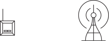
Tandem queues (specifically the minimal 2-nodes case) are then a natural modeling choice for this kind of scenarios, as the first system represents the communication link, while the second one represents the computing-enabled edge node and its task queue. Fig. 1 shows an example: the communication buffer at the sensor and the task queue on the edge computing-enabled Base Station (BS) are the two queues in the tandem.

If the load on the computing-enabled edge node is time constant, while communication is less predictable due to, e.g., dynamic channel variations and random access, then the $M/M/1$ – $M/D/1$ tandem queue is an appropriate model. An $M/M/1$ queue is a proper model for the channel if we assume an ALOHA system [7] with perfect Multi-Packet Reception (MPR), in which [8] the packets are not lost due to collisions and can only be lost due to channel errors. This model is suitable for IoT systems based on Ultra-Narrowband (UNB) transmissions, such as SigFox [9]. On the other hand, computation time is often modeled as a linear function of the data size in the literature [10], and updates of the same size would have a constant and deterministic service time, therefore well-represented by an $M/D/1$ queue. Another option is to consider the computing load as also variable over time, leading to stochastic computing time, and represent the two systems by $M/M/1$ queues with different service rates [11].

An example of the AoI dynamics is plotted in Fig. 2: the AoI grows linearly over time, then decreases instantly when a new update arrives. Naturally, the age at the destination is never lower than the age at the intermediate node, as each packet that reaches the destination has already passed through the intermediate node, but the dynamics between the two are not trivial and serve as a motivation for this work. We analyze the distribution of the PAoI in a tandem queue with two systems with independent service times and a single source, where each infinite queue follows the First Come First Serve (FCFS) policy. We consider both the $M/M/1$ – $M/D/1$ tandem and the $M/M/1$ – $M/M/1$ case, covering common communication relaying and communication and computation scenarios. Our aim is to derive the complete Probability Density Function (PDF) of the PAoI for systems with arbitrary packet generation and service rates, allowing system designers to define reliability requirements using PAoI thresholds and derive the network specifications needed to meet those requirements.

Figure 2: The time-evolution of the Age of Information in a 2-node tandem queue. The age at the destination is plotted in black, the age at the intermediate node is plotted in red. Departures from each node are marked by a circle.

Although the motivation for our analysis is the IoT edge computing, we notice there are other age-sensitive applications that can use the same models and results of this paper. For instance, a tandem queue can model a relay networking in which a packet is transmitted through one or more buffer-aided intermediate nodes between transmitter and receiver to, e.g., overcome the physical distance between the two end-points. A good example is a satellite relay that connects the ground and a satellite (or vice versa) through another satellite. In this case, the links are highly unpredictable and depend on different factors such as positioning jitter [12] and conditions in the upper atmosphere. A tandem queue in which the servers represent the transmission over successive links can represent this kind of system, provided that the service (transmission) times of different links are independent. Blockchain is another application where AoI is a critical metric to validate transactions in real time, particularly when combining the use of the distributed ledger with IoT applications [13]. As nodes need to transmit information, which is then validated, the tandem model is a useful abstraction for the communication and computation time [14].

The contribution of this paper can be summarized by the following points:

• The full PDF of the PAoI is derived for the tandem of an $M/M/1$ and an $M/D/1$ queue, which is relevant for IoT edge computing scenarios;

• The same derivation is performed for the tandem of two $M/M/1$ queues, which can be relevant in relay-based communications with two independent links;

• Design considerations are drawn for the two systems, using the analytical formulas as a basis for system optimization.

The structure of the paper is as follows. In Sec. III the system model is detailed, as well as the procedure to calculate the AoI. Sec. V presents the calculations based on the model for the $M/M/1$ – $M/M/1$ tandem, while Sec. IV does the same for the $M/M/1$ – $M/D/1$ tandem. Numerical results are plotted in Sec. VI, and the paper is concluded in Sec. VII.

II Related work

An overview of edge computing in IoT can be found in [3] and [15]. The initial research approach to latency in the edge paradigm was, in the context of 5G systems, to understand its potential to support Ultra Reliable Low Latency Communication (URLLC) [16, 17, 18]. The relevance of the AoI for edge computing applications was first identified in [5], although only the average AoI is computed. The same authors propose in [19] a joint transmission and computing scheduling for a deadline. Another research area is the use of machine learning, particularly deep learning techniques, to unleash the full potential of IoT edge computing and enable a wider range of application scenarios [20, 21].

AoI is a relatively new metric in networking, but it has gained widespread recognition thanks to its relevance to several applications. Most theoretical results refer to simple queuing systems with a single node and FCFS policy. However, a few recent works focus their attention in the study of the age in tandem queues, even with different policies such as Last Come First Serve (LCFS) [22]. Some IoT scenarios have also been modeled as tandem $M/M/1$, $M/D/1$, or $D/M/1$ queues with multiple sources, as the read from the sensor is first pre-processed, and then transmitted to the server [23]. In this case, each queue follows the FCFS discipline, but the authors derive only the average PAoI. Another possibility is queue replacement, in which only the freshest update for each source is kept in the queue, reducing queue size significantly: in this case, the replaced packet is not placed in the queue, but dropped altogether, reducing channel usage with respect to simple LCFS, with or without preemption. In this case, the queue is modeled as an $M/M/1/2$, and if a new packet arrives it takes the queued packet’s place. Some preliminary results on such a system are given in [24], while the average AoI and PAoI are computed in [25] for one source and in [26] for multiple sources. An analysis of the effect of preemption on this kind of models on the average AoI is presented in [27], and [28] derives the average AoI for two queues in tandem with preemption and different arrival processes. Another work [29] derives the full distribution of the PAoI for preemptive queues whose service time follows a phase-type distribution, which can be used to represent multiple hops. The PDF of the AoI in multi-hop networks with packet preemption has been derived in [30]. Another work [31] deals with multicast networks in which a single source updates multiple receivers over several hops, deriving the average age in that context. Another recent work considers a scenario in which packets that are not received within a deadline are dropped, deriving the average PAoI [32]. Some of these works deal with multi-hop queuing networks, of which our tandem model is a specific case, but they all assume some form of preemption. The computation of AoI and PAoI in systems with preemption is much simpler, particularly in systems of $M/M/1$ queues, but it cannot represent all the relevant use cases: preemption might not be possible or desirable, depending on the specific requirements of the control or monitoring application. For example, telehealth applications might benefit from receiving even out of date samples. To the best of our knowledge, this work is the first to derive the complete PDF of the age for non-preemptive tandem networks, covering these applications. Another example is the satellite relay scenario, where the traffic entering the tandem system comes from an aggregation of devices and therefore each individual update is relevant.

Other works concentrate on more realistic models, considering the effect of physical and medium access issues on the AoI. A model considering a fading wireless channel with retransmissions was used to compute the PAoI distribution over a single-hop link in [33], and a recent live AoI measurement study on a public networks generally confirmed that the theoretical models are realistic [34]. Other works compute the average AoI in Carrier Sense Multiple Access (CSMA) [35], ALOHA [36] and slotted ALOHA [37] networks, considering the impact of the different medium access policies on the age. It is also possible to jointly optimize the sampling and updating processes, i.e., both the reading instants from the sensor and the transmission of updates, if both are controllable [38]: the cost of both operations is a determinant of the overall AoI of the system [39].

A generalization of our model, relevant for applications like satellite relaying, is the multi-hop network with and arbitrary number of $M/M/1$ systems, senders, and receivers: in this case, the moment generating function of the AoI was derived in [40] for preemptive servers. Other scheduling policies make things more complicated: tight bounds for the average AoI were derived in [41] for the FCFS discipline and other AoI-oriented queue prioritization mechanisms.

Deriving the complete distribution of the age might be critical for reliability-oriented applications, but it is still mostly unexplored in the literature: while the work on deriving the first moments of the AoI distribution is extensive, the analytical complexity of deriving the complete PDF is a daunting obstacle. A recent work [42] uses the Chernoff bound to derive an upper bound of the quantile function of the AoI for two queues in tandem with deterministic arrivals, but to the best of our knowledge, the complete PAoI distribution has only been derived for simple queuing systems [33]. Another interesting approach to achieve reliability is to consider the AoI process directly: in [43], the authors use extreme value theory to derive the complementary Cumulative Density Function (CDF) of the PAoI in a realistic channel setting with scheduled transmissions. [44] proposes the use of the risk of ruin, an economic concept, as a metric of fresh and reliable information in augmented reality. Specifically, the CDF of the PAoI is used to find the probability of maximum severity of ruin PAoI in single node systems. Yet another approach to reliability, which does not derive the complete distribution of the AoI but uses an average measure on its tail, is presented in [45]: the authors pose the risk minimization problem as a Markov Decision Process (MDP), optimizing the age with bounded risk. For a more complete overview of the literature on AoI, we refer the reader to [46].

III System model

We consider a tandem system composed by two consecutive queues, where the first one is $M/M/1$. Packets are generated at the first system by a Poisson process with rate $\lambda$ and enter the first queue, whose service time is exponentially distributed with rate $\mu_{1}$. When a packet exits the first system, it enters the second one, whose service time is a constant $D$ or an exponential random variable with rate $\mu_{2}$. A simple diagram of the tandem is shown in Fig. 1. Both queues are of infinite size and are oblivious to the content of the packets: there is no preemption of the updates, i.e. an older packet is not removed from the queue when a new update comes from the same source. As explained in the introduction, we assume that the service times in the two systems are independent. The assumption is realistic for edge computing systems, as the communication and processing are usually independent, but not always verified in relay networks; it therefore needs a careful examination. Even if the service times are independent, however, the waiting times are not, as the queue at the second system depends on the output of the first one. In the following, we use the compact notation $p_{X|Y}(x|y)$ for the conditioned probability $p[X=x|Y=y]$. PDFs are denoted by a lower-case $p$, and CDFs by an upper-case $P$.

In a tandem queue, the packet generation times correspond to the arrival times at the first queue, whereas the receiving instants are the departure times in the second queue. We define the total system time for packet $i$ as $T_{i}$: when a packet is received, the AoI is equal to $T_{i}$, i.e., the difference between the time $r_{i}$ when it is received by the destination and the time $g_{i}$ when it was generated. The PAoI (see Fig. 2) is the maximum value of the AoI, i.e., the age at the instant immediately before the arrival of a new update. If we denote the interarrival time $Y_{i}=g_{i}-g_{i-1}$, then PAoI is given by

$$\Delta_{i}=r_{i}-g_{i-1}=r_{i}-g_{i}+g_{i}-g_{i-1}=T_{i}+Y_{i}$$ (1)

If packet $i$ arrives right after packet $i-1$, it will probably have to wait in the queue for it to depart the system: the system time $T_{i}$ depends on the interarrival time $Y_{i}$. The PDF of the PAoI with value $\tau_{i}$, denoted as $p_{\Delta_{i}}(\tau_{i})$, can then be computed by using the conditional system time probability $p_{T_{i}|Y_{i}}(t_{i}|y_{i})$:

$$p_{\Delta_{i}}(\tau_{i})=\int_{0}^{\tau_{i}}p_{Y_{i}}(y_{i})p_{T_{i}|Y_{i}}(\tau_{i}-y_{i}|y_{i})dy_{i}$$ (2)

We then need to compute $p_{T_{i}|Y_{i}}(t_{i}|y_{i})$. For each system $j=1,2$ in the tandem, the system time $T_{i,j}$ is defined as the sum of the waiting time $W_{i,j}$ and the service time $S_{i,j}$. We also define $Y_{i,j}$, the interarrival time at system $j$. For $j=1$, we have $Y_{i,1}=Y_{i}$, while for $j=2$ :

$$Y_{i,2}=g_{i}+T_{i,1}-(g_{i-1}+T_{i-1,1})=Y_{i}+T_{i,1}-T_{i-1,1}.$$ (3)

Since the first queue is $M/M/1$, the system times for the two queues are independent, as proven by Reich [47] using Burke’s theorem [48] and considering each system in steady state for packet $i-1$. If we consider system $j$ in steady state, i.e., we do not condition on $Y_{i-1,j}$, the system time $T_{i-1,j}$ is exponentially distributed with rate $\alpha_{j}=\mu_{j}-\lambda$. However, the values of $Y_{i}$ and $T_{i}$ are correlated, and the computation of the PAoI needs to account for this fact. In the following, we give the conditional PDF of the components of the PAoI, which will then be joined in the derivation. 6 First, we define the extended waiting time $\Omega_{i,j}$ as the difference between the previous packet’s system time and the interarrival time at the system, i.e., $\Omega_{i,j}=T_{i-1,j}-Y_{i,j}$. The reason we named $\Omega_{i,j}$ the extended waiting time is that $W_{i,j}=[\Omega_{i,j}]^{+}$, where $[x]^{+}$ is equal to $x$ if it is positive and $0$ if $x$ is negative. From the definition of $\Omega_{i,j}$, we have:

$$Y_{i,2} =Y_{i}+(W_{i,1}+S_{i,1})-T_{i-1,1}=S_{i,1}+W_{i,1}-\Omega_{i,1}=S_{i,1}+[-\Omega_{i,1}]^{+}.$$ (4)

since $W_{i,1}-\Omega_{i,1}=[\Omega_{i,1}]^{+}-\Omega_{i,1}=[-\Omega_{i,1}]^{+}$. In the following paragraphs, we derive the PDF of the extended waiting time for the two system types that we are analyzing. Fig. 3 shows a possible realization of a packet’s path through the tandem queue, highlighting the meaning of the extended waiting time: in the first system, in which packet $i$ is queued, it corresponds to the waiting time, while in the second, in which the packet is not queued and enters service immediately, its negative value corresponds to the time between the departure of packet $i-1$ from the second system and the arrival of packet $i$ at the same system. When $W=0$, we have a negative extended waiting time, as packet $i$ arrives after packet $i-1$ leaves the system. In general, we have $\Omega_{i,2}=T_{i-1,2}-Y_{i,2}$, and the system time for packet $i-1$ is $T_{i-1,2}=W_{i-1,2}+D$, while we know the interarrival time $Y_{i,2}=S_{i,1}+[-\Omega_{i,1}]^{+}$.

Figure 3: Schematic of the four steps a packet goes through in a tandem queue, highlighting the components of the PAoI.

Theorem 1.

The CDF of the waiting time for an $M/D/1$ queue with arrival rate $\lambda$ and service time $D$ is:

$$P_{W}(w)=(1-\lambda D)\sum_{k=0}^{\left\lfloor\frac{w}{D}\right\rfloor}\frac{(-\lambda(w-kD))^{k}e^{\lambda(w-kD)}}{k!}.$$ (5)

Proof.

See the derivation by Erlang [49]. ∎

Corollary 1.1.

We can find the queuing time PDF by deriving the CDF from (5):

$$p_{W}(w)=\begin{cases}(1-\lambda D)\left(\lambda e^{\lambda w}+\sum_{k=1}^{\left\lfloor\frac{w}{D}\right\rfloor}\left[\frac{(-\lambda)^{k}(w-kD)^{k-1}e^{\lambda(w-kD)}}{k!}(k+\lambda(w-kD))\right]\right)&w>0;\\ 1-\lambda D&w=0.\end{cases}$$ (6)

The CDF of the waiting time has a discontinuity, as the waiting time is exactly 0 with probability $1-\lambda D$, which corresponds to the probability of the packet finding an empty system and entering service immediately.

Corollary 1.2.

As service time in an $M/D/1$ system is constant, we have the CDF of the total time in the system:

$$P_{T}(t)=P_{W}(t-D)u(t-D).$$ (7)

Corollary 1.3.

The PDF of $\Omega_{i,2}$ conditioned on $S_{i,1}$ and $\Omega_{i,1}$ is given by:

$$p_{\Omega_{i,2}|S_{i,1},\Omega_{i,1}}(\omega_{i,2}|s_{i,1},\omega_{i,1}) =p(W_{i-1,2}+D+S_{i,1}+[-\Omega_{i,1}]^{+}=\omega_{i,2}|S_{i,1}=s_{i,1},\Omega_{i,1}=\omega_{i,1})$$ (8)

$$=p_{W}(\omega_{i,2}+s_{i,1}+[-\omega_{i,1}]^{+}-D).$$

Fig. 4 shows this clearly: when $\Omega_{i,1}$ is negative, the extended queuing time $\Omega_{i,2}$ corresponds to $S_{i,1}+W_{i-1,2}+D-\Omega_{i,1}$, while when $\Omega_{i,1}$ is positive, packet $i$ starts service immediately after packet $i-1$ leaves the first system, and we have $\Omega_{i,2}=S_{i,1}+W_{i-1,2}+D$. The waiting time in $M/D/1$ system is analytically derived, although it can give numeric problems for very large waiting times and high load [50]. If the application requires the computation of very large waiting times with $\lambda D\simeq 1$, we suggest the use of more numerically stable methods from the relevant literature.

Theorem 2.

The PDF of the extended waiting time in a $M/M/1$ - $M/M/1$ tandem queue is given by:

$$p_{\Omega_{i,j}|Y_{i,j}}\left(\omega_{i,j}|y_{i,j}\right) =\alpha_{j}e^{-\alpha_{j}\left(\omega_{i,j}+y_{i,j}\right)}u(\omega_{i,j}+y_{i,j}),$$ (9)

where $u(\cdot)$ is the step function.

Proof.

Knowing the PDF of the system time $T_{i-1,j}$ from well-known results on $M/M/1$ queues, the interarrival time at the first relay $Y_{i,1}$ is exponentially distributed with rate $\lambda$, while in subsequent systems it is given by $Y_{i,2}=S_{i,1}+\left[-\Omega_{i,1}\right]^{+}$. ∎

Corollary 2.1.

We can combine (9) with the definition of $Y_{i,2}$ to get:

$$p_{\Omega_{i,2}|S_{i,1},\Omega_{i,1}}(\omega_{i,2}|s_{i,1},\omega_{i,1})=\alpha_{1}e^{-\alpha_{1}\left(\omega_{i,2}+s_{i,1}+[-\omega_{i,1}]^{+}\right)}u(\omega_{i,2}+s_{i,1}+[-\omega_{i,1}]^{+}).$$ (10)

Figure 4: Schematic of the components of the PAoI. (case $\mathcal{A}$): packet $i$ has to wait in both queues. (case $\mathcal{B}$): packet $i$ waits only in the first queue. (case $\mathcal{C}$): packet $i$ waits only in the second queue. (case $\mathcal{D}$): packet $i$ is immediately served in both systems. Observe the negative expected waiting time $\Omega_{i,j}$ in the cases with empty queue(s).

To compute the exact PDF of PAoI in the 2-system case ($j\in{1,2}$), we distinguish between free and busy systems at each node, i.e., we condition the PDF on the state of each system when packet $i$ arrives to it and calculate it separately for the four possible combinations. Case $\mathcal{A}$ is defined as $\Omega_{i,1}>0\wedge\Omega_{i,2}>0$, while in case $\mathcal{B}$ we have $\Omega_{i,1}>0\wedge\Omega_{i,2}\leq 0$. Similarly, in case $\mathcal{C}$ we have $\Omega_{i,1}\leq 0\wedge\Omega_{i,2}>0$ and in case $\mathcal{D}$ we get $\Omega_{i,1}\leq 0\wedge\Omega_{i,2}\leq 0$. An example of the relevant values in the four cases are shown in Fig. 4: in case $\mathcal{A}$, packet $i$ is queued in both systems, as the previous packet is still in the system when $i$ arrives in each. The two extended queuing times (shown in red) are positive. In case $\mathcal{B}$, packet $i-1$ has already left the second system when packet $i$ leaves the first: the extended queuing time (shown in blue with a dashed outline) is negative, and packet $i$ enters service in the second system as soon as it arrives. In case $\mathcal{C}$, it is the first system that is empty when packet $i$ arrives, and in case $\mathcal{D}$, both systems are empty, and the packet enters service directly at both.

We can then exploit Corollaries 1.1-1.3 to compute the conditioned PDF of the total time at the second system. The PAoI can then simply be computed by unconditioning over the values of $S_{i,1}$, $\Omega_{i,1}$, and $Y_{i}$, simply applying the law of total probability until the PDF for the given case is derived. The division in 4 cases is not strictly necessary, but it reduces the number of terms in the equations considerably with respect to deriving the PDF for the general case directly. The computation for the $M/M/1$ – $M/M/1$ tandem follows the same reasoning, using the results in Theorem 2 and its Corollary 2.1.

Definition 1.

The PDF of the PAoI is:

$$p_{\Delta}(\tau)=p_{\Delta|\mathcal{A}}\left(\tau\right)p(\mathcal{A})+p_{\Delta|\mathcal{B}}\left(\tau\right)p(\mathcal{B})+p_{\Delta|\mathcal{C}}\left(\tau\right)p(\mathcal{C})+p_{\Delta|\mathcal{D}}\left(\tau\right)p(\mathcal{D}).$$ (11)

where $p_{\Delta|\mathcal{X}}$ is the PDF of the PAoI in case $X$ and $p(\mathcal{X})$ is the probability of case $X$ happening. The definition comes from the application of the total law of probability.

In case $\mathcal{A}$, packet $i$ is queued at both systems, and the packet will have the highest queuing delay and system time. The case with the lowest system time is case $\mathcal{D}$, in which the packet experiences no queuing. However, these intuitive relations do not necessarily hold for the PAoI, as the interarrival time between update packets can play a major role. In the analysis of the four cases, we will omit the packet index $i$ wherever possible for the sake of readability. For a quick overview of the notation used in the rest of this paper, we refer the reader to Table I.

TABLE I: Main notation used in the paper.

Symbol	Description
$\lambda$	Packet generation rate
$\mu_{j}$	Service rate of $M/M/1$ system $j$
$D$	Service time of the $M/D/1$ system
$\alpha_{j}=\mu_{j}-\lambda$	Response rate of system $j$
$S_{i,j}$	Service time in system $j$ for packet $i$
$Y_{i,j}$	Interarrival time in system $j$ for packet $i$
$\Omega_{i,j}=T_{i-1,j}-Y_{i,j}$	Extended waiting time in $j$ for packet $i$
$W_{i,j}=[\Omega_{i,j}]^{+}$	Waiting time in system $j$ for packet $i$
$T_{i,j}=S_{i,j}+W_{i,j}$	Total time in system $j$ for packet $i$
$\Delta_{i}=Y_{i}+T_{i}$	PAoI for packet $i$

IV PAoI distribution for the $M/M/1$ – $M/D/1$ tandem

First, we analyze the tandem of an $M/M/1$ and an $M/D/1$ system, using the PDF of the waiting time from (6).

Definition 2.

The auxiliary function $\theta(M,\beta)$, which we will use in the later derivations to make the notation more compact, is defined as:

$$\theta(M,\beta)= \int_{0}^{M}p_{W}(w)e^{\beta w}dw\,\forall\beta\neq 0,\beta\neq-\lambda$$ (12)

$$= \sum_{k=1}^{\left\lfloor\frac{M}{D}\right\rfloor}(1-\lambda D)\int\displaylimits_{kD}^{M}\frac{(-\lambda)^{k}(w-kD))^{k-1}e^{\lambda(w-kD)+\beta w}}{k!}(k+\lambda(w-kD))dw$$

$$+(1-\lambda D)\int\displaylimits_{0}^{M}\lambda e^{(\lambda+\beta)w}dw$$

$$= (1-\lambda D)\Bigg{(}\frac{\lambda(e^{(\lambda+\beta)M}-1)}{\lambda+\beta}+\sum_{k=1}^{\left\lfloor\frac{M}{D}\right\rfloor}\Bigg{[}e^{\beta kD}\bigg{(}\frac{\beta\lambda^{k}}{(\lambda+\beta)^{k+1}}-e^{(\lambda+\beta)(M-kD)}$$

$$\times\bigg{(}\frac{(-\lambda)^{k+1}(M-kD)^{k}}{(\lambda+\beta)k!}+\sum_{j=0}^{k-1}\frac{\lambda^{k}\beta(kD-M)^{j}}{(\lambda+\beta)^{k-j+1}j!}\bigg{)}\bigg{)}\Bigg{]}\Bigg{)}.$$

If $\beta=0$, the result of the integral is simply the waiting time CDF, i.e., $\theta(M,0)=P_{W}(M)$. If $\beta=-\lambda$, we have:

$$\theta(M,-\lambda)= \int_{0}^{M}p_{W}(w)e^{\beta w}dw$$ (13)

$$= (1-\lambda D)\left(\lambda M+\sum_{k=1}^{\left\lfloor\frac{M}{D}\right\rfloor}\int\displaylimits_{kD}^{M}\frac{(-\lambda)^{k}(w-kD))^{k-1}e^{-\lambda kD}}{k!}(k+\lambda(w-kD))dw\right)$$

$$= (1-\lambda D)\left(\lambda M+e^{\beta kD}(-\lambda)^{k}\left(\frac{(M-kD)^{k}}{k!}+\frac{\lambda(M-kD)^{k+1}}{(k+1)!}\right)\right).$$

If we consider a simple $M/D/1$ queue (i.e., not in tandem), it is easy to derive the distribution of the PAoI, as we have

$$\Delta_{i}=D+\max(Y_{i},T_{i-1}).$$ (14)

Therefore, the PAoI is lower than $\tau$ when both $Y_{i}$ and $T_{i-1}$ are smaller than $\tau-D$, and we can write the CDF as:

$$P_{\Delta}(\tau)=\int_{0}^{\tau-D}P_{W}(\tau-2D)\lambda e^{-\lambda y}dy=(1-e^{\lambda(T-\tau)})P_{W}(\tau-2D)u(\tau-2D).$$ (15)

Things are more complex in the tandem system, in which an $M/M/1$ queue feeds the $M/D/1$ queue. Thanks to Burke’s theorem [48], we can consider both systems to be in steady state for packet $i-1$, distinguishing the same four cases $\mathcal{A}$-$\mathcal{D}$ described in Section III and Figure 4.

IV-A The packet is queued at both systems

We start by considering the conditional CDF of the PAoI in case $\mathcal{A}$, in which the $i$-th packet is queued at both systems (i.e., $\Omega_{i,1}>0\wedge\Omega_{i,2}>0$). The probability of a packet being in case $\mathcal{A}$ is given by two concurrent events: first, packet $i$ must find the first system busy, which is equivalent to stating that $T_{i-1,1}>Y_{i}$. Then, the second system must also be busy when the packet arrives to it, so we have $T_{i-1,1}+W_{i-1,2}+S_{i-1,2}>Y_{i}+S_{i,1}$:

$$p(\mathcal{A}) =p(\Omega_{1}>0)p(\Omega_{2}>0|\Omega_{1}>0)$$ (16)

$$=p(Y_{i}<T_{i-1,1},S_{i,1}<T_{i-1,1}-Y_{i}+W_{i-1,2}+D)$$

$$=\int\displaylimits_{0}^{\infty}\int\displaylimits_{0}^{t_{1}}p_{y_{1}}(y_{1})p_{T_{1}}(t_{1})dy_{1}dt_{1}\int\displaylimits_{0}^{\infty}P_{S_{1}}(w+D)p_{W}(w)dw$$

$$=\rho_{1}\left(1-(1-\lambda D)e^{-\mu_{1}D}-e^{-\mu_{1}D}\lim_{M\rightarrow\infty}\theta(M,-\mu_{1})\right)$$

$$=\rho_{1}\left(1-(1-\lambda D)e^{-\mu_{1}D}\left(1+\frac{\lambda(e^{\mu_{1}D}-1)}{\alpha_{1}e^{\mu_{1}D}+\lambda)}\right)\right).$$

The conditioned distribution of the PAoI in case $\mathcal{A}$ is:

$$p_{\Delta_{i}|T_{i-1,1},\mathcal{A}}(\tau|t_{1})= \frac{p_{W}(\tau-t_{1}-2D)P_{Y_{i}+S_{i}}(\tau-D)P_{Y_{i}}(t_{1})}{p(\mathcal{A})}$$ (17)

$$= \frac{p_{W}(\tau-t_{1}-2D)(1-e^{-\lambda t_{1}})(1-e^{-\mu_{1}(\tau-t_{1}-D)})u(\tau-t_{1}-2D)}{p(\mathcal{A})}.$$

We need to consider the case for $w=0$ separately, as there is a discontinuity in the CDF. We can now uncondition the distribution by substituting $p_{W}(w)$ and applying the law of total probability:

$$p_{\Delta|\mathcal{A}}(\tau)= \int\displaylimits_{0}^{\mathclap{\tau-2D}}p_{\Delta_{i}|T_{i-1,1},\mathcal{A}}(\tau|t_{1})\alpha_{1}e^{-\alpha_{1}t_{1}}dt_{1}+\alpha_{1}(1-\lambda D)e^{-\alpha_{1}(\tau-2D)}(1-e^{-\lambda(\tau-2D)}-e^{-\mu_{1}D})$$ (18)

$$= \int\displaylimits_{0}^{\mathclap{\tau-2D}}\frac{\alpha_{1}}{p(\mathcal{A})}\left(e^{\alpha_{1}(w-\tau+2D)}-e^{\mu_{1}(w-\tau+2D)}-e^{-\mu_{1}D-\alpha_{1}(\tau-2D)-\lambda w}+e^{-\mu_{1}(\tau-D)}\right)p_{W}(w)dw$$

$$+\frac{\alpha_{1}(1-\lambda D)}{p(\mathcal{A})}(1-e^{-\lambda t})(1-e^{-\mu_{1}(\tau-t-D)})e^{-\alpha_{1}(\tau-2D)}.$$

We can then substitute the auxiliary function defined in Lemma 2 in (18), getting the PDF of the PAoI in case $\mathcal{A}$:

$$p_{\Delta|\mathcal{A}}(\tau)= \frac{\alpha_{1}}{p(\mathcal{A})}\big{(}e^{-\alpha_{1}(\tau+2D)}\theta(\tau-2D,\alpha_{1})-e^{-\mu_{1}(\tau-2D)}\theta(\tau-2D,\mu_{1})$$ (19)

$$-e^{-\mu_{1}D-\alpha_{1}(\tau-2D)}\theta(\tau-2D,-\lambda)+e^{-\mu_{1}(\tau-D)}(P_{W}(\tau-2D)-(1-\lambda D)\big{)}.$$

IV-B The packet is only queued at the first system

We now consider case $\mathcal{B}$, in which there is queuing at the first system, but not at the second. This is equivalent to stating that $T_{i-1,1}>Y_{i,1}\wedge\Omega_{i-1,2}+D\leq S_{i,1}$. Consequently, we get the following probability for case $\mathcal{B}$:

$$p(\mathcal{B}) =p(\Omega_{1}>0)p(\Omega_{2}\leq 0|\Omega_{1}>0)$$ (20)

$$=p(Y_{i}<T_{i-1,1},S_{i,1}\geq T_{i-1,1}-Y_{i}+W_{i-1,2}+D)$$

$$=\int\displaylimits_{0}^{\infty}\int\displaylimits_{0}^{t_{1}}p_{y_{1}}(y_{1})p_{T_{1}}(t_{1})dy_{1}dt_{1}\int\displaylimits_{0}^{\infty}(1-P_{S_{1}}(w+D))p_{W}(w)dw$$

$$=\rho_{1}e^{-\mu_{1}D}\left((1-\lambda D)+\lim_{M\rightarrow\infty}\theta(M,-\mu_{1})\right)$$

$$=(1-\lambda D)\rho_{1}e^{-\mu_{1}D}\left(1+\frac{\lambda(e^{\mu_{1}D}-1)}{\alpha_{1}e^{\mu_{1}D}+\lambda}\right).$$

The PAoI in this case is given by $T_{i-1,1}+S_{i,1}+D$. Its conditional PDF in this case is given by:

$$p_{\Delta|T_{i-1,1},\mathcal{B}}(\tau|t_{1})= \frac{p_{S_{1}}(\tau-t_{1}-D)P_{Y_{1}}(t_{1})P_{W}(\tau-t_{1}-2D)}{p(\mathcal{B})}$$ (21)

$$= \frac{\mu_{1}e^{-\mu_{1}(\tau-t_{1}-D)}P_{W}(\tau-t_{1}-2D)(1-e^{-\lambda t_{1}})}{p(\mathcal{B})}.$$

We can now uncondition this probability to obtain the PDF of the PAoI in case $\mathcal{B}$:

$$p_{\Delta|\mathcal{B}}(\tau)= \int_{D}^{\tau-D}\frac{P_{W}(s_{1}-D)}{p(\mathcal{B})}\alpha_{1}e^{-\alpha_{1}(\tau-s_{1}-D)}\mu_{1}e^{-\mu_{1}s_{1}}(1-e^{-\lambda(\tau-s_{1}-D)})dx$$ (22)

$$= \alpha_{1}\frac{\mu_{1}}{p(\mathcal{B})}e^{-\alpha_{1}(\tau-D)-\lambda D}\left(\int_{0}^{\tau-2D}P_{W}(w)e^{-\lambda w}dw-\int_{0}^{\tau-2D}P_{W}(w)dw\right)$$

$$= \frac{\alpha_{1}(1-\lambda D)}{\rho_{1}p(\mathcal{B})}e^{-\alpha_{1}(\tau-D)-\lambda D}\sum_{k=0}^{\left\lfloor\frac{\tau-2D}{D}\right\rfloor}\left(e^{-\lambda(\tau-2D)}-\sum_{j=0}^{k+1}\frac{(-\lambda)^{j}(\tau-(k+2)D)^{j}e^{-\lambda kD}}{j!}\right).$$

IV-C The packet is only queued at the second system

We then consider case $\mathcal{C}$, in which there is no queuing at the first system, but the packet is queued at the second. This is equivalent to stating that $T_{i-1,1}\leq Y_{i,1}\wedge\Omega_{i-1,2}+D>S_{i,1}-\Omega_{i,1}$. Consequently, we get the following probability for case $\mathcal{C}$:

$$p(\mathcal{C}) =p(\Omega_{1}\leq 0,\Omega_{2}>0)$$ (23)

$$=p(Y_{i}\geq T_{i-1,1},S_{i,1}<T_{i-1,1}-Y_{i}+W_{i-1,2}+D)$$

$$=\int\displaylimits_{0}^{\infty}\int\displaylimits_{0}^{y_{1}}\int\displaylimits_{\max(0,y_{1}-t_{1}-D)}^{\infty}P_{S_{1}}(w+t_{1}+D-y_{1})p_{W}(w)p_{y_{1}}(y_{1})p_{T_{1}}(t_{1})dwdt_{1}dy_{1}$$

$$=\lambda D-p(\mathcal{A}).$$

The PAoI in this case is given by $T_{i-1,1}+\Omega_{i-1,2}+2D$. Since we know that we are in case $\mathcal{C}$, we have:

$$p_{\Delta|Y_{i,1},\Omega_{i-1,2},\mathcal{C}}(\tau|y_{1},w)= \frac{P_{S_{1}}(\tau-y_{1}-D)P_{Y_{1}}(y_{1})p_{T}(\tau-2D-w)u(y_{1}+w+2D-\tau)}{p(\mathcal{C})}$$ (24)

$$= \frac{\alpha_{1}(1-e^{-\mu_{1}(\tau-y_{1}-D)})e^{\alpha_{1}(w-\tau+2D)}u(y_{1}+w+2D-\tau)}{p(\mathcal{C})}.$$

We can now uncondition this probability on $Y_{i,1}$ by applying the law of total probability:

$$p_{\Delta|\Omega_{i-1,2},\mathcal{C}}(\tau|w)= \int\displaylimits_{\mathclap{\tau-2D-w}}^{\tau-D}\frac{(1-e^{-\mu_{1}(\tau-y_{1}-D)})\lambda e^{-\lambda y_{1}}\alpha_{1}e^{\alpha_{1}(w-\tau+2D)}}{p(\mathcal{C})}dy_{1}$$ (25)

$$= \frac{e^{\mu_{1}(D-\tau)}(\alpha_{1}e^{\mu_{1}(w+D)}-\mu_{1}e^{\alpha_{1}(w+D)}+\lambda)}{p(\mathcal{C})}.$$

We can now uncondition again on $T_{i-1,i}$ and get the PDF of the PAoI in case $\mathcal{D}$:

$$p_{\Delta|\mathcal{C}}(\tau)= \int\displaylimits_{0}^{\tau-2D}p_{\Delta|\Omega_{i-1,2},\mathcal{C}}(\tau|w)p_{W}(w)dw+\frac{1-\lambda D}{p(\mathcal{C})}p_{\Delta|\Omega_{i-1,2},\mathcal{C}}(\tau|0)$$ (26)

$$= \frac{e^{-\mu_{1}(\tau-D)}}{p(\mathcal{C})}\left(\alpha_{1}e^{\mu_{1}D}\theta(\tau-2D,\mu_{1})-\mu_{1}e^{\alpha_{1}D}\theta(\tau-2D,\alpha_{1})+\lambda P_{W}(\tau-2D)\right)$$

$$+\frac{(1-\lambda D)e^{-\mu_{1}(\tau-2D)}}{p(\mathcal{C})}\left(\alpha_{1}-\mu_{1}e^{-\lambda D}+\lambda e^{-\mu_{1}D}\right).$$

IV-D The packet is not queued at either system

Finally, we consider case $\mathcal{D}$, in which there is no queuing at either system. This is equivalent to stating that $T_{i-1,1}\leq Y_{i,1}\wedge\Omega_{i-1,2}+D\leq S_{i,1}-\Omega_{i,1}$. Consequently, we get the following probability for case $\mathcal{D}$:

$$p(\mathcal{D}) =p(\Omega_{1}\leq 0,\Omega_{2}\leq 0)$$ (27)

$$=p(Y_{i}\geq T_{i-1,1},S_{i,1}\geq T_{i-1,1}-Y_{i}+W_{i-1,2}+D)$$

$$=\int\displaylimits_{0}^{\infty}\int\displaylimits_{0}^{y_{1}}\int\displaylimits_{\max(y_{1}-t_{1}-D,0)}^{\infty}(1-P_{S_{1}}(w+t_{1}+D-y_{1}))p_{W}(w)p_{y_{1}}(y_{1})p_{T_{1}}(t_{1})dwdt_{1}dy_{1}$$

$$=(1-\lambda D)-p(\mathcal{B}).$$

The PAoI in this case is given by $Y_{i,1}+S_{i,1}+D$. Since we know that we are in case $\mathcal{D}$, we can apply Bayes’ theorem to get:

$$p_{\Delta|\mathcal{D},Y_{i,1},T_{i-1,1}}(\tau|y_{1},t_{1})= \frac{p_{S_{1}}(\tau-y_{1}-D)P_{Y_{1}}(y_{1})P_{W}(\tau-t_{1}-2D)u(y_{1}-t_{1})}{p(\mathcal{D})}$$ (28)

$$= \frac{\mu_{1}e^{-\mu_{1}(\tau-y_{1}-D)}P_{W}(\tau-t_{1}-2D)u(y_{1}-t_{1})}{p(\mathcal{D})}.$$

We can now uncondition this probability on $Y_{i,1}$ by applying the law of total probability:

$$p_{\Delta|\mathcal{D},T_{i-1,1}}(\tau|t_{1})= \int_{t}^{\tau-D}\frac{\mu_{1}e^{-\mu_{1}(\tau-y_{1}-D)}P_{W}(\tau-t_{1}-2D)u(y_{1}-t_{1})\lambda e^{-\lambda y_{1}}}{p(\mathcal{D})}dy_{1}$$ (29)

$$= \frac{\lambda\mu_{1}}{\alpha_{1}p(\mathcal{D})}P_{W}(\tau-t_{1}-2D)e^{-\mu_{1}(\tau-D)}(e^{\alpha_{1}(\tau-D)}-e^{\alpha_{1}t_{1}}).$$

We can now uncondition again on $T_{i-1,i}$ and get the PDF of the PAoI in case $\mathcal{D}$:

$$p_{\Delta|\mathcal{D}}(\tau)= \int_{D}^{\tau-2D}\frac{\lambda\mu_{1}}{p(\mathcal{D})}P_{W}(\tau-t_{1}-2D)e^{-\mu_{1}(\tau-D)}(e^{\alpha_{1}(\tau-D-t_{1})}-1)dt_{1}$$ (30)

$$= \frac{\lambda\mu_{1}}{p(\mathcal{D})}e^{-\mu_{1}(\tau-D)}\left(e^{\alpha_{1}D}\int_{0}^{\tau-2D}P_{W}(w)e^{\alpha_{1}w}dw-\int_{0}^{\tau-2D}P_{W}(w)dw\right)$$

$$= \frac{\mu_{1}\lambda(1-\lambda D)}{p(\mathcal{D})}e^{-\mu_{1}(\tau-D)}\sum_{k=0}^{\left\lfloor\frac{\tau-2D}{D}\right\rfloor}\Bigg{[}\frac{1}{\lambda}-e^{\alpha_{1}(k+1)D}+\sum_{j=0}^{k}\Bigg{(}\frac{(\tau-(k+2)D)^{j}}{j!}$$

$$\times\left((-\lambda)^{j-1}e^{\lambda(\tau-(k+2)D)}-\frac{\lambda^{k}(-1)^{j}e^{\mu_{1}(\tau-(k+2)D)}}{\mu_{1}^{k-j+1}}\right)\Bigg{)}\Bigg{]}.$$

The overall PAoI PDF is then given by using the previous results for the four cases in Definition 1.

V PAoI distribution for the $M/M/1$ – $M/M/1$ tandem

We now consider the $M/M/1$ – $M/M/1$ tandem, which represents edge computing-enabled systems with stochastic computation times or communication relaying systems. To calculate (11), we divide the computation in 4 cases, as we did in the previous section.

V-A The packet is queued at both systems

We first consider case $\mathcal{A}$, in which packet $i$ finds both systems busy, i.e., the $i$-th packet arrives before the departure of the $(i-1)$-th packet at each system. In this case, $\Omega_{i,1}>0\wedge\Omega_{i,2}>0$. As the conditioned PDF of $\Omega_{i,j}$ was given in (10), and we know that $Y_{i,1}$ is independent from $T_{i-1,1}$, as is $S_{i,1}$ from $T_{i-1,2}$, the probability of this case $p(\mathcal{A})$ is given by:

$$p(\mathcal{A}) =p(\Omega_{1}>0)p(\Omega_{2}>0|\Omega_{1}>0)=$$ (31)

$$=\int\displaylimits_{0}^{\infty}\int\displaylimits_{0}^{t_{1}}p_{y_{1}}(y_{1})p_{T_{1}}(t_{1})dy_{1}dt_{1}\int\displaylimits_{0}^{\infty}\int\displaylimits_{0}^{t_{2}}p_{S_{1}}(s_{1})p_{T_{2}}(t_{2})ds_{1}dt_{2}$$

$$=\frac{\lambda}{\mu_{1}+\alpha_{2}}.$$

We start from the conditioned distribution of the system time on $\Omega_{1}$, $\Omega_{2}$, and $S_{1}$, so $S_{2}$ is the only remaining random variable. In the following, the index $i$ of the packet is omitted where possible to simplify the notation:

$$p_{T|\Omega_{1},\Omega_{2},S_{1},\mathcal{A}}\left(t|\omega_{1},\omega_{2},s_{1}\right)=\mu_{2}e^{-\mu_{2}\left(t-\omega_{1}-s_{1}-\omega_{2}\right)}u(t-\omega_{1}-\omega_{2}-s_{1}).$$ (32)

We now uncondition on $\Omega_{2}$, and then on $S_{1}$, by using the law of total probability:

$$p_{T|\Omega_{1},\mathcal{A}}\left(t|\omega_{1}\right)= \int\displaylimits_{0}^{\mathclap{t-\omega_{1}}}p_{S_{1}}(s_{1})\int\displaylimits_{0}^{\mathclap{t-s_{1}-\omega_{1}}}\frac{p_{\Omega_{2}|\Omega_{1},S_{1}}(\omega_{2}|\omega_{1},s_{1})}{1-P_{\Omega_{2}|\Omega_{1},S_{1}}(0|\omega_{1},s_{1})}p_{T|\Omega_{1},\Omega_{2},S_{1},\mathcal{A}}d\omega_{2}ds_{1}$$ (33)

$$= \frac{\alpha_{2}\mu_{2}(\alpha_{2}+\mu_{1})e^{\shortminus\alpha_{2}(t\shortminus\omega_{1})}(\alpha_{1}+\lambda e^{\shortminus\mu_{1}(t\shortminus\omega_{1})}-\mu_{1}e^{\shortminus\lambda(t\shortminus\omega_{1})})}{\lambda\alpha_{1}\mu_{1}}.$$

The knowledge that we are in case $\mathcal{A}$ means that we have $\Omega_{1}>0$: the denominator in the first integral is the probability of this happening, which we need to account for to get the correct conditional probability. We then condition on $Y_{1}$ and uncondition on $\Omega_{1}$:

$$p_{T|Y_{1},\mathcal{A}}\left(t|y_{1}\right)= \int\displaylimits_{0}^{t}p_{T|\Omega_{1},\mathcal{A}}\left(t|\omega_{1}\right)\frac{p_{\Omega_{1}|Y_{1}}(\omega_{1}|y_{1})}{1-P_{\Omega_{1}|Y_{1}}(0|y_{1})}d\omega_{1}$$ (34)

$$= \frac{\mu_{2}\alpha_{2}e^{-\alpha_{1}y_{1}}}{\lambda p(\mathcal{A})}\Bigg{(}\frac{\alpha_{1}(e^{-\alpha_{1}t}-e^{-\alpha_{2}t})}{(\mu_{2}-\mu_{1})}+\frac{\lambda e^{-\alpha_{1}t}(1-e^{-\mu_{2}t})}{\mu_{2}}-\frac{\mu_{1}(e^{-\alpha_{1}t}-e^{-\mu_{2}t})}{\mu_{2}-\alpha_{1}}\Bigg{)}.$$

We can now derive the PDF of the system time $T$:

$$p_{T|\mathcal{A}}(t)= \int_{0}^{\infty}p_{Y_{1}}(y_{1})p_{T|Y_{1},\mathcal{A}}(t|y_{1})dy_{1}$$ (35)

$$= \frac{\mu_{2}\alpha_{2}}{\mu_{1}p(\mathcal{A})}\Bigg{(}\frac{\alpha_{1}(e^{-\alpha_{1}t}-e^{-\alpha_{2}t})}{(\mu_{2}-\mu_{1})}+\frac{\lambda e^{-\alpha_{1}t}(1-e^{-\mu_{2}t})}{\mu_{2}}-\frac{\mu_{1}(e^{-\alpha_{1}t}-e^{-\mu_{2}t})}{\mu_{2}-\alpha_{1}}\Bigg{)}.$$

Finally, we get the PDF of the PAoI, given by $T+Y_{1}$:

$$p_{\Delta|\mathcal{A}}\left(\tau\right)= \int_{0}^{\tau}p_{T|Y_{1},\mathcal{A}}\left(t|\tau-t\right)p_{Y_{1}}(\tau-t)dt$$ (36)

$$= \frac{\mu_{1}+\alpha_{2}}{\lambda}\bigg{(}\frac{\alpha_{2}\mu_{1}\mu_{2}(e^{-\mu_{1}\tau}-e^{-\mu_{2}\tau})}{(\mu_{2}-\mu_{1})(\mu_{2}-\alpha_{1})}-\lambda e^{-\mu_{1}\tau}(1-e^{-\alpha_{2}\tau})$$

$$+\frac{\alpha_{1}\alpha_{2}\mu_{2}(e^{-\mu_{1}\tau}-e^{-\alpha_{2}\tau})}{(\mu_{2}-\mu_{1})(\mu_{1}-\alpha_{2})}+\frac{\alpha_{1}\mu_{1}\mu_{2}(e^{-\alpha_{1}\tau}-e^{-\mu_{1}\tau})}{(\mu_{2}-\mu_{1})(\mu_{2}-\alpha_{1})}\bigg{)}.$$

V-B The packet is only queued at the first system

We now consider case $\mathcal{B}$, in which the first system is busy but the second one is free when packet $i$ reaches it, i.e., the packet is not queued at the second system. We have $\Omega_{i,1}>0\wedge\Omega_{i,2}\leq 0$, and this case happens with probability $p(\mathcal{B})$:

$$p(\mathcal{B}) =p(\Omega_{1}>0)p(\Omega_{2}\leq 0|\Omega_{1}>0)$$ (37)

$$=\int\displaylimits_{0}^{\infty}\int\displaylimits_{0}^{t_{1}}p_{y_{1}}(y_{1})p_{T_{1}}(t_{1})dy_{1}dt_{1}\int\displaylimits_{0}^{\infty}\int\displaylimits_{t_{2}}^{\infty}p_{S_{1}}(s_{1})p_{T_{2}}(t_{2})ds_{1}dt_{2}$$

$$=\frac{\lambda\alpha_{2}}{\mu_{1}(\mu_{1}+\alpha_{2})}.$$

In this case, the system time PDF is independent of $\Omega_{2}$, and we can just give the conditioned PDF as:

$$p_{T|\Omega_{1},S_{1},\mathcal{B}}\left(t|\omega_{1},s_{1}\right)= \mu_{2}e^{-\mu_{2}(t-\omega_{1}-s_{1})}(1-e^{-\alpha_{2}s_{1}})u(t-\omega_{1}-s_{1}).$$ (38)

As for case $\mathcal{A}$, we condition on $Y_{1}$ and uncondition on $S_{1}$ and $\Omega_{1}$:

$$p_{T|Y_{1},\mathcal{B}}\left(t|y_{1}\right)=\frac{\mu_{1}(\mu_{1}+\alpha_{2})e^{-\alpha_{1}(y_{1}+t)}}{\alpha_{2}}\Bigg{(}1-e^{-\mu_{2}t}-\frac{\alpha_{2}\mu_{2}(1-e^{(\alpha_{1}-\mu_{2})t})}{(\mu_{2}-\mu_{1})(\mu_{2}-\alpha_{1})}+\frac{\alpha_{1}\mu_{2}(1-e^{-\lambda t})}{\lambda(\mu_{2}-\mu_{1})}\Bigg{)}.$$ (39)

From this result, we derive the conditioned PDF of the system time $T$ for case $\mathcal{B}$:

$$p_{T|\mathcal{B}}(t)=\frac{\lambda e^{-\alpha_{1}t}}{p(\mathcal{B})}\Bigg{(}1-e^{-\mu_{2}t}+\frac{\alpha_{1}\mu_{2}(1-e^{-\lambda t})}{\lambda(\mu_{2}-\mu_{1})}-\frac{\alpha_{2}\mu_{2}\left(1-e^{-(\mu_{2}-\alpha_{1})t}\right)}{(\mu_{2}-\mu_{1})(\mu_{2}-\alpha_{1})}\Bigg{)}.$$ (40)

We can now find the unconditioned PDF of the PAoI for case $\mathcal{B}$:

$$p_{\Delta|\mathcal{B}}\left(\tau\right)= \frac{\mu_{1}}{p(\mathcal{B})}(e^{-\alpha_{1}\tau}-e^{-\mu_{1}\tau})-\frac{\lambda\mu_{1}e^{-\mu_{1}\tau}(1-e^{-\alpha_{2}\tau})}{\alpha_{2}p(\mathcal{B})}+\frac{\alpha_{1}\mu_{1}\mu_{2}(e^{-\alpha_{1}\tau}-(1+\lambda\tau)e^{-\mu_{1}\tau})}{\lambda(\mu_{2}-\mu_{1})p(\mathcal{B})}$$ (41)

$$+\frac{\mu_{1}\mu_{2}\alpha_{2}\left((e^{-\mu_{1}\tau}-e^{-\alpha_{1}\tau})(\mu_{2}-\mu_{1})+\lambda(e^{-\mu_{1}\tau}-e^{-\mu_{2}\tau})\right)}{(\mu_{2}-\mu_{1})^{2}(\mu_{2}-\alpha_{1})p(\mathcal{B})}.$$

V-C The packet is only queued at the second system

We can then consider case $\mathcal{C}$, in which the $i$-th packet does not experience any queuing at the first system, i.e., $\Omega_{1}\leq 0$, but there is queuing in the second system, i.e., $\Omega_{2}>0$. The probability of a packet experiencing case $\mathcal{C}$ is given by:

$$p(\mathcal{C}) =p(\Omega_{1}\leq 0,\Omega_{2}>0)$$ (42)

$$=\int\displaylimits_{0}^{\infty}\int\displaylimits_{0}^{y_{1}}\int\displaylimits_{0}^{\infty}p_{y_{1}}(y_{1})p_{T_{1}}(t_{1})p_{S_{1}}(s_{1})\int\displaylimits_{\mathclap{s_{1}-t_{1}+y_{1}}}^{\infty}p_{T_{2}}(t_{2})dt_{2}ds_{1}dt_{1}dy_{1}$$

$$=\frac{\lambda}{\mu_{2}(\mu_{1}+\alpha_{2})}.$$

The conditioned PDF of the system time is:

$$p_{T|\Omega_{1},\Omega_{2},S_{1},\mathcal{C}}\left(t|\omega_{1},\omega_{2},s_{1}\right)=\mu_{2}e^{-\mu_{2}\left(t-s_{1}-\omega_{2}\right)}u(t-s_{1}-\omega_{2}).$$ (43)

As in case $\mathcal{A}$, we condition on $Y_{1}$ and uncondition on $\Omega_{2}$, $S_{1}$, and $\Omega_{1}$:

$$p_{T|Y_{1},\mathcal{C}}\left(t|y_{1}\right)=\frac{\mu_{2}\alpha_{2}e^{-\alpha_{2}t}(e^{-\alpha_{1}y_{1}}-e^{-\alpha_{2}y_{1}})}{\lambda(\mu_{2}-\mu_{1})p(\mathcal{C})}\left(\alpha_{1}-\mu_{1}e^{-\lambda t}+\lambda e^{-\mu_{1}t}\right).$$ (44)

We can now find the PDF of the system delay:

$$p_{T|\mathcal{C}}(t)=\frac{\alpha_{2}e^{-\alpha_{2}t}\left(\alpha_{1}-\mu_{1}e^{-\lambda t}+\lambda e^{-\mu_{1}t}\right)}{\mu_{1}p(\mathcal{C})}.$$ (45)

The conditioned PDF of the PAoI is then:

$$p_{\Delta|\mathcal{C}}(\tau)= \frac{\mu_{2}}{(\mu_{2}-\mu_{1})p(\mathcal{C})}\Bigg{(}\frac{\alpha_{1}\alpha_{2}(e^{-\mu_{1}\tau}-e^{-\alpha_{2}\tau})}{\alpha_{2}-\mu_{1}}+\lambda e^{-\mu_{1}\tau}-\frac{\mu_{1}\alpha_{2}(e^{-\mu_{1}\tau}-e^{-\mu_{2}\tau})}{\mu_{2}-\mu_{1}}$$ (46)

$$-\frac{\alpha_{1}\alpha_{2}(e^{-\alpha_{2}\tau}-e^{-\mu_{2}\tau})}{\lambda}-\lambda e^{-(\mu_{1}+\alpha_{2})\tau}+\alpha_{2}\mu_{1}\tau e^{-\mu_{2}\tau}-\frac{\lambda\alpha_{2}e^{-\mu_{2}\tau}(1-e^{-\alpha_{1}\tau})}{\alpha_{1}}\Bigg{)}.$$

V-D The packet is not queued at either system

Finally, we examine case $\mathcal{D}$, in which the packet experiences no queuing, i.e., $\Omega_{i,1}\leq 0\wedge\Omega_{i,2}\leq 0$. This case happens with probability $p(\mathcal{D})$:

$$p(\mathcal{D})=p(\Omega_{1}\leq 0,\Omega_{2}\leq 0)=\frac{\alpha_{1}\mu_{2}(\mu_{1}+\alpha_{2}))-\lambda\mu_{1}}{\mu_{1}\mu_{2}(\mu_{1}+\alpha_{2})}.$$ (47)

Since the system time probability is independent of $\Omega_{2}$, we can just give the conditioned system time PDF as:

$$p_{T|\Omega_{1},S_{1},\mathcal{D}}\left(t|\omega_{1},s_{1}\right)=\frac{\mu_{1}\mu_{2}e^{-\mu_{2}(t-s_{1})}(1-e^{-\alpha_{2}(s_{1}-\omega_{1})})}{\alpha_{1}}u(t-s_{1}).$$ (48)

We then condition on $Y_{1}$ and uncondition on $S_{1}$ and $\Omega_{1}$:

$$p_{T|Y_{1},\mathcal{D}}\left(t|y_{1}\right)=\frac{\mu_{1}\mu_{2}(e^{-\mu_{1}t}(1-e^{-\alpha_{1}y_{1}})-e^{-\mu_{2}t}(1-e^{-\alpha_{2}y_{1}})+e^{-(\mu_{2}+\alpha_{1})t}(e^{-\alpha_{1}y_{1}}-e^{-\alpha_{2}y_{1}}))}{(\mu_{2}-\mu_{1})p(\mathcal{D})}.$$ (49)

The PDF of the system time is:

$$p_{T|\mathcal{D}}(t)=\frac{\mu_{2}(\mu_{1}-\lambda)e^{-\mu_{1}t}-\mu_{1}(\mu_{2}-\lambda)e^{-\mu_{2}t}}{\lambda(\mu_{2}-\mu_{1})p(\mathcal{D})}+\frac{\lambda e^{-(\mu_{2}+\alpha_{1})t}}{p(\mathcal{D})}.$$ (50)

We can now find the PDF of the PAoI in case $\mathcal{D}$:

$$p_{\Delta|\mathcal{D}}(\tau)=\frac{\mu_{1}\mu_{2}\lambda}{p(\mathcal{D})}\Bigg{(}\frac{\tau(e^{-\mu_{2}\tau}-e^{-\mu_{1}\tau})}{\mu_{2}-\mu_{1}}+\frac{\alpha_{1}e^{-\mu_{2}\tau}-\alpha_{2}e^{-\mu_{1}\tau}}{\alpha_{1}\alpha_{2}(\mu_{2}-\mu_{1})}+\frac{\left(e^{-\lambda\tau}+e^{-(\mu_{1}+\alpha_{2})\tau}\right)}{\alpha_{1}\alpha_{2}}\Bigg{)}.$$ (51)

As for the $M/M/1$ – $M/D/1$ system, the total PDF is given by Theorem 1.

V-E PAoI in the case with equal service rates

In this subsection, we consider a special case in which the general formula of the PAoI PDF is indeterminate, $\mu_{1}=\mu_{2}=\mu$. We follow the same steps as in the normal derivation. The other cases in which the general formula is indeterminate, $\mu_{1}=\alpha_{2}$ and $\mu_{2}=\alpha_{1}$, are not derived in this paper.

In case $\mathcal{A}$, i.e., for $\Omega_{1}>0\wedge\Omega_{2}>0$, we have:

$$p(\mathcal{A})=\frac{\lambda}{\mu+\alpha}.$$ (52)

Following the same steps as in the general case, we get:

$$p_{\Delta|\mathcal{A}}\left(\tau\right)=\frac{e^{-\mu\tau}}{p(\mathcal{A})}\left(\mu(e^{\lambda\tau}-1)+\lambda(e^{-\alpha\tau}-e^{\lambda\tau})+\frac{\mu\alpha(\alpha+\mu)(1-e^{\lambda\tau})+\mu\alpha\lambda\tau(\alpha e^{\lambda\tau}+\mu)}{\lambda^{2}}\right).$$ (53)

The probability of being in case $\mathcal{B}$, i.e., $\Omega_{1}>0\wedge\Omega_{2}\leq 0$, is:

$$p(\mathcal{B})=\frac{\lambda\alpha}{\mu(\mu+\alpha)}.$$ (54)

The conditioned PDF of the PAoI is then:

$$p_{\Delta|\mathcal{B}}\left(\tau\right)=\frac{\mu e^{-\mu\tau}}{p(\mathcal{B})}\Bigg{(}\frac{\alpha^{2}(e^{\lambda\tau}-1)}{\lambda^{2}}-\frac{\lambda(1-e^{-\alpha\tau})}{\alpha}-\frac{\mu(\alpha\lambda\tau^{2}+(\alpha-\lambda)\tau)}{2\lambda}\Bigg{)}.$$ (55)

In this case, as the system is entirely symmetrical and both queues are $M/M/1$, it is also time reversible, making case $\mathcal{B}$ equivalent to case $\mathcal{C}$ in reverse. The probability of being in case $\mathcal{C}$, i.e., $\Omega_{1}\leq 0\wedge\Omega_{2}>0$, and the conditional PDF of the PAoI are then the same as in case $\mathcal{B}$:

$$p(\mathcal{C})= p(\mathcal{B})p_{\Delta|\mathcal{C}}\left(\tau\right)= p_{\Delta|\mathcal{B}}\left(\tau\right).$$ (56)

Finally, we look at case $\mathcal{D}$, in which both systems are free:

$$p(\mathcal{D})=\frac{\alpha(\mu+\alpha)-\lambda}{\mu(\mu+\alpha)}.$$ (57)

We then have the conditioned PDF of the PAoI:

$$p_{\Delta|\mathcal{D}}\left(\tau\right)=\frac{\mu^{2}\lambda e^{-\mu\tau}(2\text{cosh}(\alpha\tau)-\alpha^{2}\tau^{2}-2)}{\alpha^{2}p(\mathcal{D})}.$$ (58)

As in the general case, the overall PAoI is given by Theorem 1.

VI Simulation results

We compared the results of our analysis with a Monte Carlo simulation, transmitting $N=10^{7}$ packets and computing the system delay and PAoI for each. The initial stages of each simulation were discarded, removing $N_{0}=1000$ packets to ensure that the system had reached a steady state. We also divided the packets in the four cases, depending on the queuing they experienced at each system. As the derivation of the PAoI distribution does not involve any approximations, the simulation results should perfectly match the theoretical curves. The Monte Carlo simulation consisted of a single episode, with all packets being transmitted one after the other. The simulation parameters are listed in Table II, and are used for all plots, unless otherwise specified.

TABLE II: Main simulation parameter values (unless otherwise specified).

Parameter	Value	Description
$\lambda$	0.5	Packet generation rate
$\mu_{1}$	1	Service rate of $M/M/1$ system 1
$\mu_{2}$	1.25	Service rate of $M/M/1$ system 2
$D$	0.8	Service time of the $M/D/1$ system
$N$	$10^{7}$	Number of simulated packets
$N_{0}$	1000	Initial transition

VI-A $M/M/1$ – $M/D/1$ tandem

We first consider the tandem in which the first queue is $M/M/1$, while the second is $M/D/1$. We note that, in all the following figures, the simulation results match the theoretically derived curves, showing the soundness of our calculations.

Although not shown, the system time has the expected behavior: it is highest in case $\mathcal{A}$ when the packet is queued at both, and lowest in case $\mathcal{D}$, in which both systems are free. However, the PAoI shows a different trend. While system time increases monotonically with the traffic load, the PAoI is the combination of the system and interarrival time: at one extreme, when the system has very low traffic, it is dominated by the interarrival time, while at the other, it is dominated by the system time. The optimal setting to minimize PAoI is somewhere in the middle, striking a balance between the two causes of age. Furthermore, deterministic service reduces uncertainty, particularly when traffic is high and queuing is the main cause of ageing.

Figure 5: CDF of the PAoI $\Delta$ for the $M/M/1$ – $M/D/1$ tandem in the four subcases.

Fig. 5 shows the CDF of the PAoI in the four cases. It is interesting to note that the PAoI is never smaller than $2D$, as even serving packets instantaneously at the first system would still lead to a minimum delay: once packet $i-1$ is generated, it needs at least a time $D$ to get through the system because of the $M/D/1$ queue, and even if packet $i$ is generated right after it it needs another $D$ to be served by the edge node, leading to a minimum age of $2D$. The PAoI is far smaller in case $\mathcal{C}$, i.e., when the packet is queued only at the $M/D/1$ system, as the queue will often be short and is guaranteed to empty in a limited time. Cases $\mathcal{A}$ and $\mathcal{B}$ show a far worse performance, because of the first system’s lower service rate ($D=0.8$ corresponds to a rate of 1.25) and of its exponential system time distribution. If the packet is not queued at either system (case $\mathcal{D}$), the PAoI is dominated by the interarrival time between the two packets, leading to higher ages.

(a) PAoI for different values of $\lambda$.

(b) PAoI for different values of $\mu_{1}$ and $D$.

Figure 6: CDF of the PAoI $\Delta$ for the $M/M/1$ – $M/M/1$ tandem for different values of $\lambda$, $\mu_{1}$, and $D$.

e can also examine the PAoI as a function of the generation and service rates: Fig. 6(a) shows the PAoI CDF for different values of $\lambda$. We can observe that a value of $\lambda$ close to 0.5 leads to the lowest PAoI, as a high traffic load increases queuing times, while a lower load increases PAoI due to the longer interarrival times. Fig. 6(b) shows what happens when the service rates of the two systems are flipped.

In the figure, we compare two pairs of curves (orange and cyan, violet and black): the orange and violet dashed lines correspond to systems where the second node is faster, the cyan solid line and the black dotted line have the $M/D/1$ queue as the bottleneck. As the system time in the $M/D/1$ queues is rarely very large (it would need a very large queue to be significant, as all packets have the same service time), while $M/M/1$ queues have an exponential system time distribution which can take larger values more often, placing the bottleneck on the $M/D/1$ system leads to a lower PAoI in the worst case (i.e., the larger percentiles), at the cost of a worse PAoI in favorable scenarios. The difference between the orange and black lines is larger than between the cyan and violet ones, as a larger difference between the rates of the two links leads to an increased importance of the bottleneck. As for the subcase analysis, the system time and PAoI from the Monte Carlo simulation follow the analytical curve perfectly. As Fig. 7(b) shows, improving the edge computing capabilities has diminishing returns, as the $M/M/1$ communication system becomes the bottleneck: even with a very low $D$, the PAoI cannot be reduced beyond a certain value without also improving the first system’s capacity.

(a) Percentiles for different values of $\lambda$ with $D=0.8$.

(b) Percentiles for different values of $D$ with optimal $\lambda$.

Figure 7: Tail of the CDF for the $M/M/1$ – $M/D/1$ tandem with $\mu_{1}=1$.

We also make a worst-case analysis as a function of $\lambda$: Fig. 7(a) shows the 95th, 99th and 99.9th percentiles of the PAoI for a system with $\mu_{1}=1$ and $D=0.8$. If the traffic is very high, the queuing time is the dominant factor, causing the worst-case PAoI to diverge. The same happens if the traffic is too low, as the interarrival times can be very large: in this case, the system will almost always be empty, but updates will be very rare. The best performance in terms of PAoI is close to the middle. Depending on the desired reliability, system designers should choose the range of $\lambda$ that fulfils the given percentile of the PAoI in the specific conditions they consider.

VI-B $M/M/1$ – $M/M/1$ tandem

Figure 8: CDF of the PAoI $\Delta$ for the $M/M/1$ – $M/M/1$ tandem in the four subcases.

(a) PAoI for different values of $\lambda$.

(b) PAoI for different values of $\mu_{1}$ and $\mu_{2}$.

Figure 9: CDF of the PAoI $\Delta$ for the $M/M/1$ – $M/M/1$ tandem for different values of $\lambda$, $\mu_{1}$, and $\mu_{2}$.

Fig. 8 shows the PAoI CDF in the four subcases for $\lambda=0.5$, $\mu_{1}=1$, and $\mu_{2}=1.2$. Interestingly, there is no minimum delay and the CDF starts in zero, unlike in the $M/M/1$–$M/D/1$ case. The PAoI is the lowest in case $\mathcal{C}$, and almost identical in cases $B$ and $D$. This is due to the effect of the interarrival times on the PAoI, as case $\mathcal{D}$ usually means that the instantaneous load of the system is low and packets are far apart, increasing the PAoI. In case $\mathcal{C}$, the faster system is busy and the bottleneck is empty. Intuitively, this can reduce age, as the second system will probably be able to serve packets fast enough, but at the same time the instantaneous load will be high enough to avoid having a strong impact on the age.

We can now examine the PAoI CDFs for different values of $\lambda$: the system time is always higher for higher values of $\lambda$, as it depends on the traffic. The same is not true for the PAoI, as Fig. 9(a) shows: as for the $M/M/1$ – $M/D/1$ tandem, the PAoI is lowest for $\lambda=0.5$, as the high interarrival time becomes the dominant factor for $\lambda=0.25$. Interestingly, the gap between the system with $\lambda=0.25$ and the one with $\lambda=0.75$ is wider: the $M/D/1$ system is better able to handle high load situations, as having a high system time is far rarer than in the $M/M/1$. On the other hand, the values of $\mu_{1}$ and $\mu_{2}$ also have an important effect, as Fig. 9(b) shows: while the bottleneck always has a service rate 1, changing the service rate of the other link and even switching the two can have an impact on the PAoI. Naturally, increasing the rate of the other link from 1.2 to 1.6 slightly reduces the PAoI, but we note that for both values, having the first or second system as the bottleneck has a negligible effect on performance. Unlike in the $M/M/1$ – $M/D/1$ tandem, the location of the bottleneck in the tandem seems to have a very small influence on the distribution of the PAoI, as both queues have the same type of service time distribution.

Fig. 10(a) shows how the worst-case PAoI, measured using the 95th, 99th and 99.9th percentiles, changes as a function of $\lambda$. The figure shows that the trends for the two systems are similar: the $M/M/1$ – $M/D/1$ queue can handle a high load slightly better, and its minimum PAoI is lower by 5-10% at all the considered percentiles. In both cases, the optimal $\lambda$ is between 0.45 and 0.5 for all the three percentiles. As for the $M/M/1$ – $M/D/1$ tandem, increasing the rate of the second system gives diminishing returns, and any increase past $\mu_{2}=2$ has negligible benefits if $\mu_{1}=1$, as Fig. 10(b) shows. The horizontal axis in the figure shows the inverse of $\mu_{2}$ to provide a visual comparison with Fig. 7(a): the tail of the PAoI distribution clearly has higher values in the system with two $M/M/1$ queues, as we would expect due to the additional randomness in the service time of the edge computing node.

(a) Percentiles for different values of $\lambda$ with $\mu_{2}=1.25$.

(b) Percentiles for different values of $\mu_{2}$ with optimal $\lambda$.

Figure 10: Tail of the CDF for the $M/M/1$ – $M/M/1$ tandem with $\mu_{1}=1$.

Finally, Fig. 11 shows a comparison of the two kinds of system: as expected, the $M/M/1$ – $M/D/1$ tandem has a higher PAoI in the best-case scenario, as it has a hard minimum of $2D$, but quickly becomes better at the higher percentiles. This difference is more pronounced if the second system is slower, with the $M/M/1$ – $M/D/1$ tandem with $D=1$ having a better PAoI than the $M/M/1$ – $M/M/1$ one with $\mu_{2}=1.25$ for percentiles above the 60th. As the plot shows, the two types of tandem are substantially equivalent if the computation is much faster than the communication. We also show the average PAoI for the two systems in Fig. 12: this is computable from the PDF we derived in this paper, but simpler formulas were derived in the literature [23, 28]. As expected, the $M/M/1$–$M/D/1$ system is better able to deal with high traffic load than the $M/M/1$–$M/M/1$. It is interesting to note that the $M/M/1$–$M/D/1$ queue has a larger gain in the average PAoI than at higher percentiles, even for values of $\lambda$ between 0.45 and 0.5.

Figure 11: CDF of the PAoI $\Delta$ for the two systems (analytical results) for different values of $\mu_{1}$ and $D$.

Figure 12: Average PAoI $\bar{\Delta}$ for the two systems (analytical results) for different values of $\mu_{1}$ and $D$.

VII Conclusions and future work

In this paper, we derived the PDF of the PAoI for a tandem with an $M/M/1$ system followed by an $M/D/1$ and for one consisting of two $M/M/1$ queues. These new results can give more flexibility in the design of bounded AoI systems, both for edge-enabled IoT where the wireless tranmission precedes the computation delay and in other relay applications. The results are derived for two nodes, but the procedure is generic for $K$ $M/M/1$ nodes, potentially followed by an $M/D/1$ system. If the $M/D/1$ system is not the last, the analytical derivation of the PAoI becomes intractable, as its departure process is non-Markovian.

The optimization of the two systems can be a complex operation to perform in real time, and finding the complete PDF analytically might not be manageable in more complex cases with channel errors and multiple sources. However, approximations of the optimal policies can be found by applying deep learning techniques [51], paying particular attention to the uncertainty in the model parameters in order to guarantee reliability even in realistic conditions [52]. The possibility to compute the PDF and CDF using the formulas can provide a fast way to generate samples for a deep learning system, which would then be able to generalize experience in previously unseen situations with a lower computational cost: there is an extensive body of work on similar approaches, which use learning to quickly find a solution to optimization problems with computationally expensive cost functions. Aside from the possibilities offered by deep learning, a possible avenue of future work is the introduction of multiple independent sources in the system, possibly with different priorities. The extension of the system to longer or more complex queuing networks is also a possibility, but the complexity of the derivation might make the analytical results unwieldy. The inclusion of error-prone links, with packets being randomly dropped, is another interesting extension. Finally, the optimization of $\lambda$ in all these scenarios might be a practical application of the theoretical derivations, yielding usable scheduling policies.

References

- [1] M. A. Abd-Elmagid, N. Pappas, and H. S. Dhillon, “On the role of age of information in the Internet of Things,” IEEE Communications Magazine, vol. 57, no. 12, pp. 72–77, Dec. 2019.
- [2] S. Kaul, R. Yates, and M. Gruteser, “Real-time status: How often should one update?” in International Conference on Computer Communications. IEEE, Mar. 2012, pp. 2731–2735.
- [3] W. Yu, F. Liang, X. He, W. G. Hatcher, C. Lu, J. Lin, and X. Yang, “A survey on the edge computing for the Internet of Things,” IEEE access, vol. 6, pp. 6900–6919, Nov. 2017.
- [4] W. Saad, M. Bennis, and M. Chen, “A vision of 6G wireless systems: Applications, trends, technologies, and open research problems,” IEEE network, vol. 34, no. 3, pp. 134–142, Oct. 2019.
- [5] Q. Kuang, J. Gong, X. Chen, and X. Ma, “Age-of-information for computation-intensive messages in mobile edge computing,” in 11th International Conference on Wireless Communications and Signal Processing (WCSP). IEEE, Oct. 2019, pp. 1–6.
- [6] C. Li, S. Li, and Y. T. Hou, “A general model for minimizing age of information at network edge,” in Conference on Computer Communications (INFOCOM). IEEE, Apr. 2019, pp. 118–126.
- [7] N. Abramson, “The ALOHA system: Another alternative for computer communications,” in Fall Joint Computer Conference, ser. AFIPS ’70 (Fall). ACM, Nov. 1970, p. 281–285.
- [8] J. Goseling, Č. Stefanović, and P. Popovski, “A pseudo-Bayesian approach to sign-compute-resolve slotted ALOHA,” in International Conference on Communication Workshop (ICCW). IEEE, Jun. 2015, pp. 2092 – 2096.
- [9] H. Mroue, A. Nasser, S. Hamrioui, B. Parrein, E. Motta-Cruz, and G. Rouyer, “MAC layer-based evaluation of IoT technologies: LoRa, SigFox and NB-IoT,” in Middle East and North Africa Communications Conference (MENACOMM). IEEE, Apr. 2018.
- [10] X. Song, X. Qin, Y. Tao, B. Liu, and P. Zhang, “Age based task scheduling and computation offloading in mobile-edge computing systems,” in Wireless Communications and Networking Conference Workshop (WCNCW). IEEE, Apr. 2019.
- [11] L. Green, “A queueing system in which customers require a random number of servers,” Operations research, vol. 28, no. 6, pp. 1335–1346, Dec. 1980.
- [12] M. Toyoshima, T. Jono, K. Nakagawa, and A. Yamamoto, “Optimum intersatellite link design in the presence of random pointing jitter for free-space laser communication systems,” in Free-Space Laser Communication Technologies XIV, vol. 4635. International Society for Optics and Photonics, Apr. 2002, pp. 95–102.
- [13] S. Lee, M. Kim, J. Lee, R.-H. Hsu, and T. Q. S. Quek, “Is blockchain suitable for data freshness? – age-of-information perspective,” 2020.
- [14] A. Rovira-Sugranes and A. Razi, “Optimizing the Age of Information for blockchain technology with applications to IoT sensors,” IEEE Communications Letters, vol. 24, no. 1, pp. 183–187, Oct. 2019.
- [15] N. Hassan, S. Gillani, E. Ahmed, I. Yaqoob, and M. Imran, “The role of edge computing in internet of things,” IEEE Communications Magazine, vol. 56, no. 11, pp. 110–115, 2018.
- [16] M. S. Elbamby, M. Bennis, W. Saad, and et al., “Proactive edge computing in fog networks with latency and reliability guarantees,” EURASIP Journal on Wireless Communications and Networking, vol. 209, no. 1, 2018.
- [17] M. S. Elbamby, C. Perfecto, C. Liu, J. Park, S. Samarakoon, X. Chen, and M. Bennis, “Wireless edge computing with latency and reliability guarantees,” Proceedings of the IEEE, vol. 107, no. 8, pp. 1717–1737, 2019.
- [18] Y. Hu and A. Schmeink, “Delay-constrained communication in edge computing networks,” in 2018 IEEE 19th International Workshop on Signal Processing Advances in Wireless Communications (SPAWC), 2018, pp. 1–5.
- [19] J. Gong, G. Kuang, and X. Chen, “Joint transmission and computing scheduling forstatus update with mobile edge computing,” arXiv preprint arXiv:2002.09719, Feb. 2020.
- [20] X. Wang, Y. Han, V. C. M. Leung, D. Niyato, X. Yan, and X. Chen, “Convergence of edge computing and deep learning: A comprehensive survey,” IEEE Communications Surveys Tutorials, vol. 22, no. 2, pp. 869–904, 2020.
- [21] H. Li, K. Ota, and M. Dong, “Learning IoT in edge: Deep learning for the Internet of Things with edge computing,” IEEE Network, vol. 32, no. 1, pp. 96–101, Jan. 2018.
- [22] A. M. Bedewy, Y. Sun, and N. B. Shroff, “Age-optimal information updates in multihop networks,” in International Symposium on Information Theory (ISIT). IEEE, Jun. 2017, pp. 576–580.
- [23] C. Xu, H. H. Yang, X. Wang, and T. Q. Quek, “Optimizing information freshness in computing enabled IoT networks,” IEEE Internet of Things Journal, Oct. 2019.
- [24] N. Pappas, J. Gunnarsson, L. Kratz, M. Kountouris, and V. Angelakis, “Age of information of multiple sources with queue management,” in International Conference on Communications (ICC). IEEE, Jun. 2015, pp. 5935–5940.
- [25] A. Kosta, N. Pappas, A. Ephremides, and V. Angelakis, “Queue management for age sensitive status updates,” in International Symposium on Information Theory (ISIT). IEEE, Jul. 2019, pp. 330–334.
- [26] ——, “Age of information performance of multiaccess strategies with packet management,” Journal of Communications and Networks, vol. 21, no. 3, pp. 244–255, Jun. 2019.
- [27] R. D. Yates, “Age of information in a network of preemptive servers,” in Conference on Computer Communications Workshops (INFOCOM WKSHPS). IEEE, Apr. 2018, pp. 118–123.
- [28] C. Kam, J. P. Molnar, and S. Kompella, “Age of information for queues in tandem,” in Military Communications Conference (MILCOM). IEEE, Oct. 2018, pp. 1–6.
- [29] N. Akar, O. Doğan, and E. U. Atay, “Finding the exact distribution of (Peak) Age of Information for queues of PH/PH/1/1 and M/PH/1/2 type,” IEEE Transactions on Communications, vol. 68, no. 9, pp. 5661–5672, Jun. 2020.
- [30] O. Ayan, H. Murat Gürsu, A. Papa, and W. Kellerer, “Probability analysis of age of information in multi-hop networks,” IEEE Networking Letters, vol. 2, no. 2, pp. 76–80, 2020.
- [31] B. Buyukates, A. Soysal, and S. Ulukus, “Age of information in multihop multicast networks,” Journal of Communications and Networks, vol. 21, no. 3, pp. 256–267, Jul. 2019.
- [32] J. Li, Y. Zhou, and H. Chen, “Age of information for multicast transmission with fixed and random deadlines in IoT systems,” IEEE Internet of Things Journal, Mar. 2020.
- [33] R. Devassy, G. Durisi, G. C. Ferrante, O. Simeone, and E. Uysal, “Reliable transmission of short packets through queues and noisy channels under latency and peak-age violation guarantees,” IEEE Journal on Selected Areas in Communications, vol. 37, no. 4, pp. 721–734, Feb. 2019.
- [34] H. B. Beytur, S. Baghaee, and E. Uysal, “Measuring age of information on real-life connections,” in 27th Signal Processing and Communications Applications Conference (SIU). IEEE, Apr. 2019, pp. 1–4.
- [35] A. Maatouk, M. Assaad, and A. Ephremides, “On the age of information in a csma environment,” IEEE/ACM Transactions on Networking, vol. 28, no. 2, pp. 818–831, Feb. 2020.
- [36] R. D. Yates and S. K. Kaul, “Age of Information in uncoordinated unslotted updating,” arXiv preprint arXiv:2002.02026, Feb. 2020.
- [37] X. Chen, K. Gatsis, H. Hassani, and S. S. Bidokhti, “Age of information in random access channels,” in International Symposium on Information Theory (ISIT). IEEE, Jun. 2020, pp. 1770–1775.
- [38] R. Li, Q. Ma, J. Gong, Z. Zhou, and X. Chen, “Age of processing: Age-driven status sampling and processing offloading for edge computing-enabled real-time IoT applications,” arXiv preprint arXiv:2003.10916, Mar. 2020.
- [39] B. Zhou and W. Saad, “Joint status sampling and updating for minimizing age of information in the Internet of Things,” IEEE Transactions on Communications, vol. 67, no. 11, pp. 7468–7482, Jul. 2019.
- [40] R. D. Yates, “The age of information in networks: Moments, distributions, and sampling,” IEEE Transactions on Information Theory, Sep. 2020.
- [41] F. Chiariotti, O. Vikhrova, B. Soret, and P. Popovski, “Information freshness of updates sent over LEO satellite multi-hop networks,” arXiv preprint arXiv:2007.05449, Jul. 2020.
- [42] J. P. Champati, H. Al-Zubaidy, and J. Gross, “Statistical guarantee optimization for AoI in single-hop and two-hop systems with periodic arrivals,” arXiv preprint arXiv:1910.09949, Oct. 2019.
- [43] C.-F. Liu and M. Bennis, “Taming the tail of maximal information age in wireless industrial networks,” IEEE Communications Letters, vol. 23, no. 12, pp. 2442–2446, Sep. 2019.
- [44] C. Chaccour and W. Saad, “On the ruin of age of information in augmented reality over wireless teraherts (thz) networks,” in Globecom. IEEE, Dec. 2020.
- [45] B. Zhou, W. Saad, M. Bennis, and P. Popovski, “Risk-aware optimization of Age of Information in the Internet of Things,” arXiv preprint arXiv:2002.09805, Feb. 2020.
- [46] R. D. Yates, Y. Sun, D. R. Brown III, S. K. Kaul, E. Modiano, and S. Ulukus, “Age of information: An introduction and survey,” arXiv preprint arXiv:2007.08564, Jul. 2020.
- [47] E. Reich, “Note on queues in tandem,” The Annals of Mathematical Statistics, vol. 34, no. 1, pp. 338–341, Mar. 1963.
- [48] P. J. Burke, “The output of a queuing system,” Operations Research, vol. 4, no. 6, pp. 699–704, Dec. 1956.
- [49] A. Erlang, “Telefon-ventetider. et stykke sandsynlighedsregning,” Matematisk tidsskrift. B, pp. 25–42, Jan. 1920.
- [50] V. B. Iversen and L. Staalhagen, “Waiting time distribution in M/D/1 queueing systems,” Electronics Letters, vol. 35, no. 25, pp. 2184–2185, Dec. 1999.
- [51] C. She, C. Sun, Z. Gu, Y. Li, C. Yang, H. V. Poor, and B. Vucetic, “A tutorial of ultra-reliable and low-latency communications in 6G: Integrating theoretical knowledge into deep learning,” arXiv preprint arXiv:2009.06010, Sep. 2020.
- [52] M. Angjelichinoski, K. F. Trillingsgaard, and P. Popovski, “A statistical learning approach to ultra-reliable low latency communication,” IEEE Transactions on Communications, vol. 67, no. 7, pp. 5153–5166, Mar. 2019.