Neutron dominance in excited states of ²⁶Mg and ¹⁰Be probed by proton and alpha inelastic scattering

Abstract

Isospin characters of nuclear excitations in ²⁶Mg and ¹⁰Be are investigated via proton ($p$) and alpha ($\alpha$) inelastic scattering. A structure model of antisymmetrized molecular dynamics (AMD) is applied to calculate the ground and excited states of ²⁶Mg and ¹⁰Be. The calculation describes the isoscalar feature of the ground-band $2^{+}_{1}$($K^{\pi}=0^{+}_{1}$) excitation and predicts the neutron dominance of the side-band $2^{+}_{2}$($K^{\pi}=2^{+}$) excitation in ²⁶Mg and ¹⁰Be. The $p$ and $\alpha$ inelastic scattering off ²⁶Mg and ¹⁰Be is calculated by microscopic coupled-channel (MCC) calculations with a $g$-matrix folding approach by using the matter and transition densities of the target nuclei calculated with AMD. The calculation reasonably reproduces the observed $0^{+}_{1}$, $2^{+}_{1}$, and $2^{+}_{2}$ cross sections of ²⁶Mg+$p$ scattering at incident energies $E_{p}=24$ and 40 MeV and of ²⁶Mg+$\alpha$ scattering at $E_{\alpha}=104$ and 120 MeV. For ¹⁰Be+$p$ and ¹⁰Be+$\alpha$ scattering, inelastic cross sections to the excited states in the $K^{\pi}=0^{+}_{1}$ ground-, $K^{\pi}=2^{+}$ side-, $K^{\pi}=0^{+}_{2}$ cluster-, and $K^{\pi}=1^{-}$ cluster-bands are investigated. The isospin characters of excitations are investigated via inelastic scattering processes by comparison of the production rates in the ¹⁰Be+$p$, ¹⁰Be+$\alpha$, and ¹⁰C+$p$ reactions. The result predicts that the $2^{+}_{2}$ state is selectively produced by the ¹⁰Be+$p$ reaction because of the neutron dominance in the $2^{+}_{2}$ excitation as in the case of the ²⁶Mg+$p$ scattering to the $2^{+}_{2}$ state, whereas its production is significantly suppressed in the ¹⁰C+$p$ reaction.

I Introduction

Isospin characters of nuclear excitations in $Z\neq N$ nuclei have been attracting great interests. To discuss the difference between neutron and proton components in nuclear deformations and excitations, the neutron and proton transition matrix elements, $M_{n}$ and $M_{p}$, have been extensively investigated by experimental works with mirror analysis of electric transitions and hadron inelastic scattering with $\alpha$, $p$, and $\pi^{-}/\pi^{+}$ as well as electron inelastic scattering. The ratio $M_{n}/M_{p}$ has been discussed with the isoscalar and isovector components of $2^{+}$ excitations for various stable nuclei Bernstein:1977wtr ; Bernstein:1979zza ; Bernstein:1981fp ; Brown:1980zzd ; Brown:1982zz . The simple relation $M_{n}/M_{p}=N/Z$ is naively expected for a uniform rigid rotor model, while $M_{n}/M_{p}=1$ should be satisfied if only a $Z=N$ core part contributes to the excitation. In the analysis of the $M_{n}/M_{p}$ ratio, it has been reported that $M_{n}/M_{p}$ systematically exceeds $N/Z$ in proton closed-shell nuclei. In particular, an extremely large value of the ratio was found in ¹⁸O, which expresses remarkable neutron dominance of the $2^{+}_{1}$ excitation. In the opposite case, $M_{n}/M_{p}<N/Z$ of proton dominance was obtained in neutron closed-shell nuclei.

For ²⁶Mg, the $M_{n}/M_{p}$ ratio has been investigated for various excited states by means of life-time measurements of mirror transitions Alexander:1982sph , and $\pi^{-}/\pi^{+}$, $p$, and $\alpha$ Wiedner:1980cea ; Alons:1981rrm ; Zwieglinski:1983zz ; VanDerBorg:1981qiu inelastic scattering. In those analyses, the strong state dependency of isospin characters has been found in the first and second $2^{+}$ states. The ratio $M_{n}/M_{p}=0.7$–1 was obtained for the $0^{+}_{1}\to 2^{+}_{1}$ transition, whereas $M_{n}/M_{p}=1.2$–4 was estimated for the $0^{+}_{1}\to 2^{+}_{2}$ transition. The former indicates an approximately isoscalar nature of the $2^{+}_{1}$ excitation, while the latter shows predominant neutron component of the $2^{+}_{2}$ excitation. However, there remains significant uncertainty in the neutron component of the $0^{+}_{1}\to 2^{+}_{2}$ transition.

The isospin characters of nuclear excitations are hot issues also in the physics of unstable nuclei. The neutron dominance in the $2^{+}_{1}$ state has been suggested in neutron-rich nuclei such as ¹²Be and ¹⁶C Kanada-Enyo:1996zsp ; Iwasaki:2000gh ; Kanada-Enyo:2004tao ; Kanada-Enyo:2004ere ; Sagawa:2004ut ; Takashina:2005bs ; Ong:2006rm ; Burvenich:2008zz ; Takashina:2008zza ; Elekes:2008zz ; Wiedeking:2008zzb ; Yao:2011zza ; Forssen:2011dr . The proton component can be determined from $B(E2)$ measured by $\gamma$ decays. For the neutron component, such tools as mirror analysis and $\pi^{-}/\pi^{+}$ scattering are practically difficult for neutron-rich nuclei. Instead, $p$ inelastic scattering experiments in the inverse kinematics have been intensively performed to probe the neutron component and supported the neutron dominance in the $2^{+}_{1}$ state of ¹²Be and ¹⁶C. Very recently, Furuno et al. have achieved an $\alpha$ inelastic scattering experiment off ${}^{10}\textrm{C}$ in the inverse kinematics and discussed the isospin characters of the $2^{+}_{1}$ excitation Furuno:2019lyp .

Our aim in this paper is to investigate isospin characters of the $2^{+}_{1}$ and $2^{+}_{2}$ excitations in ${}^{26}\textrm{Mg}$ and ${}^{10}\textrm{Be}$ with microscopic coupled-channel (MCC) calculations of $p$ and $\alpha$ scattering. We also aim to predict inelastic cross sections to cluster excitations of ${}^{10}\textrm{Be}$. Structures of the ground and excited states of ${}^{10}\textrm{Be}$ have been studied with many theoretical models, and described well by the cluster structure of $2\alpha+nn$ (see Refs. Oertzen-rev ; KanadaEn'yo:2012bj ; Ito2014-rev and references therein). In Ref. Kanada-Enyo:2011plo , one of the authors (Y. K-E.) has discussed the $2^{+}_{1}$ and $2^{+}_{2}$ excitations of ${}^{10}\textrm{Be}$ with the isovector triaxiality, and predicted the neutron dominance in the $2^{+}_{2}$ excitation similarly to that of ${}^{26}\textrm{Mg}$.

In the present MCC calculations, the nucleon-nucleus potentials are microscopically derived by folding the Melbourne $g$-matrix $NN$ interaction with diagonal and transition densities of target nuclei, which are obtained from microscopic structure models. The $\alpha$-nucleus potentials are obtained by folding the nucleon-nucleus potentials with an $\alpha$ density. The MCC approach with the Melbourne $g$-matrix $NN$ interaction has successfully described the observed cross sections of $p$ and $\alpha$ elastic and inelastic scattering off various nuclei at $p$ energies from 40 MeV to 300 MeV and $\alpha$ energies from 100 MeV to 400 MeV Amos:2000 ; Karataglidis:2007yj ; Minomo:2009ds ; Toyokawa:2013uua ; Minomo:2017hjl ; Egashira:2014zda ; Minomo:2016hgc . In our recent works Kanada-Enyo:2019prr ; Kanada-Enyo:2019qbp ; Kanada-Enyo:2019uvg ; Kanada-Enyo:2020zpl , we have applied the MCC calculations by using matter and transition densities of target nuclei calculated by a structure model of antisymmetrized molecular dynamics (AMD) KanadaEnyo:1995tb ; KanadaEn'yo:1998rf ; Kanada-Enyo:1999bsw ; KanadaEn'yo:2012bj and investigated transition properties of low-lying states of various stable and unstable nuclei via $p$ and $\alpha$ inelastic scattering. One of the advantages of this approach is that one can discuss inelastic processes of different hadronic probes, $p$ and $\alpha$, in a unified treatment of a microscopic description. Another advantage is that there is no phenomenological parameter in the reaction part. Since one can obtain cross sections at given energies for given structure inputs with no ambiguity, it can test the validity of the structure inputs via $p$ and $\alpha$ cross sections straightforwardly.

In this paper, we apply the MCC approach to $p$ and $\alpha$ scattering off ${}^{26}\textrm{Mg}$ and ${}^{10}\textrm{Be}$ using the AMD densities of the target nuclei, and investigate isospin characters of inelastic transitions of ${}^{26}\textrm{Mg}$ and ${}^{10}\textrm{Be}$. Particular attention is paid on transition features of the ground-band $2^{+}_{1}$ state and the side-band $2^{+}_{2}$ state. We also give theoretical a prediction of inelastic cross sections to cluster states of $A=10$ nuclei of the ${}^{10}\textrm{Be}+p$, ${}^{10}\textrm{Be}+\alpha$, and ${}^{10}\textrm{C}+p$ reactions.

The paper is organized as follows. The next section briefly describes the MCC approach for the reaction calculations of $p$ and $\alpha$ scattering and the AMD framework for structure calculations of ${}^{26}\textrm{Mg}$ and ${}^{10}\textrm{Be}$. Structure properties of ${}^{26}\textrm{Mg}$ and ${}^{10}\textrm{Be}$ are described in Sec. III, and transition properties and $p$ and $\alpha$ scattering are discussed in Sec. IV. Finally, the paper is summarized in Sec. V.

II Method

The reaction calculations of $p$ and $\alpha$ scattering are performed with the MCC approach as done in Refs. Kanada-Enyo:2019prr ; Kanada-Enyo:2019qbp ; Kanada-Enyo:2019uvg . The diagonal and coupling potentials for the nucleon-nucleus system are microscopically calculated by folding the Melbourne $g$-matrix $NN$ interaction Amos:2000 with densities of the target nucleus calculated by AMD. The $\alpha$-nucleus potentials are obtained in an extended nucleon-nucleus folding model Egashira:2014zda by folding the nucleon-nucleus potentials with an $\alpha$ density given by a one-range Gaussian form. In the present reaction calculations, the spin-orbit term of the potentials is not taken into account to avoid complexity as in Refs. Kanada-Enyo:2019uvg ; Kanada-Enyo:2020zpl . It should be stressed again that there is no adjustable parameter in the reaction part. Therefore, nucleon-nucleus and $\alpha$-nucleus potentials are straightforwardly obtained from given structure inputs of diagonal and transition densities. The adopted channels of the MCC calculations are explained in Sec. IV.

The structure calculation of ${}^{10}\textrm{Be}$ has been done by AMD with variation after parity and total angular momentum projections (VAP) in Ref. Kanada-Enyo:1999bsw . The diagonal and transition densities obtained by AMD have been used for the MCC calculation of the ${}^{10}\textrm{Be}+p$ reaction in the previous work Kanada-Enyo:2019uvg . We adopt the AMD results of ${}^{10}\textrm{Be}$ as structure inputs of the present MCC calculations of the ${}^{10}\textrm{Be}+p$ and ${}^{10}\textrm{Be}+\alpha$ reactions. For ${}^{26}\textrm{Mg}$, we apply the AMD+VAP with fixed nucleon spins in the same way Ref. Kanada-Enyo:2020zpl for ²⁸Si. Below, we briefly explain the AMD framework of the present calculation of ${}^{26}\textrm{Mg}$. This calculation is an extension of the previous AMD calculation of ${}^{26}\textrm{Mg}$ in Ref. Kanada-Enyo:2011plo . For more details, the reader is referred to the previous works and references therein.

An AMD wave function of a mass-number $A$ nucleus is given by a Slater determinant of single-nucleon Gaussian wave functions as

$$\Phi_{\rm AMD}({\boldsymbol{Z}}) = \frac{1}{\sqrt{A!}}{\cal{A}}\{\varphi_{1},\varphi_{2},\ldots,\varphi_{A}\},$$ (1)

$$\varphi_{i} = \phi_{{\boldsymbol{X}}_{i}}\chi_{i}\tau_{i},$$ (2)

$$\phi_{{\boldsymbol{X}}_{i}}({\boldsymbol{r}}_{j}) = \left(\frac{2\nu}{\pi}\right)^{3/4}\exp\bigl{[}-\nu({\boldsymbol{r}}_{j}-\boldsymbol{X}_{i})^{2}\bigr{]}.$$ (3)

Here ${\cal{A}}$ is the antisymmetrizer, and $\varphi_{i}$ is the $i$th single-particle wave function given by a product of spatial ($\phi_{{\boldsymbol{X}}_{i}}$), nucleon-spin ($\chi_{i}$), and isospin ($\tau_{i}$) wave functions. In the present calculation of ${}^{26}\textrm{Mg}$, we fix nucleon spin and isospin functions as spin-up and spin-down states of protons and neutrons. Gaussian centroid parameters $\{\boldsymbol{X}_{i}\}$ for single-particle wave functions are treated as complex variational parameters independently for all nucleons.

In the model space of the AMD wave function, we perform energy variation after total-angular-momentum and parity projections (VAP). For each $J^{\pi}$ state, the variation is performed with respect to the $J^{\pi}$-projected wave function $P^{J\pi}_{MK}\Phi_{\rm AMD}({\boldsymbol{Z}})$ to obtain the optimum parameter set of Gaussian centroids $\{\boldsymbol{X}_{i}\}$. Here $P^{J\pi}_{MK}$ is the total angular momentum and parity projection operator. In the energy variation, $K=0$ is taken for the $J^{\pi}=0^{+}$, $2^{+}$, and $4^{+}$ states in the $K^{\pi}=0^{+}_{1}$ ground-band, and $K=2$ is chosen for the $J^{\pi}=2^{+}$ and $3^{+}$ states in the $K^{\pi}=2^{+}$ side-band. After the energy variation of these states, we obtain five basis wave functions. To obtain final wave functions of ${}^{26}\textrm{Mg}$, mixing of the five configurations (configuration mixing) and $K$-mixing are taken into account by diagonalizing the norm and Hamiltonian matrices.

In the present calculation of ${}^{26}\textrm{Mg}$, the width parameter $\nu=0.15$ fm^-2 is used. The effective nuclear interactions of structure calculation for ${}^{26}\textrm{Mg}$ are the MV1 (case 1) central force TOHSAKI supplemented by a spin-orbit term of the G3RS force LS1 ; LS2 . The Bartlett, Heisenberg, and Majorana parameters of the MV1 force are $b=h=0$ and $m=0.62$, and the spin-orbit strengths are $u_{I}=-u_{II}=2800$ MeV. The Coulomb force is also included. All these parameters of the Gaussian width and effective interactions are the same as those used in the previous studies of ${}^{26}\textrm{Mg}$, ²⁶Si, and ²⁸Si of Refs. Kanada-Enyo:2004ere ; Kanada-Enyo:2011plo . A difference is the variational procedure. The variation was done before the total angular momentum projection in the previous studies, but it is done after the total angular momentum projection in the present AMD+VAP calculation.

III Energy levels, radii, and $B(E2)$ of target nuclei

III.1 Structure of ${}^{26}\textrm{Mg}$

The ground and excited states of ${}^{26}\textrm{Mg}$ obtained after the diagonalization contain some amount of the configuration- and $K$-mixing, but they are approximately classified into the $K^{\pi}=0^{+}_{1}$ band built on the $0^{+}_{1}$ state and those in the $K^{\pi}=2^{+}$ band starting from the $2^{+}_{2}$ state. In Fig. 1(a), the calculated energy spectra are shown in comparison with the experimental spectra of candidate states for the $K^{\pi}=0^{+}_{1}$ and $K^{\pi}=2^{+}$ band members. The experimental $0^{+}_{1}$, $2^{+}_{1}(1.81)$, and $4^{+}_{2}(4.90)$ states are considered to belong the $K^{\pi}=0^{+}_{1}$ band, and the $2^{+}_{2}(2.94)$, $3^{+}_{2}(4.35)$, and $4^{+}_{4}(5.72)$ states are tentatively assigned to the $K^{\pi}=2^{+}$ band from $\gamma$-decay properties Nagel:1974 . However, there are other candidates such as the $3^{+}_{1}(3.94)$, $4^{+}_{1}(4.32)$, and $4^{+}_{3}(5.48)$ states in the same energy region. We denote the theoretical states in the $K^{\pi}=0^{+}_{1}$ band as $J^{\pi}=\{0^{+}_{1}$, $2^{+}_{1}$, and $4^{+}_{\textrm{gs}}\}$ and those in the $K^{\pi}=2^{+}$ band as $J^{\pi}=\{2^{+}_{2}$, $3^{+}_{K2}$, and $4^{+}_{K2}\}$, and tentatively assign the $K^{\pi}=0^{+}_{1}$ band members to {$0^{+}_{1}$, $2^{+}_{1}(1.81)$, $4^{+}_{2}(4.90)$} and the $K^{\pi}=2^{+}$ band members to {$2^{+}_{2}(2.94)$, $3^{+}_{2}(4.35)$, $4^{+}_{4}(5.72)$}, though uncertainty remains in assignments of $3^{+}$ and $4^{+}$ states.

The root-mean-square (rms) radii of proton $(R_{p}$), neutron $(R_{n}$), and matter $(R_{m}$) distributions of the band-head states of ${}^{26}\textrm{Mg}$ are shown in Table 1. The $E\lambda$ transition strength $B(E\lambda)$ of the transition $J^{\pi}_{i}\to J^{\pi}_{f}$ is given by the proton component of the matrix element $M_{p}$ as

$$B(E\lambda;J^{\pi}_{i}\to J^{\pi}_{f})\equiv\frac{1}{2J_{i}+1}|M_{p}|^{2},$$ (4)

and its counter part (the neutron component $B_{n}(E\lambda)$) is given by $M_{n}$ as

$$B_{n}(E\lambda;J^{\pi}_{i}\to J^{\pi}_{f})\equiv\frac{1}{2J_{i}+1}|M_{n}|^{2}.$$ (5)

In Table 2, the theoretical values of $B(E2)$ and $B_{n}(E2)$ obtained by AMD, and the observed $E2$ transition strengths are listed.

In each group of {$0^{+}_{1}$, $2^{+}_{1}(1.81)$, $4^{+}_{2}(4.90)$} and {$2^{+}_{2}(2.94)$, $3^{+}_{2}(4.35)$, $4^{+}_{4}(5.72)$}, sequences of strong $\gamma$ transitions have been observed and support the assignment of the $K^{\pi}=0^{+}_{1}$ and $K^{\pi}=2^{+}$ bands. However, possible state mixing between the $4^{+}_{1}(4.32)$ and $4^{+}_{2}(4.90)$ states in the $K^{\pi}=0^{+}_{1}$ band is likely because of fragmentation of $E2$ transitions to the $2^{+}_{1}(1.81)$ state. Moreover, an alternative assignment of the $K^{\pi}=2^{+}$ band composed of the $2^{+}_{2}(2.94)$, $3^{+}_{1}(3.94)$, and $4^{+}_{3}(5.48)$ states has been suggested Durell:1972 . These experimental facts suggest that collective natures of $3^{+}$ and $4^{+}$ states in these bands may not be as striking as the rigid rotor picture.

In the calculated result, the in-band transition strengths $B(E2;2^{+}_{1}\to 0^{+}_{1})$ and $B(E2;4^{+}_{\textrm{gs}}\to 2^{+}_{1})$ of the $K^{\pi}=0^{+}_{1}$ band are remarkably large and in good agreement with the experimental data for the $0^{+}_{1}$, $2^{+}_{1}(1.81)$, and $4^{+}_{2}$(4.90) states. For the $K^{\pi}=2^{+}$ band, the calculated $B(E2)$ values of the in-band transitions, $4^{+}_{K2}\to 2^{+}_{2}$, $4^{+}_{K2}\to 3^{+}_{K2}$, and $3^{+}_{K2}\to 2^{+}_{2}$, are a few times larger than the experimental $B(E2)$ of the $4^{+}_{4}\to 2^{+}_{2}$, $4^{+}_{4}\to 3^{+}_{2}$, and $3^{+}_{2}\to 2^{+}_{2}$ transitions, respectively, but relative ratios between three transitions are well reproduced by the calculation. It may indicate that the observed $2^{+}_{2}(2.94)$, $3^{+}_{2}(4.35)$, and $4^{+}_{4}(5.72)$ states possess the $K^{\pi}=2^{+}$ band nature but the collectivity is somewhat quenched. It should be noted that the calculation shows significant inter-band transitions between the $K^{\pi}=0^{+}_{1}$ and $K^{\pi}=2^{+}$ bands such as $4^{+}_{\textrm{gs}}\to 2^{+}_{2}$, which is consistent with the experimental $B(E2;4^{+}_{2}\to 2^{+}_{2})$.

Let us discuss the neutron component ($B_{n}(E2)$) of the transition strengths. As seen in comparison of $B_{n}(E2)$ and $B(E2)$, the neutron component is comparable to or even smaller than the proton component in most cases. Exceptions are the $2^{+}_{2}\to 0^{+}_{1}$ and $3^{+}_{K2}\to 2^{+}_{1}$ transitions, which show the neutron dominance indicating the predominant neutron excitation from the $K^{\pi}=0^{+}_{1}$ band to the $K^{\pi}=2^{+}$ band. It means the different isospin characters between two $2^{+}$ states, the $2^{+}_{1}$ state in the $K^{\pi}=0^{+}_{1}$ ground-band and the $2^{+}_{2}$ state in the $K^{\pi}=2^{+}$ side-band. The former shows the approximately isoscalar feature and the latter has the neutron dominance character.

Figure 1: Energy levels of ${}^{26}\textrm{Mg}$ and ${}^{10}\textrm{Be}$. (a) Calculated ${}^{26}\textrm{Mg}$ levels of the $K^{\pi}=0^{+}_{1}$ ground- and $K^{\pi}=2^{+}$ side-bands compared with the experimental levels. In the experimental spectra, candidate states for $3^{+}$ and $4^{+}$ states of band members are shown. (b) Calculated ${}^{10}\textrm{Be}$ levels Kanada-Enyo:1999bsw of the $K^{\pi}=0^{+}_{1}$ ground-, $K^{\pi}=2^{+}$ side-, $K^{\pi}=0^{+}_{2}$ cluster-, and $K^{\pi}=1^{-}$ cluster-bands are shown together with the observed energy levels. The experimental data are from Refs. Basunia:2016egh ; Tilley:2004zz .

Table 1: Calculated rms radii of proton ($R_{p}$), neutron ($R_{n}$), and matter ($R_{m}$) distributions of ${}^{26}\textrm{Mg}$ and ${}^{10}\textrm{Be}$ Kanada-Enyo:1999bsw . The experimental values of $R_{p}$ of the ground state are determined from the experimental charge radii Angeli2013 .

	AMD				exp
${}^{A}Z(J^{\pi})$	band	$R_{p}$ (fm)	$R_{n}$ (fm)	$R_{m}$ (fm)	$R_{p}$ (fm)
${}^{26}\textrm{Mg}(0^{+}_{1})$	$K^{\pi}=0^{+}_{1}$	3.10	3.14	3.12	2.921(2)
${}^{26}\textrm{Mg}(2^{+}_{2})$	$K^{\pi}=2^{+}$	3.12	3.15	3.14
${}^{10}\textrm{Be}(0^{+}_{1})$	$K^{\pi}=0^{+}_{1}$	2.50	2.56	2.54	2.22(2)
${}^{10}\textrm{Be}(2^{+}_{2})$	$K^{\pi}=2^{+}$	2.60	2.73	2.68
${}^{10}\textrm{Be}(0^{+}_{2})$	$K^{\pi}=0^{+}_{2}$	2.92	3.17	3.07
${}^{10}\textrm{Be}(1^{-}_{1})$	$K^{\pi}=1^{-}$	2.75	2.93	2.86

Table 2: The $E2$ transition strengths of ${}^{26}\textrm{Mg}$. Theoretical values of proton ($B(E2)$) and neutron ($B_{n}(E2)$) components obtained by AMD, and the experimental $B(E2)$ values Basunia:2016egh are listed.

exp		AMD
transition	$B(E2)$		transition	$B(E2)$	$B_{n}(E2)$
$2^{+}_{1}\to 0^{+}_{1}$	$61.3(2.7)$		$2^{+}_{1}\to 0^{+}_{1}$	63	39
$2^{+}_{2}\to 0^{+}_{1}$	$1.8(0.2)$		$2^{+}_{2}\to 0^{+}_{1}$	0.8	5.4
$4^{+}_{1}\to 2^{+}_{1}$	$21(1)$
$4^{+}_{2}\to 2^{+}_{1}$	$64(14)$		$4^{+}_{\textrm{gs}}\to 2^{+}_{1}$	76	58
$4^{+}_{2}\to 2^{+}_{2}$	$11(3)$		$4^{+}_{\textrm{gs}}\to 2^{+}_{2}$	8.8	4.9
$4^{+}_{2}\to 3^{+}_{2}$			$4^{+}_{\textrm{gs}}\to 3^{+}_{K2}$	39	29
$4^{+}_{3}\to 2^{+}_{1}$	$5.0(1.8)$
$4^{+}_{3}\to 3^{+}_{1}$	$55(23)$
$4^{+}_{4}\to 2^{+}_{1}$			$4^{+}_{K2}\to 2^{+}_{1}$	11.4	3.5
$4^{+}_{4}\to 2^{+}_{2}$	$7.8(2.3)$		$4^{+}_{K2}\to 2^{+}_{2}$	22	11
$4^{+}_{4}\to 3^{+}_{1}$	$1.8(0.9)$
$4^{+}_{4}\to 3^{+}_{2}$	$14(6)$		$4^{+}_{K2}\to 3^{+}_{K2}$	39	22
$3^{+}_{2}\to 2^{+}_{1}$	$0.3(0.2)$		$3^{+}_{K2}\to 2^{+}_{1}$	1.5	9.4
$3^{+}_{2}\to 2^{+}_{2}$	$41(18)$		$3^{+}_{K2}\to 2^{+}_{2}$	114	66

III.2 Structure of ${}^{10}\textrm{Be}$

In the AMD calculation of ${}^{10}\textrm{Be}$, the $2\alpha+nn$ cluster structures are obtained in the ground and excited states as discussed in Ref. Kanada-Enyo:1999bsw . The $K^{\pi}=0^{+}_{1}$ ground- and $K^{\pi}=2^{+}$ side-bands are constructed. In addition, the $K^{\pi}=0^{+}_{2}$ and $K^{\pi}=1^{-}_{1}$ cluster-bands are obtained. The energy spectra of ${}^{10}\textrm{Be}$ are shown in Fig. 1(b). The calculated energy levels are in reasonable agreement with the experimental spectra. The calculated rms proton, neutron, and matter radii of the band-head states are given in Table 1. The $0^{+}_{2}$($K^{\pi}=0^{+}_{2}$) and $1^{-}_{1}$($K^{\pi}=1^{-}$) states of the cluster-bands have relatively larger radii compared to the $0^{+}_{1}$($K^{\pi}=0^{+}_{1}$) and $2^{+}$($K^{\pi}=2^{+}$) states because of the developed cluster structure.

The calculated result of the transition strengths and matrix elements of the monopole (IS0), dipole (IS1), $E2$, and $E3$ transitions are summarized in Table 3. The $M_{n}/M_{p}$ ratio and the isoscalar component $B_{p+n}\equiv|M_{p}+M_{n}|^{2}/(2J_{i}+1)$ of the transition strength are also given in the table. For experimental data, the $E2$ transition strengths and matrix elements observed for ${}^{10}\textrm{Be}$ and those for the mirror nucleus ${}^{10}\textrm{C}$ are listed. The experimental $M_{n}$ value of ${}^{10}\textrm{Be}$ is evaluated from the mirror transition assuming the mirror symmetry (no charge effect for $A=10$ nuclei). One of the striking features is that, in many transitions of ${}^{10}\textrm{Be}$, the neutron component is dominant compared to the proton component because of contributions of valence neutrons around the $2\alpha$ cluster. An exception is the $2^{+}_{1}\to 0^{+}_{1}$ transition in the $K^{\pi}=0^{+}_{1}$ ground-band having the isoscalar nature of nearly equal proton and neutron components, which are generated by the $2\alpha$ core rotation.

As a result, isospin characters of the ground-band $2^{+}_{1}$ state and the side-band $2^{+}_{2}$ state are quite different from each other. The former has the isoscalar feature and the latter shows the neutron dominance character. This is similar to the case of ${}^{26}\textrm{Mg}$ and can be a general feature of $N=Z+2$ system having a $N=Z$ core with prolate deformation. The ground-band $2^{+}$ state is constructed by the $K=0$ rotation of the core part with the isoscalar prolate deformation, whereas the side-band $2^{+}$ state is described by the $K=2$ rotation of valence neutrons around the prolate core.

Table 3: Transition strengths and matrix elements of the isoscalar monopole (IS0) and dipole (IS1), and $E\lambda$ transitions. The calculated values are the isoscalar ($p+n$), proton, and neutron components of the transition strengths, the proton and neutron transition matrix elements, and the $M_{n}/M_{p}$ ratio obtained by AMD Kanada-Enyo:1999bsw . The experimental values are $E2$ transition strengths of ${}^{10}\textrm{Be}$ and ${}^{10}\textrm{C}$, and $M_{p}$, $M_{n}$, and $M_{n}/M_{p}$ from Ref. Tilley:2004zz . ^b The empirical values of $M_{n}$ and $M_{n}/M_{p}$ evaluated from the mirror transition assuming the mirror symmetry.

	AMD
	$B_{p+n}(\textrm{IS0})$	$B_{p}(\textrm{IS0})$	$B_{n}(\textrm{IS0})$	$M_{p}$	$M_{n}$	$M_{n}/M_{p}$
$0^{+}_{2}\to 0^{+}_{1}$	12.7	1.5	5.4	1.2	2.3	1.89
	$B_{p+n}(E2)$	$B(E2)$	$B_{n}(E2)$
$2^{+}_{1}\to 0^{+}_{1}$	41	11.6	8.9	7.6	6.7	0.88
$2^{+}_{2}\to 0^{+}_{1}$	1.7	0.2	3.2	$-1.0$	4.0	$-3.9$
$2^{+}_{3}\to 0^{+}_{1}$	1.5	0.1	0.7	0.8	1.9	2.5
$2^{+}_{3}\to 0^{+}_{2}$	280	34	118	13.1	24.3	1.85
$0^{+}_{2}\to 2^{+}_{1}$	6.0	0.6	2.9	0.7	1.7	2.3
	$B_{p+n}(\textrm{IS1})$	$B_{p}(\textrm{IS1})$	$B_{n}(\textrm{IS1})$
$1^{-}_{1}\to 0^{+}_{1}$	6.0	1.0	2.1	1.7	2.5	1.46
	$B_{p+n}(E3)$	$B(E3)$	$B_{n}(E3)$
$3^{-}_{1}\to 0^{+}_{1}$	70	1.3	53	3.0	19.2	6.4
	exp
		$B(E2)$	$B(^{10}\textrm{C};E2)$	$M_{p}$	$M_{n}$	$M_{n}/M_{p}$
$2^{+}_{1}\to 0^{+}_{1}$		10.2(1.0)	12.2(1.9)	7.2(0.4)	7.8(0.6)b	1.08b
$0^{+}_{2}\to 2^{+}_{1}$		3.2(1.2)		1.8(0.4)

IV $p$ and $\alpha$ scattering

In order to reduce model ambiguity of structure inputs, we perform fine tuning of the theoretical transition densities $\rho^{\textrm{tr}}(r)$ by multiplying overall factors as $\rho^{\textrm{tr}}(r)\to f^{\textrm{tr}}\rho^{\textrm{tr}}(r)$ to fit the observed $B(E\lambda)$ data, and utilize the renormalized transition densities $f^{\textrm{tr}}\rho^{\textrm{tr}}(r)$ for the MCC calculations. For each system of ${}^{26}\textrm{Mg}$ and ${}^{10}\textrm{Be}$, we first describe the scaling factors $f^{\textrm{tr}}$ and show the renormalized transition densities and form factors. Then, we investigate $p$ and $\alpha$ scattering cross sections with the MCC calculations using the renormalized AMD densities to clarify to transition properties of excited states, in particular, their isospin characters.

IV.1 Transition properties of ${}^{26}\textrm{Mg}$

The transition matrix elements ($M_{p}$ and $M_{n}$) and the scaling factors ($f^{\textrm{tr}}_{p}$ and $f^{\textrm{tr}}_{p}$) for the renormalization of transition densities are listed in Table 4. Theoretical values before and after the renormalization are shown together with the experimental $M_{p}$ and $M_{n}$ values used for fitting.

For renormalization of the $2^{+}_{1}\to 0^{+}_{1}$ and $2^{+}_{2}\to 0^{+}_{1}$ transitions, we determine the scaling factor $f^{\textrm{tr}}_{p}$ of the proton transition density to fit the experimental $M_{p}$ values measured by $\gamma$ decays, and $f^{\textrm{tr}}_{n}$ of the neutron transition density by fitting the experimental $M_{n}$ values, which are evaluated from the mirror transitions with a correction factor 0.909 of charge effects Brown:1977vxz in the same way as Ref. Alexander:1982sph . In order to see the sensitivity of the cross sections to the isospin character of the $K^{\pi}=2^{+}$ side-band, we also consider two optional sets (case-1 and case-2) of ($f^{\textrm{tr}}_{p}$,$f^{\textrm{tr}}_{n}$) for the $2^{+}_{2}\to 0^{+}_{1}$ transition, which are discussed in details later in Sec. IV.2.

For $4^{+}\to 0^{+}_{1}$ transitions, $B(E4)$ has not been measured $\gamma$ rays but the transition strengths have been evaluated by inelastic scattering experiments. In Table 5, we list the transition strengths (or rates) of the $2^{+}\to 0^{+}_{1}$ and $4^{+}\to 0^{+}_{1}$ transitions: electric transition strengths $B(E\lambda)$ obtained with $(e,e^{\prime})$ data Lees1974 , $\alpha$ inelastic transition rates $B_{\alpha,\alpha^{\prime}}$ evaluated from the $(\alpha,\alpha^{\prime})$ study VanDerBorg:1981qiu , and $p$ inelastic transition rates $B_{p,p^{\prime}}$ from the $(p,p^{\prime})$ reaction Alons:1981rrm ; Zwieglinski:1983zz . Note that hadron scattering probes not only the proton but also the neutron components of transitions rates. In the present calculation, we adopt the $B(E4)$ values of the $4^{+}_{2}(4.90)$ and $4^{+}_{4}(5.72)$ states obtained from the $(e,e^{\prime})$ experiments to determine $f^{\textrm{tr}}_{p}$ for the theoretical $4^{+}_{\textrm{gs}}$ and $4^{+}_{K2}$ states, respectively. For $f^{\textrm{tr}}_{n}$ of the neutron transition density, we use the same values as $f^{\textrm{tr}}_{p}$.

Figure 2 shows the calculated elastic and inelastic form factors of ${}^{26}\textrm{Mg}$ in comparison with the experimental data. The data are well reproduced by the renormalized form factors of AMD. In Fig. 3, we show the diagonal densities and the renormalized transition densities. In the ground-band transitions, $0^{+}_{1}\to 2^{+}_{1}$ and $0^{+}_{1}\to 4^{+}_{\textrm{gs}}$, the proton and neutron transition densities are almost the same as each other showing the isoscalar nature of those excitations in the $K^{\pi}=0^{+}_{1}$ ground-band. In the $0^{+}_{1}\to 2^{+}_{2}$ excitation to the $K^{\pi}=2^{+}$ side-band, the neutron transition density is about twice larger than the proton one showing the neutron dominance, while the transition densities of $0^{+}_{1}\to 4^{+}_{\textrm{K2}}$ show the isoscalar nature. In radial behavior of the transition densities to the $2^{+}_{1}$ and $2^{+}_{2}$ states, one can see that the peak position slightly shifts to the inner region in the $0^{+}_{1}\to 2^{+}_{2}$ transition compared to the $0^{+}_{1}\to 2^{+}_{1}$ transition.

Table 4: The transition matrix elements ($M_{p}$ and $M_{n}$ in the unit of fm^λ) and the ratios ($M_{n}/M_{p}$), and the scaling factors ($f^{\textrm{tr}}_{p}$ and $f^{\textrm{tr}}_{n}$) for the renormalization of transition densities. For use of the default MCC calculations, the scaling factors $f^{\textrm{tr}}_{p}$ and $f^{\textrm{tr}}_{n}$ for the proton and neutron components are determined so as to fit the experimental $M_{p}$ and $M_{n}$ values, respectively. Theoretical values before (theor.) and after (default MCC) the renormalization are shown together with the experimental values Basunia:2016egh ; Tilley:2004zz . For the $E2;2^{+}_{2}\to 0^{+}_{1}$ transition of ${}^{26}\textrm{Mg}$, two optional sets (case-1 and case-2) of $f^{\textrm{tr}}_{p,n}$ are considered in addition to the default scaling. ^(a)The $M_{n}$ values of ${}^{26}\textrm{Mg}$ are estimated from the mirror transitions with correction 0.909 of charge effects. This correction was given for $A=18$ in Ref. Brown:1977vxz and used arbitrarily for $A=26$ nuclei as done in Ref. Alexander:1982sph . ^(b)The $M_{n}$ value of ${}^{10}\textrm{Be}$ from the mirror transition assuming the mirror symmetry (no charge effect) for $A=10$ nuclei.

	$M_{p}$	$M_{n}$	$M_{n}/M_{p}$	$f^{\textrm{tr}}_{p}$	$f^{\textrm{tr}}_{n}$
${}^{26}\textrm{Mg}(E2:2^{+}_{1}\to 0^{+}_{1})$
exp	17.5(0.4)	17.0(1.0)(a)	0.97
theor.	17.7	13.9	0.79	1	1
MCC(default)	17.5	17.0	0.97(a)	0.99	1.22
${}^{26}\textrm{Mg}(E2:2^{+}_{2}\to 0^{+}_{1})$
exp	3.0(0.1)	5.7(0.6)(a)	1.90 (a)
theor.	2.0	5.2	2.65	1	1
MCC(default)	3.0	5.7	1.90	1.52	1.09
MCC(case-1)	3.0	7.9	2.65	1.52	1.52
MCC(case-2)	4.3	4.3	1.00	2.20	0.83
${}^{26}\textrm{Mg}(E4:4^{+}_{2}\to 0^{+}_{1})$
exp $(e,e^{\prime})$	161(21)
theor.	119	118	0.99	1	1
MCC(default)	162	161	0.99	1.36	1.36
${}^{26}\textrm{Mg}(E4:4^{+}_{4}\to 0^{+}_{1})$
exp $(e,e^{\prime})$	114(20)
theor.	123	105	0.85	1	1
MCC(default)	114	97	0.85	0.93	0.93
${}^{10}\textrm{Be}(E2:2^{+}_{1}\to 0^{+}_{1})$
exp	7.2(0.4)	7.8(0.6)(b)	1.08 (b)
theor.	7.6	6.7	0.88	1	1
MCC(default)	7.2	7.8	1.09	0.94	1.17

Table 5: The $E2;2^{+}\to 0^{+}_{1}$ and $E4;4^{+}\to 0^{+}_{1}$ transition strengths of ${}^{26}\textrm{Mg}$ evaluated from the $(e,e^{\prime})$, $(p,p^{\prime})$, and $(\alpha,\alpha^{\prime})$ reactions. Electric transition strengths $B_{e,e^{\prime}}(E\lambda)$ obtained by the $(e,e^{\prime})$ experiments Lees1974 , $\alpha$ inelastic transition rates $B_{\alpha,\alpha^{\prime}}$ evaluated by $(\alpha,\alpha^{\prime})$ at $E_{\alpha}=120$ MeV VanDerBorg:1981qiu , and $p$ inelastic transition rates $B_{p,p^{\prime}}$ by $(p,p^{\prime})$ at $E_{p}=40$ MeV Zwieglinski:1983zz and $E_{p}=24$ MeV Alons:1981rrm are shown together with the theoretical values of the proton and neutron components, $B(E\lambda)$ and $B_{n}(E\lambda)$, of the strengths. The units are $\textrm{fm}^{2\lambda}$.

	exp				AMD
$J^{\pi}[E_{x}]$	$B_{e,e^{\prime}}(E\lambda)$	$B_{\alpha,\alpha^{\prime}}$	$B_{p,p^{\prime}}$	$B_{p,p^{\prime}}$	$B(E\lambda)$	$B_{n}(E\lambda)$
	Ref. Lees1974	Ref. VanDerBorg:1981qiu	Ref. Zwieglinski:1983zz	Ref. Alons:1981rrm
$2^{+}_{1}(1.81)$	53.2(3.2)	55	46(1)	37(2)	63	39
$2^{+}_{2}(2.94)$	1.3(0.3)	7.8	6.6(0.2)	5.6(0.6)	0.8	5.4
$4^{+}_{1}(4.32)$		9.7	11.0(0.8)	4.5(0.5)
$4^{+}_{2}(4.90)$	29(8)	11.5	21(1)	10.6(0.9)	15.7	15.5
$4^{+}_{3}(5.48)$	3.8	11.5	7.7(0.6)	4.4(0.6)
$4^{+}_{4}(5.72)$	14(6)	5.2	4(0.2)		16.8	12.2

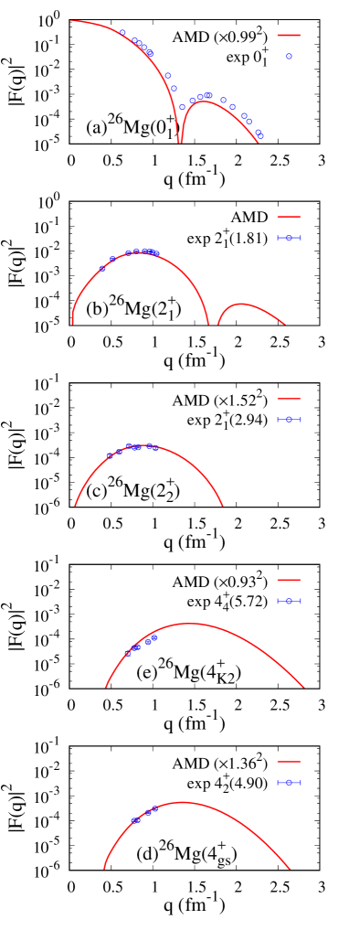
Figure 2: Charge form factors of ${}^{26}\textrm{Mg}$. The inelastic form factors $F(q)$ obtained by AMD are renormalized by $f^{\textrm{tr}}_{p}$ given in Table 4. The results of the $0^{+}_{1}$, $2^{+}_{1}$, $2^{+}_{2}$, $4^{+}_{\textrm{gs}}$, and $4^{+}_{K2}$ states are compared with the experimental data Lees1974 of the $0^{+}_{1}$, $2^{+}_{1}$(1.81 MeV), $2^{+}_{2}$(2.94 MeV), $4^{+}_{2}$(4.90 MeV), and $4^{+}_{4}$(5.72 MeV) states, respectively.

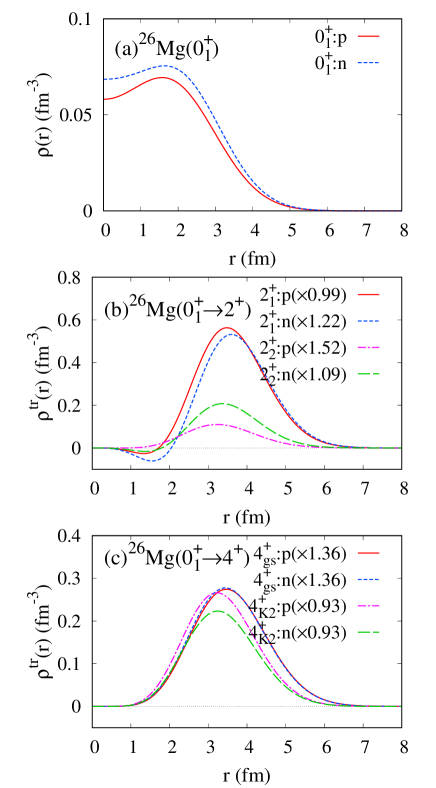
Figure 3: Proton and neutron diagonal and transition densities of ${}^{26}\textrm{Mg}$. (a) The diagonal densities of the $0^{+}_{1}$ state. (b) The renormalized transition densities from the $0^{+}_{1}$ state to the $2^{+}_{1}$ and $2^{+}_{2}$ states. (c) The renormalized transition densities from the $0^{+}_{1}$ state to the $4^{+}_{\textrm{gs}}$ and $4^{+}_{K2}$ states.

IV.2 ${}^{26}\textrm{Mg}+p$ and ${}^{26}\textrm{Mg}+\alpha$ reactions

Using the AMD densities of ${}^{26}\textrm{Mg}$, we perform the MCC calculations of $p$ scattering at $E_{p}=24$, 40, 60, and 100 MeV and $\alpha$ scattering at $E_{\alpha}=104$, 120, and 400 MeV. For coupled channels, we take into account the $0^{+}_{1}$, $2^{+}_{1}$, $2^{+}_{2}$, $4^{+}_{\textrm{gs}}$, and $4^{+}_{K2}$ states and $\lambda=2$ and 4 transitions between them. To see coupled channel (CC) effects, we also calculate one-step cross sections with distorted wave Born approximation (DWBA). The experimental excitation energies of the $0^{+}_{1}$, $2^{+}_{1}$, $2^{+}_{2}$, $4^{+}_{2}$, and $4^{+}_{4}$ states are used in the reaction calculations. For the transitions of $2^{+}_{1}\to 0^{+}_{1}$, $4^{+}_{\textrm{gs}}\to 0^{+}_{1}$, $2^{+}_{2}\to 0^{+}_{1}$, and $4^{+}_{K2}\to 0^{+}_{1}$, the renormalized transition densities are used as explained previously. For other transitions, we use theoretical transition densities without renormalization.

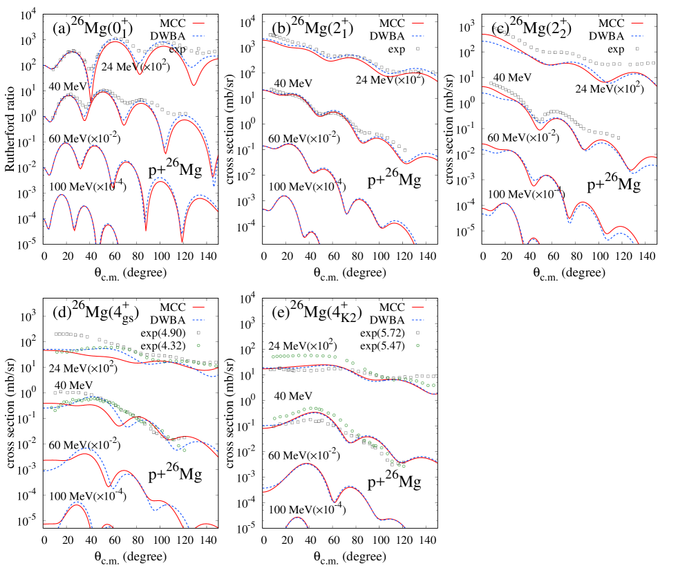
Figure 4: Cross sections of $p$ elastic and inelastic scattering off ${}^{26}\textrm{Mg}$ at $E_{p}=24$, 40, 60, and 100 MeV. The results obtained by the MCC and DWBA calculations are shown by red solid and blue dashed lines, respectively. Experimental data are cross sections at $E_{p}=24$ MeV Alons:1981rrm and $40$ MeV Zwieglinski:1983zz . The panels (a), (b), and (c) show the calculated and experimental cross sections of the $0^{+}_{1}$, $2^{+}_{1}$, and $2^{+}_{2}$ states, respectively. The panel (d) shows the calculated $4^{+}_{\textrm{gs}}$ cross sections together with the data observed for the $4^{+}_{2}$(4.90 MeV) and $4^{+}_{1}$(4.32 MeV) states. The panel (e) shows the calculated $4^{+}_{K2}$ cross sections compared with the data observed for the $4^{+}_{4}$(5.47 MeV) and $4^{+}_{3}$(5.72 MeV) states.

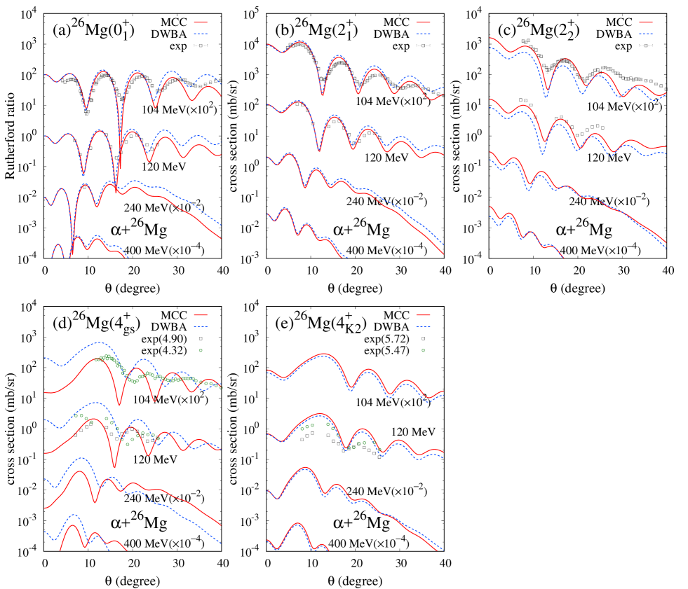
Figure 5: Same as Fig. 4 but for $\alpha$ scattering at $E_{\alpha}=104$, 120, 240, and 400 MeV. Experimental data at $E_{\alpha}=104$ MeV Rebel:1972nip and $E_{\alpha}=120$ MeV VanDerBorg:1981qiu are shown.

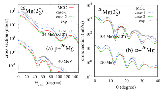
Figure 6: $2^{+}_{2}$ cross sections of the ${}^{26}\textrm{Mg}+p$ and ${}^{26}\textrm{Mg}+\alpha$ reactions calculated by MCC using the renormalized transition densities with the default, case-1, and case-2 scaling. (a) ($p,p^{\prime})$ cross sections at $E_{p}=24$ and $40$ MeV and (b) $(\alpha,\alpha^{\prime})$ cross sections at $E_{\alpha}=104$ and $120$ MeV. The experimental data of $(p,p^{\prime})$ are from Refs. Alons:1981rrm ; Zwieglinski:1983zz , those of $(\alpha,\alpha^{\prime})$ are from Refs. Rebel:1972nip ; VanDerBorg:1981qiu .

The MCC and DWBA results of the ${}^{26}\textrm{Mg}+p$ reaction are shown in Fig. 4 together with the experimental cross sections at $E_{p}=24$ and 40 MeV, and those of the ${}^{26}\textrm{Mg}+\alpha$ reaction are shown in Fig. 5 with the experimental cross sections at $E_{\alpha}=104$ and 120 MeV. As shown in Fig. 4(a), the MCC calculation reproduces well the $p$ elastic cross sections at $E_{p}=24$ and 40 MeV. It should be commented that spin-orbit interaction, which is omitted in the present reaction calculation, may smear the deep dip structure of the calculated cross sections. The calculation also describes the experimental data of $\alpha$ elastic scattering at $E_{\alpha}=104$ and 120 MeV (Fig. 5(a)).

For the ground-band $2^{+}_{1}$ state, the MCC calculation successfully reproduces the amplitudes and also the diffraction patterns of the $(p,p^{\prime})$ and $(\alpha,\alpha^{\prime})$ cross sections. For the inelastic scattering to the side-band $2^{+}_{2}$ state, the calculation reasonably describes the $(\alpha,\alpha^{\prime})$ data but somewhat underestimates the $(p,p^{\prime})$ data. Comparing the DWBA and MCC results, one can see that CC effects are minor in the $2^{+}_{1}$ and $2^{+}_{2}$ cross sections of $p$ scattering and $2^{+}_{1}$ cross sections of $\alpha$ scattering but give a significant contribution to the $2^{+}_{2}$ cross sections of low-energy $\alpha$ scattering.

For the $4^{+}_{\textrm{gs}}$ and $4^{+}_{K2}$ states, agreements with the experimental $(p,p^{\prime})$ cross sections are not enough satisfactory to discuss whether the present assignment of $4^{+}$ states is reasonable (Fig. 4(d) and Fig. 4(e)). For the $(\alpha,\alpha^{\prime})$ processes, the experimental cross sections observed for the $4^{+}_{2}$(4.90 MeV) state are reproduced well by the MCC result, which shows large suppression by the CC effect (Fig. 5(d)). For the $4^{+}_{K2}$ cross sections, the MCC calculation obtains almost no suppression by the CC effect and significantly overestimates the $(\alpha,\alpha^{\prime})$ data for the $4^{+}_{4}$(5.72 MeV) states. We can state that $p$ and $\alpha$ inelastic processes to low-lying $4^{+}$ states are not as simple as a theoretical description with the $4^{+}_{\textrm{gs}}$ and $4^{+}_{K2}$ states. Instead, they may be affected by significant state mixing and channel coupling, which are beyond the present AMD calculation. This indication is consistent with the $\gamma$ decay properties.

Let us discuss isospin properties of the $2^{+}_{1}$ and $2^{+}_{2}$ states with further detailed analysis of the inelastic cross sections. As shown previously, the MCC calculation gives good reproduction of the $2^{+}_{1}$ cross sections in describing the peak and dip structures of the $(p,p^{\prime})$ data at $E_{p}=40$ MeV and $(\alpha,\alpha^{\prime})$ data at $E_{\alpha}$=120 MeV (Fig. 4(b) and Fig. 5(b)). For the $2^{+}_{2}$ state, it describes the diffraction patterns of the $(p,p^{\prime})$ data but somewhat underestimates absolute amplitudes of the cross sections. In order to discuss possible uncertainty in the neutron strength (or the $M_{n}/M_{p}$ ratio) of the $0^{+}_{1}\to 2^{+}_{2}$ transition, we consider here optional choices of the renormalization of the transition densities by changing the scaling factors ($f^{\textrm{tr}}_{p}$,$f^{\textrm{tr}}_{n}$) for this transition from the default values $(f^{\textrm{tr}}_{p},f^{\textrm{tr}}_{n})=(1.52,1.09)$. The values of $(f^{\textrm{tr}}_{p},f^{\textrm{tr}}_{n})$, $M_{p}$, $M_{n}$, and $M_{n}/M_{p}$ for these two choices are listed in Table 4. In the case-1, we choose the same scaling for the proton and neutron parts as $(f^{\textrm{tr}}_{p},f^{\textrm{tr}}_{n})=(1.52,1.52)$. In this case, the neutron transition density is enhanced by 40% from the default MCC calculation (the neutron transition strengths is enhanced by a factor of two). The case-2 choice is $(f^{\textrm{tr}}_{p},f^{\textrm{tr}}_{n})=(2.20,0.83)$, which corresponds to an assumption of the isoscalar transition $M_{p}=M_{n}$ keeping the isoscalar component $M_{p}+M_{n}$ unchanged. In these two optional cases, other transitions are the same as the default calculation. In Fig. 6, we show the $2^{+}_{2}$ cross sections obtained by MCC with the case-1 and case-2 choices. In the case-1 calculation, one can see that the 40% increase of the neutron transition density significantly enhances the $(p,p^{\prime})$ cross sections and slightly raises the $(\alpha,\alpha^{\prime}$) cross sections. As a result, the calculation well reproduces the $(p,p^{\prime})$ cross sections, in particular, at $E_{p}=40$ MeV and also obtains a better result for the $(\alpha,\alpha^{\prime})$ cross sections. In the case-2 calculation (isoscalar assumption), the result for $(p,p^{\prime})$ cross sections becomes somewhat worse, and that for $(\alpha,\alpha^{\prime})$ cross sections is unchanged. This result indicates that the $(p,p^{\prime})$ process sensitively probes the dominant neutron component of the $0^{+}_{1}\to 2^{+}_{2}$ transition and the $(\alpha,\alpha^{\prime})$ process can probe the isoscalar component as expected. In the present analysis, the case-1 calculation is favored to describe the $2^{+}_{2}$ cross sections in both the $(p,p^{\prime})$ and $(\alpha,\alpha^{\prime})$ processes. This analysis supports the case-1 prediction for the $0^{+}_{1}\to 2^{+}_{2}$ transition of the neutron transition matrix $M_{n}\sim 8$ fm² (the squared ratio $|M_{n}/M_{p}|^{2}\sim 7$).

IV.3 Transition properties of ${}^{10}\textrm{Be}$

For ${}^{10}\textrm{Be}$, experimental information of $B(E\lambda)$ is limited. For the transition from the $0^{+}_{1}$ state, the available data are the observed values of $B(E2;2^{+}_{1}\to 0^{+}_{1})$ and its mirror transition, with which we adjust the scaling factors of the renormalization. The transition matrix elements ($M_{p}$ and $M_{n}$) and the scaling factors ($f^{\textrm{tr}}_{p}$ and $f^{\textrm{tr}}_{p}$) of $2^{+}_{1}\to 0^{+}_{1}$ in ${}^{10}\textrm{Be}$ are given in Table 4. Theoretical values before and after the renormalization are shown together with the experimental values used for fitting. For other transitions, theoretical transition densities without the renormalization are used for the MCC calculation.

Figure 7 shows calculated diagonal densities of ${}^{10}\textrm{Be}$. Compared to the ground state, the $0^{+}_{2}$($K^{\pi}=0^{+}_{2}$) and $1^{-}_{1}$($K^{\pi}=1^{-}$) states show longer tails of the proton and neutron diagonal densities because of the developed cluster structures.

The transition densities of ${}^{10}\textrm{Be}$ are shown in Fig. 8. Let us compare $2^{+}$ transitions from the $0^{+}_{1}$ state to the $2^{+}_{1}$($K^{\pi}=0^{+}_{1}$), $2^{+}_{2}$($K^{\pi}=2^{+}$), and $2^{+}_{3}$($K^{\pi}=0^{+}_{2}$) states. In the ground-band transition, $0^{+}_{1}\to 2^{+}_{1}$, the neutron transition density is similar to the proton one because this transition is the isoscalar excitation constructed by the $K=0$ rotation of the $2\alpha$ core part. In other transitions, the amplitude of the neutron transition density is more than twice larger than that of the proton one showing the neutron dominance in the $2^{+}_{2}$ and $2^{+}_{3}$ excitations. Absolute amplitude of the neutron transition density is strongest in the ground-band $0^{+}_{1}\to 2^{+}_{1}$ transition, smaller in $0^{+}_{1}\to 2^{+}_{2}$, and further smaller in $0^{+}_{1}\to 2^{+}_{3}$. One of the striking features is that, in the side-band transition, $0^{+}_{1}\to 2^{+}_{2}$, the proton component is opposite (negative sign) to the neutron one and gives cancellation effect to the isoscalar component, while the proton and neutron components are coherent in the $2^{+}_{1}$ and $2^{+}_{3}$ excitations. In the radial behavior of the neutron transition density, one can see that the $0^{+}_{1}\to 2^{+}_{2}$ transition has a peak amplitude slightly shifted inward compared with $0^{+}_{1}\to 2^{+}_{1}$ but the difference is not so remarkable. On the other hand, the $0^{+}_{1}\to 2^{+}_{3}$ transition has amplitude shifted to the outer region.

In other inelastic transitions to the $0^{+}_{2}$, $1^{-}_{1}$, and $3^{-}_{1}$ states, the neutron transition density is dominant while the proton transition density is relatively weak indicating the neutron dominance. It should be commented that the $0^{+}_{1}\to 0^{+}_{2}$ and $0^{+}_{1}\to 1^{-}_{1}$ transitions show nodal structures as expected from the usual behavior of monopole and dipole transitions.

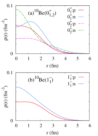
Figure 7: Diagonal densities of ${}^{10}\textrm{Be}$. The proton and neutron densities of the (a) $0^{+}_{1,2}$ and (b) $1^{-}_{1}$ states.

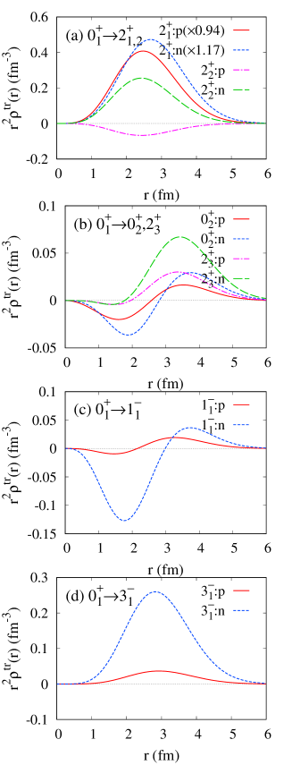
Figure 8: Transition densities of ${}^{10}\textrm{Be}$. The proton and neutron transition densities from the $0^{+}_{1}$ state to the (a) $2^{+}_{1,2}$, (b) $0^{+}_{2}$, $2^{+}_{3}$, (c) $1^{-}_{1}$, and (d) $3^{-}_{1}$ states. The $0^{+}_{1}\to 2^{+}_{1}$ transition densities are renormalized ones.

IV.4 ${}^{10}\textrm{Be}+p$ and ${}^{10}\textrm{Be}+\alpha$ reactions

Using the AMD densities of ${}^{10}\textrm{Be}$, we perform the MCC calculations of the ${}^{10}\textrm{Be}+p$ and ${}^{10}\textrm{Be}+\alpha$ reactions. For the coupled channels, we adopt the $0^{+}_{1,2}$, $2^{+}_{1.2.3}$, $1^{-}_{1}$, and $3^{-}_{1}$ states with $\lambda=0$, 1, 2, and 3 transitions between them. The experimental excitation energies of ${}^{10}\textrm{Be}$ are used. For the $2^{+}_{1}\to 0^{+}_{1}$ transition, the renormalized transition densities are used as explained previously. One-step (DWBA) cross sections are also calculated for comparison. We also calculate the ${}^{10}\textrm{C}+p$ and ${}^{10}\textrm{C}+\alpha$ reactions assuming the mirror symmetry of diagonal and transition densities between the proton and neutron parts in the $A=10$ systems. Coulomb shifts of excitation energies are omitted.

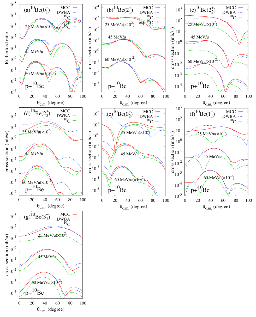
Figure 9: Elastic and inelastic cross sections of the ${}^{10}\textrm{Be}+p$ and ${}^{10}\textrm{C}+p$ reactions at $E=25$, 45, 60, and 100 MeV/u. The MCC and DWBA results of ${}^{10}\textrm{Be}+p$ are shown by red solid and blue dashed lines, respectively. The MCC results of ${}^{10}\textrm{C}+p$ are shown by green long-dashed lines. The experimental ${}^{10}\textrm{Be}+p$ elastic cross sections at $E=58.4$ MeV/u CortinaGil:1997zk are shown by red squares in the panel (a). The experimental ${}^{10}\textrm{C}+p$ cross sections at $E=45$ MeV/u Jouanne:2005pb observed for the $0^{+}_{1}$ and $2^{+}_{1}$ states are shown by blue circles in the panels (a) and (b).

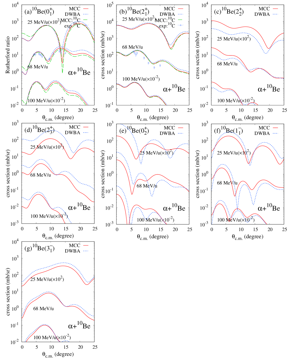
Figure 10: Calculated elastic and inelastic cross sections of ${}^{10}\textrm{Be}+\alpha$ at $E=25$, 68, and 100 MeV/u. The MCC and DWBA cross sections are shown by red solid and blue dashed lines, respectively. In the panels (a) and (b), the calculated cross sections of ${}^{10}\textrm{C}+\alpha$ are shown by green dashed lines compared with the experimental cross sections at $E=68$ MeV/u from Ref. Furuno:2019lyp .

Figure 9 shows the calculated cross sections of ${}^{10}\textrm{Be}+p$ at $E=25$, 45, and 60 MeV/u together with those of ${}^{10}\textrm{C}+p$, and Fig. 10 shows the results of ${}^{10}\textrm{Be}+\alpha$ at $E=25$, 68, and 100 MeV/u. In Figs. 9(a) and (b), the results are compared with the experimental ${}^{10}\textrm{Be}+\alpha$ data of the elastic cross sections at $E=60$ MeV/u CortinaGil:1997zk and the ${}^{10}\textrm{C}+p$ data of the elastic and $2^{+}_{1}$ cross sections at $E=45$ MeV/u Jouanne:2005pb , which have been observed by the inverse kinematics experiments. The MCC calculations well reproduce those data as already shown in our previous work Kanada-Enyo:2019uvg . It should be noted again that the dip structure of elastic scattering can be smeared by the spin-orbit interaction omitted in the present calculation. In Figs. 10(a) and (b), we also show the result of the ${}^{10}\textrm{C}+\alpha$ reaction compared with the ${}^{10}\textrm{C}+\alpha$ data at $E=68$ MeV/u, which have been recently measured by the inverse kinematics experiment Furuno:2019lyp . The observed data of the elastic and $2^{+}_{1}$ cross sections tend to be smaller than the present result. Comparing the MCC and DWBA results, one can see that CC effects are not minor except for the $2^{+}_{1}$ and $3^{-}_{1}$ cross sections of ${}^{10}\textrm{Be}+p$ and the $2^{+}_{1}$ cross sections of ${}^{10}\textrm{Be}+\alpha$. At low incident energies, remarkable CC effects can be seen in the $0^{+}_{2}$ cross sections of ${}^{10}\textrm{Be}+p$ and the $2^{+}_{2}$, $2^{+}_{3}$, and $0^{+}_{2}$ cross sections of ${}^{10}\textrm{Be}+\alpha$. The CC effects enhance the $2^{+}_{2}$ cross sections and suppress the $0^{+}_{2}$ and $2^{+}_{3}$ cross sections. At higher incident energies, the CC effects become weaker but they remain to be significant at forward angles even at $E=60$ MeV/u of ${}^{10}\textrm{Be}+p$ and $E=100$ MeV/u of ${}^{10}\textrm{Be}+\alpha$.

Let us compare ${}^{10}\textrm{Be}+p$ and ${}^{10}\textrm{C}+p$ cross sections. If a transition has the isoscalar character, difference between ${}^{10}\textrm{Be}+p$ and ${}^{10}\textrm{C}+p$ cross sections should be small. On the other hand, in the neutron dominant case, it is naively expected that ${}^{10}\textrm{Be}+p$ cross sections are enhanced and ${}^{10}\textrm{C}+p$ cross sections are relatively suppressed because the $p$ scattering sensitively probes the neutron component rather than the proton component. In Fig. 9, the ${}^{10}\textrm{C}+p$ cross sections (green dashed lines) are compared with the ${}^{10}\textrm{Be}+p$ cross sections (red solid lines). As expected, the difference is small in the $2^{+}_{1}$ cross sections, because of the isoscalar nature of the ground-band transition. On the other hand, for the $2^{+}_{2}$, $1^{-}_{1}$, and $3^{-}_{1}$ states, the ${}^{10}\textrm{C}+p$ cross sections are remarkably suppressed compared with the ${}^{10}\textrm{Be}+p$ cross sections because of the neutron dominant characters of these transitions in ${}^{10}\textrm{Be}$ (the proton dominance in ${}^{10}\textrm{C}$).

For quantitative discussions, we compare the integrated cross sections of the inelastic scattering of the ${}^{10}\textrm{Be}+p$, ${}^{10}\textrm{C}+p$ and ${}^{10}\textrm{Be}+\alpha$ reactions. Figure 11 shows the MCC results of the cross sections at $E=25,$ 60, and 100 MeV/u. For the $2^{+}_{1}$ cross sections, one can see only a small difference between ${}^{10}\textrm{Be}+p$ and ${}^{10}\textrm{C}+p$. This is a typical example of the isoscalar excitation and can be regarded as reference data to be compared with other excitations. For the side-band $2^{+}_{2}$ sate, the difference between ${}^{10}\textrm{Be}+p$ and ${}^{10}\textrm{C}+p$ is huge as one order of the magnitude of the cross sections because of the cancellation between proton and neutron components in the ${}^{10}\textrm{C}+p$ reaction. As shown in the transition densities (Fig. 8(a)) and the matrix elements (Table 3) of ${}^{10}\textrm{Be}$, the proton component of the $2^{+}_{2}$ transition in ${}^{10}\textrm{Be}$ is weak but opposite sign to the neutron one, and it gives the strong cancellation in the mirror transitions probed by the ${}^{10}\textrm{C}+p$ reaction. It also gives some cancellation in the isoscalar component probed by the ${}^{10}\textrm{Be}+\alpha$ reaction, but the cancellation is tiny in the ${}^{10}\textrm{Be}+p$ reaction. The difference of the production rates between the ${}^{10}\textrm{Be}+p$ and ${}^{10}\textrm{C}+p$ reactions is also large in the $3^{-}_{1}$ cross section as expected from its remarkable neutron dominance (the ratio $M_{n}/M_{p}=6.4$). Namely, the $3^{-}_{1}$ cross sections in the ${}^{10}\textrm{Be}+p$ reaction are largely enhanced compared to the ${}^{10}\textrm{C}+p$ reaction. Similarly, the enhancement of the ${}^{10}\textrm{Be}+p$ cross sections is also obtained for the $0^{+}_{2}$ and $2^{+}_{3}$ states in the $K^{\pi}=0^{+}_{2}$ cluster-band, but it is not so remarkable as the $3^{-}_{1}$ state ($M_{n}/M_{p}=6.4$) because of their weaker neutron dominance ($M_{n}/M_{p}=1.89$ of $0^{+}_{1}\to 0^{+}_{2}$ and $M_{n}/M_{p}=2.5$ of $0^{+}_{1}\to 2^{+}_{3}$). It is rather striking that, the difference in the $1^{-}_{1}$ production rates between ${}^{10}\textrm{Be}+p$ and ${}^{10}\textrm{C}+p$ is unexpectedly large even though the neutron dominance of the $1^{-}_{1}$ state is weaker as $M_{n}/M_{p}=1.46$ than the $2^{+}_{3}$ and $0^{+}_{2}$ states. This is understood by the difference in radial behaviors of the proton and neutron transition densities. As shown in Fig. 8(c) for the $0^{+}_{1}\to 1^{-}_{1}$ transition densities, the neutron amplitude is dominant in the outer region and enhances the ${}^{10}\textrm{Be}+p$ cross sections. Moreover, at the surface region of $r=2$–3 fm, the proton transition density is opposite to the neutron one and gives the cancellation effect in the ${}^{10}\textrm{C}+p$ reaction.

In the experimental side, the $(p,p^{\prime})$ and $(\alpha,\alpha^{\prime})$ cross sections off ${}^{10}\textrm{Be}$ and ${}^{10}\textrm{C}$ have been measured only for the $2^{+}_{1}$ state. Indeed, according to the present calculation, the $2^{+}_{1}$ state is strongly populated in $p$ and $\alpha$ inelastic scattering processes, but other states are relatively weak as more than one order smaller cross sections than the $2^{+}_{1}$ state. Below, we discuss sensitivity of the ${}^{10}\textrm{Be}+p$, ${}^{10}\textrm{Be}+\alpha$, and ${}^{10}\textrm{C}+p$ reactions to observe higher excited states above the $2^{+}_{1}$ state.

Firstly, we examine the integrated cross sections and discuss the production rates of excited states and their projectile and energy dependencies. In Figs. 11(b)-(f), 7%–10% of the $2^{+}_{1}$ cross sections of the ${}^{10}\textrm{Be}+p$ and ${}^{10}\textrm{Be}+\alpha$ reactions are shown by light-green and pink shaded areas, respectively. We consider these areas as references of one-order smaller magnitude of the $2^{+}_{1}$ cross sections for comparison. For the side-band $2^{+}_{2}$ transition (Fig. 11(b)), the ${}^{10}\textrm{Be}+p$ cross sections (blue dashed line) exceed the 7%–10% area (light-green) indicating that the ${}^{10}\textrm{Be}+p$ reaction can be an efficient tool to observe the neutron dominance of the $2^{+}_{2}$ excitation. Also the ${}^{10}\textrm{Be}+\alpha$ cross sections (red solid lines) reach 10% of the $2^{+}_{1}$ cross sections at $E=25$ MeV/u but decrease at high energies. For the $3^{-}_{1}$ transitions (Fig. 11(f)), the ${}^{10}\textrm{Be}+p$ cross sections (blue dashed line) are within the 7%–10% area (light-green), and the ${}^{10}\textrm{Be}+\alpha$ cross sections are approximately 5% of the $2^{+}_{1}$ cross sections. For other states, the population is much weaker as 1–2% of the $2^{+}_{1}$ state or less.

Next, we compare the $0^{+}_{2}$, $2^{+}_{2}$, and $1^{-}_{1}$ cross sections of each reaction. Since these three states almost degenerate around $E_{x}\approx 6$ MeV in the experimental energy spectra, it may be difficult to resolve observed cross sections to individual states. In Figs. 12(a), (b), and (c), the calculated cross sections of ${}^{10}\textrm{Be}+p$ at $E$=60 MeV/u, ${}^{10}\textrm{C}+p$ at $E$=60 MeV/u, and ${}^{10}\textrm{Be}+\alpha$ at $E$=68 MeV/u are shown, respectively. The cross sections of each state and the incoherent sum of three states are plotted. In the ${}^{10}\textrm{Be}+p$ reaction, the $2^{+}_{2}$ cross sections dominate the summed cross sections while the $0^{+}_{2}$ and $1^{-}_{1}$ contributions are minor. In the ${}^{10}\textrm{C}+p$ reaction, where the $2^{+}_{2}$ cross sections are strongly suppressed, the magnitude of the $0^{+}_{2}$ cross sections is comparable to that of $2^{+}_{2}$ in the $\theta_{\textrm{c.m.}}=20$–$40^{\circ}$ range, and the $1^{-}_{1}$ state gives major contribution at $\theta_{\textrm{c.m.}}\sim 50^{\circ}$ and smears the second dip of the $2^{+}_{2}$ cross sections in the summed cross sections. In the ${}^{10}\textrm{Be}+\alpha$ reaction at forward angles, the $0^{+}_{2}$ and $1^{-}_{1}$ contributions are minor compared to the dominant $2^{+}_{2}$ contribution. It seems to contradict the usual expectation that forward angle $\alpha$ scattering can be generally useful to observe monopole transitions. But it is not the case in the ${}^{10}\textrm{Be}+\alpha$ reaction because the $0^{+}_{2}$ cross sections at forward angles are strongly suppressed by the CC effect. Alternatively, detailed analysis of ${}^{10}\textrm{C}+p$ cross sections in a wide range of scattering angles may be promising to observe the $0^{+}_{2}$ and $1^{-}_{1}$ states.

It should be commented that the predicted cross sections still contain structure model ambiguity, in particular, for the cluster-bands. Basis configurations adopted in the present AMD calculation are not enough to describe details of the inter-cluster motion, which may somewhat enhance the monopole transition strengths.

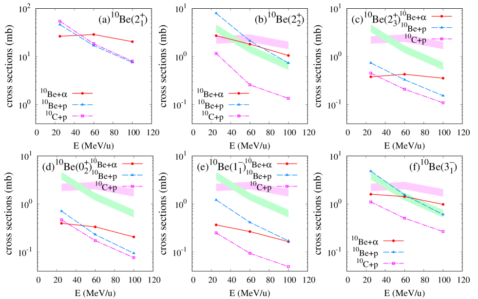
Figure 11: Integrated cross sections of ${}^{10}\textrm{Be}+p$, ${}^{10}\textrm{C}+p$, and ${}^{10}\textrm{Be}+\alpha$ inelastic processes are shown by (blue) triangles, (magenta) squares, and (red) circles, respectively. The cross sections at $E=25$, 60, and 100 MeV/u are calculated with MCC. In panels for the (b) $2^{+}_{2}$, (c) $2^{+}_{3}$, (d) $0^{+}_{2}$, (e) $1^{-}_{1}$, and (f) $3^{-}_{1}$ states, 7%–10% of the $2^{+}_{1}$ cross sections of the ${}^{10}\textrm{Be}+p$ and ${}^{10}\textrm{Be}+\alpha$ reactions are shown by light-green and pink shaded areas, respectively, as references.

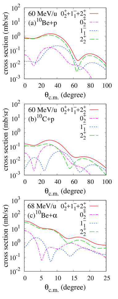
Figure 12: The $0^{+}_{2}$, $1^{-}_{1}$, and $2^{+}_{2}$ cross sections of the ${}^{10}\textrm{Be}+p$, ${}^{10}\textrm{C}+p$, and ${}^{10}\textrm{Be}+\alpha$ reactions obtained by the MCC calculations. (a)${}^{10}\textrm{Be}+p$ at $E=60$ MeV/u, (b)${}^{10}\textrm{C}+p$ at $E=60$ MeV/u, and (c)${}^{10}\textrm{Be}+\alpha$ at $E=68$ MeV/u. The $0^{+}_{2}$, $1^{-}_{1}$, and $2^{+}_{2}$ cross sections and their incoherent sum are shown by magenta dot-dashed, blue dashed, green long dashed, and red solid lines.

V Summary

Isospin characters of nuclear excitations in ²⁶Mg and ¹⁰Be were investigated with the MCC calculations of $p$ and $\alpha$ inelastic scattering. The structure calculations of ²⁶Mg and ¹⁰Be were done by antisymmetrized molecular dynamics (AMD). In the AMD calculations, the $K^{\pi}=0^{+}$ ground- and $K^{\pi}=2^{+}$ side-bands were obtained in ²⁶Mg and ¹⁰Be. In both systems, the ground-band $2^{+}_{1}$($K^{\pi}=0^{+}_{1}$) state and the side-band $2^{+}_{2}$($K^{\pi}=2^{+}$) state have quite different isospin characters. The former has the isoscalar feature and the latter shows the neutron dominance character. This can be a general feature in $N=Z+2$ system having a prolately deformed $N=Z$ core surrounded by valence neutrons.

The MCC calculations of $p$ and $\alpha$ inelastic scattering off ²⁶Mg and ¹⁰Be were performed with the Melbourne $g$-matrix folding approach by using the matter and transition densities of the target nuclei calculated with AMD. The calculations reasonably reproduced the observed $0^{+}_{1}$, $2^{+}_{1}$, and $2^{+}_{2}$ cross sections of ²⁶Mg+$p$ scattering at $E_{p}=24$ and 40 MeV and of ²⁶Mg+$\alpha$ scattering at $E_{\alpha}=104$ and 120 MeV. It was shown that the ²⁶Mg+$p$ scattering is a sensitive probe to the neutron component of the $0^{+}_{1}\to 2^{+}_{2}$ transition. In the present analysis, the neutron transition matrix element $M_{n}\sim 8$ fm² (the squared ratio $|M_{n}/M_{p}|^{2}\sim 7$) of the $0^{+}_{1}\to 2^{+}_{2}$ transitions in ${}^{26}\textrm{Mg}$ is favored to reproduce the ${}^{26}\textrm{Mg}+p$ and ${}^{26}\textrm{Mg}+\alpha$ cross sections consistently.

For ¹⁰Be+$p$ and ¹⁰Be+$\alpha$ scattering, inelastic cross sections to the excited states in the $K^{\pi}=0^{+}_{1}$ ground-, $K^{\pi}=2^{+}$ side-, $K^{\pi}=0^{+}_{2}$ cluster-, and $K^{\pi}=1^{-}$ cluster-bands were discussed. In a comparison of the ${}^{10}\textrm{Be}+p$, ${}^{10}\textrm{C}+p$, and ${}^{10}\textrm{Be}+\alpha$ reactions, the isospin characters of transitions in inelastic scattering processes were investigated. Also in ${}^{10}\textrm{Be}$, the $p$ inelastic scattering was found to be a sensitive probe to the neutron dominance in the $2^{+}_{2}$ excitation. The significant suppression of the $2^{+}_{2}$ cross sections of ${}^{10}\textrm{C}+p$ was obtained because of the cancellation of the proton and neutron components in the transition. The present prediction of the inelastic scattering off ${}^{10}\textrm{Be}$ may be useful for the feasibility test of future experiments in the inverse kinematics.

- (1) A. M. Bernstein, V. R. Brown and V. A. Madsen, Phys. Lett. 71B, 48 (1977).
- (2) A. M. Bernstein, V. R. Brown and V. A. Madsen, Phys. Rev. Lett. 42, 425 (1979).
- (3) A. M. Bernstein, V. R. Brown and V. A. Madsen, Phys. Lett. 103B, 255 (1981).
- (4) B. A. Brown and B. H. Wildenthal, Phys. Rev. C 21, 2107 (1980).
- (5) B. A. Brown et al., Phys. Rev. C 26, 2247 (1982).
- (6) T. K. Alexander, G. C. Ball, W. G. Davies, J. S. Forster, I. V. Mitchell and H.-B. Mak, Phys. Lett. 113B, 132 (1982).
- (7) C.-A. Wiedner, K. R. Cordell, W. Saathoff, S. T. Thornton, J. Bolger, E. Boschitz, G. Proebstle and J. Zichy, Phys. Lett. 97B, 37 (1980).
- (8) P. W. F. Alons, H. P. Blok, J. F. A. V. Hienen and J. Blok, Nucl. Phys. A 367, 41 (1981).
- (9) B. Zwieglinski, G. M. Crawley, J. A. Nolen and R. M. Ronningen, Phys. Rev. C 28, 542 (1983).
- (10) K. Van Der Borg, M. N. Harakeh and A. Van Der Woude, Nucl. Phys. A 365, 243 (1981).
- (11) Y. Kanada-En’yo and H. Horiuchi, Phys. Rev. C 55, 2860 (1997).
- (12) H. Iwasaki et al., Phys. Lett. B 481, 7 (2000).
- (13) Y. Kanada-En’yo, Phys. Rev. C 71, 014310 (2005).
- (14) Y. Kanada-En’yo, Phys. Rev. C 71, 014303 (2005).
- (15) H. Sagawa, X. R. Zhou, X. Z. Zhang and T. Suzuki, Phys. Rev. C 70, 054316 (2004).
- (16) M. Takashina, Y. Kanada-En’yo and Y. Sakuragi, Phys. Rev. C 71, 054602 (2005).
- (17) H. J. Ong et al., Phys. Rev. C 73, 024610 (2006).
- (18) T. J. Burvenich, W. Greiner, L. Guo, P. Klupfel and P. G. Reinhard, J. Phys. G 35, 025103 (2008).
- (19) M. Takashina and Y. Kanada-En’yo, Phys. Rev. C 77, 014604 (2008).
- (20) Z. Elekes, N. Aoi, Z. Dombradi, Z. Fulop, T. Motobayashi and H. Sakurai, Phys. Rev. C 78, 027301 (2008).
- (21) M. Wiedeking et al., Phys. Rev. Lett. 100, 152501 (2008).
- (22) J. M. Yao, J. Meng, P. Ring, Z. X. Li, Z. P. Li and K. Hagino, Phys. Rev. C 84, 024306 (2011).
- (23) C. Forssén, R. Roth and P. Navrátil, J. Phys. G 40, 055105 (2013).
- (24) T. Furuno et al., Phys. Rev. C 100, no. 5, 054322 (2019).
- (25) W. von Oertzen, M. Freer and Y. Kanada-En’yo, Phys. Rep. 432, 43 (2006).
- (26) Y. Kanada-En’yo, M. Kimura and A. Ono, Prog.. Theor. Exp. Phys. 2012, 01A202 (2012).
- (27) M. Ito and K. Ikeda, Rep. Prog. Phys. 77, 096301 (2014).
- (28) Y. Kanada-En’yo, Phys. Rev. C 84, 024317 (2011).
- (29) K. Amos, P. J. Dortmans, H. V. von Geramb, S. Karataglidis, and J. Raynal, Adv. Nucl. Phys. 25, 275 (2000).
- (30) S. Karataglidis, Y. J. Kim and K. Amos, Nucl. Phys. A 793, 40 (2007).
- (31) K. Minomo, K. Ogata, M. Kohno, Y. R. Shimizu and M. Yahiro, J. Phys. G 37, 085011 (2010).
- (32) M. Toyokawa, K. Minomo and M. Yahiro, Phys. Rev. C 88, no. 5, 054602 (2013).
- (33) K. Minomo, K. Washiyama and K. Ogata, arXiv:1712.10121 [nucl-th].
- (34) K. Egashira, K. Minomo, M. Toyokawa, T. Matsumoto and M. Yahiro, Phys. Rev. C 89, 064611 (2014).
- (35) K. Minomo and K. Ogata, Phys. Rev. C 93, 051601(R) (2016).
- (36) Y. Kanada-En’yo and K. Ogata, Phys. Rev. C 99, no. 6, 064601 (2019).
- (37) Y. Kanada-En’yo and K. Ogata, Phys. Rev. C 99, no. 6, 064608 (2019).
- (38) Y. Kanada-En’yo and K. Ogata, Phys. Rev. C 100, no. 6, 064616 (2019).
- (39) Y. Kanada-En’yo and K. Ogata, arXiv:2002.02625 [nucl-th].
- (40) Y. Kanada-En’yo, H. Horiuchi and A. Ono, Phys. Rev. C 52, 628 (1995).
- (41) Y. Kanada-En’yo, Phys. Rev. Lett. 81, 5291 (1998).
- (42) Y. Kanada-En’yo, H. Horiuchi and A. Dote, Phys. Rev. C 60, 064304 (1999).
- (43) T. Ando, K.Ikeda, and A. Tohsaki, Prog. Theor. Phys. 64, 1608 (1980).
- (44) R. Tamagaki, Prog. Theor. Phys. 39, 91 (1968).
- (45) N. Yamaguchi, T. Kasahara, S. Nagata, and Y. Akaishi, Prog. Theor. Phys. 62, 1018 (1979).
- (46) A Nagel et al., J. Phys. A 7, 1697 (1974).
- (47) J.L. Durell et al., J. Phys. A 5, 302 (1972).
- (48) M. S. Basunia and A. M. Hurst, Nucl. Data Sheets 134, 1 (2016).
- (49) D. R. Tilley, J. H. Kelley, J. L. Godwin, D. J. Millener, J. E. Purcell, C. G. Sheu and H. R. Weller, Nucl. Phys. A 745, 155 (2004).
- (50) I. Angeli and K. P. Marinova, At. Data Nucl. Data Tables 99, 69 (2013).
- (51) E W Lees, A Johnston, S W Brain, C S Currant, W A Gillespie and R P Singhal, J. Phys. A 7, 936 (1974).
- (52) B. A. Brown, A. Arima and J. B. McGrory, Nucl. Phys. A 277, 77 (1977).
- (53) H. Rebel, G. W. Schweimer, G. Schatz, J. Specht, R. Löhken, G. Hauser, D. Habs and H. Klewe-Nebenius, Nucl. Phys. A 182, 145 (1972).
- (54) M. D. Cortina-Gil et al., Phys. Lett. B 401, 9 (1997).
- (55) C. Jouanne et al., Phys. Rev. C 72, 014308 (2005).