Theoretical and Computable Optimal Subspace Expansions for Matrix Eigenvalue Problems

Abstract

Consider the optimal subspace expansion problem for the matrix eigenvalue problem $Ax=\lambda x$: Which vector $w$ in the current subspace $\mathcal{V}$, after multiplied by $A$, provides an optimal subspace expansion for approximating a desired eigenvector $x$ in the sense that $x$ has the smallest angle with the expanded subspace $\mathcal{V}_{w}=\mathcal{V}+{\rm span}\{Aw\}$, i.e., $w_{opt}=\arg\max_{w\in\mathcal{V}}\cos\angle(\mathcal{V}_{w},x)$? This problem is important as many iterative methods construct nested subspaces that successively expand $\mathcal{V}$ to $\mathcal{V}_{w}$. An expression of $w_{opt}$ by Ye (Linear Algebra Appl., 428 (2008), pp. 911–918) for $A$ general, but it could not be exploited to construct a computable (nearly) optimally expanded subspace. He turns to deriving a maximization characterization of $\cos\angle(\mathcal{V}_{w},x)$ for a given $w\in\mathcal{V}$ when $A$ is Hermitian. We generalize Ye’s maximization characterization to the general case and find its maximizer. Our main contributions consist of explicit expressions of $w_{opt}$, $(I-P_{V})Aw_{opt}$ and the optimally expanded subspace $\mathcal{V}_{w_{opt}}$ for $A$ general, where $P_{V}$ is the orthogonal projector onto $\mathcal{V}$. These results are fully exploited to obtain computable optimally expanded subspaces within the framework of the standard, harmonic, refined, and refined harmonic Rayleigh–Ritz methods. We show how to efficiently implement the proposed subspace expansion approaches. Numerical experiments demonstrate the effectiveness of our computable optimal expansions.

1 Introduction

Consider the large scale matrix eigenproblem $Ax=\lambda x$ with $A\in\mathcal{C}^{n\times n}$ and $\|x\|=1$, where $\|\cdot\|$ is the 2-norm of a vector or matrix. We are interested in an exterior eigenvalue $\lambda$ and the associated eigenvector $x$. A number of numerical methods have been available for solving this kind of problem [1, 14, 15, 21, 19]. Of them, Lanczos or Arnoldi type methods [1, 15, 19] are typical, and they are projection methods on the sequence of nested $k$-dimensional Krylov subspaces

$$\mathcal{V}_{k}=\mathcal{K}_{k}(A,v_{1})={\rm span}\{v_{1},Av_{1},\ldots,A^{k-1}v_{1}\}$$

and compute approximations to $\lambda$ and $x$. For $A$ Hermitian, Arnoldi type methods reduce to Lanczos type methods [1, 14]. Suppose that $V_{k}=(v_{1},\ldots,v_{k})$ is column orthonormal and is generated by the Lanczos process in the Hermitian case or the Arnoldi process in the non-Hermitian case, and take the expansion vector $w_{k}=v_{k}\in\mathcal{V}_{k}$. Then the next basis vector $v_{k+1}$ is obtained by orthonormalizing $Aw_{k}$ against $V_{k}$, the projection matrix $V_{k}^{H}AV_{k}$ of $A$ onto $\mathcal{V}_{k}$ is Hermitian tridiagonal for $A$ Hermitian or upper Hessenberg for $A$ non-Hermitian, and the columns of $(V_{k},v_{k+1})$ form an orthonormal basis of the $(k+1)$-dimensional Krylov subspace $\mathcal{V}_{k+1}$, where the superscript $H$ denotes the conjugate transpose of a vector or matrix. If the expansion vector $v_{k}$ in $Av_{k}$ is replaced by any $w_{k}\in\mathcal{V}_{k}$ that is not deficient in $v_{k}$, we deduce from Proposition 1 of Ye [25] that the same $\mathcal{V}_{k+1}$ and $V_{k+1}$ are generated.

However, if we start with a non-Krylov subspace $\mathcal{V}_{k}$, then the expanded subspace $\mathcal{V}_{k+1}$ critically depends on the choice of expansion vector $w_{k}\in\mathcal{V}_{k}$. It is well known that the success of a general projection method requires that an underlying subspace contain sufficiently accurate approximations to $x$ but a sufficiently accurate subspace cannot guarantee the convergence of the Ritz and harmonic Ritz vectors obtained by the standard and harmonic Rayleigh–Ritz methods with respect to the subspace [4, 10]. To fix this deficiency, the refined and refined harmonic Rayleigh–Ritz methods have been proposed, which are shown to ensure the convergence of refined and refined harmonic Ritz vectors computed by the refined and refined harmonic Rayleigh–Ritz methods when the subspace is good enough [5, 7, 10, 19, 23].

The accuracy of a projection subspace $\mathcal{V}$ for eigenvector approximation can be measured by its angle with the desired unit length eigenvector $x$ [14, 15, 19]:

(1) $$\cos\angle(\mathcal{V},x)=\max_{z\in\mathcal{V}}\cos\angle(z,x)=\max_{z\in\mathcal{V}}\frac{\mid x^{H}z\mid}{\|z\|},$$

where $\angle(z,x)$ denotes the acute angle between $x$ and the nonzero vector $z$. For a general $k$-dimensional non-Krylov subspace $\mathcal{V}$ with the subscript $k$ dropped, in this paper we will consider the following optimal subspace expansion problem: Suppose $\cos\angle(\mathcal{V},x)\not=0$, for any nonzero $w\in\mathcal{V}$, multiply it by $A$, and define the $(k+1)$-dimensional expanded subspace

(2) $$\mathcal{V}_{w}=\mathcal{V}+{\rm span}\{Aw\}.$$

Then which vector $w_{opt}\in\mathcal{V}$ is an optimal expansion vector that, up to scaling, solves

(3) $$\max_{w\in\mathcal{V}}\cos\angle(\mathcal{V}_{w},x)?$$

This problem was first considered by Ye [25] and later paid attention by Wu and Zhang [24]. The choice of $w\in\mathcal{V}$ is essential to subspace expansion, and different $w$ may affect the quality of $\mathcal{V}_{w}$ substantially. At expansion iteration $k>1$, the Lanczos or Arnoldi type expansion takes $w=v_{k}$, the last column of $V_{k}$. The Ritz expansion method [24, 25], a variant of the Arnoldi method, uses the approximating Ritz vector as $w$ to expand the subspace. It is mathematically equivalent to the Residual Arnoldi (RA) method proposed in [11, 12].

The Shift-Invert Residual Arnoldi (SIRA) method is an alternative of the RA method for computing the eigenvalue $\lambda$ closest to a given target $\tau$. More variants have been developed in [8, 9], and they fall into the categories of the harmonic Rayleigh–Ritz, refined Rayleigh–Ritz, and refined harmonic Rayleigh–Ritz methods [1, 14, 15, 19, 21]. The SIRA type methods are mathematically equivalent to the counterparts of the Jacobi–Davidson (JD) type methods; see Theorem 2.1 of [8]. Just as the shift-invert Arnoldi (SIA) type methods applied to $B=(A-\tau I)^{-1}$, the SIRA type and JD type methods [18] both use $B$ to construct nested subspaces but, unlike the SIA type methods, they project the original $A$ rather than $B$ onto the subspaces when finding approximations of $(\lambda,x)$ [8]. At iteration $k$, these methods and the SIA type methods are mathematically common in solving a linear system

(4) $$(A-\tau I)u=w,$$

i.e., computing $u=Bw$, where $w=v_{k}$ in the SIA type methods and is mathematically equal to the current approximate eigenvector in SIRA and JD type methods; see [8, Theorem 2.1 and its proof] for details.

Ye [25] finds an explicit expression of $w_{opt}$ for a general $A$, as stated below.

Ye’s result [25, Theorem 1]: Let the columns of $V$ form an orthonormal basis of $\mathcal{V}$, define the residual

(5) $$R=AV-V(V^{H}AV),$$

and assume that the rank $\mathop{\operator@font rank}\nolimits(R)\geq 2$. Then

(6) $$w_{opt}=VR^{\dagger}x+Vc$$

for any $c\in\mathcal{N}(R)$, the null space of $R$, where the superscript $\dagger$ denotes the Moore-Penrose generalized inverse of a matrix.

Unfortunately, Ye shows that (6) cannot be exploited to obtain a computable (nearly) optimal replacement of $w_{opt}$ as it involves the a priori $x$: (i) $Vc$ makes no contribution to the expansion of $\mathcal{V}$ as $AVc=0$; (ii) since $R^{H}V=0$, we must have $R^{\dagger}z=0$ when replacing $x$ by any $z\in\mathcal{V}$ and taking $c=0$, leading to $w=VR^{\dagger}z=0$. To this end, he gives up (6) and instead turns to deriving a maximization characterization of $\cos\angle(\mathcal{V}_{w},x)$ for a given $w\in\mathcal{V}$ under the assumption that $A$ is Hermitian; see Theorem 2 of [25] and the first result of Theorem 2.1 to be presented in this paper. But he does not find a solution to the maximization characterization problem for a given $w\in\mathcal{V}$. Notice that one cannot obtain $w_{opt}$ from the maximization characterization. Without any other information, e.g., $w_{opt}$, Ye has made an approximate analysis on the maximization characterization of $\cos\angle(\mathcal{V}_{w},x)$ and argued that the Ritz vector from $\mathcal{V}$ might be a good approximate maximizer of (3) and thus might be a nearly optimal expansion vector. Unfortunately, as we shall see, Ye’s analysis and arguments have evident defects; see a detailed explanation after Remark 3 in this paper. We stress that Ye’s proof of the maximization characterization of $\cos\angle(\mathcal{V}_{w},x)$ holds only for $A$ Hermitian.

Wu and Zhang [24] do not consider the optimal expansion problem (3) itself. Instead, they focus on showing that the refined Ritz vector from $\mathcal{V}$ can be a better expansion vector than the Ritz vector from $\mathcal{V}$ for $A$ general. Based on the analysis, they have developed a refined variant of the RA method for a general $A$, which has been numerically confirmed to be more efficient than the RA method.

In this paper, we shall revisit problem (3) for $A$ general. Our theoretical contributions consists of two parts. The first part includes the generalization of Ye’s major result in [25], i.e., Theorem 2, to the non-Hermitian case. We first prove that $\cos\angle(\mathcal{V}_{w},x)$ for a given $w\in\mathcal{V}$ can be formulated as a maximization characterization problem, which extends Theorem 2 of [25] to the general case. Then we find its maximizer. This result is new even for $A$ Hermitian and can be exploited to explain the defect of Ye’s approximate analysis. These results are secondary, and our major theoretical contributions are in the second part. We establish informative expressions on $w_{opt}$, $(I-P_{V})Aw_{opt}$ and the optimally expanded $\mathcal{V}_{w_{opt}}$, where $P_{V}=VV^{H}$ is the orthogonal projector onto $\mathcal{V}$. The results show that (i) generally $w_{opt}\not=P_{V}x$ where $P_{V}x$ is the orthogonal projection of $x$ onto $\mathcal{V}$ and $P_{V}x/\|P_{V}x\|$ is the best approximation to $x$ from $\mathcal{V}$, (ii) $(I-P_{V})Aw_{opt}=RR^{\dagger}x$, which is the orthogonal projection of $x$ onto the subspace ${\rm span}\{R\}$ and whose normalization $RR^{\dagger}x/\|RR^{\dagger}x\|$ is the best approximation to $x$ from ${\rm span}\{R\}$, (iii) $\mathcal{V}_{w_{opt}}=\mathcal{V}\oplus{\rm span}\{RR^{\dagger}x\}$ with $\oplus$ the orthogonal direct sum, and (iv) the orthogonal projection of $x$ onto $\mathcal{V}_{w_{opt}}$ is $(P_{V}+RR^{\dagger})x$.

For the purpose of practical computations, we make a clear and rigorous analysis on the theoretical results and obtain a number of computable optimally expanded subspaces $\mathcal{V}_{\widetilde{w}_{opt}}$, which depend on chosen projection methods. As has already seen from (6) and the comments followed, it is hard to interpret $w_{opt}$, let alone a computable optimal replacement of $w_{opt}$. Fortunately, we are able to take a completely new approach to consider a computable optimal subspace expansion. Our key observation is: when expanding $\mathcal{V}$ to a computable optimal subspace, it follows from the fundamental identity

(7) $$\mathcal{V}_{w_{opt}}=\mathcal{V}+{\rm span}\{Aw_{opt}\}=\mathcal{V}\oplus{\rm span}\{(I-P_{V})Aw_{opt}\}$$

that seeking a computable optimal replacement of $w_{opt}$ is unnecessary. This identity provides us a new perspective and motivates us to find out a computable optimal replacement of $(I-P_{V})Aw_{opt}$ as a whole rather than $w_{opt}$ itself by a certain computable optimal one. As it will be clear, such an optimal replacement can be defined precisely and is deterministic within the framework of each of the standard, harmonic, refined, and refined harmonic Rayleigh–Ritz methods, respectively. As it turns out, computable optimal replacements are the Ritz vector, refined Ritz vector, harmonic Ritz vector and refined harmonic Ritz vector of $A$ from the subspace ${\rm span}\{R\}$ rather than $\mathcal{V}$ for these four kinds of projection methods. Taking the standard Rayleigh–Ritz method as an example, we will describe how to expand $\mathcal{V}$ to the computable optimal subspace $\mathcal{V}_{\widetilde{w}_{opt}}$. We will also show that, based on our results, there is some other novel optimal expansion that is independent of the desired $x$ in practical computations and is promising and more robust.

The paper is organized as follows. In Section 2, we consider the solution of the optimal subspace expansion problem (3) for a general $A$, present our theoretical results, and make an analysis on them. In Section 3, we show how to obtain computable optimal replacements of $(I-P_{V})Aw_{opt}$ and construct optimally expanded subspaces $\mathcal{V}_{\widetilde{w}_{opt}}$. We also present some other robust optimal expansion approach. In Section 4, we report numerical experiments to demonstrate the effectiveness of theoretical and computable optimal subspace expansion approaches, and compare them with the Lanczos or Arnoldi type expansion with $w=v_{k}$ and the the RA method, i.e., the Ritz expansion [24, 25] with $w$ being the Ritz vector from $\mathcal{V}$. In Section 5, we conclude the paper with some problems and issues that deserve future considerations.

Throughout the paper, denote by $I$ the identity matrix with the order clear from the context, by $\mathcal{C}^{k}$ the complex space of dimension $k$, and by $\mathcal{C}^{n\times k}$ or $\mathcal{R}^{n\times k}$ the set of $n\times k$ complex or real matrices.

2 The optimal $w_{opt}$, $(I-P_{V})Aw_{opt}$ and $\mathcal{V}_{w_{opt}}$

For a general $A$, we first establish two results on $\cos\angle(\mathcal{V}_{w},x)$ for a given $w$. The first characterizes it as a maximization problem and generalizes Ye’s Theorem 2 in [25] and the second gives a maximizer of this problem. We remind the reader that these results are secondary. After them, we will present our major results.

Theorem 2.1.

For $w\in\mathcal{V}$ with $x^{H}w\neq 0$ and $\|x\|=1$, assume that $x\not\in\mathcal{V}$ and $Aw\not\in\mathcal{V}$, define $r_{w}=(A-\phi I)w$ with $\phi=\frac{x^{H}Aw}{x^{H}w}$, and let the columns of $Q_{w}$ be an orthonormal basis of the orthogonal complement of ${\rm span}\{r_{w}\}$ with respect to $\mathcal{C}^{n}$. Then

(8) $$\cos\angle(\mathcal{V}_{w},x)=\max\limits_{b\in\mathcal{V}}\frac{\cos\angle(b,x)}{\sin\angle\left(b,r_{w}\right)}=\frac{\cos\angle(b_{w},x)}{\sin\angle(b_{w},r_{w})},$$

where

(9) $$b_{w}=V(Q_{w}Q_{w}^{H}V)^{\dagger}x=V(V^{H}Q_{w}Q_{w}^{H}V)^{-1}V^{H}x.$$

From the definition of $r_{w}$, we have

$$\mathcal{V}+{\rm span}\{Aw\}=\mathcal{V}+{\rm span}\{r_{w}\}.$$

By assumptions, we have $r_{w}\not=0$. Notice that any nonzero $a\in\mathcal{V}_{w}$ but $a\not\in\mathcal{V}$ can be uniquely written as

$$a=b+\beta r_{w},$$

where $b\in\mathcal{V}$ and $\beta$ is a nonzero scalar. Since $Aw=r_{w}+\phi w$ and $x^{H}r_{w}=0$, we obtain

(10) $$\cos\angle(\mathcal{V}_{w},x) = \max\limits_{a\in\mathcal{V}_{w}}\frac{|x^{H}a|}{\|a\|}=\max\limits_{b\in\mathcal{V},b+\beta r_{w}\neq 0}\frac{|x^{H}(b+\beta r_{w})|}{\|b+\beta r_{w}\|}$$

$$= \max\limits_{b\in\mathcal{V},b+\beta r_{w}\neq 0}\frac{|x^{H}b|}{\|b+\beta r_{w}\|}$$

$$= \max\limits_{b\in\mathcal{V}}\max\limits_{\beta\not=0}\frac{\left|x^{H}b\right|}{\|b+\beta r_{w}\|}=\max\limits_{b\in\mathcal{V}}\frac{\left|x^{H}b\right|}{\min\limits_{\beta\not=0}\|b+\beta r_{w}\|}$$

$$= \max\limits_{b\in\mathcal{V}}\frac{\left|x^{H}b\right|}{\left\|b-\frac{r_{w}^{H}b}{\|r_{w}\|^{2}}r_{w}\right\|}=\max\limits_{b\in\mathcal{V}}\frac{\left|x^{H}b\right|}{\|b\|\sin\angle(b,r_{w})}$$

$$= \max\limits_{b\in\mathcal{V}}\frac{\cos\angle(b,x)}{\sin\angle(b,r_{w})},$$

which establishes the maximization characterization in (8).

We now seek a maximizer of the maximization problem in (8). Since $x^{H}r_{w}=0$, by the definition of $Q_{w}$, there exists a vector $z_{w}\in\mathcal{C}^{n-1}$ such that the unit length eigenvector $x=Q_{w}z_{w}$ with $\|z_{w}\|=1$. As a result, we obtain $Q_{w}^{H}x=z_{w}$, $Q_{w}Q_{w}^{H}x=Q_{w}z_{w}=x$, and

$$\cos\angle(b,x)=\frac{|x^{H}b|}{\|b\|}=\frac{|(Q_{w}z_{w})^{H}b|}{\|b\|}=\frac{|z_{w}^{H}(Q_{w}^{H}b)|}{\|b\|}.$$

Since $\frac{\|Q_{w}^{H}b\|}{\|b\|}=\sin\angle(b,r_{w})$, it follows from the above that

(11) $$\cos\angle(b,x) = \frac{\|Q_{w}^{H}b\|}{\|b\|}\frac{|z_{w}^{H}(Q_{w}^{H}b)|}{\|Q_{w}^{H}b\|}=\sin\angle(b,r_{w})\cos\angle(Q_{w}^{H}b,z_{w}).$$

Therefore, from (10), (11), the orthonormality of $Q_{w}$ and $x=Q_{w}z_{w}$, writing a nonzero $b=Vy$, we obtain

$$\cos\angle(\mathcal{V}_{w},x) = \max\limits_{b\in\mathcal{V},b\not=0}\cos\angle(Q_{w}^{H}b,z_{w})$$

$$= \max\limits_{b\in\mathcal{V},b\not=0}\cos\angle(Q_{w}Q_{w}^{H}b,Q_{w}z_{w})$$

$$= \max\limits_{y\not=0}\cos\angle(Q_{w}Q_{w}^{H}Vy,x)$$

$$= \cos\angle((Q_{w}Q_{w}^{H}V)(Q_{w}Q_{w}^{H}V)^{\dagger}x,x)$$

since $(Q_{w}Q_{w}^{H}V)(Q_{w}Q_{w}^{H}V)^{\dagger}x$ is the orthogonal projection of $x$ onto the subspace ${\rm span}\{Q_{w}Q_{w}^{H}V\}$. As a result, $y_{w}=(Q_{w}Q_{w}^{H}V)^{\dagger}x$ solves $\max\limits_{y\in\mathcal{C}^{m},y\neq 0}\cos\angle(Q_{w}Q_{w}^{H}Vy,x)$, and $b_{w}=Vy_{w}$ is the first relation defined in (9), which proves the second relation in the right-hand side of (8).

We next prove that $Q_{w}Q_{w}^{H}V$ has full column rank. This amounts to showing that the cross-product matrix $V^{H}Q_{w}Q_{w}^{H}V$ is positive definite by noting that $(Q_{w}Q_{w}^{H})^{2}=Q_{w}Q_{w}^{H}$. To this end, it suffices to prove that the solution of the homogenous linear system $Q_{w}Q_{w}^{H}Vz=0$ is zero. Since $Q_{w}Q_{w}^{H}=I-\frac{r_{w}r_{w}^{H}}{\|r_{w}\|^{2}}$, the system becomes

$$\left(I-\frac{r_{w}r_{w}^{H}}{\|r_{w}\|^{2}}\right)Vz=0,$$

which yields

(12) $$\frac{V^{H}r_{w}r_{w}^{H}V}{\|r_{w}\|^{2}}z=z.$$

Since

$$\left\|\frac{V^{H}r_{w}r_{w}^{H}V}{\|r_{w}\|^{2}}\right\|=\frac{\|V^{H}r_{w}\|^{2}}{\|r_{w}\|^{2}}=\cos^{2}\angle(\mathcal{V},r_{w}),$$

taking norms in the two sides of (12) gives

$$\|z\|\cos^{2}\angle(\mathcal{V},r_{w})\geq\|z\|,$$

which holds only if $z=0$ or $\cos\angle(\mathcal{V},r_{w})=1$. The latter means that $r_{w}=Aw-\phi w\in\mathcal{V}$, i.e, $Aw\in\mathcal{V}$, a contradiction to our assumption. Hence we must have $z=0$, and $Q_{w}Q_{w}^{H}V$ has full column rank. Exploiting $Q_{w}Q_{w}^{H}x=x$, we obtain

$$y_{w}=(Q_{w}Q_{w}^{H}V)^{\dagger}x=(V^{H}Q_{w}Q_{w}^{H}V)^{-1}V^{H}x,$$

which proves the second relation in (9).

Remark 1.

This theorem holds for a general $A$. For $A$ Hermitian, we have $\phi=\lambda$, but for $A$ non-Hermitian or, more rigorously, non-normal, we have $\phi\not=\lambda$. In the Hermitian case, Theorem 2 in [25] is the first relation in the right-hand side of (8). The second relation in the right-hand side of (8) is new even for $A$ Hermitian, and gives an explicit expression of the maximizer $b_{w}$ of the maximization characterization problem in (8).

Remark 2.

From (3), relation (8) shows that $w_{opt}$ solves

(13) $$\max_{w\in\mathcal{V}}\cos\angle(\mathcal{V}_{w},x)=\max_{w\in\mathcal{V}}\frac{\cos\angle(b_{w},x)}{\sin\angle(b_{w},r_{w})}.$$

However, because of the complicated nonlinear relationship between $b_{w}$ and $r_{w}$, it appears hard to solve the above problem to derive an explicit expression of $w_{opt}$.

Remark 3.

By approximately maximizing the first relation in the right-hand side of (8) and taking $b$ in it as the Ritz vector $z_{1}$ of $A$ from $\mathcal{V}$ that is used to approximate the desired $x$, Ye [25] makes an approximate analysis on $\frac{\cos\angle(z_{1},x)}{\sin\angle(z_{1},r_{w})}$, and argues that, without any other information, $z_{1}$ may in practice be a good approximate solution of $\max_{w\in\mathcal{V}}\frac{\cos\angle(z_{1},x)}{\sin\angle(z_{1},r_{w})}$. He thus suggests $z_{1}$ as an approximation to the solution $w_{opt}$ of (3). However, Ye’s proof of the first relation in the right-hand side of (8) and his approximate analysis is unapplicable to a non-Hermitian $A$.

As a matter of fact, Ye’s analysis in the Hermitian case does not seem theoretically sound and has some arbitrariness, causing that his claim may be problematic, as will be shown below.

Since

$$\cos\angle(\mathcal{V}_{w_{opt}},x)\geq\cos\angle(\mathcal{V}_{w},x)$$

for any $w\in\mathcal{V}$, Ye attempts to seek a good approximation to the maximizer $w_{opt}$ of $\max_{w\in\mathcal{V}}\cos\angle(\mathcal{V}_{w},x)$. To this end, in the first relation of the right-hand side in (8), Ye takes $b\in\mathcal{V}$ to be the Ritz vector $z_{1}$ of $A$ from $\mathcal{V}$ that is used to approximate the desired $x$. Then (8) shows that

$$\cos\angle(\mathcal{V}_{w},x)=\frac{\cos\angle(b_{w},x)}{\sin\angle(b_{w},r_{w})}\geq\frac{\cos\angle(z_{1},x)}{\sin\angle(z_{1},r_{w})},$$

where $b_{w}$ is defined by (9). Notice that $b_{w}$ is a function of $w\in\mathcal{V}$. However, since $z_{1}$ is a constant vector and independent of $w\in\mathcal{V}$, there is no reason that $z_{1}$ is close to $b_{w}$ unless $b_{w}\approx z_{1}$ for some specific $w$ and $\mathcal{V}$, as we argue below.

Notice that $Q_{w}Q_{w}=I-\frac{r_{w}r_{w}^{H}}{\|r_{w}\|^{2}}$ and $r_{w}^{H}x=0$. Applying the Sherman–Morrison formula to $(V^{H}Q_{w}Q^{H}V)^{-1}$ and making use of $r_{w}^{H}P_{V}x=-r_{w}^{H}(I-P_{V})x$, by some manipulation we can justify that

(14) $$b_{w}=P_{V}(x+\alpha_{w}w+\beta_{w}Aw),$$

where

$$\alpha_{w}=\phi\frac{r_{w}^{H}(I-P_{V})x}{\|(I-P_{V})r_{w}\|^{2}},\ \beta_{w}=-\frac{r_{w}^{H}(I-P_{V})x}{\|(I-P_{V})r_{w}\|^{2}}$$

with $\phi=\frac{x^{H}Aw}{x^{H}w}$. Observe that $\|\alpha_{w}w\|$ and $\|\beta_{w}Aw\|$ do not depend on the size of $\|w\|$ and are generally not small. Suppose that $w$ is normalized. In this case, $|\alpha_{w}|$ and $|\beta_{w}|$ are generally not small. Recall that $P_{V}x/\|P_{V}x\|$ is the best approximation to $x$ from $\mathcal{V}$ and $z_{1}$ is the computable approximation to $x$ obtained by the standard Rayleigh–Ritz method. Therefore, it is seen from (14) that the constant vector $z_{1}$ is generally not a good approximation to $b_{w}$ in direction for all $w\in\mathcal{V}$ unless $w\approx x$, which can occur only when $P_{V}x/\|P_{V}x\|\approx x$, that is, $\cos\angle(\mathcal{V},x)$ is already sufficiently small. These mean that the functions

$$\frac{\cos\angle(b_{w},x)}{\sin\angle(b_{w},r_{w})}\ \ {\rm and}\ \ \frac{\cos\angle(z_{1},x)}{\sin\angle(z_{1},r_{w})}$$

generally have no similarity and their difference is not close to zero unless $z_{1}\approx x$. As a result, the maximizer of $\max_{w\in\mathcal{V}}\frac{\cos\angle(z_{1},x)}{\sin\angle(z_{1},r_{w})}$ generally bears no relation to the maximizer $w_{opt}$ of

$$\max_{w\in\mathcal{V}}\cos\angle(\mathcal{V}_{w},x)=\max_{w\in\mathcal{V}}\frac{\cos\angle(b_{w},x)}{\sin\angle(b_{w},r_{w})}.$$

The above analysis indicates that $b=z_{1}$ in the first relation of (8) is generally not a good approximation to $b_{w}$ and the resulting $\max_{w\in\mathcal{V}}\frac{\cos\angle(z_{1},x)}{\sin\angle(z_{1},r_{w})}$ is generally not a good replacement of $\max_{w\in\mathcal{V}}\cos\angle(\mathcal{V}_{w},x)$. In the Hermitian case, by using a few approximate and heuristic arguments, Ye [25] argues that $w=z_{1}$ may be a good approximate maximizer of $\max_{w\in\mathcal{V}}\frac{\cos\angle(z_{1},x)}{\sin\angle(z_{1},r_{w})}$ and then uses $z_{1}$ as a replacement of $w_{opt}$ that solves (3).

In what follows we give up any possible further analysis on Theorem 2.1 and instead consider (3) from new perspectives. We will establish a number of important and insightful results. We derive a new expression of $w_{opt}$, which is essentially the same as but formally different from (6) with $c=0$. The new form of $w_{opt}$ will play a critical role in establishing explicit expressions of the a priori $(I-P_{V})w_{opt}$, the optimally expanded subspace $\mathcal{V}_{w_{opt}}$ and some other important quantities.

Note that $P_{V}=VV^{H}$ is the orthogonal projector onto $\mathcal{V}$. Assume that $x\not\in\mathcal{V}$, $w\in\mathcal{V}$ and $Aw\not\in\mathcal{V}$. Lemma 1 of [25] states that

(15) $$\cos\angle(\mathcal{V}_{w},x)=\sqrt{\cos^{2}\angle(\mathcal{V},x)+\cos^{2}\angle((I-P_{V})Aw,x)},$$

where $(I-P_{V})Aw=r=Ry$ with $R$ defined by (32) and $w=Vy$. We should remind the reader that Lemma 1 of [25] uses the form $r=Ry$, but we use the different form $(I-P_{V})Aw$ here by writing $R$ in the form of $(I-P_{V})AV$. (7) motivates us this change in form and enables us to establish more informative theoretical results on the optimal subspace expansion problem (3). Relation (15) indicates that

(16) $$w_{opt}=\arg\max_{w\in\mathcal{V}}\cos\angle((I-P_{V})Aw,x).$$

Let the matrix $(V,V_{\perp})$ be unitary. Then $I-P_{V}=V_{\perp}V_{\perp}^{H}$ and $(I-P_{V})AV=V_{\perp}V_{\perp}^{H}AV$. Define the vector

(17) $$x_{\perp}=(I-P_{V})x,$$

which is the orthogonal projection of $x$ onto the orthogonal complement of $\mathcal{V}$ with respect to $\mathcal{C}^{n}$ and is nonzero for $x\not\in\mathcal{V}$. Then the matrix pair

(18) $$\{V^{H}A^{H}x_{\perp}x_{\perp}^{H}AV,\ V^{H}A^{H}(I-P_{V})AV\}=\{V^{H}A^{H}x_{\perp}x_{\perp}^{H}AV,\ V^{H}A^{H}V_{\perp}V_{\perp}^{H}AV\}$$

restricted to the orthogonal complement $\mathcal{N}^{\perp}(V_{\perp}^{H}AV)$ of $\mathcal{N}(V_{\perp}^{H}AV)$ is Hermitian definite, that is, the range restricted $V^{H}A^{H}(I-P_{V})AV=V^{H}A^{H}V_{\perp}V_{\perp}^{H}AV$ is Hermitian positive definite. Note that

$$\mathcal{N}^{\perp}(V_{\perp}^{H}AV)=\mathcal{R}(V^{H}A^{H}V_{\perp}),$$

the column space of $V^{H}A^{H}V_{\perp}$. We write the range restricted matrix pair (18) as

(19) $$\{V^{H}A^{H}x_{\perp}x_{\perp}^{H}AV,\ V^{H}A^{H}V_{\perp}V_{\perp}^{H}AV\}\big{|}_{\mathcal{R}(V^{H}A^{H}V_{\perp})}.$$

Theorem 2.2.

Assume that $x\not\in\mathcal{V}$, $w\in\mathcal{V}$ and $Aw\not\in\mathcal{V}$, and let $R$ be defined by (5). Then the optimal expansion vector, up to scaling, is

(20) $$w_{opt}=V(V_{\perp}^{H}AV)^{\dagger}V_{\perp}^{H}x=((I-P_{V})AP_{V})^{\dagger}x=VR^{\dagger}x,$$

(21) $$(I-P_{V})Aw_{opt} = RR^{\dagger}x,$$

(22) $$\mathcal{V}_{w_{opt}} = \mathcal{V}\oplus{\rm span}\{RR^{\dagger}x\},$$

and the columns of $(V,RR^{\dagger}x/\|RR^{\dagger}x\|)$ form an orthonormal basis of $\mathcal{V}_{w_{opt}}$. Furthermore,

(23) $$\cos\angle(\mathcal{V}_{w_{opt}},x) = \cos\angle(P_{V}x+RR^{\dagger}x,x),$$

(24) $$\cos\angle(\mathcal{V}_{w_{opt}},x) = \cos\angle(\mathcal{V}_{R},x),$$

where the subspace

(25) $$\mathcal{V}_{R}=\mathcal{V}\oplus{\rm span}\{R\}.$$

Write $w=Vy$. Then by assumption, $\mathcal{V}$ is not an invariant subspace of $A$, so that $(I-P_{V})AV=V_{\perp}V_{\perp}^{H}AV\not=0$. From (17) and $(I-P_{V})^{2}=I-P_{V}$, we obtain

(26) $$\cos^{2}\angle((I-P_{V})Aw,x) = \cos^{2}\angle((I-P_{V})AVy,x)$$

$$= \frac{|x^{H}(I-P_{V})AVy|^{2}}{\|(I-P_{V})AVy\|^{2}}$$

$$= \frac{y^{H}V^{H}A^{H}x_{\perp}x_{\perp}^{H}AVy}{y^{H}V^{H}A^{H}(I-P_{V})AVy},$$

which is the Rayleigh quotient of the range restricted Hermitian definite pair (19) with respect to the nonzero vector $y$. Keep in mind that $w_{opt}$ satisfies (16). Therefore, by the min-max characterization of the eigenvalues of a Hermitian definite pair (cf. e.g., [20, pp. 281-2]), the solution to the maximization problem

(27) $$\max_{w\in\mathcal{V}}\cos\angle((I-P_{V})Aw,x)=\max_{y}\cos\angle((I-P_{V})AVy,x)$$

is an eigenvector $y_{opt}$ of the range restricted definite pair (19) associated with its largest eigenvalue $\mu_{opt}$, and the optimal expansion vector $w_{opt}=Vy_{opt}$ up to scaling.

Notice that $V^{H}A^{H}x_{\perp}x_{\perp}^{H}AV\big{|}_{\mathcal{R}(V^{H}A^{H}V_{\perp})}$ is a rank-one Hermitian positive semi-definite matrix, and denote

(28) $$V^{H}A^{H}V_{\perp}V_{\perp}^{H}AV\big{|}_{\mathcal{R}(V^{H}A^{H}V_{\perp})}=B\big{|}_{\mathcal{R}(V^{H}A^{H}V_{\perp})}.$$

Therefore, the range restricted Hermitian definite pair (19) has exactly one positive eigenvalue, and the other eigenvalues are zeros. By (28), the eigenvalues $\mu$ of the matrix pair (19) are identical to those of the rank-one Hermitian matrix

(29) $$(B\big{|}_{\mathcal{R}(V^{H}A^{H}V_{\perp})})^{-\frac{1}{2}}V^{H}A^{H}x_{\perp}x_{\perp}^{H}AV(B\big{|}_{\mathcal{R}(V^{H}A^{H}V_{\perp})})^{-\frac{1}{2}},$$

and the eigenvectors $y$ of the pair (19) are related to the eigenvectors $\hat{y}$ of the above matrix by

(30) $$y=(B\big{|}_{\mathcal{R}(V^{H}A^{H}V_{\perp})})^{-\frac{1}{2}}\hat{y}.$$

It is known that the unique positive eigenvalue $\mu_{opt}$ of the matrix in (29) is

(31) $$\mu_{opt}=\|(B\big{|}_{\mathcal{R}(V^{H}A^{H}V_{\perp})})^{-\frac{1}{2}}V^{H}A^{H}x_{\perp}\|^{2}$$

and its associated (unnormalized) eigenvector is

$$\hat{y}_{opt}=(B\big{|}_{\mathcal{R}(V^{H}A^{H}V_{\perp})})^{-\frac{1}{2}}V^{H}A^{H}x_{\perp}.$$

Substituting this into (30) and $w_{opt}=Vy_{opt}$ gives the first relation in the right-hand side of (20). Exploiting $P_{V}=VV^{H}$ and $I-P_{V}=V_{\perp}V_{\perp}^{H}$, by the definition of Moore–Penrose generalized inverse, we obtain the second relation in the right-hand side of (20).

By (5), the residual

(32) $$R=(I-P_{V})AV,$$

which shows that $(I-P_{V})AP_{V}=RV^{H}$. As a result, we have

(33) $$((I-P_{V})AP_{V})^{\dagger}=VR^{\dagger},$$

which, together with the second relation in (20), proves

(34) $$w_{opt}=VR^{\dagger}x,$$

i.e., the third relation in (20). Therefore, from (32) and (34), we obtain

$$(I-P_{V})Aw_{opt}=(I-P_{V})AVR^{\dagger}x=RR^{\dagger}x,$$

which establishes (21).

Since

$$\mathcal{V}_{w_{opt}}=\mathcal{V}+{\rm span}\{Aw_{opt}\}=\mathcal{V}\oplus{\rm span}\{(I-P_{V})Aw_{opt}\},$$

it follows from (21) that (22) holds.

Relations (21) and (22) show that the unit length $RR^{\dagger}x/\|RR^{\dagger}x\|$ and the columns of $V$ form an orthonormal basis of the optimally expanded subspace $\mathcal{V}_{w_{opt}}=\mathcal{V}\oplus{\rm span}\{RR^{\dagger}x\},$ and the orthogonal projector onto $\mathcal{V}_{w_{opt}}$ is

(35) $$P_{V}+RR^{\dagger}xx^{H}RR^{\dagger}/\|RR^{\dagger}x\|^{2}.$$

Notice that $RR^{\dagger}$ itself is the orthogonal projector onto ${\rm span}\{R\}$. By right-multiplying the orthogonal projector in (35) with $x$ and exploiting $(RR^{\dagger})^{2}=RR^{\dagger}$, it is easily justified that the orthogonal projection of $x$ onto $\mathcal{V}_{w_{opt}}$ is $P_{V}x+RR^{\dagger}x$, which proves

$$\cos\angle(\mathcal{V}_{w_{opt}},x)=\cos\angle(P_{V}x+RR^{\dagger}x,x),$$

i.e., (23) holds.

Note that $V^{H}R=0$ and the orthogonal projector onto $\mathcal{V}_{R}$ is $P_{V}+RR^{\dagger}$. Therefore, $P_{V}x+RR^{\dagger}x=(P_{V}+RR^{\dagger})x$ is the orthogonal projection of $x$ onto $\mathcal{V}_{R}$ defined by (25), and from (23) we obtain (24).

Remark 4.

Since $\mathcal{V}_{R}\supset\mathcal{V}_{w_{opt}}$, (23) and (24) show that the best approximation to $x$ from $\mathcal{V}_{w_{opt}}$ is identical to that from the higher dimensional $\mathcal{V}_{R}$ containing $\mathcal{V}_{w_{opt}}$. Remarkably, $\mathcal{V}_{R}$ is independent of $x$ but provides the same best approximation to $x$ as $\mathcal{V}_{w_{opt}}$ does, and all the other optimally expanded subspaces for eigenvectors $z$ of $A$ other than $x$ are also contained in $\mathcal{V}_{R}$ since $RR^{\dagger}z\in{\rm span}\{R\}$. Therefore, unlike the a priori $\mathcal{V}_{w_{opt}}$ that favors $x$ only, $\mathcal{V}_{R}$ favor all the eigenvectors of $A$ equally, and it is possible to use a suitable projection method to simultaneously compute approximations to $x$ and other eigenvectors of $A$ with respect to $\mathcal{V}_{R}$ rather than $\mathcal{V}_{w_{opt}}$. We will come back to this point in the end of next section.

Remark 5.

It is seen from (34) that the components of $R^{\dagger}x$ are the coefficients of $w_{opt}$ in the basis $V$, while those of $V^{H}x$ are the coefficients of $P_{V}x=VV^{H}x$ in the basis $V$. Notice from (32) that $R^{H}V=0$. Then $R^{\dagger}V=0$ as $\mathcal{N}(R^{\dagger})=\mathcal{N}(R^{H})$. Relations $R^{\dagger}V=0$ and $V^{H}V=I$ show that $R^{\dagger}$ and $V^{H}$ are different, so that $R^{\dagger}x$ and $V^{H}x$ are not colinear generally. As a result, taking $w=P_{V}x$ and expanding $\mathcal{V}$ by $(I-P_{V})AP_{V}x$ are not theoretically optimal in general. In other words, although $P_{V}x/\|P_{V}x\|$ is the best approximation to $x$ from $\mathcal{V}$, relation (34) shows that generally $w_{opt}\not=P_{V}x$ up to scaling.

Finally, let us look at the particular case $\mathop{\operator@font rank}\nolimits(R)=1$. In this case, we can write $R$ as $R=\hat{v}u^{H}$ with $\|u\|=1$ and $\|R\|=\|\hat{v}\|$. Therefore,

(36) $$V_{\perp}^{H}AV=V_{\perp}^{H}R=(V_{\perp}^{H}\hat{v})u^{H}$$

is a rank-one matrix. Let $w=Vy$. Exploiting (36), $I-P_{V}=V_{\perp}V_{\perp}^{H}$, $I-P_{V}=(I-P_{V})^{2}$, and $\|(I-P_{V})\hat{v}\|=\|V_{\perp}^{H}\hat{v}\|$, by some elementary manipulation, we can prove that

$$\cos\angle((I-P_{V})AVy,x) = \cos\angle((I-P_{V})\hat{v},x)$$

for any $y$ satisfying $u^{H}y\neq 0$. Therefore, $w_{opt}=Vy$ for any $y$ satisfying $u^{H}y\neq 0$, and there are infinitely many $w_{opt}$’s. However, $(I-P_{V})Aw_{opt}=(I-P_{V})\hat{v}(u^{H}y)$ is unique up to scaling for all $y$ satisfying $u^{H}y\not=0$, and $\mathcal{V}_{w_{opt}}$ is unique since

$$(I-P_{V})Aw_{opt}/\|(I-P_{V})Aw_{opt}\|=(I-P_{V})\hat{v}/\|(I-P_{V})\hat{v}\|$$

is unique and it, together with the columns of $V$, forms an orthonormal basis of $\mathcal{V}_{w_{opt}}$.

3 Computable optimal replacements of $(I-P_{V})Aw_{opt}$ and computable optimally expanded subspaces $\mathcal{V}_{\widetilde{w}_{opt}}$

The results in Theorem 2.2 are a priori and are not directly applicable to a practical expansion of $\mathcal{V}$ as they involve the desired eigenvector $x$. Therefore, for a non-Krylov subspace $\mathcal{V}$ with $\mathop{\operator@font rank}\nolimits(R)\geq 2$, one cannot use $w_{opt}$ in (6), i.e., the third result of (20), or a good approximation to it from $\mathcal{V}$ to expand $\mathcal{V}$ in computations, as we have elaborated in the introduction. However, just as (7) indicates, as far as the subspace expansion is concerned, it is $(I-P_{V})Aw_{opt}$ rather than $w_{opt}$ itself that is used to expand $\mathcal{V}$. Therefore, instead of $w_{opt}$ itself, the key is to consider $(I-P_{V})Aw_{opt}$ as a whole when expanding $\mathcal{V}$. This new perspective forms our basis of this section.

Theoretically, for a given subspace $\mathcal{V}$, the unit length vector $P_{V}x/\|P_{V}x\|$ is the theoretical best approximation to $x$ from $\mathcal{V}$. From the computational viewpoint, because of $P_{V}x/\|P_{V}x\|\in\mathcal{V}$, projection methods are only viable choices that seek computable best approximations to $x$ from $\mathcal{V}$ using their own extraction approaches. It has been commonly known from, e.g., [1, 14, 15, 19, 21], that the standard Rayleigh–Ritz, harmonic Rayleigh–Ritz, refined Rayleigh–Ritz, and refined harmonic Rayleigh–Ritz methods compute the Ritz, harmonic Ritz, refined Ritz, and refined harmonic Ritz vectors of $A$ from a given subspace $\mathcal{V}$ and use them to approximate the desired $x$. For the given $\mathcal{V}$, these approximate eigenvectors are computationally the best approximations to $x$ that these four kinds of projection methods can obtain, and one cannot do better once a projection method is chosen. In other words, these approximations are computable optimal replacements of the a priori best approximation $P_{V}x/\|P_{V}x\|$ to $x$ from $\mathcal{V}$ within the framework of the four kinds of projection methods, respectively. This naturally motivates us to introduce the following definition.

Definition 1.

For a chosen projection method, the approximation to $x$ extracted by it from $\mathcal{V}$ is called the computable optimal replacement of $P_{V}x/\|P_{V}x\|$.

For a chosen projection method, in terms of this definition, for a chosen projection method, we can fully exploit the theoretical results in Section 2 to expand $\mathcal{V}$ in its own computable optimal way. Notice that $RR^{\dagger}$ is the orthogonal projector onto the subspace ${\rm span}\{R\}$ and $RR^{\dagger}x/\|RR^{\dagger}x\|$ is the theoretical best approximation to $x$ from ${\rm span}\{R\}$, and write $v_{opt}=RR^{\dagger}x/\|RR^{\dagger}x\|$. Then the columns of $(V,v_{opt})$ form an orthonormal basis of $\mathcal{V}_{w_{opt}}$ in (22). Keep these results in mind. Then regarding the optimal expansion $v_{opt}$, a chosen projection method obtains its computable best approximation to $x$ from ${\rm span}\{R\}$, and we take it as the computable optimal replacement of $v_{opt}$ to $x$ from ${\rm span}\{R\}$ or, equivalently, $(I-P_{V})Aw_{opt}=RR^{\dagger}x$ in direction. We then use such a replacement, to construct the corresponding computable optimally expanded subspace.

Specifically, by Definition 1, for the standard Rayleigh–Ritz method, the harmonic Rayleigh–Ritz method, the refined Rayleigh–Ritz method and the refined harmonic Rayleigh–Ritz methods, the Ritz vector, the harmonic Ritz vector, the refined Ritz vector, and the refined harmonic Ritz vector of $A$ from ${\rm span}\{R\}$ obtained by them are the corresponding computable optimal replacements of the theoretical best approximation $v_{opt}$ to $x$ from ${\rm span}\{R\}$.

In what follows we show how to efficiently and reliably achieve this goal in computations. Before proceeding, let us investigate (21) and get more insight into the optimal subspace expansion. We present the following result.

Theorem 3.1.

Assume that $(V,V_{\perp})$ is unitary. Then it holds that

(37) $$\|RR^{\dagger}x\|\leq\|V_{\perp}V_{\perp}^{H}x\|=\|(I-P_{V})x\|.$$

If $RR^{\dagger}x=V_{\perp}V_{\perp}^{H}x$, then $x\in\mathcal{V}_{w_{opt}}$ and the subspace expansion terminates.

Since $V^{H}R=0$, $V^{H}V_{\perp}=0$ and $(V,V_{\perp})$ is unitary, we have ${\rm span}\{R\}\subseteq{\rm span}\{V_{\perp}\}$, which proves (37) by noticing that $RR^{\dagger}$ and $V_{\perp}V_{\perp}^{H}$ are the orthogonal projectors onto ${\rm span}\{R\}$ and ${\rm span}\{V_{\perp}\}$, respectively.

For $R\in\mathcal{C}^{n\times k}$, since ${\rm span}\{R\}\subseteq{\rm span}\{V_{\perp}\}$, $\mathop{\operator@font rank}\nolimits(R)=k_{1}\leq k$ and $\mathop{\operator@font rank}\nolimits(V_{\perp})=n-k$, we must have $\mathop{\operator@font rank}\nolimits(R)<n-k$ when $k<n-k$. On the other hand, if $k$ is sufficiently large such that $k>n-k$, then $R$ must be rank deficient as ${\rm span}\{R\}\subseteq{\rm span}\{V_{\perp}\}$ unconditionally. Therefore, the theoretical optimal expansion $RR^{\dagger}x$ is part of $(I-P_{V})x$. Notice that $x=P_{V}x+(I-P_{V})x$ and $P_{V}x\in\mathcal{V}$, Therefore, if $RR^{\dagger}x=(I-P_{V})x=V_{\perp}V_{\perp}^{H}x$, then $x\in\mathcal{V}_{w_{opt}}$ already and the subspace expansion terminates.

Observe that, for all the afore-mentioned four kinds of projection methods, the computable optimal replacements of $v_{opt}$ are orthogonal to $\mathcal{V}$ because they lie in ${\rm span}\{R\}$ and $V^{H}R=0$. Write the unit length approximate eigenvector obtained by any chosen projection method applied to ${\rm span}\{R\}$ as $\widetilde{x}_{R}$, and take $\widetilde{v}_{opt}:=\widetilde{x}_{R}$. Then the columns of $(V,\widetilde{v}_{opt})$ forms an orthonormal basis of the computable optimally expanded subspace, denoted by $\mathcal{V}_{\widetilde{w}_{opt}}$ hereafter, where $\widetilde{w}_{opt}$ is a corresponding replacement of the optimal expansion vector $w_{opt}$ and is not required in computations.

Mathematically, we can derive an explicit expression of $\widetilde{w}_{opt}$ in terms of $\widetilde{v}_{opt}$, as the following result shows.

Theorem 3.2.

It holds that

(38) $$\widetilde{w}_{opt}=V(V_{\perp}^{H}AV)^{\dagger}V_{\perp}^{H}\widetilde{v}_{opt}=VR^{\dagger}\widetilde{v}_{opt}.$$

Since $\widetilde{w}_{opt}\in\mathcal{V}$, we have $P_{V}\widetilde{w}_{opt}=\widetilde{w}_{opt}$, which leads to the equation

(39) $$(I-P_{V})A\widetilde{w}_{opt}=(I-P_{V})AP_{V}\widetilde{w}_{opt}=\widetilde{v}_{opt}.$$

It then follows from $((I-P_{V})AP_{V})^{\dagger}=V(V_{\perp}^{H}AV)^{\dagger}V_{\perp}^{H}$ and (33) that (38) holds.

Compared with the expressions (20) and (34) of $w_{opt}$, we have replaced $V_{\perp}^{H}x$ and $R^{\dagger}x$ by $V_{\perp}^{H}\widetilde{v}_{opt}$ and $R^{\dagger}\widetilde{v}_{opt}$ in the expressions of $\widetilde{w}_{opt}$, respectively. We should remind the reader that the solution $\widetilde{w}_{opt}$ to (39) may not be unique and $\widetilde{w}_{opt}$ in (38) is the minimum 2-norm one.

Next we focus on some computational details on the computable optimal subspace expansion approaches that correspond to the four kinds of projection methods.

Suppose that $(V,\widetilde{v}_{opt})$ is available. One goes to the next iteration, and performs any one of the four projection methods. They all need to form the matrix

(40) $$(V,\widetilde{v}_{opt})^{H}A(V,\widetilde{v}_{opt})$$

explicitly. This can be efficiently done in an updated way. For brevity, hereafter suppose that all the quantities, such as $A$, $V$ and $\widetilde{v}_{opt}$, are all real when counting the computational cost. For $V\in\mathcal{R}^{n\times k}$, the matrices $V^{H}AV$ and $AV$ are already available at iteration $k$. To form the matrix in (40), one needs to compute one matrix-vector $A\widetilde{v}_{opt}$, and $2k+1$ vector inner products $V^{H}(A\widetilde{v}_{opt})$, $\widetilde{v}_{opt}^{H}(AV)$ and $\widetilde{v}_{opt}^{H}(A\widetilde{v}_{opt})$. The total cost is one matrix-vector product and $4nk+2n\approx 4nk$ flops.

The situation changes for other expansion vectors $w$, which include those used in the Lanczos or Arnoldi type expansion approach, the Ritz expansion approach, i.e., the mathematically equivalent RA method, and the refined Ritz expansion approach. When expanding $\mathcal{V}$ to $\mathcal{V}_{w}$, we need to compute $Aw$ first, which costs one matrix-vector product, and then to orthogonalize $Aw$ against $V$ to obtain the unit length vector $v_{w}$, which costs approximately $4nk$ flops when the (modified) Gram–Schmidt orthogonalization procedure is used. In finite precision arithmetic, some sort of reorthogonalization strategy may be required so as to ensure the numerical orthogonality between $v_{w}$ and $V$. This will increase the orthogonalization cost up to maximum $8nk$ flops when the complete reorthogonalization is used. After $v_{w}$ is obtained, one forms the projection matrix similar to that in (40), where $\widetilde{v}_{opt}$ is replaced by $v_{w}$. In contrast, once $\widetilde{v}_{opt}$ is available, the afore-described computable optimal subspace expansion approach does not perform such a Gram–Schmidt orthogonalization process and thus saves one matrix-vector product and $4nk\sim 8nk$ flops.

We now consider how to obtain a computable optimal replacement $\widetilde{v}_{opt}$ in detail and count its computational cost. First, we need to form the residual $R$, which can be recursively updated efficiently, as shown below. Notice that $AV$ and $V^{H}AV$ are already available, and write $R=R_{k}=(\widetilde{R}_{k-1},r_{k})$ and $V=V_{k}=(V_{k-1},v_{k})$ at iteration $k$. Then

$$\widetilde{R}_{k-1} = AV_{k-1}-V_{k-1}(V_{k-1}^{H}AV_{k-1})-v_{k}(v_{k}^{H}AV_{k-1})$$

$$= R_{k-1}-v_{k}(v_{k}^{H}AV_{k-1}),$$

$$r_{k} = Av_{k}-V_{k-1}(V_{k-1}^{H}Av_{k})-(v_{k}^{H}Av_{k})v_{k},$$

where $R_{k-1}$ is the residual at iteration $k-1$. Since $R_{k-1}$ and the matrices in parentheses are already available when forming $V_{k}^{H}AV_{k}$, the above updates of $\widetilde{R}_{k-1}$ and $r_{k}$ approximately cost $2nk$ flops and $2nk$, respectively, so that the total cost is approximately $4nk$ flops.

With $R$ available, we need to construct an orthonormal basis matrix $Q$ of ${\rm span}\{R\}$, so that ${\rm span}\{R\}={\rm span}\{Q\}$. One can compute $Q$ in a number of ways. For instance, the QR factorization with column pivoting, which costs $4nkk_{1}-2k_{1}^{2}(n+k)+4k_{1}^{3}/3$ flops with $\mathop{\operator@font rank}\nolimits(R)=k_{1}$, approximately ranging from $8nk$ to $2nk^{2}$ flops for the smallest $k_{1}=2$ and biggest $k_{1}=k$ [2, pp. 302], and the rank-revealing QR factorization [3], which costs nearly the same as the QR factorization with column pivoting for $k\ll n$. The most reliable but relatively expensive approach is the Chan R-SVD algorithm, which approximately costs $6nk^{2}$ flops [2, pp. 493]. Once $Q$ is computed, we obtain

(41) $$RR^{\dagger}x=QQ^{H}x.$$

We point out that $\mathop{\operator@font rank}\nolimits(R)=k_{1}<k$ is possible as $R$ may be (numerically) rank deficient. Suppose that $\|R\|$ is not small, that is, the columns of $V$ do not span a good approximate invariant subspace of $A$. Then $R$ must be numerically rank deficient as one of the $k$ Ritz pairs with respect to $\mathcal{V}$ converges to some eigenpair, e.g., $(\lambda,x)$, as shown below: Let $\widetilde{x}=Vy$ with $\|y\|=1$ be the Ritz vector approximating $x$ and $\mu$ be the corresponding Ritz value, that is, $(\mu,y)$ is an eigenpair of the projection matrix $V^{H}AV$. Then its associated residual norm is $\|Ry\|=\|A\widetilde{x}-\mu\widetilde{x}\|$. Whenever $\|Ry\|\leq tol$ with $tol$ sufficiently small, $R$ must be numerically rank deficient since its smallest singular value $\sigma_{\min}(R)\leq\|Ry\|\leq tol$. Moreover, if some $k-k_{1}$ Ritz pairs converge, i.e., $\|Ry\|\leq tol$ for $k-k_{1}$ corresponding $y$’s, then the numerical rank of $R$ equals $k_{1}$ since these $y$’s are linearly independent.

Indeed, we have observed in numerical experiments that the numerical rank $k_{1}$ of $R$ satisfies $k_{1}\leq k-1$ and becomes much smaller than $k$ as $k$ increases, in the sense that $R$ has exactly $k-k_{1}$ tiny singular value(s) no more than the level of $\|R\|\epsilon_{\rm mach}$ with $\epsilon_{\rm mach}$ being the machine precision.

With $Q$ at hand, for each of the four projection methods, we can compute the corresponding eigenvector approximation to $x$ from ${\rm span}\{Q\}$, which is the corresponding computable optimal replacement of $QQ^{H}x/\|QQ^{H}x\|$. Taking the standard Rayleigh–Ritz method as an example, we need to form $Q^{H}AQ$, whose eigenvalues are the Ritz values of $A$ with respect to ${\rm span}\{Q\}$. Suppose that $Q$ is real, and notice that $Q\in\mathcal{R}^{n\times k_{1}}$. Then we need $k_{1}$ matrix-vector products $AQ$ and $2nk_{1}^{2}$ flops to compute $Q^{H}AQ$. We compute the eigendecomposition of $Q^{H}AQ$ using the QR algorithm, which costs approximately $25k_{1}^{3}$ flops for $A$ general and $9k_{1}^{3}$ flops for $A$ real symmetric. The desired Ritz vector $\widetilde{v}_{opt}=Qy$ with $y$ being the unit length eigenvector of $Q^{H}AQ$ associated with its eigenvalue approximating the desired eigenvalue $\lambda$.

In summary, suppose that the QR factorization with column pivoting is used to compute $Q$. When computing $\widetilde{v}_{opt}$ and using it to construct an orthonormal basis matrix $(V,\widetilde{v}_{opt})$ of $\mathcal{V}_{\widetilde{w}_{opt}}$, at iteration $k$, we need $k_{1}$ matrix-vectors plus approximate $2nk^{2}+2nk^{2}=4nk^{2}$ flops for $k_{1}\approx k$ and $8nk_{1}+2nk_{1}^{2}\approx 2nk_{1}^{2}$ flops for $k_{1}\ll k$. Remarkably, however, it is worthwhile to point out that the $k_{1}$ matrix-vector products is the matrix-matrix product $AQ$, which, together with $Q^{H}(AQ)$, should be computed by using much more efficient level-3 BLAS operations.

For those subspace expansion approaches such as the Lanczos or Arnoldi type expansion approach, and the Ritz expansion approach and the refined Ritz expansion approach that are mathematically equivalent to the RA method and the refined RA method, when using the corresponding $w$ to form $Aw$ and orthonormalize it against $V$ to expand $\mathcal{V}$ to $\mathcal{V}_{w}$, we need one matrix-vector product and $4nk\sim 8nk$ flops. Therefore, the main cost of the $k$-step subspace expansion approach is $k$ matrix-vector products and $2nk^{2}\sim 4nk^{2}$ flops. However, successively updating $AV$ and $V^{H}(AV)$ consists of level-2 BLAS and level-1 BLAS operations. In contrast, since the matrix-matrix products $AQ$ and $Q^{H}AQ$ are computed using level-3 BLAS operations, the computable optimal subspace expansion approach is much more efficient than the $k$-step usual subspace expansion one even if $k_{1}\approx k$.

Finally, let us return to (23), (24), and Remark 4 in Section 2. Relations (23) and (24) have proved that the best approximations to $x$ from $\mathcal{V}_{w_{opt}}$ and $\mathcal{V}_{R}$ are the same and equal to $(P_{V}+QQ^{H})x/\|(P_{V}+QQ^{H})x\|$ due to (41). Previously, we have proposed the expansion approach that obtains computable optimal replacements of $v_{opt}=QQ^{H}x/\|QQ^{H}x\|$ from ${\rm span}\{R\}$ and then expands $\mathcal{V}$ to $\mathcal{V}_{\widetilde{w}_{opt}}$, from which we compute new approximate eigenpairs in the next iteration. In the proposed approach, we first compute $Q$, and then form $AQ$ and $Q^{H}AQ$. Nevertheless, although the orthogonal projections of $x$ onto $\mathcal{V}_{w_{opt}}$ and $\mathcal{V}_{R}$ are identical, the computable optimal approximations to $x$ from $\mathcal{V}_{w_{opt}}$ and $\mathcal{V}_{R}$ are not the same. Furthermore, the approximate eigenpairs obtained by the four kinds of projection methods applied to $\mathcal{V}_{R}$ are generally more accurate than the corresponding counterparts applied to $\mathcal{V}_{w_{opt}}$ since $\mathcal{V}_{w_{opt}}\subset\mathcal{V}_{R}$. The same conclusions also hold when $\mathcal{V}_{w_{opt}}$ is replaced by $\mathcal{V}_{\widetilde{w}_{opt}}$ since $\mathcal{V}_{\widetilde{w}_{opt}}\subset\mathcal{V}_{R}$.

Regarding the cost, recall that the proposed computable optimal expansion approaches have computed $Q$, which, together with $V$, form an orthonormal basis of $\mathcal{V}_{R}$. Therefore, we have already expanded $\mathcal{V}$ to $\mathcal{V}_{R}$. Naturally, this motivates us to compute possibly better eigenpair approximations of $(\lambda,x)$ with respect to the higher dimensional $\mathcal{V}_{R}$. This results in a new subspace expansion approach. In the next iteration, we need to form the projection matrix $(V,Q)^{H}A(V,Q)$. Since $AV$ and $AQ$ are already available in the previously proposed computable optimal expansion approaches, the extra cost is the computation of $V^{H}(AQ)$ and $Q^{H}(AV)$, which can be done using efficient level-3 BLAS operations.

More importantly, we can get more insight into the computable optimal subspace expansion approaches. They construct approximations $\mathcal{V}_{\widetilde{w}_{opt}}$’s to the optimal $\mathcal{V}_{w_{opt}}$, but, in subsequent expansion iterations, they expand these approximations themselves rather than the optimal $\mathcal{V}_{w_{opt}}$. In other words, only in the first expansion iteration, both theoretical and computable optimal subspace expansion approaches start with the same subspace and expand it. After that, at each subsequent expansion iteration, they expand different subspaces; the theoretical optimal expansion approach always expand the optimal subspace at that iteration, but the computable optimal expansion approaches expand the subspaces that are already not optimally expanded ones, so that the subsequent expanded subspaces may constantly deviate from the theoretical optimally ones further and further. We have indeed observed these considerable phenomena in experiments.

In contrast, expanding $\mathcal{V}$ to $\mathcal{V}_{R}$ does not involve $x$ and any other eigenvectors of $A$, and $\mathcal{V}_{R}$ always contains the theoretically optimal $\mathcal{V}_{w_{opt}}$. Therefore, $\mathcal{V}_{R}$ is optimal both in theory and computations. Moreover, as we have pointed out in Remark 4 of Section 2, unlike the a priori $\mathcal{V}_{w_{opt}}$ and its computable optimal approximations, the subspace $\mathcal{V}_{R}$ can be used to compute any other eigenpair(s) of $A$ because $\mathcal{V}_{R}$ itself contains the theoretical optimally expanded subspaces $\mathcal{V}_{w_{opt}}$’s for all the eigenvectors of $A$ at each expansion iteration. As a result, such an expansion approach, though more expensive than our previously proposed optimal expansion approaches, is more robust, and may simultaneously compute more than one eigenpairs of $A$ and obtain better approximations to them. We do not pursue this expansion approach in the paper and leave it as future work.

4 Numerical experiments

Recall that, for the standard Rayleigh–Ritz and the refined Rayleigh–Ritz methods, the Ritz vector and the refined Ritz vector from ${\rm span}\{R_{k}\}$ are the computable optimal replacements of $v_{opt}=R_{k}R_{k}^{\dagger}x/\|R_{k}R_{k}^{\dagger}x\|$ at expansion iteration $k$, respectively, where $R_{k}=AV_{k}-V_{k}(V_{k}^{H}AV_{k})$. All the experiments have been performed on an Intel(R) Core(TM) i7-9700 CPU 3.00GHz with 16 GB RAM using the Matlab R2018b with the machine precision $\epsilon_{\rm mach}=2.22\times 10^{-16}$ under the Miscrosoft Windows 10 64-bit system. We have used the Matlab function orth to compute an orthonormal basis $Q_{k}$ of ${\rm span}\{R_{k}\}$. It is known from, e.g., [6, 10, 19, 21], that the refined Ritz vector is generally more accurate and can be much more accurate than the Ritz vector. We have used the two computable optimal subspace expansion approaches resulting from the Ritz vector and the refined Ritz vector from ${\rm span}\{R_{k}\}$. We shall report numerical experiments to demonstrate the effectiveness of the theoretical optimal expansion approach and the above two computable optimal expansion approaches. In the meantime, we will compare them with the standard expansion approach, i.e., the Lanczos or Arnoldi type expansion approach with $w=v_{k}$, the last column of $V_{k}$, and the Ritz expansion approach [25, 24], i.e., the RA method, with $w$ being the Ritz vector from $\mathcal{V}_{k}$ at expansion iteration $k$, respectively.

We reiterate that the theoretical optimal subspace expansion approach cannot be used in computation since it involves the a priori $x$. Here for a purely comparison purpose, we use it as the reference when evaluating the effectiveness of the other subspace expansion approaches and showing how well the computable optimal subspace expansion approaches work. To this end, we exploit the Matlab function eig to compute the desired eigenpair $(\lambda,x)$ of a general $A$ whenever it is not given in advance, which is supposed to be “exact”. With the unit length $x$ available, we are able to compute the error $\sin\angle(\mathcal{V}_{k},x)$, the distance between $x$ and a given $\mathcal{V}_{k}$.

For a given $A$, we generate $d$ vectors in a normal distribution, orthonormalize them to obtain the orthonormal vectors $v_{1},v_{2},\ldots,v_{d}$, and construct the initial $d$-dimensional subspace

$$\mathcal{V}_{d}={\rm span}\{v_{1},v_{2},\ldots,v_{d}\}.$$

We then successively expand it to an $m$-dimensional $\mathcal{V}_{m}$ using a given expansion approach. For $d>1$, $\mathcal{V}_{d}$ is non-Krylov, so are the expanded subspaces $\mathcal{V}_{k}$, $k=d+1,\ldots,m$. All the residual norms of approximate eigenpairs $(\mu_{k},\tilde{x}_{k})$ mean the relative residual norms

$$\frac{\|A\tilde{x}_{k}-\mu_{k}\tilde{x}_{k}\|}{\|A\|_{1}},\ k=d+1,\ldots,m$$

where $\|A\|_{1}$ denotes the 1-norm of $A$ and $(\mu_{k},\tilde{x}_{k})$ is the approximate eigenpair at iteration $k$ with $\mu_{k}$ being the Ritz value and the unit length $\tilde{x}_{k}$ being the Ritz vector or the refined Ritz vector when the standard Rayleigh–Ritz method or the refined Rayleigh–Ritz method is applied to $\mathcal{V}_{k},\ k=d+1,\ldots,m$.

We test two symmetric matrices and one unsymmetric matrix. The first symmetric $A=\mathop{\operator@font diag}\nolimits(1,\frac{1}{2},\ldots,\frac{1}{n})$ with $n=10000$, whose small eigenvalues are clustered. We compute the smallest $\lambda=\frac{1}{n}$ and the corresponding eigenvector $x=e_{n}$, the last column of $I$ with order $n$. The second symmetric matrix is the Strakǒs matrix [13, pp. XV], which is diagonal with the eigenvalues labeled in the descending order:

(42) $$\lambda_{i}=\lambda_{1}+\left(\frac{i-1}{n-1}\right)(\lambda_{n}-\lambda_{1})\rho^{n-i},$$

$i=1,2,\ldots,n$ and is extensively used to test the behavior of the Lanczos algorithm. The parameter $\rho$ controls the eigenvalue distribution. The large eigenvalues of $A$ are clustered for $\rho$ closer to one and better separated for $\rho$ smaller. We compute the largest $\lambda_{1}$ and the corresponding eigenvector $x=e_{1}$, the first column of $I$. In the experiment, we take $n=10000$, $\lambda_{1}=8$, $\lambda_{n}=-2$, and $\rho=0.99$.

The test unsymmetric matrix is cry2500 of $n=2500$ from the non-Hermitian Eigenvalue Problem Collection in the Matrix Market. We are interested in the eigenvalue with the largest real part, which is clustered with some others, and the corresponding eigenvector $x$. For these three eigenvalue problems, we have tested $d=5,10,15,20,25$ and expand $\mathcal{V}_{d}$ to $\mathcal{V}_{k}$ for $m=100,150,200,300$ when comparing the different subspace expansion approaches. We only report the results on $d=20$ and $m=200$ since we have observed very similar phenomena for the other $d$’s and $m$’s.

For these three test problems, Figures 1–2 depict the decaying curves of the errors

(43) $$\sin\angle(\mathcal{V}_{k},x)=\|(I-V_{k}V_{k}^{H})x\|=\|x-V_{k}(V_{k}^{H}x)\|,\ k=d+1,\ldots,m,$$

obtained by the five subspace expansion approaches and the residual norms (42) of the approximate eigenpairs obtained by the standard Rayleigh–Ritz method and the refined Rayleigh–Ritz method with respect to corresponding subspaces, respectively.

Figure 1a, Figure 1c, and Figure 2a draw $\sin\angle(\mathcal{V}_{k},x)$’s for $k=d+1,\ldots,m$. At expansion iteration $k=d,d+1,\ldots,m-1$, “stand” denotes the standard subspace expansion approach using $w=v_{k}$, “RitzR” and “r-RitzR” denote the subspace expansion approaches using the Ritz vector and the refined Ritz vector from the corresponding ${\rm span}\{R_{k}\}$, respectively, “RitzV” is the subspace expansion approach [24, 25] using the Ritz vector from the corresponding $\mathcal{V}_{k}$, and “optimal” denotes the optimal subspace expansion approach using $R_{k}R_{k}^{\dagger}x/\|R_{k}R_{k}^{\dagger}x\|$.

Figure 1b, Figure 1d, and Figure 2b depict relative residual norms (42) of approximate eigenpairs. At expansion iteration $k=d,d+1,\ldots,m-1$, “stand”, “RitzR”, “RitzV”, and “optimal-R” perform the standard Rayleigh–Ritz method on the resulting expanded subspaces $\mathcal{V}_{k+1}$ using the subspace expansion approaches “stand”, “RitzR”, “RitzV”, and “optimal”, but “r-RitzR” and “optimal-RR” perform the refined Rayleigh–Ritz method on the corresponding $\mathcal{V}_{k+1}$ using the subspace expansion approaches “r-RitzR”, and “optimal”, respectively. Particularly, we remind the reader that “optimal-R” and “optimal-RR” work on the same optimally expanded subspace $\mathcal{V}_{k+1}$ at each expansion iteration $k=d,d+1,\ldots,m-1$.

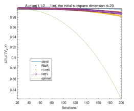
(a)

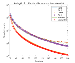
(b)

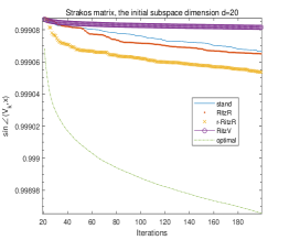
(c)

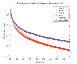
(d)

Fig. 1: The symmetric problems.

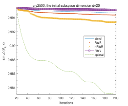
(a)

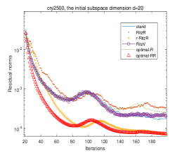
(b)

Fig. 2: The unsymmetric problem.

We now make several comments on the figures. Regarding $\sin\angle(\mathcal{V}_{k},x)$ for different kinds of subspaces $\mathcal{V}_{k},\ k=d+1,\ldots,m$, we clearly observe that the optimal subspace expansion approach “optimal” is always the best, the computable optimal subspace expansion approach “r-RitzR” is the second best, the computable optimal subspace approach “RitzR” is the third most effective, as is seen from Figure 1c and Figure 2a. They are all more effective than the Ritz subspace expansion approach “RitzV” and the standard subspace subspace approach “stand”. The latter two ones themselves win each other for the symmetric matrices, as indicated by Figure 1a and Figure 1c, but “RitzV” is not as good as “stand” for the unsymmetric matrix cry2500. More precisely, the computable optimal subspace expansion approach “RitzR” is better than “stand” and “RitzV” for the unsymmetric matrix and the symmetric Strakǒs matrix, but behaves very like “RitzV” for the symmetric matrix $A=\mathop{\operator@font diag}\nolimits(1,1/2,\ldots,1/10000)$. On the other hand, as the figures indicate, the three test problems are quite difficult as the desired $\lambda$ is clustered with some other eigenvalues for each problem, causing $\sin\angle(\mathcal{V}_{k},x)$ to decay very slowly for the five subspace expansion approaches including the optimal one. To summarize, the effectiveness of subspace expansion approaches is, in turn, “optimal”, “r-RitzR” and “RitzR”, and they are better than “RitzV” and “stand”; as for “RitzV” and “stand”, there is essentially no winner.

In contrast, the residual norms of the approximate eigenpairs exhibit more complicated features. Note that “stand”, “RitzR”, “RitzV”, and “optimal-R” all use the standard Rayleigh–Ritz method on respective subspaces $\mathcal{V}_{k+1},\ k=d,\ldots,m-1$, to compute the Ritz approximations of $(\lambda,x)$. As we have commented in the above and observed from the figures, $\sin\angle(\mathcal{V}_{k},x)$ decays slowly for all the subspace expansion approaches, and the residual norms of approximate eigenpairs obtained by “stand”, “RitzR”, “RitzV” and “optimal-R” decrease in a similar pattern.

However, the situation changes dramatically for “r-RitzR” and “optimal-RR”. First, “r-RitzR” computes considerably more accurate approximate eigenpairs than the afore-mentioned four methods at each iteration. Second, “r-RitzR” behaves very like “optimal-RR”, the ideally optimal one, meaning that the computable optimal “r-RitzR” almost computes best eigenpair approximations of $(\lambda,x)$ at each iteration. Third, “optimal-RR” outperforms “optimal-R” substantially, and converges much faster than the latter, though they work on the same subspace at each iteration. This indicates that the refined Rayleigh–Ritz method can outperform the standard Rayleigh–Ritz method on the same subspace considerably.

In summary, our experiments on the three test problems have demonstrated that “r-RitzR” is the best among the computable subspace expansion approaches, and the refined Rayleigh–Ritz method on the resulting generated subspaces behaves very like “optimal-RR”, i.e., the theoretical optimal subspace expansion approach.

5 Conclusions

We have considered the optimal subspace expansion problem for the general eigenvalue problem, and generalized the maximization characterization of $\cos\angle(\mathcal{V}_{w},x)$, one of Ye’s two main results, to the general case. Furthermore, we have found the solution $b_{w}$ to the maximization characterization problem of $\cos\angle(\mathcal{V}_{w},x)$. Based on the expression of $b_{w}$, we have analyzed the Ritz expansion approach, i.e., the RA method and argued that the Ritz vector may not be a good approximation to the optimal expansion vector $w_{opt}$.

Most importantly, we have established a few results on $w_{opt}$, $(I-P_{V})Aw_{opt}$, the theoretical optimal subspace $\mathcal{V}_{w_{opt}}$, and $\cos\angle(\mathcal{V}_{w_{opt}},x)$ for $A$ general and given their explicit expressions. We have analyzed the results in depth and obtained computable optimal replacements of $(I-P_{V})Aw_{opt}$ and $\mathcal{V}_{w_{opt}}$ within the framework of the standard, refined, harmonic and refined harmonic Rayleigh–Ritz methods. Taking the standard Rayleigh–Ritz method as an example, we have given implementation details on how to obtain the computable optimally expanded subspace $\mathcal{V}_{\widetilde{w}_{opt}}$ and made a cost comparison with the subspace expansion approach with some other expansion approaches such as the Lanczos or Arnoldi type expansion approach with $w=v_{k}$, the last column of $V_{k}$, the Ritz expansion approach, i.e., the RA method, with $w$ being the Ritz vector of $A$ from $\mathcal{V}_{k}$.

Our numerical experiments have demonstrated the advantages of the computable optimal expansion approaches over the afore-mentioned expansion approaches. Particularly, we have observed that the computable optimal subspace expansion approach using the refined Ritz vector of $A$ from ${\rm span}\{R_{k}\}$ behaves very like the theoretical optimal expansion approach since the eigenpair approximations obtained by the former are almost as accurate as those computed by the latter. This indicates that such computable optimal expansion approach is as good as the theoretical optimal one and is thus very promising when measuring the accuracy of approximate eigenpairs in terms of residual norms.

We have also proposed a potentially more robust subspace expansion approach that expanding $\mathcal{V}$ to $\mathcal{V}\oplus{\rm span}\{R\}$ and computing approximate eigenpairs with respect to $\mathcal{V}\oplus{\rm span}\{R\}$ in the next iteration. For the sake of length and focus, we do not further probe this approach in the current paper and leave it as future work.

It is well known that the harmonic Rayleigh–Ritz method is more suitable to compute interior eigenvalues and their associated eigenvectors than the standard Rayleigh–Ritz method [1, 19, 21]. Furthermore, since the standard and harmonic Rayleigh–Ritz methods may have convergence problems when computing eigenvectors [7, 10], we may gain much when using the refined Rayleigh–Ritz method [5, 10] and the refined harmonic Rayleigh–Ritz method [7, 9] correspondingly. As a matter of fact, for a sufficiently accurate subspace $\mathcal{V}$, the Ritz vector and the harmonic Ritz vector may be poor approximations to $x$ and can deviate from $x$ arbitrarily (cf. [19, pp. 284-5] and [7, Example 2]), but the refined Ritz vector and the refined harmonic Ritz vector are always excellent approximations to $x$ [19, pp. 291] and [7, Example 2], provided that the selected approximate eigenvalues converge to the desired eigenvalue $\lambda$ correctly. The advantages of the refined Rayleigh–Ritz method over the standard Rayleigh–Ritz method have also been justified by the numerical experiments in the last section. Therefore, it is preferable to expand the subspace using the refined Ritz vector and the refined harmonic Ritz vector from ${\rm span}\{R_{k}\}$ when exterior and interior eigenpairs of $A$ are required, respectively.

Based on the results in Section 3 and our numerical experiments, starting with a $k$-dimensional non-Krylov subspace with the residual $R_{k}$ defined by (5) and $\mathop{\operator@font rank}\nolimits(R_{k})\geq 2$, it is promising to develop four kinds of more practical restarted projection algorithms using computable optimal subspace expansion approaches.

As it is known, there are remarkable distinctions between the Arnoldi type expansion with $w=v_{k}$ and the RA method [11, 12], i.e., the Ritz expansion approach [24, 25], or the refined RA method, i.e., the refined Ritz expansion approach [24] as well as between SIRA or JD type methods and inexact SIA type methods: A large perturbation in $Aw$ of RA type methods or in $Bw$ of SIRA and JD type methods is allowed [8, 9, 22], while $Av_{k}$ in Arnoldi type methods or $Bv_{k}$ in SIA type methods must be computed with high accuracy until the approximate eigenpairs start to converge, and afterwards its solution accuracy can be relaxed in a manner inversely proportional to the residual norms of approximate eigenpairs [16, 17]. Keep these in mind. There will be a lot of important problems and issues that deserve considerations. For example, how large errors are allowed in $QQ^{H}x/\|QQ^{H}x\|$ when effectively expanding the subspace, where the columns of $Q$ form an orthonormal basis of ${\rm span}\{R_{k}\}$? This can be transformed into the problem of how large errors are allowed in the residual $R_{k}$. In practical computations, this problem becomes the one of how large errors are allowed in those computable optimal replacements of $QQ^{H}x/\|QQ^{H}x\|$ within the framework of the four kinds of projection methods, whenever perturbation errors exist in the computable optimal replacements of $QQ^{H}x/\|QQ^{H}x\|$. Is it possible to introduce the computable optimal expansion approaches into JD and SIRA type methods? All these need systematic exploration and analysis, and will constitute our future work.

References

- [1] Z. Bai, J. Demmel, J. Dongarra, A. Ruhe and H. Van der Vorst, Templates for the Solution of Algebraic Eigenvalue Problems: A Practical Guide, SIAM, Philadelphia, PA, 2000.
- [2] G. H. Golub and C. F. Van Loan, Matrix Computations, The Fourth Edition, The John Hopkins University, Baltimore, 2013.
- [3] M. Gu and S. C. Eisenstat, efficient algorithms for computing a strong rank-revealing QR factorization, SIAM J. Sci. Comput., 17 (1996), pp. 848–869.
- [4] Z. Jia, The convergence of generalized Lanczos methods for large unsymmetric eigenproblems, SIAM J. Matrix Anal. Appl., 16 (1995), pp. 843–862.
- [5] Z. Jia, Refined iterative algorithms based on Arnoldi’s process for unsymmmetric eigenproblems, Linear Algebra Appl., 259 (1997), pp. 1–23.
- [6] Z. Jia, Some theoretical comparisons of refined Ritz vectors and Ritz vectors, Science in China Ser. A Math., 47 (2004), Supp. 222–233.
- [7] Z. Jia, The convergence of harmonic Ritz values, harmonic Ritz vectors and refined harmonic Ritz vectors, Math. Comput., 74 (2005), pp. 1441–1456.
- [8] Z. Jia and C. Li, Inner iterations in the shift-invert residual Arnoldi method and the Jacobi–Davidson method, Sci. China Math., 57 (2014), pp. 1733–1752.
- [9] Z. Jia and C. Li, Harmonic and refined harmonic shift-invert residual Arnoldi and Jacobi–Davidson methods for interior eigenvalue problems, J. Comput. Appl. Math., 282 (2015), pp. 83–97.
- [10] Z. Jia and G. W. Stewart, An analysis of the Rayleigh–Ritz method for approximating eigenspaces, Math. Comput., 70 (2001), pp. 637–648.
- [11] C. Lee, Residual Arnoldi method: theory, package and experiments, Ph. D thesis, TR-4515, Department of Computer Science, University of Maryland at College Park, 2007.
- [12] C. Lee and G. W. Stewart, Analysis of the residual Arnoldi method, TR-4890, Department of Computer Science, University of Maryland at College Park, 2007.
- [13] G. Meurant, The Lanczos and Conjugate Gradient Algorithms: From Theory to Finite Precision Computations, SIAM, Philadelphia, PA, 2006.
- [14] B. N. Parlett, The Symmetric Eigenvalue Problem, SIAM, Philadelphia, PA, 1998.
- [15] Y. Saad, Numerical Methods for Large Eigenvalue Problems, Revised Version, SIAM, Philadephia, PA, 2011.
- [16] V. Simoncini, Variable accuracy of matrix-vector products in projection methods for eigencomputation, SIAM J. Numer. Anal., 43 (2005), pp. 1155–1174.
- [17] V. Simoncini and D. Szyld, Theory of inexact Krylov subspace methods and applications to scientific computing, SIAM J. Sci. Comput., 25(2003), pp. 454–477.
- [18] G. Sleijpen and H. van der Vorst, A Jacobi–Davidson iteration method for linear eigenvalue problems, SIAM J. Matrix Anal. Appl., 17 (1996), pp. 401–425. Reprinted in SIAM Review, (2000), pp. 267–293.
- [19] G. W. Stewart, Matrix Algorithms II: Eigensystems, SIAM, Philadelphia, PA, 2001.
- [20] G. W. Stewart and J.-G. Sun, Matrix Perturbation Theory, Academic Press Inc., Boston, 1990.
- [21] H. Van der Vorst, Computational Methods for Large Eigenvalue Problems, Elsevier, North Hollands, 2002.
- [22] H. Voss, A new justification of the Jacobi–Davidson method for large eigenproblems, Linear Algebra Appl., 424 (2007), pp. 448–455.
- [23] G. Wu, The convergence of harmonic Ritz vectors and harmonic Ritz values–revisited, SIAM. J. Matrix. Anal. Appl., 38 (2017), pp. 118–133.
- [24] G. Wu and L. Zhang, On expansion of search subspaces for large non-Hermitian eigenproblems, Linear Algebra Appl., 454 (2014), pp. 107–129.
- [25] Q. Ye, Optimal expansion of subspaces for eigenvector approximations, Linear Algebra Appl., 428 (2008), pp. 911–918.