Numerical methods for stochastic Volterra integral equations with weakly singular kernels^⋆

Abstract

In this paper, we first establish the existence, uniqueness and Hölder continuity of the solution to stochastic Volterra integral equations with weakly singular kernels. Then, we propose a $\theta$-Euler-Maruyama scheme and a Milstein scheme to solve the equations numerically and we obtain the strong rates of convergence for both schemes in $L^{p}$ norm for any $p\geq 1$. For the $\theta$-Euler-Maruyama scheme the rate is $\min\{1-\alpha,\frac{1}{2}-\beta\}~{}$ and for the Milstein scheme the rate is $\min\{1-\alpha,1-2\beta\}$ when $\alpha\neq\frac{1}{2}$, where $(0<\alpha<1,0<\beta<\frac{1}{2})$. These results on the rates of convergence are significantly different from that of the similar schemes for the stochastic Volterra integral equations with regular kernels. The difficulty to obtain our results is the lack of Itô formula for the equations. To get around of this difficulty we use instead the Taylor formula and then carry a sophisticated analysis on the equation the solution satisfies.

1 Introduction

Let $(\Omega,\mathscr{F},\mathbb{P})$ be a complete probability space with a filtration $\{\mathscr{F}_{t}\}_{0\leq t\leq 1}$ satisfying the usual condition. The expectation on this space is denoted by $\mathbb{E}$. Let $W(t):=(W_{1}(t),\cdots,W_{m}(t))^{T}$, $0\leq t\leq 1$, be an $m$-dimensional Wiener process defined on the probability space $(\Omega,\mathscr{F},\mathbb{P})$ adapted to the filtration $\mathscr{F}_{t}$. Assume $a:[0,1]\times\mathbb{R}^{d}\rightarrow\mathbb{R}^{d}$ and $b:[0,1]\times\mathbb{R}^{d}\rightarrow\mathbb{R}^{d\times m}$ satisfy some conditions that we shall specify in next section. In this paper we shall consider the numerical approximation of the following $d$-dimensional stochastic Volterra integral equations (SVIEs) with weakly singular kernel

$$X(t)=X_{0}+\int_{0}^{t}(t-s)^{-\alpha}a(X(s))ds+\int_{0}^{t}(t-s)^{-\beta}b(X(s))dW_{s},~{}~{}~{}t\in[0,1]\,,$$ (1.1)

where $\alpha\in(0,1)$, $\beta\in(0,\frac{1}{2})$ are two given positive numbers and the initial condition can be random and satisfies $\mathbb{E}|X_{0}|^{p}<\infty$ for any $p\geq 1$. We consider the interval $[0,1]$ for notational simplicity. It is easy to extend all the results of this paper to equation on any finite interval $[0,T]$ instead of $[0,1]$. When $\alpha=\beta=0$, the above stochastic differential equations (SDEs), including their numerical schemes, have been very well-studied. Many monographs can be found so that we are not going to give any references here. Relatively, the singular Volterra integral equations of the above form have been less studied. We mention some existence and uniqueness results under the (global) Lipschitz condition and the linear growth condition (see [1, 2, 3, 4]).

When $(t-s)^{-\alpha}$ and $(t-s)^{-\beta}$ are replaced by some nice functions, the numerical schemes of (regular) SVIEs have received attention only quite recently. Tudor [5] studied the strong convergence of one-step numerical approximations for Itô-Volterra equations, and he obtained the rate of convergence in the mean-square sense ($L_{p}$ when $p=2$ in our terminology here). Wen and Zhang [6] analysed an improved variant of the rectangular method for stochastic Volterra equation, and the order of convergence was shown to be $1.0$. Subsequently, Wang [7] approximated the solutions to SVIEs by means of solutions to a class of SDEs and he studied two numerical methods: stochastic theta method and splitting method. Xiao et al. [8] introduced a split-step collocation method for SVIEs, and the method was proved to be convergent with order $0.5$. Most relevant to our work is the work of Liang et al. [9] who found that Euler-Maruyama (EM) method can achieve a superconvergence of order $1.0$ if the kernel function in diffusion term satisfies certain boundary condition. More recently, for the Euler scheme for more general class of equations, such as SVIEs with delay, stochastic Volterra integro-differential equations and stochastic fractional integro-differential equations, we refer to [10, 11, 12, 13, 14].

To the best of our knowledge, there have been not yet numerical schemes for SVIEs with weakly singular kernel like the form in (1.1). The difficulty is probably the singularity of the integrand kernel: In this case the powerful and necessary tool of Itô formula commonly used previously does not exist for SVIEs with singular kernel. In this work we fill this gap by providing strong convergence rates of $\theta$-Euler-Maruyama scheme and Milstein scheme. Our results for the numerical parts are summarized as follows. For Euler scheme ($Y_{n}$ obtained from (2.3)) we shall prove that for any $p\geq 1$

$$\max_{n\in\{0,\cdots,N\}}\|X(t_{n})-Y_{n}\|_{L^{p}(\Omega;\mathbb{R}^{d})}\leq Ch^{\min\left(\frac{1}{2}-\beta,~{}1-\alpha\right)},$$

where $h$ is the mesh size. And for Milstein type scheme (the $Z_{n}$ given by (2.4)) we shall prove the estimate:

$$\max_{n\in\{0,\cdots,N\}}\|X(t_{n})-Z_{n}\|_{L^{p}(\Omega;\mathbb{R}^{d})}\leq\left\{\begin{array}[]{ll}Ch^{\min\{1-\alpha,1-2\beta\}},&\hbox{$\alpha\neq\frac{1}{2}$;}\\ C\max\{h^{\min\{\frac{1}{2},1-2\beta\}},h^{(1-\beta)}(\ln(\frac{1}{h}))^{1/2}\},&\hbox{$\alpha=\frac{1}{2}$.}\end{array}\right.$$

Since we can no longer use the Itô-Taylor formula for the sultion of the equation, we shall use only the Taylor formula combined with the techniques of classical fractional calculus, and discrete and continuous typed Gronwall inequalities with weakly singular kernels.

The remaining part of the paper is organized as follows. In Section $2$, some assumptions and preliminaries are introduced. The main results of the paper on the existence, uniqueness, and Hölder continuity of the solution and the strong convergence rate results are stated. When the kernel are singular it seems that the well-posedness of the equation has not been studied yet. Section $3$ studies the existence, uniqueness of the exact solution of the SVIEs with singular kernel. On the other hand, to obtain the rates of convergence of our schemes we also need to use th Hölder continuity of the solution. All of these are done in Section $3$. In Section $4$, we present a proof of the convergence results of $\theta$ Euler-Maruyama scheme. In Section $5$, we present a proof of the convergence results of Milstein-type scheme. In Section $6$, we present some numerical simulations to support our theoretical results.

2 Preliminaries and main results

We need to use the following generalized (discrete and continuous types) Gronwall inequalities with weakly singular kernels, whose proofs can be found in [15].

Lemma 2.1.

Let $b>0$ be a positive number. If the non-negative sequence $\{H_{n}\}$ satisfies the inequality

$$H_{n}\leq\pi_{n}+b\sum_{l=0}^{n-1}(n-l)^{-\gamma}H_{l},~{}~{}~{}0\leq n\leq N,$$

where the sequence $\{\pi_{n}\}$ is non-negative, and $0<\gamma<1$, then

$$H_{n}\leq E_{1-\gamma}(\Gamma(1-\gamma)n^{1-\gamma}b)\pi_{n},$$

where $\Gamma(a)=\int_{0}^{\infty}e^{-s}s^{a-1}ds$, $a>0$ is the Euler Gamma function, and

$$E_{a}(x):=\sum_{k=0}^{\infty}\frac{1}{\Gamma(ak+1)}x^{k}\,,\quad a>0$$

is the Mittag-Leffler function of $x\in\mathbb{R}$ (cf. [16]).

Lemma 2.2.

Let $I:=[0,1]$ and assume that
(i) $g\in C(I)$ (the set of real valued continuous functions on $I$) and $g$ is non-decreasing on $I$.
(ii) the continuous, non-negative function $H$ satisfies the inequality

$$H(t)\leq g(t)+b\int_{0}^{t}(t-s)^{-\gamma}H(s)ds$$

for constant $b>0$ and $0<\gamma<1$. Then

$$H(t)\leq E_{1-\gamma}(\Gamma(1-\gamma)t^{1-\gamma}b)g(t),~{}~{}~{}t\in I.$$

The assumptions that we are going to make about the coefficients in our main equation (1.1) are summarized as follows.

Assumption 1.

Assume that
(i) there exists positive constant $\hat{L}$ such that

$$|a(x)-a(y)|\vee|b(x)-b(y)|\leq\hat{L}|x-y|;$$

(ii) the function $a$ and $b$ satisfy the linear growth condition

$$|a(x)|\leq\hat{L}(1+|x|),~{}~{}|b(x)|\leq\hat{L}(1+|x|).$$

Assumption 2.

Assume that there exists positive constant $\hat{L}$ such that the derivatives of function $a$ satisfies

$$|\nabla a(x)-\nabla a(y)|\leq\hat{L}|x-y|;$$

We now show that Assumption 1 is sufficient to ensure the existence and uniqueness of the solution to equation (1.1).

Theorem 2.1.

Assume that the coefficients $a$ and $b$ satisfy Assumption 1. Then there is a unique solution $X(t)$ to (1.1), and the solution satisfies that for any $p\geq 1$,

$$\sup_{0\leq t\leq 1}\mathbb{E}|X(t)|^{p}\leq C_{p},$$ (2.1)

where and throughout the remaining part of the paper we denote by $C$ (or $C_{p}$) a generic constant (independent of $h$) which may have different values in different places.

We also need the Hölder continuity in the p-th ($p\geq 1$) moment of the exact solution.

Theorem 2.2.

Let the assumptions 1 and 2 are satisfied. Denote $\gamma(\alpha,\beta)=\min\{\frac{1}{2}-\beta,~{}1-\alpha\}$. Then for the solution $X$ to (1.1) we have for any $p\geq 1$,

$$\mathbb{E}|X(t)-X(r)|^{p}\leq C_{p}|t-r|^{p\gamma(\alpha,\beta)}\,,\quad\forall\ 0\leq r\leq t\leq 1\,.$$ (2.2)

The proofs of the above two theorems (Theorem 2.1 and 2.2) are given in Section 3.

Let $h>0$ be the mesh size. Throughout this paper, we consider only uniform mesh on $[0,1]$ by

$$t_{i}=ih,~{}~{}i=0,1,\cdots,N,~{}~{}h=\frac{1}{N}.$$

Denote $\eta(s)=t_{i}$ for $t_{i}\leq s<t_{i+1}$ and $\lfloor x\rfloor$ is the greatest integer less than or equal to $x$.

We first introduce the following $\theta$-Euler-Maruyama ($\theta$-EM ) and Milstein-type schemes for SVIEs with weakly singular kernel respectively as follows

$$\begin{split}Y_{n+1}=&Y_{0}+\theta\sum_{i=0}^{n}\int_{t_{i}}^{t_{i+1}}(t_{n+1}-s)^{-\alpha}a(Y_{i+1})ds+(1-\theta)\sum_{i=0}^{n}\int_{t_{i}}^{t_{i+1}}(t_{n+1}-s)^{-\alpha}a(Y_{i})ds\\ &+\sum_{i=0}^{n}\int_{t_{i}}^{t_{i+1}}(t_{n+1}-t_{i})^{-\beta}b(Y_{i})dW_{s},~{}~{}~{}n=0,1,\cdots,N-1,~{}~{}\theta\in[0,1],\end{split}$$ (2.3)

and

$$\begin{split}Z_{n+1}=&Z_{0}+\sum_{i=0}^{n}\int_{t_{i}}^{t_{i+1}}(t_{n+1}-s)^{-\alpha}a(Z_{i})ds+\sum_{i=0}^{n}\int_{t_{i}}^{t_{i+1}}(t_{n+1}-s)^{-\beta}b(Z_{i})dW_{s}\\ &+\sum_{i=0}^{n}\int_{t_{i}}^{t_{i+1}}(t_{n+1}-s)^{-\beta}b^{{}^{\prime}}(Z_{i})\bigg{(}\sum_{l=0}^{i-1}\int_{t_{l}}^{t_{l+1}}[(s-r)^{-\beta}-(t_{i}-r)^{-\beta}]b(Z_{l})dW_{r}\bigg{)}dW_{s}\\ &+\sum_{i=0}^{n}\int_{t_{i}}^{t_{i+1}}(t_{n+1}-s)^{-\beta}b^{{}^{\prime}}(Z_{i})\bigg{(}\int_{t_{i}}^{s}(s-r)^{-\beta}b(Z_{i})dW_{r}\bigg{)}dW_{s},~{}~{}~{}n=0,1,\cdots,N-1,\end{split}$$ (2.4)

where $Y_{0}=Z_{0}=X_{0}$.

The main results of this paper are the following strong rates of convergence of the $\theta$ Euler-Maruyama scheme (2.3) and Milstein-type scheme (2.4) for the solution of the SVIEs with weakly singular kernel (1.1). We shall provide their proofs in Sections 4 and 5, respectively.

Theorem 2.3.

If the functions $a$ and $b$ satisfy Assumption 1, then for any $p\geq 1$

$$\max_{n\in\{0,\cdots,N\}}\|X(t_{n})-Y_{n}\|_{L^{p}(\Omega;\mathbb{R}^{d})}\leq Ch^{\min\big{(}\frac{1}{2}-\beta,~{}1-\alpha\big{)}},$$

where $X$ is the exact solution of (1.1) and $Y_{n}$ is the numerical solution obtained from the $\theta$ Euler-Maruyama scheme dictated by (2.3).

Theorem 2.4.

If the functions $a$ and $b$ and their derivatives till the third order are bounded, and if the Assumption 1 and Assumption 2 are satisfied, then for any $p\geq 1$

$$\max_{n\in\{0,\cdots,N\}}\|X(t_{n})-Z_{n}\|_{L^{p}(\Omega;\mathbb{R}^{d})}\leq\left\{\begin{array}[]{ll}Ch^{\min\{1-\alpha,1-2\beta\}},&\hbox{$\alpha\neq\frac{1}{2}$;}\\ C\max\{h^{\min\{1/2,1-2\beta\}},h^{(1-\beta)}(\ln(\frac{1}{h}))^{1/2}\},&\hbox{$\alpha=\frac{1}{2}$.}\end{array}\right.$$

Remark 2.1.

When the singular parameter $\alpha=\beta=0$, the above two theorems say that the $\theta$ Euler-Maruyama scheme (2.3) and Milstein-type scheme (2.4) recover the optimal convergence rate of order $0.5$ and $1$, respectively.

3 The existence, uniqueness and Hölder continuity of the exact solution

In this section we provide proofs for Theorems 2.1 and 2.2.

Proof of Theorem 2.1.

We assume $p\geq 2$. The case $1\leq p<2$ can be derived from Lyapunov inequality (namely $\|F\|_{p}\leq\|F\|_{q}$ for $1\leq p\leq q\leq\infty$). We borrow some ideas from [1, Theorem 1], where the authors studied the existence and uniqueness of the equations

$$X(t)=X_{0}+\frac{1}{\Gamma(\alpha)}\bigg{(}\int_{0}^{t}(t-s)^{\alpha-1}b(X(s))ds+\int_{0}^{t}(t-s)^{\alpha-1}\sigma(X(s))dW_{s}\bigg{)},\quad\alpha>\frac{1}{2}$$

in the space $L^{2}$. Here, we consider SVIEs with two different singular kernel, which allow the singular parameter $\alpha$ in the drift term vary from $0$ to $1$ and we consider the solution in $L^{p}$ for any $p\in[1,\infty)$. Moreover, we shall prove that $\mathbf{T}:\mathbb{S}^{p}(0,1)\rightarrow\mathbb{S}^{p}(0,1)$ is a contraction mapping with respect to more general norm ($L^{p}$ norm, $p\geq 1$). Thus, some new techniques will be needed. Denote by $\mathbb{S}^{p}(0,1)$ the Banach space of the stochastic process that are measurable, $\mathscr{F}_{t}$-adapted, where the norm of the process is defined by

$$\|X\|_{\mathbb{S}^{p}}:=\sup\limits_{0\leq t\leq 1}\left(\mathbb{E}|X(t)|^{p}\right)^{1/p}<\infty.$$

Define operators $\mathbf{T}:\mathbb{S}^{p}(0,1)\rightarrow\mathbb{S}^{p}(0,1)$ by

$$\mathbf{T}\lambda(t):=X_{0}+\int_{0}^{t}(t-s)^{-\alpha}a(\lambda(s))ds+\int_{0}^{t}(t-s)^{-\beta}b(\lambda(s))dW_{s}.$$

Obviously, the operators $\mathbf{T}$ are well defined. Let $\kappa$ be a positive constant such that

$$\kappa>2^{p-1}\hat{L}^{p}\left(\frac{T^{(1-\alpha)p}}{1-\alpha}+\frac{T^{(1-2\beta)p}}{1-2\beta}\right)\Gamma(1-\max(\alpha,2\beta)),$$ (3.1)

where $\Gamma(\cdot)$ is the Gamma function. We introduce a new weighted norm $\|\cdot\|_{\kappa}$ by

$$\|X\|_{\kappa}:=\sup_{t\in[0,1]}\sqrt{\frac{\mathbb{E}(|X(t)|^{p})}{E_{1-\max(\alpha,2\beta)}(\kappa t^{1-\max(\alpha,2\beta)})}},$$

where $E_{1-\max(\alpha,2\beta)}(\cdot)$ is the Mittag-Leffler function. It is easy to verify that $\|\cdot\|_{\mathbb{S}^{p}}$ and $\|\cdot\|_{\kappa}$ are equivalent. Next, we show that $\mathbf{T}$ is contractive with respect to the norm $\|\cdot\|_{\kappa}$. In fact, for any $\lambda,\mu\in\mathbb{S}^{2}(0,1)$, we have by Jensen’s inequality

$$\mathbb{E}|\mathbf{T}\lambda(t)-\mathbf{T}\mu(t)|^{p} \leq 2^{p-1}\mathbb{E}\left|\int_{0}^{t}(t-s)^{-\alpha}(a(\lambda(s))-a(\mu(s)))ds\right|^{p}$$ (3.2)

$$+2^{p-1}\mathbb{E}\left|\int_{0}^{t}(t-s)^{-\beta}(b(\lambda(s))-b(\mu(s)))dW_{s}\right|^{p}$$

$$\leq 2^{p-1}\left(\int_{0}^{t}(t-s)^{-\alpha}ds\right)^{p-1}\cdot\hat{L}^{p}\int_{0}^{t}(t-s)^{-\alpha}\mathbb{E}|\lambda(s)-\mu(s)|^{p}ds$$

$$+2^{p-1}\hat{L}^{p}\left(\int_{0}^{t}(t-s)^{-2\beta}ds\right)^{p/2-1}\mathbb{E}\int_{0}^{t}(t-s)^{-2\beta}|\lambda(s)-\mu(s)|^{p}ds$$

$$\leq 2^{p-1}\hat{L}^{p}\left(\frac{T^{(1-\alpha)p}}{1-\alpha}+\frac{T^{(1-2\beta)p}}{1-2\beta}\right)\int_{0}^{t}(t-s)^{-\max(\alpha,2\beta)}\mathbb{E}|\lambda(s)-\mu(s)|^{p}ds.$$

Hence, by Lemma 2.2 we have

$$\frac{\mathbb{E}|\mathbf{T}\lambda(t)-\mathbf{T}\mu(t)|^{p}}{E_{1-\max(\alpha,2\beta)}(\kappa t^{1-\max(\alpha,2\beta)})}$$

$$\leq 2^{p-1}\hat{L}^{p}\left(\frac{T^{(1-\alpha)p}}{1-\alpha}+\frac{T^{(1-2\beta)p}}{1-2\beta}\right)\frac{\int_{0}^{t}(t-s)^{-\max(\alpha,2\beta)}E_{1-\max(\alpha,2\beta)}(\kappa s^{1-\max(\alpha,2\beta)})ds}{E_{1-\max(\alpha,2\beta)}(\kappa t^{1-\max(\alpha,2\beta)})}\|\lambda-\mu\|_{\kappa}^{p}$$

$$\leq 2^{p-1}\hat{L}^{p}\left(\frac{T^{(1-\alpha)p}}{1-\alpha}+\frac{T^{(1-2\beta)p}}{1-2\beta}\right)\frac{\Gamma(1-\max(\alpha,2\beta))}{\kappa}\|\lambda-\mu\|_{\kappa}^{p}$$

$$=\rho\|\lambda-\mu\|_{\kappa}^{p},$$

where

$$\rho=2^{p-1}\hat{L}^{p}\left(\frac{T^{(1-\alpha)p}}{1-\alpha}+\frac{T^{(1-2\beta)p}}{1-2\beta}\right)\frac{\Gamma(1-\max(\alpha,2\beta))}{\kappa}$$

and where we used

$$\int_{0}^{t}(t-s)^{-\max(\alpha,2\beta)}E_{1-\max(\alpha,2\beta)}(\kappa s^{1-\max(\alpha,2\beta)})ds\leq\frac{\Gamma(1-\max(\alpha,2\beta))}{\kappa}E_{1-\max(\alpha,2\beta)}(\kappa t^{1-\max(\alpha,2\beta)})\,.$$

By our choice of $\kappa$ (namely (3.1)) we see that that $\rho<1$. Thus we conclude that $\mathbf{T}:\mathbb{S}^{p}(0,1)\rightarrow\mathbb{S}^{p}(0,1)$ is a contraction mapping. By Banach contractive mapping theorem, we see that there exists a unique solution in $\mathbb{S}^{p}(0,1)$.

The bound (2.1) follows easily from the above argument (e.g. (3.2) with $\mu=0$) and the linear growth condition of the functions $a$ and $b$. ∎

Proof of Theorem 2.2.

We continue to assume $p\geq 2$. The case $1\leq p<2$ can be proved by using a Lyapunov inequality.  Let $X(t)$ satisfy (1.1). We can write

$$X(t)-X(r)= \bigg{(}\int_{0}^{t}(t-s)^{-\alpha}a(X(s))ds-\int_{0}^{r}(r-s)^{-\alpha}a(X(s))ds\bigg{)}$$

$$+\bigg{(}\int_{0}^{t}(t-s)^{-\beta}b(X(s))dW_{s}-\int_{0}^{r}(r-s)^{-\beta}b(X(s))dW_{s}\bigg{)}$$

$$=:I_{41}+I_{42}.$$

Obviously, $I_{42}$ can be written as

$$I_{42}=\int_{0}^{r}[(t-s)^{-\beta}-(r-s)^{-\beta}]b(X(s))dW_{s}+\int_{r}^{t}(t-s)^{-\beta}b(X(s))dW_{s}=:I_{421}+I_{422}\,.$$

Then by Burkholder-Davis-Gundy inequality, we have

$$\mathbb{E}|I_{421}|^{p}= \mathbb{E}\left|\int_{0}^{r}[(t-s)^{-\beta}-(r-s)^{-\beta}]b(X(s))dW_{s}\right|^{p}$$

$$\leq C_{p}\mathbb{E}\left(\int_{0}^{r}\left|[(t-s)^{-\beta}-(r-s)^{-\beta}]b(X(s))\right|^{2}ds\right)^{p/2}\,.$$

Denote

$$\rho_{t,r}:=\int_{0}^{r}[(t-s)^{-\beta}-(r-s)^{-\beta}]^{2}ds\,.$$

Since $\phi(x)=x^{p/2}$, $x>0$ is convex, applying Jensen’s inequality we have

$$\left(\frac{1}{\rho_{t,r}}\int_{0}^{r}\left|[(t-s)^{-\beta}-(r-s)^{-\beta}]b(X(s))\right|^{2}ds\right)^{p/2}$$

$$\qquad\leq\frac{1}{\rho_{t,r}}\int_{0}^{r}\left|(t-s)^{-\beta}-(r-s)^{-\beta}\right|^{2}\left|b(X(s))\right|^{p}ds\,.$$ (3.3)

Thus we have

$$\mathbb{E}|I_{421}|^{p}\leq C_{p}\rho_{t,r}^{\frac{p}{2}-1}\int_{0}^{r}\left|(t-s)^{-\beta}-(r-s)^{-\beta}\right|^{2}\mathbb{E}\left|b(X(s))\right|^{p}ds$$

$$\leq C_{p}\rho_{t,r}^{\frac{p}{2}-1}\int_{0}^{r}\left|(t-s)^{-\beta}-(r-s)^{-\beta}\right|^{2}\mathbb{E}(1+\left|X(s)\right|)^{p}ds$$

$$\leq C_{p}\rho_{t,r}^{\frac{p}{2}-1}\int_{0}^{r}\left|(t-s)^{-\beta}-(r-s)^{-\beta}\right|^{2}ds=\rho_{t,r}^{\frac{p}{2}}\,.$$ (3.4)

Now we need to obtain a sharp bound on $\rho_{t,r}$

$$\rho_{t,r}= \int_{0}^{r}[(t-s)^{-\beta}-(r-s)^{-\beta}]^{2}ds$$

$$= \beta^{2}\int_{0}^{r}\left(\int_{r}^{t}(\tau-s)^{-\beta-1}d\tau\right)^{2}ds$$

$$= \beta^{2}\int_{0}^{r}\int_{r}^{t}\int_{r}^{t}(\tau_{1}-s)^{-\beta-1}(\tau_{2}-s)^{-\beta-1}d\tau_{1}d\tau_{2}ds$$

$$= 2\beta^{2}\int_{r<\tau_{1}<\tau_{2}\leq t}\int_{0}^{r}(\tau_{1}-s)^{-\beta-1}(\tau_{2}-s)^{-\beta-1}dsd\tau_{1}d\tau_{2}$$

$$\leq 2\beta^{2}\int_{r<\tau_{1}<\tau_{2}\leq t}\int_{0}^{r}(\tau_{1}-s)^{-\beta-1}(\tau_{2}-r)^{-\beta-1}dsd\tau_{1}d\tau_{2}$$

$$= 2\beta\int_{r<\tau_{1}<\tau_{2}\leq t}\left[(\tau_{1}-r)^{-\beta}-\tau_{1}^{-\beta}\right](\tau_{2}-r)^{-\beta-1}d\tau_{1}d\tau_{2}$$

$$\leq 2\beta\int_{r<\tau_{1}<\tau_{2}\leq t}(\tau_{1}-r)^{-\beta}(\tau_{2}-r)^{-\beta-1}d\tau_{1}d\tau_{2}$$

$$= \frac{2\beta}{1-\beta}\int_{r}^{t}(\tau_{2}-r)^{-2\beta}d\tau_{2}$$

$$= \frac{2\beta}{(1-\beta)(1-2\beta)}(t-r)^{1-2\beta}\,.$$

This together with (3.4) implies

$$\mathbb{E}|I_{421}|^{p}\leq C_{p}(t-r)^{p(\frac{1}{2}-\beta)}\,.$$ (3.5)

Analogously to (3.4), if we denote

$$\tilde{\rho}_{t,r}=\int_{r}^{t}(t-s)^{-2\beta}ds=\frac{(t-r)^{1-2\beta}}{1-2\beta}\,.$$

Then we have

$$\mathbb{E}|I_{422}|^{p}\leq C_{p}\tilde{\rho}_{t,r}^{p/2}\leq C_{p}(t-r)^{p(\frac{1}{2}-\beta)}\,.$$ (3.6)

Combining this with (3.5) we have

$$\mathbb{E}|I_{42}|^{p}\leq C_{p}(t-r)^{p(\frac{1}{2}-\beta)}\,.$$ (3.7)

For the term $I_{41}$

$$\mathbb{E}|I_{41}|^{p}\leq 2^{p}\mathbb{E}\left|\int_{0}^{r}[(t-s)^{-\alpha}-(r-s)^{-\alpha}]a(X(s))ds\right|^{p}$$

$$\qquad+2^{p}\mathbb{E}\left|\int_{r}^{t}(t-s)^{-\alpha}a(X(s))ds\right|^{p}=:I_{411}+I_{412}\,.$$

In the same way as for (3.5) we have

$$I_{411}\leq \left(\int_{0}^{r}\left|(t-s)^{-\alpha}-(r-s)^{-\alpha}\right|ds\right)^{p}$$

$$\leq C_{p}\left(\int_{0}^{r}\int_{r}^{t}(\tau-s)^{-{\alpha}-1}d\tau ds\right)^{p}$$

$$= C_{p}\left(\int_{r}^{t}\int_{0}^{r}(\tau-s)^{-{\alpha}-1}dsd\tau\right)^{p}$$

$$\leq C_{p}\left(\int_{r}^{t}(\tau-r)^{-{\alpha}}d\tau\right)^{p}=C_{p}(t-r)^{(1-\alpha)p}\,.$$

In the similar way, we can prove that

$$\mathbb{E}|I_{412}|^{2}\leq C_{p}(t-r)^{p(1-\alpha)}.$$

This completes the proof of the theorem. ∎

4 Convergence rate of $\theta$-Euler-Maruyama scheme

In this section we provide proof of the $\theta$ Euler-Maruyama scheme, namely, Theorem 2.3. We denote the local truncation errors of the $\theta$ Euler-Maruyama scheme by

$$\begin{split}R_{h}^{E}(t_{n+1})=&\theta\sum_{i=0}^{n}\int_{t_{i}}^{t_{i+1}}(t_{n+1}-s)^{-\alpha}(a(X(s))-a(X(t_{i+1})))ds\\ &+(1-\theta)\sum_{i=0}^{n}\int_{t_{i}}^{t_{i+1}}(t_{n+1}-s)^{-\alpha}(a(X(s))-a(X(t_{i})))ds\\ &+\sum_{i=0}^{n}\int_{t_{i}}^{t_{i+1}}(t_{n+1}-s)^{-\beta}b(X(s))-(t_{n+1}-t_{i})^{-\beta}b(X(t_{i}))dW_{s}\\ =&:I_{1}+I_{2}+I_{3}\,.\end{split}$$ (4.1)

Lemma 4.1.

If Assumption 1 holds, then for the local truncation error $R_{h}^{E}(t_{n+1})$, there is a constant $C$ such that for any $p\geq 1$

$$\mathbb{E}|R_{h}^{E}(t_{n+1})|^{p}\leq Ch^{\gamma(\alpha,\beta)p},$$

where $\gamma(\alpha,\beta)=\min\{\frac{1}{2}-\beta,~{}1-\alpha\}$.

Proof.

By (4.1)

$$\begin{split}\mathbb{E}|I_{3}|^{p}\leq&\mathbb{E}\left|\int_{0}^{t_{n+1}}[(t_{n+1}-s)^{-\beta}-(t_{n+1}-\eta(s))^{-\beta}]b(X(s))dW_{s}\right|^{p}\\ &+\mathbb{E}\left|\int_{0}^{t_{n+1}}(t_{n+1}-\eta(s))^{-\beta}[b(X(s))-b(X({\eta(s)}))]dW_{s}\right|^{p}=:I_{31}+I_{32}.\end{split}$$ (4.2)

Furthermore, using Assumption 1 and Theorem 2.1, we have

$$I_{31}\leq \mathbb{E}\bigg{(}\int_{0}^{t_{n+1}}[(t_{n+1}-s)^{-\beta}-(t_{n+1}-\eta(s))^{-\beta}]^{2}|b(X(s))|^{2}ds\bigg{)}^{\frac{p}{2}}.$$

Let

$$\rho_{n+1}=\int_{0}^{t_{n+1}}[(t_{n+1}-s)^{-\beta}-(t_{n+1}-\eta(s))^{-\beta}]^{2}ds\,.$$

Since $\phi(x)=x^{p/2}\,,x>0$ is convex by Jensen’s inequality, we have

$$\left(\frac{1}{\rho_{n+1}}\int_{0}^{t_{n+1}}[(t_{n+1}-s)^{-\beta}-(t_{n+1}-\eta(s))^{-\beta}]^{2}|b(X(s))|^{2}ds\right)^{\frac{p}{2}}$$

$$\leq\frac{1}{\rho_{n+1}}\int_{0}^{t_{n+1}}[(t_{n+1}-s)^{-\beta}-(t_{n+1}-\eta(s))^{-\beta}]^{2}|b(X(s))|^{p}ds.$$

Hence,

$$I_{31}\leq C\rho_{n+1}^{\frac{p}{2}-1}\int_{0}^{t_{n+1}}[(t_{n+1}-s)^{-\beta}-(t_{n+1}-\eta(s))^{-\beta}]^{2}\mathbb{E}(1+|X(s)|)^{p}ds\leq C\rho_{n+1}^{\frac{p}{2}}.$$ (4.3)

Now, we give a sharp estimate for $\rho_{n+1}$

$$\rho_{n+1}= C\int_{0}^{t_{n+1}}[(t_{n+1}-s)^{-\beta}-(t_{n+1}-\eta(s))^{-\beta}]^{2}ds$$

$$= C\sum_{i=0}^{n}\int_{t_{i}}^{t_{i+1}}\left|\beta\int_{t_{i}}^{s}(t_{n+1}-\tau)^{-\beta-1}d\tau\right|^{2}ds$$

$$\leq C\beta^{2}\sum_{i=0}^{n}\int_{t_{i}}^{t_{i+1}}\left|\int_{t_{i}}^{t_{i+1}}(t_{n+1}-t_{i+1})^{-\beta-1}d\tau\right|^{2}ds$$ (4.4)

$$\leq C\beta^{2}h^{1-2\beta}\sum_{i=0}^{n}(n-i)^{-2(\beta+1)}\leq Ch^{1-2\beta}.$$

Combining this with (4.3), we have

$$I_{31}\leq Ch^{(1-2\beta)\frac{p}{2}}.$$

Let $\widetilde{\rho}_{n+1}=\int_{0}^{t_{n+1}}(t_{n+1}-\eta(s))^{-2\beta}ds$. By an analysis similar to the above, we have

$$I_{32}\leq C_{p}\widetilde{\rho}_{n+1}^{\frac{p}{2}-1}\int_{0}^{t_{n+1}}(t_{n+1}-\eta(s))^{2}\mathbb{E}|X(s)-X(\eta(s))|^{p}ds,$$

where Assumption 1 was used. Using Theorem 2.2, one sees that

$$I_{32}\leq Ch^{\gamma(\alpha,\beta)p}.$$

Thus,

$$\mathbb{E}|I_{3}|^{2}\leq Ch^{\gamma(\alpha,\beta)p}.$$

In a similar manner, by Hölder inequality and Jensen’s inequality, one also has

$$\mathbb{E}|I_{1}|^{2}\leq Ch^{p(1-\alpha)},~{}~{}~{}\mathbb{E}|I_{2}|^{2}\leq Ch^{p(1-\alpha)}.$$

Summarizing the above arguments the desired assertion follows. ∎

Proof of Theorem 2.3.

Denote $\varepsilon_{n+1}:=X(t_{n+1})-Y_{n+1}$. It follows from (1.1), (2.3) and (4.1)

$$\begin{split}\varepsilon_{n+1}=&R_{h}^{E}(t_{n+1})+\theta\sum_{i=0}^{n}\int_{t_{i}}^{t_{i+1}}(t_{n+1}-s)^{-\alpha}(a(X_{t_{i+1}})-a(Y_{i+1}))ds\\ &+(1-\theta)\sum_{i=0}^{n}\int_{t_{i}}^{t_{i+1}}(t_{n+1}-s)^{-\alpha}(a(X_{t_{i}})-a(Y_{i}))ds\\ &+\sum_{i=0}^{n}\int_{t_{i}}^{t_{i+1}}(t_{n+1}-s)^{-\beta}(b(X_{t_{i}})-b(Y_{i}))dW_{s}.\end{split}$$ (4.5)

Let

$$\varepsilon_{\hat{s}}=\sum_{i=0}^{N-1}\varepsilon_{i+1}~{}\chi_{s\in[t_{i},t_{i+1}]},~{}~{}~{}\varepsilon_{\check{s}}=\sum_{i=0}^{N-1}\varepsilon_{i}~{}\chi_{s\in[t_{i},t_{i+1}]},$$

where

$$\chi_{s\in[t_{i},t_{i+1}]}=\left\{\begin{array}[]{ll}1,&\hbox{$s\in[t_{i},t_{i+1}]$;}\\ 0,&\hbox{\text{otherwise}.}\end{array}\right.$$

Then

$$\mathbb{E}|\varepsilon_{n+1}|^{p} \leq 4^{p-1}\mathbb{E}|R_{h}^{E}(t_{n+1})|^{p}+4^{p-1}\theta^{p}\mathbb{E}\big{|}\int_{0}^{t_{n+1}}(t_{n+1}-s)^{-\alpha}(a(X_{t_{i+1}})-a(Y_{i+1}))ds\big{|}^{p}$$ (4.6)

$$+4^{p-1}(1-\theta)^{p}\mathbb{E}\big{|}\int_{0}^{t_{n+1}}(t_{n+1}-s)^{-\alpha}(a(X_{t_{i}})-a(Y_{i}))ds\big{|}^{p}$$

$$+4^{p-1}\mathbb{E}\big{|}\int_{0}^{t_{n+1}}(t_{n+1}-\eta(s))^{-\beta}(b(X_{t_{i}})-b(Y_{i}))dW_{s}\big{|}^{p}$$

$$\leq C\bigg{\{}\mathbb{E}|R_{h}^{E}(t_{n+1})|^{p}+\bigg{(}\int_{0}^{t_{n+1}}(t_{n+1}-s)^{-\alpha}ds\bigg{)}^{p-1}\int_{0}^{t_{n+1}}(t_{n+1}-s)^{-\alpha}\mathbb{E}|\varepsilon_{\hat{s}}|^{p}ds$$

$$+\bigg{(}\int_{0}^{t_{n+1}}(t_{n+1}-s)^{-\alpha}ds\bigg{)}^{p-1}\int_{0}^{t_{n+1}}(t_{n+1}-s)^{-\alpha}\mathbb{E}|\varepsilon_{\check{s}}|^{p}ds$$

$$+\left(\int_{0}^{t_{n+1}}(t_{n+1}-\eta(s))^{-2\beta}ds\right)^{\frac{p}{2}-1}\int_{0}^{t_{n+1}}(t_{n+1}-s)^{-2\beta}\mathbb{E}|\varepsilon_{\check{s}}|^{p}ds\bigg{\}},$$

where Assumption 1 and Jensen’s inequality were used. Then,

$$\int_{t_{i}}^{t_{i+1}}(t_{n+1}-s)^{-\alpha}ds=\frac{(t_{n+1}-t_{i})^{1-\alpha}-(t_{n+1}-t_{i+1})^{1-\alpha}}{1-\alpha}=\frac{h^{1-\alpha}[(n+1-i)^{1-\alpha}-(n-i)^{1-\alpha}]}{1-\alpha}.$$ (4.7)

Note that

$$(n+1-i)^{1-\alpha}-(n-i)^{1-\alpha}$$

$$=(n+1-i)^{1-\alpha}[1-(1-\frac{1}{n+1-i})^{1-\alpha}]$$

$$=(n+1-i)^{-\alpha}\big{[}1-\theta_{n,i}\frac{1}{n+1-i}\big{]}^{-\alpha}.$$

Since $1-\theta_{n,i}\frac{1}{n+1-i}\geq\frac{1}{2}$, we have

$$(n+1-i)^{1-\alpha}-(n-i)^{1-\alpha}\leq 2^{\alpha}(n+1-i)^{-\alpha}.$$ (4.8)

Combining the above results with (4.6),we obtain

$$\begin{split}\mathbb{E}|\varepsilon_{n+1}|^{p}\leq&C\bigg{[}\mathbb{E}|R_{h}^{E}(t_{n+1})|^{p}+h^{1-\alpha}\sum_{i=0}^{n}\mathbb{E}|\varepsilon_{i+1}|^{p}\\ &+h^{1-\max(\alpha,2\beta)}\sum_{i=0}^{n}\mathbb{E}|\varepsilon_{i}|^{p}+h^{1-\max(\alpha,2\beta)}\sum_{i=0}^{n}(n+1-i)^{-\max(\alpha,2\beta)}\mathbb{E}|\varepsilon_{i}|^{p}\bigg{]}.\end{split}$$ (4.9)

The final result follows from Lemma 4.1 and Lemma 2.1. ∎

5 Convergence rate of Milstein-type scheme

In this section we provide a proof for the strong convergence rate of Milstein scheme, i.e. Theorem 2.4. We denote

$$\begin{split}R_{h}^{M}(t_{n+1})=&X(t_{n+1})-X_{0}-\sum_{i=0}^{n}\int_{t_{i}}^{t_{i+1}}(t_{n+1}-s)^{-\alpha}a(X(t_{i}))ds-\sum_{i=0}^{n}\int_{t_{i}}^{t_{i+1}}(t_{n+1}-s)^{-\beta}b(X(t_{i}))dW_{s}\\ &-\sum_{i=0}^{n}\int_{t_{i}}^{t_{i+1}}(t_{n+1}-s)^{-\beta}b^{{}^{\prime}}(X(t_{i}))\bigg{(}\int_{0}^{t_{i}}[(s-r)^{-\beta}-(t_{i}-r)^{-\beta}]b(X(r))dW_{r}\bigg{)}dW_{s}\\ &-\sum_{i=0}^{n}\int_{t_{i}}^{t_{i+1}}(t_{n+1}-s)^{-\beta}b^{{}^{\prime}}(X(t_{i}))\bigg{(}\int_{t_{i}}^{s}(s-r)^{-\beta}b(X(r))dW_{r}\bigg{)}dW_{s}\,.\end{split}$$ (5.1)

From (1.1), we have

$$X({t_{n+1}})=X_{0}+\sum_{i=0}^{n}\int_{t_{i}}^{t_{i+1}}(t_{n+1}-s)^{-\alpha}a(X(s))ds+\sum_{i=0}^{n}\int_{t_{i}}^{t_{i+1}}(t_{n+1}-s)^{-\beta}b(X(s))dW_{s}.$$ (5.2)

Using the Taylor expansions of function $a(X(s))$ and $b(X(s))$ at $X(t_{i})$, we get

$$a(X(s))= a(X(t_{i}))+a^{{}^{\prime}}(X(t_{i}))(X(s)-X(t_{i}))$$

$$+\frac{a^{{}^{\prime\prime}}(X(t_{i}))}{2!}(X(s)-X(t_{i}))^{2}+\frac{a^{{}^{\prime\prime\prime}}(X_{t_{i,\theta_{1}}})}{3!}(X(s)-X(t_{i}))^{3},$$ (5.3)

and

$$b(X(s))= b(X(t_{i}))+b^{{}^{\prime}}(X(t_{i}))(X(s)-X(t_{i}))$$

$$+\frac{b^{{}^{\prime\prime}}(X(t_{i}))}{2!}(X(s)-X(t_{i}))^{2}+\frac{b^{{}^{\prime\prime\prime}}(X_{t_{i,\theta_{2}}})}{3!}(X(s)-X(t_{i}))^{3},$$ (5.4)

where $X_{t_{i,\theta_{1}}}$, $X_{t_{i,\theta_{2}}}$ are between $X({t_{i}})$ and $X(s)$. Substituting (5) and (5) to (5.2), one finds

$$X({t_{n+1}})= X_{0}+\sum_{i=0}^{n}\int_{t_{i}}^{t_{i+1}}(t_{n+1}-s)^{-\alpha}a(X(t_{i}))ds+\sum_{i=0}^{n}\int_{t_{i}}^{t_{i+1}}(t_{n+1}-s)^{-\beta}b(X(t_{i}))dW_{s}$$

$$+\sum_{i=0}^{n}\int_{t_{i}}^{t_{i+1}}(t_{n+1}-s)^{-\alpha}a^{{}^{\prime}}(X(t_{i}))(X(s)-X(t_{i}))ds$$

$$+\sum_{i=0}^{n}\int_{t_{i}}^{t_{i+1}}(t_{n+1}-s)^{-\beta}b^{{}^{\prime}}(X(t_{i}))(X(s)-X(t_{i}))dW_{s}$$

$$+\frac{1}{2!}\sum_{i=0}^{n}\int_{t_{i}}^{t_{i+1}}(t_{n+1}-s)^{-\alpha}a^{{}^{\prime\prime}}(X(t_{i}))(X(s)-X(t_{i}))^{2}ds$$ (5.5)

$$+\frac{1}{2!}\sum_{i=0}^{n}\int_{t_{i}}^{t_{i+1}}(t_{n+1}-s)^{-\beta}b^{{}^{\prime\prime}}(X(t_{i}))(X(s)-X(t_{i}))^{2}dW_{s}$$

$$+\frac{1}{3!}\sum_{i=0}^{n}\int_{t_{i}}^{t_{i+1}}(t_{n+1}-s)^{-\alpha}a^{{}^{\prime\prime\prime}}(X_{t_{i,\theta_{1}}})(X(s)-X(t_{i}))^{3}ds$$

$$+\frac{1}{3!}\sum_{i=0}^{n}\int_{t_{i}}^{t_{i+1}}(t_{n+1}-s)^{-\beta}b^{{}^{\prime\prime\prime}}(X_{t_{i,\theta_{2}}})(X(s)-X(t_{i}))^{3}dW_{s}.$$

It follows from (1.1) that,

$$\begin{split}X(s)-X(t_{i})=&\int_{0}^{t_{i}}[(s-r)^{-\alpha}-(t_{i}-r)^{-\alpha}]a(X(r))dr+\int_{t_{i}}^{s}(s-r)^{-\alpha}a(X(r))dr\\ &+\int_{0}^{t_{i}}[(s-r)^{-\beta}-(t_{i}-r)^{-\beta}]b(X(r))dW_{r}+\int_{t_{i}}^{s}(s-r)^{-\beta}b(X(r))dW_{r}.\end{split}$$ (5.6)

Substituting (5.6) into (5), one arrives at

$$\begin{split}X({t_{n+1}})=&X_{0}+\sum_{i=0}^{n}\int_{t_{i}}^{t_{i+1}}(t_{n+1}-s)^{-\alpha}a(X(t_{i}))ds+\sum_{i=0}^{n}\int_{t_{i}}^{t_{i+1}}(t_{n+1}-s)^{-\beta}b(X(t_{i}))dW_{s}\\ &+\sum_{i=0}^{n}\int_{t_{i}}^{t_{i+1}}(t_{n+1}-s)^{-\beta}b^{{}^{\prime}}(X(t_{i}))\int_{0}^{t_{i}}[(s-r)^{-\beta}-(t_{i}-r)^{-\beta}]b(X(r))dW_{r}dW_{s}\\ &+\sum_{i=0}^{n}\int_{t_{i}}^{t_{i+1}}(t_{n+1}-s)^{-\beta}b^{{}^{\prime}}(X(t_{i}))\int_{t_{i}}^{s}(s-r)^{-\beta}b(X(r))dW_{r}dW_{s}\\ &+\tilde{\beta}+\tilde{\gamma}+\tilde{\delta}+R_{n},\end{split}$$ (5.7)

where

$$\tilde{\beta}= \sum_{i=0}^{n}\int_{t_{i}}^{t_{i+1}}(t_{n+1}-s)^{-\beta}b^{{}^{\prime}}(X(t_{i}))\int_{0}^{t_{i}}[(s-r)^{-\alpha}-(t_{i}-r)^{-\alpha}]a(X(r))drdW_{s}$$

$$+\sum_{i=0}^{n}\int_{t_{i}}^{t_{i+1}}(t_{n+1}-s)^{-\beta}b^{{}^{\prime}}(X(t_{i}))\int_{t_{i}}^{s}(s-r)^{-\alpha}a(X(r))drdW_{s},$$

$$\tilde{\gamma}= \sum_{i=0}^{n}\int_{t_{i}}^{t_{i+1}}(t_{n+1}-s)^{-\alpha}a^{{}^{\prime}}(X(t_{i}))\int_{0}^{t_{i}}[(s-r)^{-\beta}-(t_{i}-r)^{-\beta}]b(X(r))dW_{r}ds$$

$$+\sum_{i=0}^{n}\int_{t_{i}}^{t_{i+1}}(t_{n+1}-s)^{-\alpha}a^{{}^{\prime}}(X(t_{i}))\int_{t_{i}}^{s}(s-r)^{-\beta}b(X(r))dW_{r}ds,$$

and

$$\tilde{\delta}= \frac{1}{2}\sum_{i=0}^{n}\int_{t_{i}}^{t_{i+1}}(t_{n+1}-s)^{-\beta}b^{{}^{\prime\prime}}(X(t_{i}))\bigg{[}\int_{0}^{t_{i}}[(s-r)^{-\beta}-(t_{i}-r)^{-\beta}]b(X(r))dW_{r}$$

$$+\int_{t_{i}}^{s}(s-r)^{-\beta}b(X(r))dW_{r}\bigg{]}^{2}dW_{s}.$$

Under Assumption 1, we now prove that the numerical solution has a bounded moment of order $p~{}(p\geq 1)$.

Lemma 5.1.

Assume the derivative of $b$ is bounded and Assumption 1 holds. Then there is a constant $C$ such that for any $p\geq 1$

$$\max\limits_{0\leq i\leq N}\mathbb{E}|Z_{i}|^{p}\leq C.$$

Proof.

We can rewrite the equation (2.4) in a continuous form as follows

$$\begin{split}Z_{n+1}=&Z_{0}+\int_{0}^{t_{n+1}}(t_{n+1}-s)^{-\alpha}a(Z_{\lfloor s/h\rfloor})ds+\int_{0}^{t_{n+1}}(t_{n+1}-s)^{-\beta}b(Z_{\lfloor s/h\rfloor})dW_{s}\\ &+\int_{0}^{t_{n+1}}(t_{n+1}-s)^{-\beta}b^{{}^{\prime}}(Z_{\lfloor s/h\rfloor})\int_{0}^{\eta(s)}[(s-r)^{-\beta}-(\eta(s)-r)^{-\beta}]b(Z_{\lfloor r/h\rfloor})dW_{r}dW_{s}\\ &+\int_{0}^{t_{n+1}}(t_{n+1}-s)^{-\beta}b^{{}^{\prime}}(Z_{\lfloor s/h\rfloor})\int_{\eta(s)}^{s}(s-r)^{-\beta}b(Z_{\lfloor r/h\rfloor})dW_{r}dW_{s}.\end{split}$$ (5.8)

Hence,

$$\mathbb{E}|Z_{n+1}|^{p}\leq 5^{p-1}\mathbb{E}|Z_{0}|^{p}+5^{p-1}\mathbb{E}|\int_{0}^{t_{n+1}}(t_{n+1}-s)^{-\alpha}a(Z_{\lfloor s/h\rfloor})ds|^{p}$$

$$+5^{p-1}C_{p}\mathbb{E}\bigg{(}\int_{0}^{t_{n+1}}(t_{n+1}-s)^{-2\beta}|b(Z_{\lfloor s/h\rfloor})|^{2}ds\bigg{)}^{\frac{p}{2}}$$

$$+5^{p-1}C_{p}\mathbb{E}\bigg{(}\int_{0}^{t_{n+1}}(t_{n+1}-s)^{-2\beta}\big{(}\int_{0}^{\eta(s)}[(s-r)^{-\beta}-(\eta(s)-r)^{-\beta}]b(Z_{\lfloor r/h\rfloor})dW_{r}\big{)}^{2}ds\bigg{)}^{\frac{p}{2}}$$

$$+5^{p-1}C_{p}\mathbb{E}\bigg{(}\int_{0}^{t_{n+1}}(t_{n+1}-s)^{-2\beta}\big{(}\int_{\eta(s)}^{s}(s-r)^{-\beta}b(Z_{\lfloor r/h\rfloor})dW_{r}\big{)}^{2}ds\bigg{)}^{\frac{p}{2}}.$$

Using Jensen’s inequality and Assumption 1 give

$$\sup\limits_{0\leq n\leq N-1}\mathbb{E}|Z_{n+1}|^{p}$$

$$\leq C\mathbb{E}|Z_{0}|^{p}+C\left(\int_{0}^{t_{n+1}}(t_{n+1}-s)^{-\alpha}ds\right)^{p-1}\int_{0}^{t_{n+1}}(t_{n+1}-s)^{-\alpha}\sup\limits_{0\leq s\leq t_{n+1}}(1+\mathbb{E}|Z_{\lfloor s/h\rfloor}|^{p})ds$$

$$+C\left(\int_{0}^{t_{n+1}}(t_{n+1}-s)^{-2\beta}ds\right)^{\frac{p}{2}-1}\int_{0}^{t_{n+1}}(t_{n+1}-s)^{-2\beta}\sup\limits_{0\leq s\leq t_{n+1}}(1+\mathbb{E}|Z_{\lfloor s/h\rfloor}|^{p})ds$$

$$+C\left(\int_{0}^{t_{n+1}}(t_{n+1}-s)^{-2\beta}ds\right)^{\frac{p}{2}-1}\int_{0}^{t_{n+1}}(t_{n+1}-s)^{-2\beta}$$

$$\qquad\cdot\mathbb{E}\big{(}\int_{0}^{\eta(s)}[(s-r)^{-\beta}-(\eta(s)-r)^{-\beta}]b(Z_{\lfloor r/h\rfloor})dW_{r}\big{)}^{p}ds$$

$$+C\left(\int_{0}^{t_{n+1}}(t_{n+1}-s)^{-2\beta}ds\right)^{\frac{p}{2}-1}\int_{0}^{t_{n+1}}(t_{n+1}-s)^{-2\beta}\mathbb{E}\big{(}\int_{\eta(s)}^{s}(s-r)^{-\beta}b(Z_{\lfloor r/h\rfloor})dW_{r}\big{)}^{p}ds$$

Applying Burkholder-Davis-Gundy inequality, Jensen’s inequality, Assumption 1 and Lemma 2.2 to the above inequality yields

$$\sup\limits_{0\leq n\leq N-1}\mathbb{E}|Z_{n+1}|^{p}\leq C.$$

This completes the proof of the lemma. ∎

Lemma 5.2.

Assume that the functions $a$ and $b$ are bounded, and their derivatives till third order are bounded. Then for the local truncation error $R_{h}^{M}(t_{n+1})$, there is a constant $C$ such that for any $p\geq 1$

$$\mathbb{E}|R_{h}^{M}(t_{n+1})|^{p}\leq\left\{\begin{array}[]{ll}Ch^{\min\{1-\alpha,1-2\beta\}p},&\hbox{$\alpha\neq\frac{1}{2}$;}\\ C\max\{h^{\min\{1/2,1-2\beta\}p},h^{p(1-\beta)}(\ln(\frac{1}{h}))^{p/2}\},&\hbox{$\alpha=\frac{1}{2}$.}\end{array}\right.$$

Proof.

It follows from (5.7) that

$$R_{h}^{M}(t_{n+1})=\tilde{\beta}+\tilde{\gamma}+\tilde{\delta}+R_{n}.$$

Thus,

$$\mathbb{E}|R_{h}^{M}(t_{n+1})|^{p}\leq 4^{p-1}\mathbb{E}|\tilde{\beta}|^{p}+4^{p-1}\mathbb{E}|\tilde{\gamma}|^{p}+4^{p-1}\mathbb{E}|\tilde{\delta}|^{p}+4^{p-1}\mathbb{E}|R_{n}|^{p}.$$ (5.9)

Note that

$$\mathbb{E}|\tilde{\beta}|^{p} \leq C\mathbb{E}\big{|}\int_{0}^{t_{n+1}}(t_{n+1}-s)^{-\beta}\int_{0}^{\eta(s)}[(s-r)^{-\alpha}-(\eta(s)-r)^{-\alpha}]drdW_{s}\big{|}^{p}$$ (5.10)

$$+C\mathbb{E}\big{|}\int_{0}^{t_{n+1}}(t_{n+1}-s)^{-\beta}\int_{\eta(s)}^{s}(s-r)^{-\alpha}drdW_{s}\big{|}^{p}$$

$$\leq C\mathbb{E}\bigg{(}\int_{0}^{t_{n+1}}(t_{n+1}-s)^{-2\beta}\big{(}\int_{0}^{\eta(s)}[(s-r)^{-\alpha}-(\eta(s)-r)^{-\alpha}]dr\big{)}^{2}ds\bigg{)}^{\frac{p}{2}}$$

$$+C\mathbb{E}\bigg{(}\int_{0}^{t_{n+1}}(t_{n+1}-s)^{-2\beta}\big{(}\int_{\eta(s)}^{s}(s-r)^{-\alpha}dr\big{)}^{2}ds\bigg{)}^{\frac{p}{2}}$$

$$\leq C\left(\int_{0}^{t_{n+1}}(t_{n+1}-s)^{-2\beta}ds\right)^{\frac{p}{2}-1}\int_{0}^{t_{n+1}}(t_{n+1}-s)^{-2\beta}\big{|}\int_{0}^{\eta(s)}[(s-r)^{-\alpha}-(\eta(s)-r)^{-\alpha}]dr\big{|}^{p}ds$$

$$+C\left(\int_{0}^{t_{n+1}}(t_{n+1}-s)^{-2\beta}ds\right)^{\frac{p}{2}-1}\int_{0}^{t_{n+1}}(t_{n+1}-s)^{-2\beta}\big{|}\int_{\eta(s)}^{s}(s-r)^{-\alpha}dr\big{|}^{p}ds$$

$$\leq C\int_{0}^{t_{n+1}}(t_{n+1}-s)^{-2\beta}\bigg{(}\int_{0}^{\eta(s)}|(s-r)^{-\alpha}-(\eta(s)-r)^{-\alpha}|dr\bigg{)}^{p}ds+Ch^{p(1-\alpha)}.$$

Obviously, there exists an integer $k\leq n$ such that $\eta(s)=kh$. Then

$$\int_{0}^{\eta(s)}|(s-r)^{-\alpha}-(\eta(s)-r)^{-\alpha}|dr$$

$$\leq\sum_{i=0}^{k-2}\int_{t_{i}}^{t_{i+1}}|(s-r)^{-\alpha}-(kh-r)^{-\alpha}|dr+\int_{(k-1)h}^{kh}(kh-r)^{-\alpha}ds$$

$$\leq\sum_{i=0}^{k-2}\int_{t_{i}}^{t_{i+1}}(kh-t_{i+1})^{-\alpha}-((k+1)h-t_{i})^{-\alpha}dr+Ch^{1-\alpha}$$

$$=h^{1-\alpha}\sum_{i=0}^{k-2}[(k-i-1)^{-\alpha}-(k+1-i)^{-\alpha}]+Ch^{1-\alpha}$$

$$=h^{1-\alpha}(1+2^{-\alpha}-k^{-\alpha}-(k+1)^{-\alpha})+Ch^{1-\alpha}\leq Ch^{1-\alpha}.$$

Combining the above results along with (5.10) yields

$$\mathbb{E}|\tilde{\beta}|^{p}\leq Ch^{p(1-\alpha)}.$$ (5.11)

Exchanging the order of integration in $\tilde{\gamma}$, we get

$$\tilde{\gamma}= \sum_{i=0}^{n}\int_{0}^{t_{i}}\int_{t_{i}}^{t_{i+1}}a^{{}^{\prime}}(X(t_{i}))(t_{n+1}-s)^{-\alpha}[(s-r)^{-\beta}-(t_{i}-r)^{-\beta}]dsb(X(r))dW_{r}$$

$$+\sum_{i=0}^{n}\int_{t_{i}}^{t_{i+1}}a^{{}^{\prime}}(X(t_{i}))\int_{r}^{t_{i+1}}(s-r)^{-\beta}(t_{n+1}-s)^{-\alpha}dsb(X(r))dW_{r}.$$

Therefore,

$$\begin{split}\mathbb{E}|\tilde{\gamma}|^{p}=&\bigg{(}\int_{0}^{t_{n}}\big{|}\int_{\eta(r)+h}^{\eta(r)+2h}(t_{n+1}-s)^{-\alpha}[(s-r)^{-\beta}-(\eta(s)-r)^{-\beta}]ds\big{|}^{2}dr\bigg{)}^{\frac{p}{2}}\\ &+\bigg{(}\int_{0}^{t_{n+1}}\big{|}\int_{r}^{\eta(r)+h}(s-r)^{-\beta}(t_{n+1}-s)^{-\alpha}ds\big{|}^{2}dr\bigg{)}^{\frac{p}{2}}\\ =&:I_{51}^{\frac{p}{2}}+I_{52}^{\frac{p}{2}}.\end{split}$$ (5.12)

Note that

$$I_{51}=\sum_{l=0}^{n-1}\int_{t_{l}}^{t_{l+1}}\big{|}\int_{\eta(r)+h}^{\eta(r)+2h}(t_{n+1}-s)^{-\alpha}[(s-r)^{-\beta}-(\eta(s)-r)^{-\beta}]ds\big{|}^{2}dr.$$

For $l=n-1$, by Hölder inequality, we have

$$\int_{t_{l}}^{t_{l+1}}\big{|}\int_{\eta(r)+h}^{\eta(r)+2h}(t_{n+1}-s)^{-\alpha}[(s-r)^{-\beta}-(\eta(s)-r)^{-\beta}]ds\big{|}^{2}dr$$

$$=\int_{t_{n-1}}^{t_{n}}\big{|}\int_{t_{n}}^{t_{n+1}}(t_{n+1}-s)^{-\alpha}[(s-r)^{-\beta}-(t_{n}-r)^{-\beta}]ds\big{|}^{2}dr$$

$$\leq\int_{t_{n-1}}^{t_{n}}\bigg{(}\int_{t_{n}}^{t_{n+1}}(t_{n+1}-s)^{-2\alpha}ds\bigg{)}\bigg{(}\int_{t_{n}}^{t_{n+1}}[(t_{n}-r)^{-\beta}-(s-r)^{-\beta}]^{2}ds\bigg{)}dr$$

$$\leq\int_{t_{n-1}}^{t_{n}}Ch^{1-2\alpha}\cdot h^{1-2\beta}dr\leq Ch^{3-2(\alpha+\beta)}.$$

For $l<n-1$, we have

$$\sum_{l=0}^{n-2}\int_{t_{l}}^{t_{l+1}}\big{|}\int_{\eta(r)+h}^{\eta(r)+2h}(t_{n+1}-s)^{-\alpha}[(s-r)^{-\beta}-(\eta(s)-r)^{-\beta}]ds\big{|}^{2}dr$$

$$=\sum_{l=0}^{n-2}\int_{t_{l}}^{t_{l+1}}\big{|}\int_{t_{l+1}}^{t_{l+2}}(t_{n+1}-t_{l+2})^{-\alpha}[(\eta(s)-r)^{-\beta}-(s-r)^{-\beta}]ds\big{|}^{2}dr$$

$$\leq\sum_{l=0}^{n-2}\int_{t_{l}}^{t_{l+1}}\big{|}\int_{t_{l+1}}^{t_{l+2}}(t_{n+1}-t_{l+2})^{-\alpha}[(t_{l+1}-r)^{-\beta}-(t_{l+2}-t_{l})^{-\beta}]ds\big{|}^{2}dr$$

$$=h^{2(1-\alpha)}\sum_{l=0}^{n-2}(n-l-1)^{-2\alpha}\int_{t_{l}}^{t_{l+1}}[(t_{l+1}-r)^{-\beta}-(2h)^{-\beta}]^{2}dr$$

$$\leq Ch^{2(1-\alpha)}\cdot h^{1-2\beta}\sum_{l=0}^{n-2}(n-l-1)^{-2\alpha}.$$

Thus,

$$\sum_{l=0}^{n-2}\int_{t_{l}}^{t_{l+1}}\big{|}\int_{\eta(r)+h}^{\eta(r)+2h}(t_{n+1}-s)^{-\alpha}[(s-r)^{-\beta}-(\eta(s)-r)^{-\beta}]ds\big{|}^{2}dr$$

$$\qquad\qquad\qquad\leq\left\{\begin{array}[]{ll}Ch^{3-2(\alpha+\beta)},&\hbox{$\alpha>\frac{1}{2}$;}\\ Ch^{2(1-\beta)}\ln(1/h),&\hbox{$\alpha=\frac{1}{2}$;}\\ Ch^{2(1-\beta)},&\hbox{$\alpha<\frac{1}{2}$.}\end{array}\right.$$

Consequently,

$$I_{51}\leq\left\{\begin{array}[]{ll}Ch^{3-2(\alpha+\beta)},&\hbox{$\alpha>\frac{1}{2}$;}\\ Ch^{2(1-\beta)}\ln(1/h),&\hbox{$\alpha=\frac{1}{2}$;}\\ Ch^{2(1-\beta)},&\hbox{$\alpha<\frac{1}{2}$.}\end{array}\right.$$

In a similar way, we can prove that

$$I_{52}\leq\left\{\begin{array}[]{ll}Ch^{3-2(\alpha+\beta)},&\hbox{$\alpha>\frac{1}{2}$;}\\ Ch^{2(1-\beta)}\ln(1/h),&\hbox{$\alpha=\frac{1}{2}$;}\\ Ch^{2(1-\beta)},&\hbox{$\alpha<\frac{1}{2}$.}\end{array}\right.$$

Combining the above results with (5.12), we arrive at

$$\mathbb{E}|\tilde{\gamma}|^{p}\leq\left\{\begin{array}[]{ll}Ch^{(3-2(\alpha+\beta))p/2},&\hbox{$\alpha>\frac{1}{2}$;}\\ Ch^{p(1-\beta)}(\ln(1/h))^{p/2},&\hbox{$\alpha=\frac{1}{2}$;}\\ Ch^{p(1-\beta)},&\hbox{$\alpha<\frac{1}{2}$.}\end{array}\right.$$ (5.16)

Moreover,

$$\begin{split}\mathbb{E}|\tilde{\delta}|^{p}=&\mathbb{E}\big{|}\int_{0}^{t_{n+1}}(t_{n+1}-s)^{-\beta}\big{(}\int_{0}^{\eta(s)}[(s-r)^{-\beta}-(\eta(s)-r)^{-\beta}]dW_{r}+\int_{\eta(s)}^{s}(s-r)^{-\beta}dW_{r}\big{)}^{2}dW_{s}\big{|}^{p}\\ \leq&2^{p}\mathbb{E}\bigg{(}\int_{0}^{t_{n+1}}(t_{n+1}-s)^{-2\beta}\big{(}\int_{0}^{\eta(s)}[(s-r)^{-\beta}-(\eta(s)-r)^{-\beta}]dW_{r}\big{)}^{4}ds\bigg{)}^{\frac{p}{2}}\\ &+2^{p}\mathbb{E}\bigg{(}\int_{0}^{t_{n+1}}(t_{n+1}-s)^{-2\beta}\big{(}\int_{\eta(s)}^{s}(s-r)^{-\beta}dW_{r}\big{)}^{4}ds\bigg{)}^{\frac{p}{2}}\\ \leq&C\left(\int_{0}^{t_{n+1}}(t_{n+1}-s)^{-2\beta}ds\right)^{\frac{p}{2}-1}\int_{0}^{t_{n+1}}(t_{n+1}-s)^{-2\beta}\\ &\cdot\mathbb{E}\big{(}\int_{0}^{\eta(s)}|(s-r)^{-\beta}-(\eta(s)-r)^{-\beta}|dW_{r}\big{)}^{2p}ds\\ &+C\left(\int_{0}^{t_{n+1}}(t_{n+1}-s)^{-2\beta}ds\right)^{\frac{p}{2}-1}\int_{0}^{t_{n+1}}(t_{n+1}-s)^{-2\beta}\mathbb{E}\big{(}\int_{\eta(s)}^{s}(s-r)^{-\beta}dW_{r}\big{)}^{2p}ds\\ \leq&C\int_{0}^{t_{n+1}}(t_{n+1}-s)^{-2\beta}\big{(}\int_{0}^{\eta(s)}|(s-r)^{-\beta}-(\eta(s)-r)^{-\beta}|^{2}dr\big{)}^{p}ds\\ &+\int_{0}^{t_{n+1}}(t_{n+1}-s)^{-2\beta}\big{(}\int_{\eta(s)}^{s}(s-r)^{-2\beta}dr\big{)}^{p}ds\\ \leq&Ch^{(1-2\beta)p}\,.\end{split}$$ (5.17)

Using an analogous technique, it is easy to verify that $\mathbb{E}|R_{n}|^{2}$ has a higher order with respect to stepsize $h$. Hence, the final results follows from (5.9), (5.11), (5.16) and (5.17). ∎

Proof of Theorem 2.4.

It follows from (2.4) and (5.7) that

$$\varepsilon_{n+1}$$ (5.18)

$$=R_{h}^{M}(t_{n+1})+\int_{0}^{t_{n+1}}(t_{n+1}-s)^{-\alpha}(a(X({\eta(s)}))-a(Z_{\lfloor s/h\rfloor}))ds$$

$$+\int_{0}^{t_{n+1}}(t_{n+1}-s)^{-\beta}(b(X({\eta(s)}))-b(Z_{\lfloor s/h\rfloor}))dW_{s}$$

$$+\int_{0}^{t_{n+1}}(t_{n+1}-s)^{-\beta}b^{{}^{\prime}}(X({\eta(s)}))\bigg{\{}\int_{0}^{\eta(s)}[(s-r)^{-\beta}-(\eta(s)-r)^{-\beta}](b(X(r))-b(X({\eta(r)})))dW_{r}\bigg{\}}dW_{s}$$

$$+\int_{0}^{t_{n+1}}(t_{n+1}-s)^{-\beta}b^{{}^{\prime}}(X({\eta(s)}))\bigg{\{}\int_{\eta(s)}^{s}(s-r)^{-\beta}(b(X(r))-b(X({\eta(s)})))dW_{r}\bigg{\}}dW_{s}$$

$$+\int_{0}^{t_{n+1}}(t_{n+1}-s)^{-\beta}b^{{}^{\prime}}(X({\eta(s)}))\bigg{\{}\int_{0}^{\eta(s)}[(s-r)^{-\beta}-(\eta(s)-r)^{-\beta}](b(X({\eta(r)}))-b(Z_{\lfloor r/h\rfloor}))dW_{r}\bigg{\}}dW_{s}$$

$$+\int_{0}^{t_{n+1}}(t_{n+1}-s)^{-\beta}b^{{}^{\prime}}(X({\eta(s)}))\bigg{\{}\int_{\eta(s)}^{s}(s-r)^{-\beta}(b(X({\eta(s)}))-b(Z_{\lfloor r/h\rfloor}))dW_{r}\bigg{\}}dW_{s}$$

$$+\int_{0}^{t_{n+1}}(t_{n+1}-s)^{-\beta}(b^{{}^{\prime}}(X({\eta(s)}))-b^{{}^{\prime}}(Z_{\lfloor s/h\rfloor}))\bigg{\{}\int_{0}^{\eta(s)}[(s-r)^{-\beta}-(\eta(s)-r)^{-\beta}]b(Z_{\lfloor r/h\rfloor})dW_{r}\bigg{\}}dW_{s}$$

$$+\int_{0}^{t_{n+1}}(t_{n+1}-s)^{-\beta}(b^{{}^{\prime}}(X({\eta(s)}))-b^{{}^{\prime}}(Z_{\lfloor s/h\rfloor}))\bigg{\{}\int_{\eta(s)}^{s}(s-r)^{-\beta}b(Z_{\lfloor r/h\rfloor})dW_{r}\bigg{\}}dW_{s}.$$ (5.19)

From the proof of Lemma 5.2, it is easy to verify that

$$\mathbb{E}\big{|}\int_{0}^{t_{n+1}}(t_{n+1}-s)^{-\beta}b^{{}^{\prime}}(X({\eta(s)}))\bigg{\{}\int_{0}^{\eta(s)}[(s-r)^{-\beta}-(\eta(s)-r)^{-\beta}]$$

$$\qquad\qquad\cdot(b(X(r))-b(X({\eta(r)})))dW_{r}\bigg{\}}dW_{s}\big{|}^{p}\leq Ch^{p(1-2\beta)},$$

and

$$\mathbb{E}\big{|}\int_{0}^{t_{n+1}}(t_{n+1}-s)^{-\beta}b^{{}^{\prime}}(X({\eta(s)}))\bigg{\{}\int_{\eta(s)}^{s}(s-r)^{-\beta}(b(X(r))-b(X({\eta(s)})))dW_{r}\bigg{\}}dW_{s}\big{|}^{p}\leq Ch^{p(1-2\beta)}.$$

Consequently,

$$\mathbb{E}|\varepsilon_{n+1}|^{p}\leq C\bigg{\{}\mathbb{E}|R_{h}^{M}(t_{n+1})|^{p}+h^{p(1-2\beta)}+h^{1-2\beta}\sum_{i=0}^{n}(n+1-i)^{-2\beta}\max\limits_{1\leq i\leq n}\mathbb{E}|\varepsilon_{i}|^{p}\bigg{\}}.$$

Thus,

$$\max\limits_{0\leq n\leq N-1}\mathbb{E}|\varepsilon_{n+1}|^{p}\leq C\bigg{\{}\mathbb{E}|R_{h}^{M}(t_{n+1})|^{p}+h^{p(1-2\beta)}+h^{1-2\beta}\sum_{i=0}^{n}(n+1-i)^{-2\beta}\max\limits_{0\leq i\leq n}\mathbb{E}|\varepsilon_{i}|^{p}\bigg{\}},$$

where Lemma 5.1 and Assumption 2 are used. Furthermore, by Lemma 2.1 and Lemma 5.2

$$\max\limits_{0\leq n\leq N-1}\mathbb{E}|\varepsilon_{n+1}|^{p}\leq\left\{\begin{array}[]{ll}Ch^{\min\{1-\alpha,1-2\beta\}p},&\hbox{$\alpha\neq\frac{1}{2}$;}\\ C\max\{h^{\min\{\frac{p}{2},p(1-2\beta)\}},h^{p(1-\beta)}(\ln(\frac{1}{h}))^{\frac{p}{2}}\},&\hbox{$\alpha=\frac{1}{2}$, }\end{array}\right.$$

which completes the proof. ∎

As consequences of the Theorems 2.3 and 2.4 we have the following corollaries.

Corollary 5.1.

The rates of convergence in $p$-th moment ($p\geq 1$) of $\theta$-Euler-Maruyama and Milstein-type schemes for the following Itô-Doob stochastic fractional differential equations

$$X(t)=X_{0}+\int_{0}^{t}b(X(s))ds+\int_{0}^{t}\sigma_{1}(X(s))dW(s)+\alpha\int_{0}^{t}\frac{\sigma_{2}(X(s))}{(t-s)^{1-\alpha}}ds,~{}~{}0<\alpha<1,$$

(which is studied in [3]) are $\min\{\frac{1}{2},\alpha\}$ and $\min\{1,2\alpha\}$, respectively.

Corollary 5.2.

Caputo fractional stochastic differential equation

$${}^{C}D_{0+}^{\alpha}X(t)=b(X(t))+\sigma(X(t))\frac{dW_{t}}{dt},~{}~{}\alpha>\frac{1}{2},$$

was studied in [1, 2], which is equivalent to SVIEs with weakly singular kernel of the form

$$X(t)=X_{0}+\frac{1}{\Gamma(\alpha)}\bigg{(}\int_{0}^{t}(t-s)^{\alpha-1}b(X(s))ds+\int_{0}^{t}(t-s)^{\alpha-1}\sigma(X(s))dW_{s}\bigg{)}.$$

If we apply our $\theta$-Euler-Maruyama and Milstein-type schemes to this equation then the rates of convergence in $p$-th moment ($p\geq 1$) are $\alpha-\frac{1}{2}$ and $2\alpha-1$, respectively.

Figure 1: Mean square error of the $\theta$-EM method with $\theta=0.5$ for (6.1).

Figure 2: Mean square error of the $\theta$-EM method with $\theta=0.5$ for (6.1).

Figure 3: Mean square error of the $\theta$-EM method with $\theta=1$ for (6.1).

6 Numerical experiments

Example 1.

We consider the following example

$$X(t)=1+\int_{0}^{t}(t-s)^{-\alpha}\sin(X(s))ds+\frac{1}{2}\int_{0}^{t}(t-s)^{-\beta}(\cos(X(s))+2)dW_{s},~{}~{}~{}t\in[0,1].$$ (6.1)

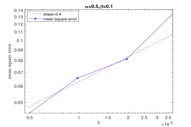
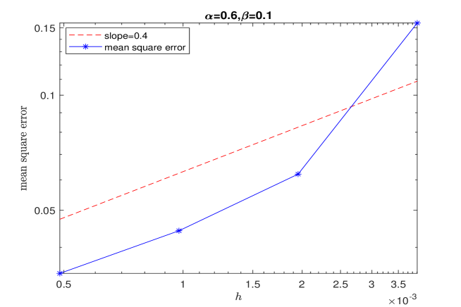
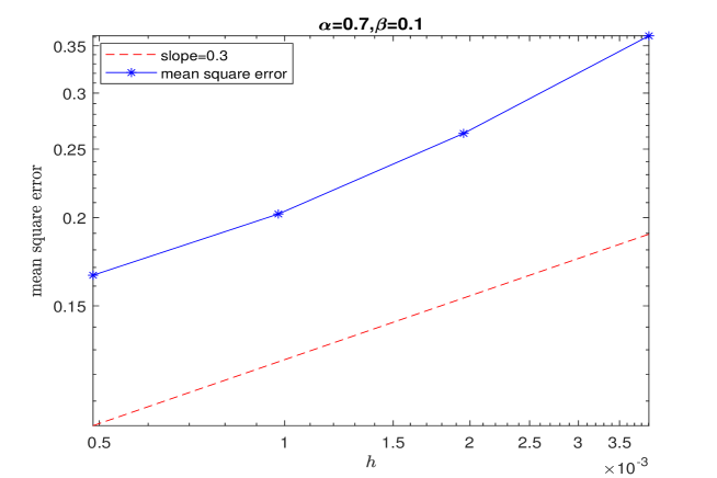
Due to appearance of the singularity in the above stochastic integral, it is difficult for us to illustrate the convergence rate of the Milstein-type scheme. Here, we only check the order of convergence of the $\theta$-EM scheme numerically. We regard the numerical solution yielded by small stepsize $h^{*}=2^{-13}$ as ’exact’ solution. Moreover, the corresponding numerical solutions are generated by four different stepsizes $h=4h^{*},8h^{*},16h^{*}$ and $32h^{*}$, respectively. The mean square errors of $\theta$-EM scheme are calculated at the terminal time $t_{N}=T=1$ by

$$e=\bigg{(}\frac{1}{M}\sum_{i=1}^{M}|X_{T}^{(i)}-X_{N}^{(i)}|^{2}\bigg{)}^{\frac{1}{2}},$$

where the expectation is approximated by averaging over $M=1000$ Brownian sample paths. The mean square errors are plotted in Figs. 1, 2, 3 in log-log scale. In these plots, the reference lines and error lines are parallel to each other, revealing the convergence rate of $\theta$-EM scheme is $\min\{1-\alpha,\frac{1}{2}-\beta\}$.

7 Conclusion

Our aim in this work is to investigate a $\theta$-Euler-Maruyama scheme and a Milstein type scheme for SVIEs with weakly singular kernels. Since Itô formula is not available, the classical proof techniques are no longer used. Our new strategy is based on the Taylor formula, classical fractional calculus, and discrete and continuous typed Gronwall inequalities with weakly singular kernels. The convergence rates of these schemes have been given by a technical analysis on the equation the solution satisfies. And the convergence results of $\theta$-Euler-Maruyama scheme are demonstrated through some numerical experiments. In forthcoming works, we study a Milstein- type method for SVIEs with diagonal and boundary singularities of the kernel (cf. [17, 18, 19]). Our future work is to verify whether the order of convergence is optimal. In addition, we will study how to effectively model the multiple stochastic singular integrals.

References

- [1] D. T. Son, P. T. Huong, P. E. Kloeden, H. T. Tuan, Asymptotic separation between solutions of Caputo fractional stochastic differential equations, Stoch. Anal. Appl. 36 (4) (2018) 654–664.
- [2] P. T. Anh, T. S. Doan, P. T. Huong, A variation of constant formula for Caputo fractional stochastic differential equations, Statist. Probab. Lett. 145 (2019) 351–358.
- [3] M. Abouagwa, J. Li, Approximation properties for solutions to Itô-Doob stochastic fractional differential equations with non-Lipschitz coefficients, Stoch. Dyn. 19 (4) (2019) 1950029, 21.
- [4] M. Abouagwa, J. Li, Stochastic fractional differential equations driven by Lévy noise under Carathéodory conditions, J. Math. Phys. 60 (2) (2019) 022701, 16.
- [5] C. Tudor, M. Tudor, Approximation schemes for Itô-Volterra stochastic equations, Bol. Soc. Mat. Mexicana (3) 1 (1) (1995) 73–85.
- [6] C. H. Wen, T. S. Zhang, Improved rectangular method on stochastic Volterra equations, J. Comput. Appl. Math. 235 (8) (2011) 2492–2501.
- [7] Y. Wang, Approximate representations of solutions to SVIEs, and an application to numerical analysis, J. Math. Anal. Appl. 449 (1) (2017) 642–659.
- [8] Y. Xiao, J. N. Shi, Z. W. Yang, Split-step collocation methods for stochastic Volterra integral equations, J. Integral Equations Appl. 30 (1) (2018) 197–218.
- [9] H. Liang, Z. Yang, J. Gao, Strong superconvergence of the Euler-Maruyama method for linear stochastic Volterra integral equations, J. Comput. Appl. Math. 317 (2017) 447–457.
- [10] J. Gao, H. Liang, S. Ma, Strong convergence of the semi-implicit Euler method for nonlinear stochastic Volterra integral equations with constant delay, Appl. Math. Comput. 348 (2019) 385–398.
- [11] H. Yang, Z. Yang, S. Ma, Theoretical and numerical analysis for Volterra integro-differential equations with Itô integral under polynomially growth conditions, Appl. Math. Comput. 360 (2019) 70–82.
- [12] W. Zhang, H. Liang, J. Gao, Theoretical and numerical analysis of the Euler-Maruyama method for generalized stochastic Volterra integro-differential equations, J. Comput. Appl. Math. 365 (2020) 112364, 17.
- [13] W. Zhang, Theoretical and numerical analysis of a class of stochastic Volterra integro-differential equations with non-globally Lipschitz continuous coefficients, Appl. Numer. Math. 147 (2020) 254–276.
- [14] X. Dai, W. Bu, A. Xiao, Well-posedness and EM approximations for non-Lipschitz stochastic fractional integro-differential equations, J. Comput. Appl. Math. 356 (2019) 377–390.
- [15] H. Brunner, Collocation methods for Volterra integral and related functional differential equations, Vol. 15 of Cambridge Monographs on Applied and Computational Mathematics, Cambridge University Press, Cambridge, 2004.
- [16] R. Gorenflo, A. A. Kilbas, F. Mainardi, S. V. Rogosin, Mittag-Leffler functions, related topics and applications, Springer Monographs in Mathematics, Springer, Heidelberg, 2014.
- [17] A. Pedas, G. Vainikko, Integral equations with diagonal and boundary singularities of the kernel, Z. Anal. Anwend. 25 (4) (2006) 487–516.
- [18] M. Kolk, A. Pedas, Numerical solution of Volterra integral equations with weakly singular kernels which may have a boundary singularity, Math. Model. Anal. 14 (1) (2009) 79–89.
- [19] X. Dai, A. Xiao, Lévy-driven stochastic Volterra integral equations with doubly singular kernels: existence, uniqueness, and a fast EM method, Adv. Comput. Math. 46 (2).