Predictable Accelerator Design
with Time-Sensitive Affine Types

Abstract.

Field-programmable gate arrays (FPGAs) provide an opportunity to co-design applications with hardware accelerators, yet they remain difficult to program. High-level synthesis (HLS) tools promise to raise the level of abstraction by compiling C or C++ to accelerator designs. Repurposing legacy software languages, however, requires complex heuristics to map imperative code onto hardware structures. We find that the black-box heuristics in HLS can be unpredictable: changing parameters in the program that should improve performance can counterintuitively yield slower and larger designs. This paper proposes a type system that restricts HLS to programs that can predictably compile to hardware accelerators. The key idea is to model consumable hardware resources with a time-sensitive affine type system that prevents simultaneous uses of the same hardware structure. We implement the type system in Dahlia, a language that compiles to HLS C++, and show that it can reduce the size of HLS parameter spaces while accepting Pareto-optimal designs.

1. Introduction

While Moore’s law may not be dead yet, its stalled returns for traditional CPUs have sparked renewed interest in specialized hardware accelerators (Hennessy and Patterson, 2019), for domains from machine learning (Jouppi et al., 2017) to genomics (Turakhia et al., 2018). Reconfigurable hardware—namely, field-programmable gate arrays (FPGAs)—offer some of the benefits of specialization without the cost of custom silicon. FPGAs can accelerate code in domains from databases (Chung et al., 2013) to networking (Arashloo et al., 2020) and have driven vast efficiency improvements in Microsoft’s data centers (Putnam et al., 2014; Fowers et al., 2018).

However, FPGAs are hard to program. The gold-standard programming model for FPGAs is register transfer level (RTL) design in hardware description languages such as Verilog, VHDL, Bluespec, and Chisel (Nikhil, 2004; Bachrach et al., 2012). RTL requires digital design expertise: akin to assembly languages for CPUs, RTL is irreplaceable for manual performance tuning, but it is too explicit and verbose for rapid iteration (Sutherland et al., 2007).

FPGA vendors offer high-level synthesis (HLS) or “C-to-gates” tools (Xilinx Inc., [n.d.]b; Cong et al., 2011; Pilato and Ferrandi, 2013; Canis et al., 2011) that translate annotated subsets of C and C++ to RTL. Repurposing a legacy software languages, however, has drawbacks: the resulting language subset is small and difficult to specify, and minor code edits can cause large swings in hardware efficiency. We find empirically that smoothly changing source-level hints can cause wild variations in accelerator performance. Semantically, there is no HLS programming language: there is only the subset of C++ that a particular version of a particular compiler supports.

This paper describes a type system that restricts HLS to programs whose hardware implementation is clear. The goal is predictable architecture generation: the hardware implications are observable in the source code, and costly implementation decisions require explicit permission from the programmer. Instead of silently generating bad hardware for difficult input programs, the type system yields errors that help guide the programmer toward a better design. The result is a language that can express a subset of the architectures that HLS can—but it does so predictably.

The central insight is that an affine type system (Tov and Pucella, 2011) can model the restrictions of hardware implementation. Components in a hardware design are finite and expendable: a subcircuit or a memory can only do one thing at a time, so a program needs to avoid conflicting uses. Previous research has shown how to apply substructural type systems to model classic computational resources such as memory allocations and file handles (Grossman et al., 2002; Bernardy et al., 2017; Matsakis and Klock, 2014; Tov and Pucella, 2011) and to enforce exclusion for safe shared-memory parallelism (Gordon et al., 2012; Baker, 1995; Clebsch et al., 2015). Unlike those classic resources, however, the availability of hardware components changes with time. We extend affine types with time sensitivity to express that repeated uses of the same hardware is safe as long as they are temporally separated.

We describe Dahlia, a programming language for predictable accelerator design. Dahlia differs from traditional HLS in two ways: (1) Dahlia makes the hardware implementation for each language construct manifest in the source code instead of leaving this decision up to the HLS middle-end, and (2) Dahlia uses its time-sensitive affine types to reason about the hardware constraints and reject programs that would require complex transformation to implement in hardware. We implement a compiler for Dahlia that emits annotated C++ for a commercial HLS toolchain. We show that predictability pitfalls exist in both industrial and recent academic tools and that Dahlia’s reasoning can help alleviate these issues.

The contributions of this paper are:

• We identify predictability pitfalls in HLS and measure their effects in an industrial tool in Section 2.

• We design Dahlia (Section 3), a language that restricts HLS to predictable design spaces by modeling hardware constraints using time-sensitive affine types.

• We formalize a time-sensitive affine type system and prove syntactic type soundness in Section 4.

• We empirically demonstrate Dahlia’s effectiveness in rejecting unpredictable design points and its ability to make area–performance trade-offs in common accelerator designs in Section 5.

2. Predictability Pitfalls in Traditional HLS

Figure 1. Overview of a traditional high-level synthesis toolchain and how Dahlia layers type safety on top.

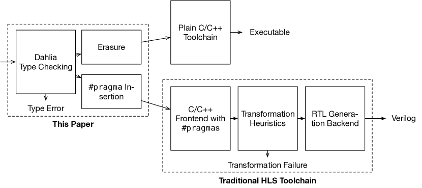
Figure 1 depicts the design of a traditional high-level synthesis (HLS) compiler. A typical HLS tool adopts an existing open-source C/C++ frontend and adds a set of transformation heuristics that attempt to map software constructs onto hardware elements along with a backend that generates RTL code (Cong et al., 2006; Canis et al., 2011). The transformation step typically relies on a constraint solver, such as an LP or SAT solver, to satisfy resource, layout, and timing requirements (Gupta et al., 2004; Cong and Zhang, 2006). Programmers can add #pragma hints to guide the transformation—for example, to duplicate loop bodies or to share functional units.

HLS tools are best-effort compilers: they make a heuristic effort to translate any valid C/C++ program to RTL, regardless of the consequences for the generated accelerator architecture. Sometimes, the mapping constraints are unsatisfiable, so the compiler selectively ignores some #pragma hints or issues an error. The generated accelerator’s efficiency depends on the interaction between the code, the hints, and the transformation heuristics that use them.

The standard approach prioritizes automation over predictability. Small code changes can yield large shifts in the generated architecture. When performance is poor, the compiler provides little guidance about how to improve it. Pruning such unpredictable points from the design space would let programmers explore smaller, smoother parameter spaces.

2.1. An Example in HLS

⬇

int m1[512][512], m2[512][512], prod[512][512];

int sum;

for (int i = 0; i < 512; i++) {

for (int j = 0; j < 512; j++) {

sum = 0;

for (int k = 0; k < 512; k++) {

sum += m1[i][k] * m2[k][j];

}

prod[i][j] = sum; } }

Figure 2. Dense matrix multiplication in HLS-friendly C.

(a) The original code.

(b) With unrolling.

(c) With unrolling and banking.

Figure 3. Three accelerator implementations of the matrix multiplication in Figure 2.

(a) Unrolling without partitioning.

(b) Unrolling with 8-way partitioning.

(c) Unrolling and banking in lockstep.

Figure 4. Look-up table count (top) and execution latency (bottom) for the kernel in Figure 2 with varying parameters.

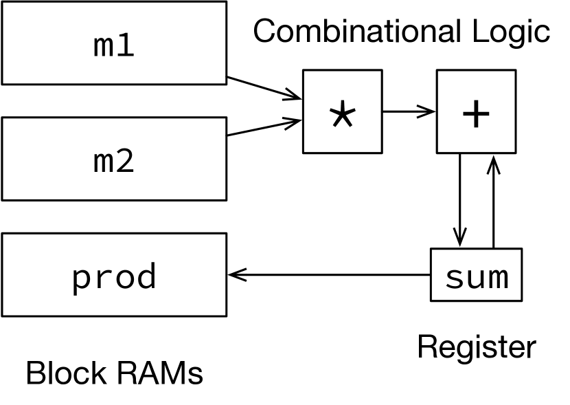
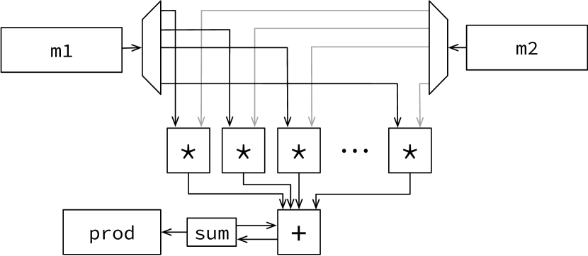
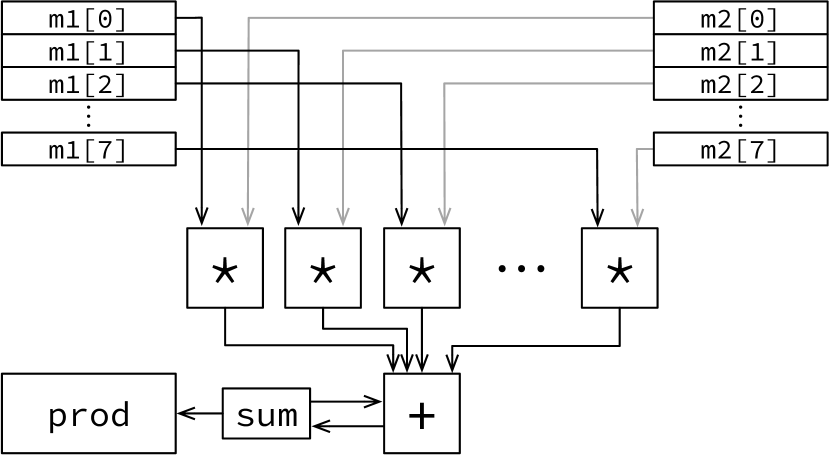
Programming with HLS centers on arrays and loops, which correspond to memory banks and logic blocks. Figure 2 shows the C code for a matrix multiplication kernel. This section imagines the journey of a programmer attempting to use HLS to generate a fast FPGA-based accelerator from this code. We use Xilinx’s SDAccel (Xilinx Inc., [n.d.]a) compiler (v2018.3.op) and target an UltraScale+ VU9P FGPA on an AWS F1 instance (Amazon Web Services, [n.d.]) to perform the experiments in this section.

Initial accelerator.

Our imaginary programmer might first try compiling the code verbatim. The HLS tool maps the arrays m1, m2, and prod onto on-chip memories. FPGAs have SRAM arrays, called block RAMs (BRAMs), that the compiler allocates for this purpose. The loop body becomes combinational logic consisting of a multiplier, an adder, and an accumulator register. Figure 3(a) depicts this configuration.

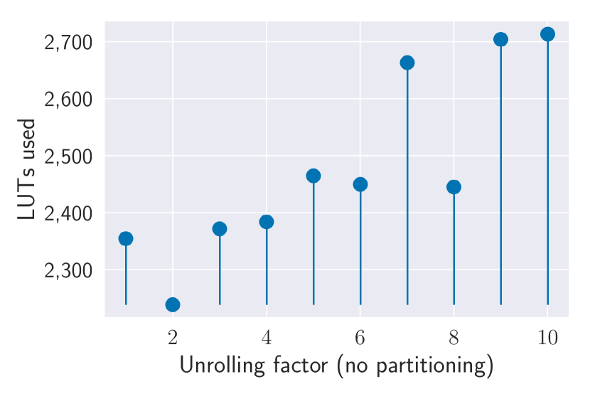
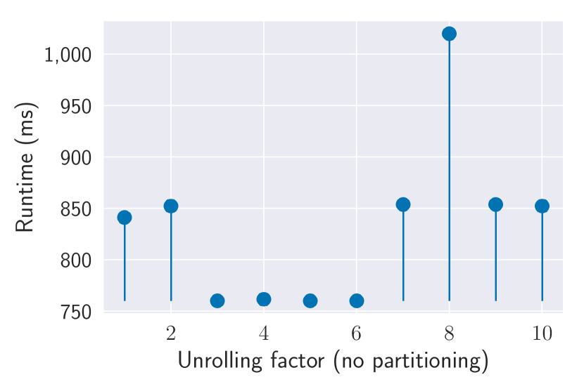
This design, while functional, does not harness any parallelism that an FPGA can offer. The two key metrics for evaluating an accelerator design are performance and area, i.e., the amount of physical chip resources that the accelerator occupies. This initial configuration computes the matrix product in 841.1 ms and occupies 2,355 of the device’s lookup tables (LUTs). However, the target FPGA device has over 1 million LUTs, so the programmer’s next job is to expend more of the FPGA area to improve performance.

Loop unrolling.

The standard tool that HLS offers for expressing parallelism is an UNROLL annotation, which duplicates the logic for a loop body. A programmer might attempt to obtain a better accelerator design by adding this annotation to the innermost loop on lines 6–8 in Figure 2:

⬇

#pragma HLS UNROLL FACTOR=8

This unrolling directive instructs the HLS tool to create 8 copies of the multiplier and adder, called processing elements (PEs), and attempt to run them in parallel. Loop unrolling represents an area–performance trade-off: programmers can reasonably expect greater unrolling factors to consume more of the FPGA chip but yield lower-latency execution.

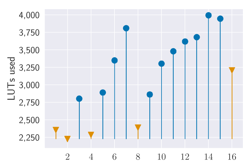
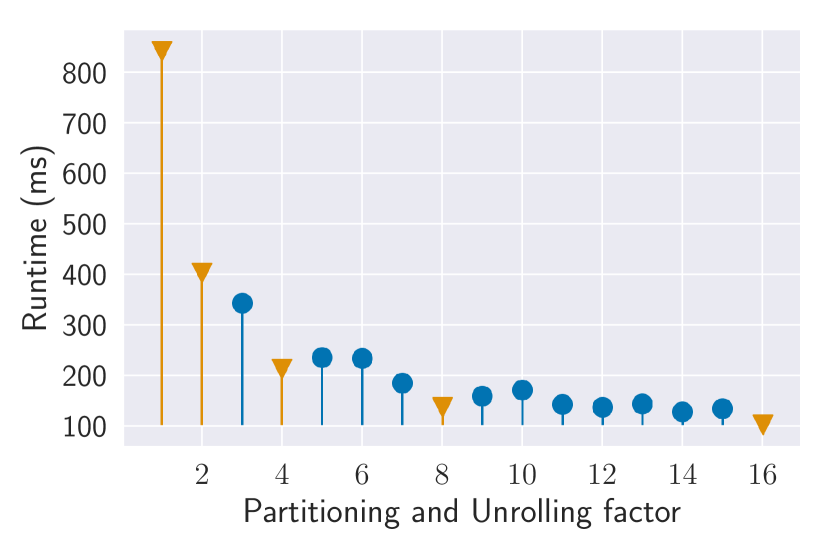
The UNROLL directive alone, however, fails to achieve this objective. Figure 4(a) shows the effect of various unrolling factors on this code in area (LUT count) and performance (latency). There is no clear trend: greater unrolling yields unpredictably better and worse designs. The problem is that the accelerator’s memories now bottleneck the parallelism provided by the PEs. The BRAMs in an FPGA have a fixed, small number of ports, so they can only service one or two reads or writes at a time. So while the HLS tool obeys the programmer’s UNROLL request to duplicate PEs, its scheduling must serialize their execution. Figure 3(b) shows how the HLS tool must insert additional multiplexing hardware to connect the multipliers to the single-ported memories. The additional hardware and the lack of parallelism yields the unpredictable performance and area for different PE counts.

Memory banking to match parallelism.

To achieve expected speedups from parallelism, accelerators need to use multiple memories. HLS tools provide annotations to partition arrays, allocating multiple BRAMs and increasing the access throughput. The programmer can insert these partitioning annotations to allocate 8 BRAMs per input memory:

⬇

#pragma HLS ARRAY_PARTITION VARIABLE=m1 FACTOR=8

#pragma HLS ARRAY_PARTITION VARIABLE=m2 FACTOR=8

Banking uses several physical memories, each of which stores a subset of the array’s data. The compiler partitions the array using a “round-robin” policy to enable parallel access. In this example, elements 0 and 8 go in bank 0, elements 1 and 9 go in bank 1, etc.:

(Each shade represents a different memory bank.) Figure 3(c) shows the resulting architecture, which requires no multiplexing and allows memory parallel access.

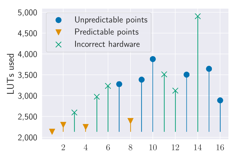
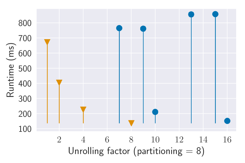
Combining banking and unrolling, however, unearths another source of unpredictable performance. While the HLS tool produces a good result when both the banking factors and the loop unrolling factor are 8, other design choices perform worse. Figure 4(b) shows the effect of varying the unrolling factor while keeping the arrays partitioned with factor 8. Again, the area and performance varies unpredictably with the unrolling factor. Reducing the unrolling factor from 9 to 8 can counter-intuitively improve both performance and area. In our experiments, some unrolling factors yield hardware that produces incorrect results. (We show the area but omit the running time for these configurations.)

The problem is that some partitioning/unrolling combinations yield much simpler hardware than others. When both the unrolling and the banking factors are 8, each parallel PE need only access a single bank, as in Figure 3(c). The first PE needs to access elements 0, 8, 16, and so on—and because the array elements are “striped” across the banks, all of these values live in the first bank. With unrolling factor 9, however, the first PE needs to access values from every bank, which requires complicated memory indirection hardware. With unrolling factor 4, the indirection cost is smaller—the first PE needs to access only bank 0 and bank 4.

From the programmer’s perspective, the HLS compiler silently enforces an unwritten rule: When the unrolling factor divides the banking factor, the area is good and parallelism predictably improves performance. Otherwise, all bets are off. Figure 4(b) labels the points where the unrolling factor divides the banking factor as predictable points. The HLS compiler emits no errors or warnings for any parameter setting.

Banking vs. array size.

Even if we imagine that a programmer carefully ensures that banking factors exactly match unrolling factors, another pitfall awaits them when choosing the amount of parallelism. Figure 4(c) shows the effects of varying the banking and unrolling factor in our kernel together. The LUT count again varies wildly.

The problem is that, when the banking and unrolling factors do not evenly divide the sizes of the arrays involved, the accelerator needs extra hardware to cope with the “leftover” elements. The memory banks are unevenly sized, and the PEs need extra hardware to selectively disable themselves on the final iteration to avoid out-of-bounds memory accesses.

Again, there is a predictable subset of design points when the programmer obeys the unwritten rule: An array’s banking factor should divide the array size. Figure 4(c) highlights the predictable points that follow this rule. Among this subset, the performance reliably improves with increasing parallelism and the area cost scales proportionally.

2.2. Enforcing the Unwritten Rules

The underlying problem in each of these sources of unpredictability is that the traditional HLS tool prioritizes automation over programmer control. While automation can seem convenient, mapping heuristics give rise to implicit rules that, when violated, silently produce bad hardware instead of reporting a useful error.

This paper instead prioritizes the predictability of hardware generation and making architectural decisions obvious in the source code. HLS tools already contain such a predictable subset hidden within their unrestricted input language. By modeling resource constraints, we can separate out this well-behaved fragment. Figure 1 shows how our checker augments a traditional HLS toolchain by lifting hidden compiler reasoning into the source code and rejecting potentially unpredictable programs.

The challenge, however, is that the “unwritten rules” of HLS are never explicitly encoded anywhere—they arise implicitly from non-local interactions between program structure, hints, and heuristics. A naïve syntactic enforcement strategy would be too conservative—it would struggle to allow flexible, fine-grained sharing of hardware resources.

We design a type system that models the constraints of hardware implementation to enforce these constraints in a composable, formal way. Our type system addresses target-independent issues—it prevents problems that would occur even on an arbitrarily large FPGA. We do not attempt to rule out resource exhaustion problems because they would tie programs to specific target devices. We see that kind of quantitative resource reasoning as important future work.

3. The Dahlia Language

Dahlia’s type system enforces a safety property: that the number of simultaneous reads and writes to a given memory bank may not exceed the number of ports. While traditional HLS tools enforce this requirement with scheduling heuristics, Dahlia enforces it at the source level using types.

The key ideas in Dahlia are (1) using substructural typing to reason about consumable hardware resources and (2) expressing time ordering in the language to reason about when resources are available. This section describes these two core features (Sections 3.1 and 3.2) and then shows how Dahlia builds on them to yield a language that is flexible enough to express real programs (Sections 3.3, 3.4, 3.5 and 3.6).

3.1. Affine Memory Types

The foundation of Dahlia’s type system is its reasoning about memories. The problem in Section 2.1’s example is conflicting simultaneous accesses to the design’s memories. The number of reads and writes supported by a memory per cycle is limited by the number of ports in the memory. HLS tools automatically detect potential read/write conflicts and schedule accesses across clock cycles to avoid errors. Dahlia instead makes this reasoning about conflicts explicit by enforcing an affine restriction on memories.

Memories are defined by giving their type and size:

⬇

let A: float[10];

The type of A is mem float[10], denoting a single-ported memory that holds 10 floating-point values. Each Dahlia memory corresponds to an on-chip BRAM in the FPGA. Memories resemble C or Java arrays: programs read and mutate the contents via subscripting, as in A[5] := 4.2. Because they represent static physical resources in the generated hardware, memory types differ from plain value types like float by preventing duplication and aliasing:

⬇

let x = A[0]; // OK: x is a float.

let B = A; // Error: cannot copy memories.

The affine restriction on memories disallows reads and writes to a memory that might occur at the same time:

⬇

let x = A[0]; // OK

A[1] := 1; // Error: Previous read consumed A.

While type-checking A, the Dahlia compiler removes A from the typing context. Subsequent uses of A are errors, with one exception: identical reads to the same memory location are allowed. This program is valid, for example:

⬇

let x = A[0];

let y = A[0]; // OK: Reading the same address.

The type system uses access capabilities to check reads and writes (Fluet et al., 2006; Gordon et al., 2013). A read expression such as A[0] acquires a non-affine read capability for index $0$ in the current scope, which permits unlimited reads to the same location but prevents the acquisition of other capabilities for A. The generated hardware reads once from A and distributes the result to both variables x and y, as in this equivalent code:

⬇

let tmp = A[0]; let x = tmp; let y = tmp;

However, memory writes use affine write capabilities, which are use-once resources: multiple simultaneous writes to the same memory location remain illegal.

3.2. Ordered and Unordered Composition

A key HLS optimization is parallelizing execution of independent code. This optimization lets HLS compilers parallelize and reorder dependency-free statements connected by ; when the hardware constraints allow it—critically, when they do not need to access the same memory banks.

Dahlia makes these parallelism opportunities explicit by distinguishing between ordered and unordered composition. The C-style ; connector is unordered: the compiler is free to reorder and parallelize the statements on either side while respecting their data dependencies. A second connector, ---, is ordered: in A --- B, statement A must execute before B.

Dahlia prevents resource conflicts in unordered composition but allows two statements in ordered composition to use the same resources. For example, Dahlia accepts this program that would be illegal when joined by the ; connector:

⬇

let x = A[0]

---

A[1] := 1

In the type checker, ordered composition restores the affine resources that were consumed in the first command before checking the second command. The capabilities for all memories are discarded, and the program can acquire fresh capabilities to read and write any memory.

Together, ordered and unordered composition can express complex concurrent designs:

⬇

let A: float[10]; let B: float[10];

{

let x = A[0] + 1

---

B[1] := A[1] + x // OK

};

let y = B[0]; // Error: B already consumed.

The statements composed with --- are ordered with each other but unordered with the last line. The read therefore must not conflict with either of the first two statements.

Logical time.

From the programmer’s perspective, a chain of ordered computations executes over a series of logical time steps. Logical time in Dahlia does not directly reflect physical time (i.e., clock cycles). Instead, the HLS backend is responsible for allocating cycles to logical time steps in a way that preserves the ordering of memory accesses. For example, a long logical time step containing an integer division might require multiple clock cycles to complete, and the compiler may optimize away unneeded time steps that do not separate memory accesses. Regardless of optimizations, however, a well-typed Dahlia program requires at least enough ordered composition to ensure that memory accesses do not conflict.

Local variables as wires & registers.

Local variables, defined using the let construct, do not share the affine restrictions of memories. Programs can freely read and write to local variables without restriction, and unordered composition respects the dependencies induced by local variables:

⬇

let x = 0; x := x + 1; let y = x; // All OK

In hardware, local variables manifest as wires or registers. The choice depends on the allocation of physical clock cycles: values that persist across clock cycles require registers. Consider this example consisting of two logical time steps:

⬇

let x = A[0] + 1 --- B[0] := A[1] + x

The compiler must implement the two logical time steps in different clock cycles, so it must use a register to hold x. In the absence of optimizations, registers appear whenever a variable’s live range crosses a logical time step boundary. Therefore, programmers can minimize the use of registers by reducing the live ranges of variables or by reducing the amount of sequential composition.

3.3. Memory Banking

As Section 2.1 details, HLS tools can bank memories into disjoint components to allow parallel access. Dahlia memory declarations support bank annotations:

⬇

let A: float[8 bank 4];

In a memory type mem $t$[$n$ bank $m$], the banking factor $m$ must evenly divide the size $n$ to yield equally-sized banks. HLS tools, in contrast, allow uneven banking and silently insert additional hardware to account for it (see Section 2.1).

Affine restrictions for banks.

Dahlia tracks an affine resource for each memory bank. To physically address a bank, the syntax $M${$b$}[$i$] denotes the $i$th element of $M$’s $b$th bank. This program is legal, for example:

⬇

let A: float[10 bank 2];

A{0}[0] := 1;

A{1}[0] := 2; // OK: Accessing a different bank.

Dahlia also supports logical indexing into banked arrays using the syntax $M$[$n$] for literals $n$. For example, A[1] is equivalent to A{1}[0] above. Because the index is static, the type checker can automatically deduce the bank and offset.

Multi-ported memories.

Dahlia also supports reasoning about multi-ported memories. This syntax declares a memory where each bank has two read/write ports:

⬇

let A: float{2}[10];

A memory provides $k$ affine resources per bank where $k$ is the number of ports in a memory. This rule lets multi-ported memories provide multiple read/write capabilities in each logical time step. For example, Dahlia accepts this program:

⬇

let A: float{2}[10];

let x = A[0];

A[1] := x + 1;

Dahlia does not guarantee data-race freedom in the presence of multi-ported memories. Programs are free to write to and read from the same memory location in the same logical time step and should expect the semantics of the underlying memory technology. Extensions to rule out data races would resemble race detection for parallel software (Pratikakis et al., 2006; Naik et al., 2006).

Multi-dimensional banking.

Banking generalizes to multi-dimensional arrays. Every dimension can have an independent banking factor. This two-dimensional memory has two banks in each dimension, a total of $2\times 2=4$ banks:

⬇

let M: float[4 bank 2][4 bank 2];

The physical and logical memory access syntax similarly generalizes to multiple dimensions. For example, M{3}[0] represents the element logically located at M[1][1].

3.4. Loops and Unrolling

Fine-grained parallelism is an essential optimization in hardware accelerator design. Accelerator designers duplicate a block of logic to trade off area for performance: $n$ copies of the same logic consume $n$ times as much area while offering a theoretical $n$-way speedup. Dahlia syntactically separates parallelizable doall for loops, which must not have any cross-iteration dependencies, from sequential while loops, which may have dependencies but are not parallelizable. Programmers can mark for loops with an unroll factor to duplicate the loop body logic and run it in parallel:

⬇

for (let i = 0..10) unroll 2 { f(i) }

This loop is equivalent to a sequential one that iterates half as many times and composes two copies of the body in parallel:

⬇

for (let i = 0..5) { f(2*i + 0); f(2*i + 1) }

The doall restriction is important because it allows the compiler to run the two copies of the loop body in parallel using unordered composition. In traditional HLS tools, a loop unrolling annotation such as #pragma HLS unroll is always allowed—even when the loop body makes parallelization difficult or impossible. The toolchain will replicate the loop body and rely on complex analysis and resource scheduling to optimize the unrolled loop body as well as it can.

Resource conflicts in unrolled loops are errors. For example, this loop accesses an unbanked array in parallel:

⬇

let A: float[10];

for (let i = 0..10) unroll 2 {

A[i] := compute(i) // Error: Insufficient banks.

}

Unrolled memory accesses.

Dahlia uses special index types for loop iterators to type-check memory accesses within unrolled loops. Index types generalize integers to encode information about loop unrolling. In this example:

⬇

for (let i = 0..8) unroll 4 { A[i] }

The iterator i gets the type idx{0..4}, indicating that accessing an array at i will consume banks 0, 1, 2, and 3. Type-checking a memory access with i consumes all banks indicated by its index type.

Unrolling and ordered composition.

Loop unrolling has a subtle interaction with ordered composition. In a loop body containing ---, like this:

⬇

let A: float[10 bank 2];

for (let i = 0..10) unroll 2 {

let x = A[i]

---

f(x, A[0]) }

A naive interpretation would use parallel composition to join the loop bodies at the top level:

⬇

for (let i = 0..5) {

{ let x0 = A[2*i] --- f(x0, A[0]) };

{ let x1 = A[2*i + 1] --- f(x1, A[0]) } }

However, this interpretation is too restrictive. It requires all time steps in each loop body to avoid conflicts with all other time steps. This example would be illegal because the access to A[i] in the first time step may conflict with the access to A[0] in the second time step. Instead, Dahlia reasons about unrolled loops in lockstep by parallelizing within each logical time step. The loop above is equivalent to:

⬇

for (let i = 0..5) {

{ let x0 = A[2*i]; let x1 = A[2*i + 1] }

---

{ f(x0, A[0]); f(x1, A[0]) } }

The lockstep semantics permits this unrolling because conflicts need only be avoided between unrolled copies of the same logical time step. HLS tools must enforce a similar restriction but leave the choice to black-box heuristics.

Nested unrolling.

In nested loops, unrolled iterators can separately access dimensions of a multi-dimensional array. Nested loops also interact with Dahlia’s read and write capabilities. In this program:

⬇

let A: float[8 bank 4][10 bank 5];

for (let i = 0..8) {

for (let j = 0..10) unroll 5 {

let x = A[i][0]

---

A[i][0] := j; // Error: Insufficient write

} } // capabilities.

The read to array $A[i][0]$ can be proved to be safe because after desugaring, the reads turn into:

⬇

let x0 = A[i][0]; let x1 = A[i][0] ...

The access is safe because the first access acquires a read capability for indices i and 0, so the subsequent copies are safe. Architecturally, the code entails a single read fanned out to each parallel PE. However, the write desugars to:

⬇

A[i][0] := j; A[i][0] := j + 1 ...

which causes a write conflict in the hardware.

3.5. Combine Blocks for Reduction

In traditional HLS, loops can freely include dependent operations, as in this dot product:

⬇

for (let i = 0..10) unroll 2 { dot += A[i] * B[i] }

However, the += update silently introduces a dependency between every iteration which is disallowed by Dahlia’s doall for-loops. HLS tools heuristically analyze loops to extract and serialize dependent portions. In Dahlia, programmers explicitly distinguish the non-parallelizable reduction components of for loops. Each for can have an optional combine block that contains sequential code to run after each unrolled iteration group of the main loop body. For example, this loop is legal:

⬇

for (let i = 0..10)

unroll 2 {

let v = A[i] * B[i];

} combine {

dot += v;

}

There are two copies of the loop body that run in parallel and feed into a single reduction tree for the combine block.

The type checker gives special treatment to variables like v that are defined in for bodies and used in combine blocks. In the context of the combine block, v is a combine register, which is a tuple containing all values produced for v in the unrolled loop bodies. Dahlia defines a class of functions called reducers that take a combine register and return a single value (similar to a functional fold). Dahlia defines +=, -=, *=, /= as built-in reducers with infix syntax.

3.6. Memory Views for Flexible Iteration

(a) No view.

(b) Shrink view.

(c) Suffix view.

(d) Shift view.

(e) Split view.

Figure 5. Hardware schematics for each kind of memory view. Highlighted outlines indicate added hardware cost.

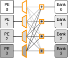
In order to predictably generate hardware for parallel accesses, Dahlia statically calculates banks accessed by each PE and guarantees that they are distinct. Figure 5(a) shows the kind of hardware generated by this restriction—each PE is directly connected to a bank.

To enforce this hardware generation, Dahlia only allows simple indexing expressions like A[i] and A[4] and rejects arbitrary index calculations like A[2*i]. General indexing expressions can require complex indirection hardware to allow any PE to access any memory bank. An access like A[i*i], for example, makes it difficult to deduce which bank it would read on which iteration. For simple expressions like A[j+8], however, the bank stride pattern is clear. Traditional HLS tools make a best-effort attempt to deduce access patterns, but subtle changes in the code can unpredictable prevent the analysis and generate bad hardware.

Dahlia uses memory views to define access patterns that HLS compilers can compile efficiently and to convince the Dahlia type checker that a parallel access will be predictable. The key idea is to offer different logical arrangements of the same underlying physical memory. By logically re-organizing the memory, views can simply reuse Dahlia’s type-checking to ensure that complex access patterns are predictable. Furthermore, this allows views to capture the hardware cost of an access pattern in the source code instead of relying on black-box analysis in HLS tools. For Dahlia’s HLS C++ backend, views are compiled to direct memory accesses.

The rest of this section describes Dahlia’s memory views and their cost in terms of hardware required to transform bank and index values to support the iteration pattern.

Shrink.

To directly connect PEs to memory banks, Dahlia requires the unrolling factor to match the banking factor. To allow lower unrolling factors, Dahlia provides shrink views, which reduce the banking factors of an underlying memory by an integer factor. For example:

⬇

let A: float[8 bank 4];

view sh = shrink A[by 2]; // sh: float[8 bank 2]

for (let i = 0..8) unroll 2

sh[i]; // OK: sh has 2 banks. Compiled to: A[i].

The example first defines a view sh with the underlying memory A and divides its banking factor by 2. Dahlia allows sh[i] here because each PE will access a distinct set of banks. The first PE accesses banks 0 and 2; the second accesses banks 1 and 3. The hardware cost of a shrink view, as Figure 5(b) illustrates, consists of multiplexing to select the right bank on every iteration. The access sh[i] compiles to A[i].

Suffix.

A second kind of view lets programs create small slices of a larger memory. Dahlia distinguishes between suffixes that it can implement efficiently and costlier ones. An efficient aligned suffix view uses this syntax:

⬇

view v = suffix M[by $k$ * $e$];

where view v starts at element $k\times e$ of the memory M. Critically, $k$ must be the banking factor of M. This restriction allows Dahlia to prove that each logical bank in the view maps to the same physical bank while the indices are offset by the indexing expression. The hardware cost of a suffix view is the address adapter for each bank. A view access v{$b$}[$i$] is compiled to M{$b$}[$e+i$].

For example, generating suffixes in a loop results in this pattern, where the digits in each cell are the indices, the shades represent the banks, and the highlighted outline indicates the view:

⬇

let A: float[8 bank 2];

for (let i = 0..4) {

view s = suffix A[by 2*i];

s[1]; // reads A[2*i + 1]

}

A suffix view defined using view v = suffix M[by k*e] and accessed using v[i] is compiled to M[k*e + i].

Shift.

Shifted suffixes are like standard suffixes but allow unrestricted offset expressions:

⬇

view v = shift M[by e];

Since e is unrestricted, Dahlia assumes that both the bank and the indices need to be adapted and that each PE accesses every bank. Figure 5(d) shows the hardware cost of a shift view: each PE is connected to every bank and the index expression is transformed using an address adapter. The distinction between suffix and shift views allows Dahlia to capture the cost of different accessing schemes.

Even in this worst-case scenario, Dahlia can reason about the disjointness of bank accesses. This loop is legal:

⬇

let A: float[12 bank 4];

for (let i = 0..3) {

view r = shift A[by i*i]; // r: float[12 bank 4]

for (let j = 0..4) unroll 4

let x = r[j]; // accesses A[i*i + j]

}

The view r has a memory type, so Dahlia can guarantee that the inner access r[j] uses disjoint banks and is therefore safe to parallelize. An access r[$i$] to a view declared with shift M[by $e$] compiles to M[$e+i$].

Split.

Some nested iteration patterns can be parallelized at two levels: globally, over an entire array, and locally, over a smaller window. This pattern arises in blocked computations, such as this dot product loop in C++:

⬇

float A[12], B[12], sum = 0.0;

for (int i = 0; i < 6; i++)

for (int j = 0; j < 2; j++)

sum += A[2*i + j] * B[2*i + j];

Both the inner loop and the outer loop represent opportunities for parallelization. However, Dahlia cannot prove this parallelization to be safe:

⬇

let A, B: float[12 bank 4];

view shA, shB = shrink A[by 2], B[by 2];

for (let i = 0..6) unroll 2 {

view vA, vB = suffix shA[by 2*i], shB[by 2*i];

for (let j = 0..2) unroll 2 {

let v = vA[j] + vB[j];

} combine {

sum += v; }}

While Dahlia can prove that the inner accesses into the views can be predictably parallelized, it cannot establish the disjointness of the parallel copies of the views va and vb created by the outer unrolled loop.

Split views allow for this reasoning. The key idea is to create logically more dimensions than the physical memory and reusing Dahlia’s reasoning for multidimensional memories to prove safety for such parallel accesses. A split view transforms a one-dimensional memory (left) into a two-dimensional memory (right):

Using these split-view declarations:

⬇

view split_A = split A[by 2];

view split_B = split B[by 2];

Each view has type mem float[2 bank 2][6 bank 2]. A row in the logical view represents a “window” for computation. The above example can now unroll both loops, by changing the inner access to:

⬇

let v = split_A[j][i] * split_B[j][i];

As Figure 5(e) illustrates, split views have similar cost to aligned suffix views: they require no bank indirection hardware because the bank index is always known statically. They require an address adapter to compute the address within the bank from the separate coordinates. A split view declared view sp = split M[by $k$] on a memory M with $k$ banks translates the access sp[$i$][$j$] to M{bank}[idx] where:

$$\text{bank}=i*k+(j\bmod b)\quad\text{idx}=\left\lfloor\dfrac{j}{b}\right\rfloor$$

4. Formalism

$$x \in\text{variables}\enspace\enspace a\in\text{memories}\enspace\enspace n\in\text{numbers}$$

$$b ::=\mathbf{true}\mid\mathbf{false}\qquad v::=n\mid b$$

$$e ::=v\mid\mathbf{bop}\;e_{1}\;e_{2}\mid x\mid a[e]$$

$$c ::=e\mid\mathbf{let}\;x=e\mid c_{1}~{}\rule[1.93748pt]{13.50002pt}{0.55pt}~{}c_{2}\mid c_{1}~{}\textbf{;}~{}c_{2}\mid\mathbf{if}\;x\;c_{1}\;c_{2}\mid$$

$$\qquad\mathbf{while}\;x\;c\mid x:=e\mid a[e_{1}]:=e_{2}\mid\mathbf{skip}$$

$$\tau ::=\mathbf{bit}\langle n\rangle\mid\mathbf{float}\mid\mathbf{bool}\mid\mathbf{mem}\;\tau[n_{1}]$$

Figure 6. Abstract syntax for the Filament core language.

This section formalizes the time-sensitive affine type system that underlies Dahlia in a core language, Filament. We give both a large-step semantics, which is more intelligible, and a small-step semantics, which enables a soundness proof.

4.1. Syntax

Figure 6 lists the grammar for Filament. Filament statements $c$ resemble a typical imperative language: there are expressions, variable declarations, conditions, and simple sequential iteration via while. Filament has ordered composition $c_{1}~{}\rule[2.15277pt]{15.00002pt}{0.55pt}~{}c_{2}$ and unordered composition $c_{1}~{}\textbf{;}~{}c_{2}$. It separates memories $a$ and variables $x$ into separate syntactic categories. Filament programs can only declare the latter: a program runs with a fixed set of available memories.

4.2. Large-Step Semantics

Filament’s large-step operational semantics is a checked semantics that enforces Dahlia’s safety condition by explicitly tracking and getting stuck when it would otherwise require two conflicting accesses. Our type system (Section 4.3) aims to rule out these conflicts.

The semantics uses an environment $\sigma$ mapping variable and memory names to values, which may be primitive values or memories, which in turn map indices to primitive values. A second context, $\rho$, is the set of the memories that the program has accessed. $\rho$ starts empty and accumulates memories as the program reads and writes them.

The operational semantics consists of an expression judgment $\sigma_{1},\rho_{1},e\Downarrow\sigma_{2},\rho_{2},v$ and a command judgment $\sigma_{1},\rho_{1},c\Downarrow\sigma_{2},\rho_{2}$. We describe some relevant rules here, and the supplementary material lists the full semantics and proof (Nigam et al., [n.d.]).

Memory accesses.

Memories in Filament are mutable stores of values. Banked memories in Dahlia can be built up using these simpler memories. The rule for a memory read expression $a[n]$ requires that $a$ not already be present in $\rho$, which would indicate that the memory was previously consumed:

$$\displaystyle{\hbox{\hskip 85.58357pt\vbox{\hbox{\hskip-85.58357pt\hbox{\hbox{$\displaystyle\displaystyle\mathit{a}\not\in\rho_{{\mathrm{1}}}\qquad\sigma_{{\mathrm{1}}},\rho_{{\mathrm{1}}},\mathit{e}\Downarrow\sigma_{{\mathrm{2}}},\rho_{{\mathrm{2}}},\mathit{n}\qquad\sigma_{{\mathrm{2}}}(a)(n)=\mathit{v}$}}}\vbox{}}}\over\hbox{\hskip 45.9609pt\vbox{\vbox{}\hbox{\hskip-45.9609pt\hbox{\hbox{$\displaystyle\displaystyle\sigma_{{\mathrm{1}}},\rho_{{\mathrm{1}}},\mathit{a}[\mathit{e}]\Downarrow\sigma_{{\mathrm{2}}},\rho_{{\mathrm{2}}}\cup\{\mathit{a}\},\mathit{v}$}}}}}}$$

Composition.

Unordered composition accumulates the resource demands of two commands by threading $\rho$ through:

$$\displaystyle{\hbox{\hskip 63.69174pt\vbox{\hbox{\hskip-63.69174pt\hbox{\hbox{$\displaystyle\displaystyle\sigma_{{\mathrm{1}}},\rho_{{\mathrm{1}}},\mathit{c_{{\mathrm{1}}}}\Downarrow\sigma_{{\mathrm{2}}},\rho_{{\mathrm{2}}}\qquad\sigma_{{\mathrm{2}}},\rho_{{\mathrm{2}}},\mathit{c_{{\mathrm{2}}}}\Downarrow\sigma_{{\mathrm{3}}},\rho_{{\mathrm{3}}}$}}}\vbox{}}}\over\hbox{\hskip 34.8528pt\vbox{\vbox{}\hbox{\hskip-34.8528pt\hbox{\hbox{$\displaystyle\displaystyle\sigma_{{\mathrm{1}}},\rho_{{\mathrm{1}}},\mathit{c_{{\mathrm{1}}}}~{}\textbf{;}~{}\mathit{c_{{\mathrm{2}}}}\Downarrow\sigma_{{\mathrm{3}}},\rho_{{\mathrm{3}}}$}}}}}}$$

If both commands read or write the same memory, they will conflict in $\rho$. Ordered composition runs each command in the same initial $\rho$ environment and merges the resulting $\rho$:

$$\displaystyle{\hbox{\hskip 63.69174pt\vbox{\hbox{\hskip-63.69174pt\hbox{\hbox{$\displaystyle\displaystyle\sigma_{{\mathrm{1}}},\rho_{{\mathrm{1}}},\mathit{c_{{\mathrm{1}}}}\Downarrow\sigma_{{\mathrm{2}}},\rho_{{\mathrm{2}}}\qquad\sigma_{{\mathrm{2}}},\rho_{{\mathrm{1}}},\mathit{c_{{\mathrm{2}}}}\Downarrow\sigma_{{\mathrm{3}}},\rho_{{\mathrm{3}}}$}}}\vbox{}}}\over\hbox{\hskip 47.93939pt\vbox{\vbox{}\hbox{\hskip-47.93938pt\hbox{\hbox{$\displaystyle\displaystyle\sigma_{{\mathrm{1}}},\rho_{{\mathrm{1}}},\mathit{c_{{\mathrm{1}}}}~{}\rule[1.93748pt]{13.50002pt}{0.55pt}~{}\mathit{c_{{\mathrm{2}}}}\Downarrow\sigma_{{\mathrm{3}}},\rho_{{\mathrm{2}}}\cup\rho_{{\mathrm{3}}}$}}}}}}$$

4.3. Type System

The typing judgments have the form $\Gamma_{{\mathrm{1}}},\Delta_{{\mathrm{1}}}\vdash\mathit{c}\dashv\Gamma_{{\mathrm{2}}},\Delta_{{\mathrm{2}}}$ and $\Gamma,\Delta_{{\mathrm{1}}}\vdash\mathit{e}:\tau\dashv\Delta_{{\mathrm{2}}}$. $\Gamma$ is a standard typing context for variables and $\Delta$ is the affine context for memories.

Affine memory accesses.

Memories are affine resources. The rules for reads and writes check the type of the index in $\Gamma$ and remove the memory from $\Delta$:

$$\displaystyle{\hbox{\hskip 89.97874pt\vbox{\hbox{\hskip-89.97874pt\hbox{\hbox{$\displaystyle\displaystyle\Gamma,\Delta_{{\mathrm{1}}}\vdash\mathit{e_{{\mathrm{1}}}}:\mathbf{bit}\langle\mathit{n}\rangle\dashv\Delta_{{\mathrm{2}}}\qquad\Delta_{{\mathrm{2}}}=\Delta_{{\mathrm{3}}}\cup\{\mathit{a}\mapsto\mathbf{mem}\,\tau[\mathit{n_{{\mathrm{1}}}}]\}$}}}\vbox{}}}\over\hbox{\hskip 34.79973pt\vbox{\vbox{}\hbox{\hskip-34.79973pt\hbox{\hbox{$\displaystyle\displaystyle\Gamma,\Delta_{{\mathrm{1}}}\vdash\mathit{a}[\mathit{e}]:\tau\dashv\Delta_{{\mathrm{3}}}$}}}}}}$$

Composition.

The unordered composition rule checks the first statement in the initial contexts and uses the resulting contexts to check the second statement:

$$\displaystyle{\hbox{\hskip 73.3501pt\vbox{\hbox{\hskip-73.3501pt\hbox{\hbox{$\displaystyle\displaystyle\Gamma_{{\mathrm{1}}},\Delta_{{\mathrm{1}}}\vdash\mathit{c_{{\mathrm{1}}}}\dashv\Gamma_{{\mathrm{2}}},\Delta_{{\mathrm{2}}}\qquad\Gamma_{{\mathrm{2}}},\Delta_{{\mathrm{2}}}\vdash\mathit{c_{{\mathrm{2}}}}\dashv\Gamma_{{\mathrm{3}}},\Delta_{{\mathrm{3}}}$}}}\vbox{}}}\over\hbox{\hskip 39.68198pt\vbox{\vbox{}\hbox{\hskip-39.68198pt\hbox{\hbox{$\displaystyle\displaystyle\Gamma_{{\mathrm{1}}},\Delta_{{\mathrm{1}}}\vdash\mathit{c_{{\mathrm{1}}}}~{}\textbf{;}~{}\mathit{c_{{\mathrm{2}}}}\dashv\Gamma_{{\mathrm{3}}},\Delta_{{\mathrm{3}}}$}}}}}}$$

Ordered composition checks both commands under the same resource set, $\Delta_{1}$, but threads the non-affine context through:

$$\displaystyle{\hbox{\hskip 73.3501pt\vbox{\hbox{\hskip-73.3501pt\hbox{\hbox{$\displaystyle\displaystyle\Gamma_{{\mathrm{1}}},\Delta_{{\mathrm{1}}}\vdash\mathit{c_{{\mathrm{1}}}}\dashv\Gamma_{{\mathrm{2}}},\Delta_{{\mathrm{2}}}\qquad\Gamma_{{\mathrm{2}}},\Delta_{{\mathrm{1}}}\vdash\mathit{c_{{\mathrm{2}}}}\dashv\Gamma_{{\mathrm{3}}},\Delta_{{\mathrm{3}}}$}}}\vbox{}}}\over\hbox{\hskip 54.192pt\vbox{\vbox{}\hbox{\hskip-54.192pt\hbox{\hbox{$\displaystyle\displaystyle\Gamma_{{\mathrm{1}}},\Delta_{{\mathrm{1}}}\vdash\mathit{c_{{\mathrm{1}}}}~{}\rule[1.93748pt]{13.50002pt}{0.55pt}~{}\mathit{c_{{\mathrm{2}}}}\dashv\Gamma_{{\mathrm{3}}},\Delta_{{\mathrm{2}}}\cap\Delta_{{\mathrm{3}}}$}}}}}}$$

The rule merges the resulting $\Delta$ contexts with set intersection to yield the resources not consumed by either statement.

4.4. Small-Step Semantics

We also define a small-step operational semantics for Filament upon which we build a proof of soundness. We claim that the small-step semantics, when iterated to a value, is equivalent to the big-step semantics. The semantics consists of judgments $\sigma_{{\mathrm{1}}},\rho_{{\mathrm{1}}},\mathit{e}\rightarrow\sigma_{{\mathrm{2}}},\rho_{{\mathrm{2}}},\mathit{e^{\prime}}$ and $\sigma_{{\mathrm{1}}},\rho_{{\mathrm{1}}},\mathit{c}\rightarrow\sigma_{{\mathrm{2}}},\rho_{{\mathrm{2}}},\mathit{c^{\prime}}$ where $\sigma$ and $\rho$ are the environment and the memory context respectively. The main challenge is sequential composition, which uses an intermediate command form $\smash{c_{1}\overset{\rho}{\sim}c_{2}}$ to thread $\rho$ to $c_{1}$ and $c_{2}$. The supplementary material has full details.

4.5. Desugaring Surface Constructs

Filament desugars surface language features present in Dahlia.

Memory banking.

A banked memory declaration like this:

⬇

let A: float[$m$ bank $n$];

desugars into several unbanked memories:

⬇

let A_0: float[$\frac{m}{n}$]; let A_1: float[$\frac{m}{n}$]; ...

Desugaring transforms reads and writes of banked memories to conditional statements that use the indexing expression to decide which bank to access.

Loop unrolling.

Desugaring of for loops uses the technique described in Section 3.4, translating from:

⬇

for (let i = 0 .. $m$) unroll $k$ { $c_{1}$ --- $c_{2}$ ... }

into a while loop that duplicates the body:

⬇

let i = 0;

while (i < $\frac{m}{k}$) {

{ $c_{1}[$i$\;\mapsto\;$k*i+0$]$; $c_{1}[$i$\;\mapsto\;$k*i+1$]$ ... }

---

{ $c_{2}[$i$\;\mapsto\;$k*i+0$]$; $c_{2}[$i$\;\mapsto\;$k*i+1$]$ ... }

...

i++; }

where $c[x\mapsto e]$ denotes substitution.

Memory views.

For views’ operational semantics, a desugaring based on the mathematical descriptions in Section 3.6 suffices. To type-check them, however, would require tracking the underlying memory for each view (transitively, to cope with views of views) and type-level reasoning about the bank requirements of an access pattern. Formal treatment of these types would require an extension to Filament.

Multi-ported memories.

Reasoning about memory ports requires quantitative resource tracking, as in bounded linear logic (Girard et al., 1992). We leave such an extension of Filament’s affine type system as future work.

4.6. Soundness Theorem

We state a soundness theorem for Filament’s type system with respect to its checked small-step operational semantics.

Theorem 0.

If $\emptyset,\Delta^{*}\vdash c\dashv\Gamma_{2},\Delta_{2}$ and $\emptyset,\emptyset,c\stackrel{{\scriptstyle*}}{{\rightarrow}}\sigma,\rho,c^{\prime}$ and $\sigma,\rho,c^{\prime}\mathchoice{\mathrel{\hbox to0.0pt{\kern 2.5pt\kern-5.27776pt$\displaystyle\not$\hss}{\rightarrow}}}{\mathrel{\hbox to0.0pt{\kern 2.5pt\kern-5.27776pt$\textstyle\not$\hss}{\rightarrow}}}{\mathrel{\hbox to0.0pt{\kern 1.75pt\kern-4.11108pt$\scriptstyle\not$\hss}{\rightarrow}}}{\mathrel{\hbox to0.0pt{\kern 1.25pt\kern-3.3333pt$\scriptscriptstyle\not$\hss}{\rightarrow}}}$, then $c^{\prime}=\text{\bf{skip}}$.

where $\Delta^{*}$ is the initial affine context of memories available to a program. The theorem states that a well-typed program never gets stuck due to memory conflicts in $\rho$. We prove this theorem using progress and preservation lemmas:

Lemma 1 (Progress).

If $\Gamma,\Delta\vdash c\dashv\Gamma_{2},\Delta_{2}$ and $\Gamma,\Delta\sim\sigma,\rho$, then $\sigma,\rho,c\rightarrow\sigma^{\prime},\rho^{\prime},c^{\prime}$ or $c=\text{\bf{skip}}$.

Lemma 2 (Preservation).

If $\Gamma,\Delta\vdash c\dashv\Gamma_{2},\Delta_{2}$ and $\Gamma,\Delta\sim\sigma,\rho$, and $\sigma,\rho,c\rightarrow\sigma^{\prime},\rho^{\prime},c^{\prime}$, then $\Gamma^{\prime},\Delta^{\prime}\vdash c^{\prime}\dashv\Gamma_{2}^{\prime},\Delta_{2}^{\prime}$ and $\Gamma^{\prime},\Delta^{\prime}\sim\sigma^{\prime},\rho^{\prime}$.

In these lemmas, $\Gamma,\Delta\sim\sigma,\rho$ is a well-formedness judgment stating that all variables in $\Gamma$ are in $\sigma$ and all memories in $\Delta$ are not in $\rho$. Using an extension of the syntax in Figure 6, we prove the lemmas by induction on the small-step relation (Nigam et al., [n.d.]).

5. Evaluation

Our evaluation measures whether Dahlia’s restrictions can improve predictability without sacrificing too much sheer performance. We conduct two experiments: (1) We perform an exhaustive design space exploration for one kernel to determine how well the restricted design points compare to the much larger unrestricted parameter space. (2) We port the MachSuite benchmarks (Reagen et al., 2014) and, where Dahlia yields a meaningful design space, perform a parameter sweep.

5.1. Implementation and Experimental Setup

We implemented a Dahlia compiler in 5200 LoC of Scala. The compiler checks Dahlia programs and generates C++ code using Xilinx Vivado HLS’s #pragma directives (Xilinx Inc., [n.d.]b). We execute benchmarks on AWS F1 instances (Amazon Web Services, [n.d.]) with 8 vCPUs, 122 GB of main memory, and a Xilinx UltraScale+ VU9P. We use the SDAccel development environment (Xilinx Inc., [n.d.]a) and synthesize the benchmarks with a target clock period of 250 MHz.

5.2. Case Study: Unrestricted DSE vs. Dahlia

(a) Pareto-optimal points.

(b) Points accepted by Dahlia.

(c) Cluster of Pareto points.

Figure 7. Results from exhaustive design space exploration for gemm-blocked.

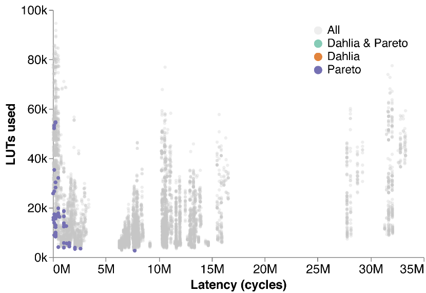
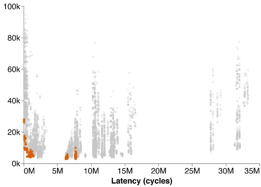
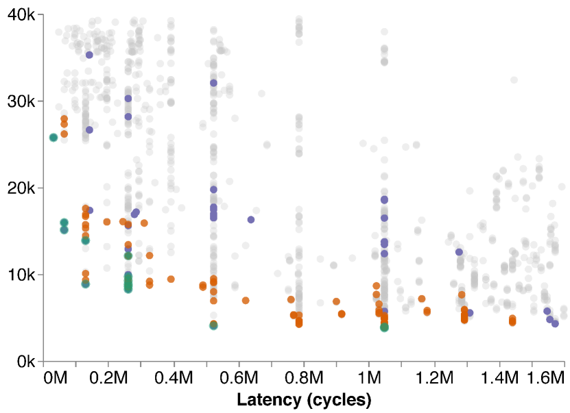
In this section, we conduct an exhaustive design-space exploration (DSE) of a single benchmark as a case study. Without Dahlia, the HLS design space is extremely large—we study how the smaller Dahlia-restricted design space compares. We select a blocked matrix multiplication kernel (gemm-blocked from MachSuite) for its large but tractable design space. The kernel has 3 two-dimensional arrays (two operands and the output product) and 5 nested loops, of which the inner 3 are parallelizable. We define parameters for the 6 banking factors (two dimensions for each memory) and 3 unrolling factors. (A full code listing appears in the supplementary material (Nigam et al., [n.d.]).) We explore a design space with banking factors of 1–4 and unrolling factors of 1, 2, 4, 6, and 8. This design space consists of 32,000 distinct configurations.

We exhaustively evaluated the entire design space using Vivado HLS’s estimation mode, which required a total of 2,666 compute hours. We identify Pareto-optimal configurations according to their estimated cycle latency and number of lookup tables (LUTs), flip flops (FFs), block RAMs (BRAMs), and arithmetic units (DSPs).

Dahlia accepts 354 configurations, or about 1.1% of the unrestricted design space. But the smaller space is only valuable if it consists of useful design points—a broad range of Pareto-optimal configurations. Figures 7(a) and 7(b) show the Pareto-optimal points and the subset of points that Dahlia accepts, respectively. (Pareto optimality is determined using all objectives, but the plot shows only two: LUTs and latency.) Figure 7(c) shows a zoomed-in view of the tight cluster of Pareto points in the bottom-left of the first two graphs. Dahlia-accepted points lie primarily on the Pareto frontier and allow area-latency trade-offs. The optimal points that Dahlia rejects expend a large number of LUTs to reduce BRAM consumption which, while Pareto optimal, don’t seem to be of practical use.

5.3. Dahlia-Directed DSE & Programmability

We port benchmarks from an HLS benchmark suite, MachSuite (Reagen et al., 2014), to study Dahlia’s flexibility. Of the 19 MachSuite benchmarks, one (backprop) contains a correctness bug and two fail to synthesize correctly in Vivado, indicating a bug in the tools. We successfully ported all 16 of the remaining benchmarks without substantial restructuring.

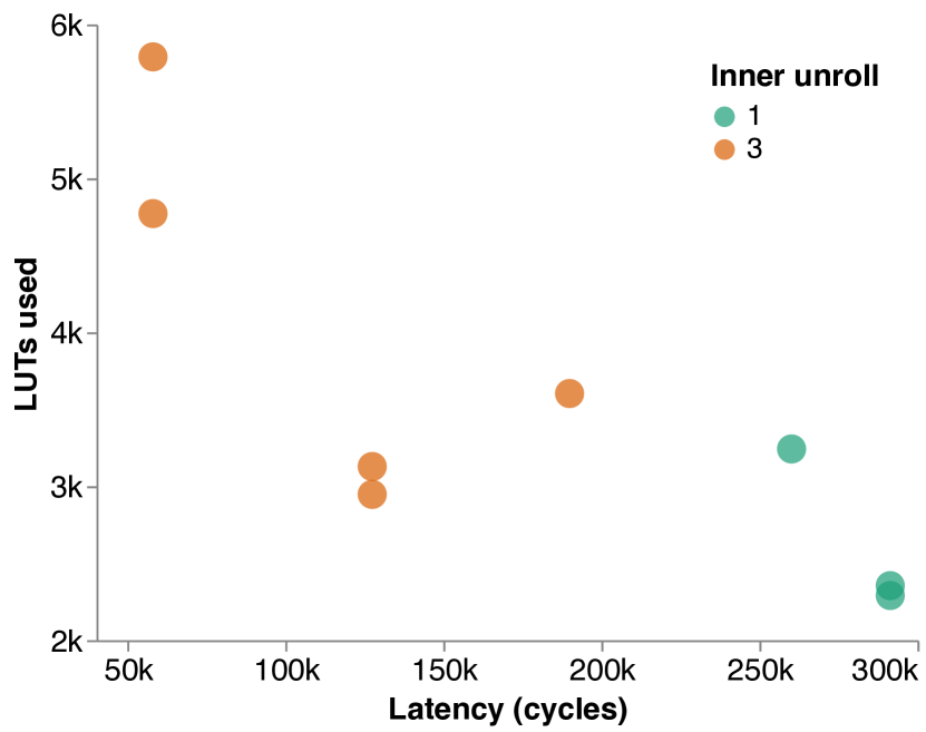
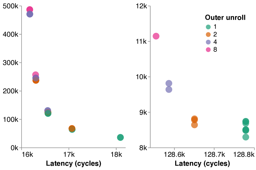
From these, we select 3 benchmarks that exhibit the kind of fine-grained, loop-level parallelism that Dahlia targets as case studies: sencil2d, md-knn, and md-grid. As the previous section illustrates, an unrestricted DSE is intractable for even modestly sized benchmarks, so we instead measure the breadth and performance of the much smaller space of configurations that Dahlia accepts. For each benchmark, we find all optimization parameters available in the Dahlia port and define a search space. The type checker rejects some design points, and we measure the remaining space. We use Vivado HLS’s estimation mode to measure the resource counts and estimated latency for each accepted point. Figure 8 depicts the Pareto-optimal points in each space. In each plot, we also highlight the effect a single parameter has on the results.

The rest of this section reports quantitatively on each benchmark’s design space and reports qualitatively on the programming experience during the port from C to Dahlia.

(a) stencil2d with inner unroll.

(b) md-knn with outer unroll.

(c) md-grid with middle unroll.

Figure 8. The design spaces for three MachSuite benchmarks. Each uses a color to highlight one design parameter.

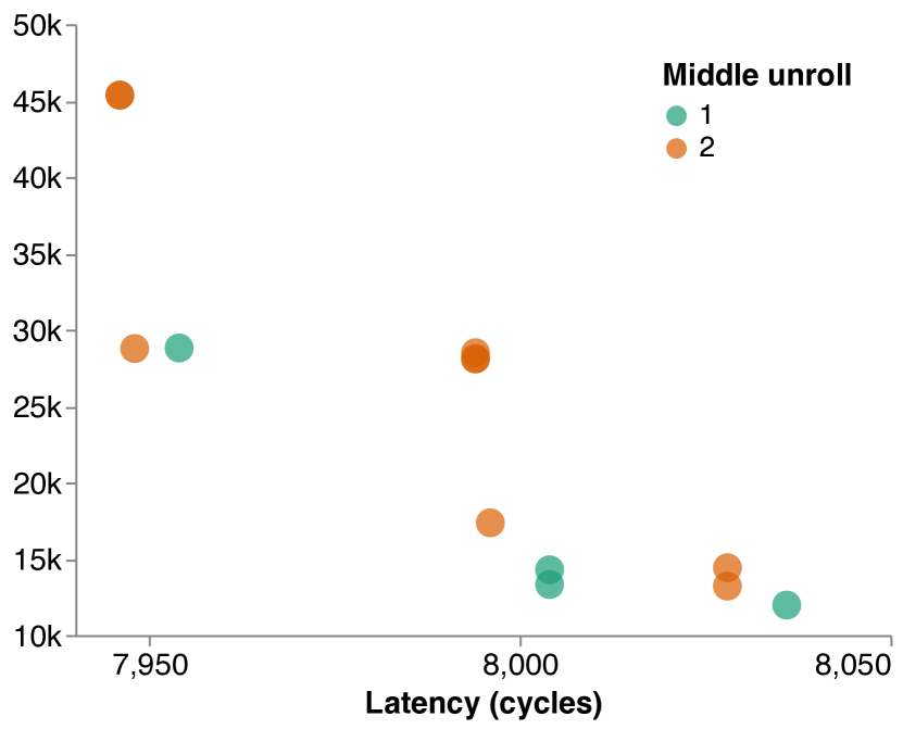
stencil2d.

MachSuite’s stencil2d is a filter operation with four nested loops. The outer loops scan over the input matrix and the inner loops apply a $3\times 3$ filter. Our Dahlia port unrolls the inner two loops and banks both input memories. We use unrolling factors from 1 to 3 and bank each dimension of the input array by factors 1 to 6. The resulting design space has 2,916 points. Dahlia accepts 18 of these points (0.6%), of which 8 are Pareto-optimal within the set.

Figure 8(a) shows the Pareto frontier among the Dahlia-accepted points. The figure uses color to show the unrolling factor for the innermost loop. This unrolling factor has a large effect on the design’s performance, while banking factors and the other loop explain the rest of the variation.

The original C code uses single-dimensional arrays and uses index arithmetic to treat them as matrices:

⬇

for (r=0; r<row_size-2; r++)

for (c=0; c<col_size-2; c++)

for (k1=0; k1<3; k1++)

for (k2=0; k2<3; k2++)

mul = filter[k1*3 + k2] *

orig[(r+k1)*col_size + c+k2];

In the Dahlia port, we must use proper two-dimensional arrays because the compiler rejects arbitrary indexing expressions. Using views, programmers can decouple the storage format from the iteration pattern. To express the accesses to the input matrix orig, we create a shifted suffix view (Section 3.6) for the current window:

⬇

for (let row = 0..126) {

for (let col = 0..62) {

view window = shift orig[by row][by col];

for (let k1 = 0..3) unroll 3 {

for (let k2 = 0..3) unroll 3 {

let mul = filter[k1][k2] * window[k1][k2];

The view makes the code’s logic more obvious while allowing the Dahlia type checker to allow unrolling on the inner two loops. It also clarifies why parallelizing the outer loops would be undesirable: the parallel views would require overlapping regions of the input array, introducing a bank conflict.

md-knn.

The md-knn benchmark implements an $n$-body molecular dynamics simulation with a $k$-nearest neighbors kernel. The MachSuite implementation uses data-dependent loads in its main loop, which naïvely seems to prevent parallelization. In our Dahlia port, however, we hoist this serial section into a separate loop that runs before the main, parallelizable computation. Dahlia’s type system helped guide the programmer toward a version of the benchmark where the benefits from parallelization are clear.

For each of the program’s four memories, we used banking factors from 1 to 4. We unrolled each of the two nested loops with factors from 1 to 8. The full space has 16,384 points, of which Dahlia accepts 525 (3%). 37 of the Dahlia-accepted points are Pareto-optimal.

Figure 8(b) shows two Pareto frontiers that Dahlia accepts at different scales. The color shows the unrolling factor of the outer loop. The frontier on the right uses an order of magnitude fewer resources but is an order of magnitude slower. In this kernel, the dominant effect is the memory banking (not shown in the figure), which determines which frontier the designs fall into. The outer unrolling factor (shown in color) affects the two regimes differently: on the right, it allows area–latency trade-offs within the frontier; on the left, it acts as a second-order effect that expends LUTs to achieve a small increase in performance.

md-grid.

Another algorithm for the same molecular dynamics problem, md-grid, uses a different strategy based on a 3D grid implemented with several 4-dimensional arrays. It calculates forces between neighboring grid cells. Of its 6 nested loops, the outer three are parallelizable. We use banking factors of 1 to 4 for each dimension of each array, and we try unrolling factors from 1 to 8 for both loops. The full space has 21,952 points, of which Dahlia accepts 81 (0.4%). 13 of the Dahlia-accepted points are Pareto-optimal.

Figure 8(c) again shows the Pareto-optimal design points. The innermost loop unrolling factor (not shown in the figure) determines which of three coarse regimes the design falls into. The color shows the second loop unrolling factor, which determines a second-order area–latency trade-off within each regime. Unrolling enables latency-area trade-offs in both the cases.

6. Future Work

Dahlia represents a first step toward high-level semantics for accelerator design languages. It leaves several avenues for future work on scaling up from kernels to full applications and expressing more hardware implementation techniques.

Modularity.

Dahlia’s type system relies on a closed-world assumption. A compositional type system would enable reuse of abstract hardware modules without “inlining” them, like functions in a software language. The primary challenge in modular accelerator design is the balance between abstraction and efficiency: a more general module is likely to be less efficient. An abstraction mechanism must also cope with the timing of inter-module interactions: some interfaces are latency-insensitive while others rely on cycle-level timing.

Polymorphism.

Dahlia’s memory types are monomorphic. Polymorphism would enable abstraction over memories’ banking strategies and sizes. A polymorphic Dahlia-like language could rule out invalid combinations of abstract implementation parameters before the designer picks concrete values, which would help constrain the search space for design space exploration.

Pipelining.

Pipelined logic is a critical implementation technique for high-level synthesis. Dahlia does not reason about the timing of pipeline stages or their resource conflicts. Extensions to its type system will need to reason about the cycle-level latency of these stages and track the fine-grained sharing of logic resources.

Direct RTL generation.

The current Dahlia compiler relies on a commercial C++-based HLS compiler as its backend. It generates directives that instruct the HLS tool to generate hardware according to the program’s Dahlia types, but the unpredictability of traditional HLS means that results can still vary. Future compilers for Dahlia-like languages might generate RTL directly and rely on the simpler input language avoid the complexity of unrestricted HLS.

7. Related Work

Dahlia builds on a long history of work on safe systems programming. Substructural type systems are known to be a good fit for controlling system resources  (Bernardy et al., 2017; Grossman et al., 2002; Tov and Pucella, 2011; Clebsch et al., 2015; Matsakis and Klock, 2014). Dahlia’s enforcement of exclusive memory access resembles work on race-free parallel programming using type and effect systems (Bocchino et al., 2009) or concurrent separation logic (O’Hearn, 2007). Safe parallelism on CPUs focuses on data races where concurrent reads and writes to a memory are unsynchronized. Conflicts in Dahlia are different: any simultaneous pair of accesses to the same bank is illegal. The distinction influences Dahlia’s capability system and its memory views, which cope with the arrangement of arrays into parallel memory banks.

Dahlia takes inspiration from other approaches to improving the accelerator design process, including HDLs, HLS, DSLs, and other recent accelerator design languages.

Spatial.

Figure 9. Resource utilization for gemm-ncubed in Spatial normalized to the design without unrolling.

Spatial (Koeplinger et al., 2018) is a language for designing accelerators that builds on parallel patterns (Prabhakar et al., 2016), which are flexible hardware templates. Spatial adds some automation beyond traditional HLS: it infers a banking strategy given some parallel accesses. Like HLS, Spatial designs can be unpredictable. Figure 13 shows resource usage for the matrix multiplication kernel from Section 2 written in Spatial. (A full experimental setup appears in the supplementary material (Nigam et al., [n.d.]).) For unrolling factors that do not evenly divide the memory size, Spatial will sometimes infer a banking factor that is not equal to the unrolling factor. In these cases, the resource usage abruptly increases. A type system like Dahlia could help address these predictability pitfalls in Spatial.

Better HDLs.

Modern hardware description languages (Bachrach et al., 2012; Lockhart et al., 2014; Clow et al., 2017; Baaij et al., 2010; Truong and Hanrahan, 2019; Jane Street, [n.d.]; Nikhil, 2004) aim to address the shortcomings of Verilog and VHDL. These languages target register transfer level (RTL) design. Dahlia targets a different level of abstraction and a different use case: it uses an imperative programming model and focuses exclusively on computational accelerators. Dahlia is not a good language for implementing a CPU, for example. Its focus on acceleration requires the language and semantics to more closely resemble software languages.

Traditional HLS.

Existing commercial (Xilinx Inc., [n.d.]b; Intel, [n.d.]; Mentor Graphics, [n.d.]; Cadence, [n.d.]) and academic (Putnam et al., 2008; Canis et al., 2011; Pilato and Ferrandi, 2013; Zhang et al., 2008) high-level synthesis (HLS) tools compile subsets of C, C++, OpenCL, or SystemC to RTL. While their powerful heuristics can be effective, when they fail, programmers have little insight into what went wrong or how to fix it (Liang et al., 2012). Dahlia represents an alternative approach that prioritizes programmer control over black-box optimization.

Targeting hardware from DSLs.

Compilers to FPGAs and ASICs exist for DSLs for image processing (Hegarty et al., 2014, 2016; Pu et al., 2017; Setter, [n.d.]) and machine learning (George et al., 2014; Sharma et al., 2016). Dahlia is not a DSL: it is a general language for implementing accelerators. While DSLs offer advantages in productivity and compilation for individual application domains, they do not obviate the need for general languages to fill in the gaps between popular domains, to offer greater programmer control when appropriate, and to serve as a compilation target for multiple DSLs.

Accelerator design languages.

Some recent languages also focus on general accelerator design. HeteroCL (Lai et al., 2019) uses a Halide-like (Ragan-Kelley et al., 2013) scheduling language to describe how to map algorithms onto HLS-like hardware optimizations, and T2S (Rong, 2017) similarly lets programs describe how generate a spatial implementation. Lime (Auerbach et al., 2010) extends Java to express target-independent streaming accelerators. CoRAM (Chung et al., 2011) is not a just a language; it extends FPGAs with a programmable memory interface that adapts memory accesses, akin to Dahlia’s memory views. Dahlia’s focus on predictability and type-driven design makes it unique, as far as we are aware.

8. Conclusion

Dahlia exposes predictability as a new design goal for HLS tools. Predictability comes at a cost—it can rule out design points that perform surprisingly well because of a subtle convergence of heuristics. We see these outliers as a worthy sacrifice in exchange for an intelligible programming model and robust reasoning tools. We hope to extend Dahlia’s philosophy to bring predictability to the rest of the reconfigurable hardware system stack, from the language to the LUTs.

Appendix A Semantics

The following lists the grammar for Filament, the core language of Dahlia.

$$x \in\text{variables}\enspace\enspace a\in\text{memories}\enspace\enspace n\in\text{numbers}$$

$$b ::=\mathbf{true}\mid\mathbf{false}\qquad v::=n\mid b\mid v_{1}\;\mathbf{bop}\;v_{2}$$

$$e ::=v\mid\mathbf{bop}\;e_{1}\;e_{2}\mid x\mid a[e]$$

$$c ::=e\mid\mathbf{let}\;x=e\mid c_{1}~{}\rule[1.93748pt]{13.50002pt}{0.55pt}~{}c_{2}\mid c_{1}\overset{\rho}{\sim}c_{2}\mid c_{1}~{}\textbf{;}~{}c_{2}\mid\mathbf{if}\;x\;c_{1}\;c_{2}\mid$$

$$\qquad\mathbf{while}\;x\;c\mid x:=e\mid a[e_{1}]:=e_{2}\mid\mathbf{skip}$$

$$\tau ::=\mathbf{bit}\langle n\rangle\mid\mathbf{float}\mid\mathbf{bool}\mid\mathbf{mem}\;\tau[n_{1}]$$

The large-step operational semantics listed below capture the complete evaluation of an expression or command. The environment $\sigma$ maps variables and memory names to values, and the context $\rho$ is the set of memories the program has accessed.

• $\sigma_{{\mathrm{1}}},\rho_{{\mathrm{1}}},\mathit{e}\Downarrow\sigma_{{\mathrm{2}}},\rho_{{\mathrm{2}}},\mathit{v}$ ()

$\displaystyle\displaystyle{\hbox{\hskip 105.74185pt\vbox{\hbox{\hskip-105.74184pt\hbox{\hbox{$\displaystyle\displaystyle\sigma_{{\mathrm{1}}},\rho_{{\mathrm{1}}},\mathit{e_{{\mathrm{1}}}}\Downarrow\sigma_{{\mathrm{2}}},\rho_{{\mathrm{2}}},\mathit{v_{{\mathrm{1}}}}\qquad\sigma_{{\mathrm{2}}},\rho_{{\mathrm{2}}},\mathit{e_{{\mathrm{2}}}}\Downarrow\sigma_{{\mathrm{3}}},\rho_{{\mathrm{3}}},\mathit{v_{{\mathrm{2}}}}\qquad\mathit{v_{{\mathrm{3}}}}=\mathit{v_{{\mathrm{1}}}}\,\mathbf{bop}\,\mathit{v_{{\mathrm{2}}}}$}}}\vbox{}}}\over\hbox{\hskip 44.3659pt\vbox{\vbox{}\hbox{\hskip-44.3659pt\hbox{\hbox{$\displaystyle\displaystyle\sigma_{{\mathrm{1}}},\rho_{{\mathrm{1}}},\mathbf{bop}\,\mathit{e_{{\mathrm{1}}}}\,\mathit{e_{{\mathrm{2}}}}\Downarrow\sigma_{{\mathrm{3}}},\rho_{{\mathrm{3}}},\mathit{v_{{\mathrm{3}}}}$}}}}}}$       $\displaystyle\displaystyle{\hbox{\hskip 15.76825pt\vbox{\hbox{\hskip-15.76825pt\hbox{\hbox{$\displaystyle\displaystyle\sigma(x)=\mathit{v}$}}}\vbox{}}}\over\hbox{\hskip 24.54587pt\vbox{\vbox{}\hbox{\hskip-24.54587pt\hbox{\hbox{$\displaystyle\displaystyle\sigma,\rho,\mathit{x}\Downarrow\sigma,\rho,\mathit{v}$}}}}}}$       $\displaystyle\displaystyle{\hbox{\hskip 85.58357pt\vbox{\hbox{\hskip-85.58357pt\hbox{\hbox{$\displaystyle\displaystyle\mathit{a}\not\in\rho_{{\mathrm{1}}}\qquad\sigma_{{\mathrm{1}}},\rho_{{\mathrm{1}}},\mathit{e}\Downarrow\sigma_{{\mathrm{2}}},\rho_{{\mathrm{2}}},\mathit{n}\qquad\sigma_{{\mathrm{2}}}(a)(n)=\mathit{v}$}}}\vbox{}}}\over\hbox{\hskip 45.9609pt\vbox{\vbox{}\hbox{\hskip-45.9609pt\hbox{\hbox{$\displaystyle\displaystyle\sigma_{{\mathrm{1}}},\rho_{{\mathrm{1}}},\mathit{a}[\mathit{e}]\Downarrow\sigma_{{\mathrm{2}}},\rho_{{\mathrm{2}}}\cup\{\mathit{a}\},\mathit{v}$}}}}}}$

• $\sigma_{{\mathrm{1}}},\rho_{{\mathrm{1}}},\mathit{c}\Downarrow\sigma_{{\mathrm{2}}},\rho_{{\mathrm{2}}}$ ()

$\displaystyle\displaystyle{\hbox{\hskip 29.71088pt\vbox{\hbox{\hskip-29.71086pt\hbox{\hbox{$\displaystyle\displaystyle\sigma_{{\mathrm{1}}},\rho_{{\mathrm{1}}},\mathit{e}\Downarrow\sigma_{{\mathrm{2}}},\rho_{{\mathrm{2}}},\mathit{v}$}}}\vbox{}}}\over\hbox{\hskip 45.70937pt\vbox{\vbox{}\hbox{\hskip-45.70937pt\hbox{\hbox{$\displaystyle\displaystyle\sigma_{{\mathrm{1}}},\rho_{{\mathrm{1}}},\textbf{let}~{}\mathit{x}=\mathit{e}\Downarrow\sigma_{{\mathrm{2}}}[\mathit{x}\mapsto\mathit{v}],\rho_{{\mathrm{2}}}$}}}}}}$       $\displaystyle\displaystyle{\hbox{\hskip 63.69174pt\vbox{\hbox{\hskip-63.69174pt\hbox{\hbox{$\displaystyle\displaystyle\sigma_{{\mathrm{1}}},\rho_{{\mathrm{1}}},\mathit{c_{{\mathrm{1}}}}\Downarrow\sigma_{{\mathrm{2}}},\rho_{{\mathrm{2}}}\qquad\sigma_{{\mathrm{2}}},\rho_{{\mathrm{1}}},\mathit{c_{{\mathrm{2}}}}\Downarrow\sigma_{{\mathrm{3}}},\rho_{{\mathrm{3}}}$}}}\vbox{}}}\over\hbox{\hskip 47.93939pt\vbox{\vbox{}\hbox{\hskip-47.93938pt\hbox{\hbox{$\displaystyle\displaystyle\sigma_{{\mathrm{1}}},\rho_{{\mathrm{1}}},\mathit{c_{{\mathrm{1}}}}~{}\rule[1.93748pt]{13.50002pt}{0.55pt}~{}\mathit{c_{{\mathrm{2}}}}\Downarrow\sigma_{{\mathrm{3}}},\rho_{{\mathrm{2}}}\cup\rho_{{\mathrm{3}}}$}}}}}}$       $\displaystyle\displaystyle{\hbox{\hskip 62.43175pt\vbox{\hbox{\hskip-62.43173pt\hbox{\hbox{$\displaystyle\displaystyle\sigma_{{\mathrm{1}}},\rho_{{\mathrm{1}}},\mathit{c_{{\mathrm{1}}}}\Downarrow\sigma_{{\mathrm{2}}},\rho_{{\mathrm{2}}}\qquad\sigma_{{\mathrm{2}}},\rho,\mathit{c_{{\mathrm{2}}}}\Downarrow\sigma_{{\mathrm{3}}},\rho_{{\mathrm{3}}}$}}}\vbox{}}}\over\hbox{\hskip 45.26903pt\vbox{\vbox{}\hbox{\hskip-45.26901pt\hbox{\hbox{$\displaystyle\displaystyle\sigma_{{\mathrm{1}}},\rho_{{\mathrm{1}}},\mathit{c_{{\mathrm{1}}}}\overset{\rho}{\sim}\mathit{c_{{\mathrm{2}}}}\Downarrow\sigma_{{\mathrm{3}}},\rho_{{\mathrm{2}}}\cup\rho_{{\mathrm{3}}}$}}}}}}$       $\displaystyle\displaystyle{\hbox{\hskip 63.69174pt\vbox{\hbox{\hskip-63.69174pt\hbox{\hbox{$\displaystyle\displaystyle\sigma_{{\mathrm{1}}},\rho_{{\mathrm{1}}},\mathit{c_{{\mathrm{1}}}}\Downarrow\sigma_{{\mathrm{2}}},\rho_{{\mathrm{2}}}\qquad\sigma_{{\mathrm{2}}},\rho_{{\mathrm{2}}},\mathit{c_{{\mathrm{2}}}}\Downarrow\sigma_{{\mathrm{3}}},\rho_{{\mathrm{3}}}$}}}\vbox{}}}\over\hbox{\hskip 34.8528pt\vbox{\vbox{}\hbox{\hskip-34.8528pt\hbox{\hbox{$\displaystyle\displaystyle\sigma_{{\mathrm{1}}},\rho_{{\mathrm{1}}},\mathit{c_{{\mathrm{1}}}}~{}\textbf{;}~{}\mathit{c_{{\mathrm{2}}}}\Downarrow\sigma_{{\mathrm{3}}},\rho_{{\mathrm{3}}}$}}}}}}$       $\displaystyle\displaystyle{\hbox{\hskip 72.95425pt\vbox{\hbox{\hskip-72.95425pt\hbox{\hbox{$\displaystyle\displaystyle\sigma_{{\mathrm{1}}},\rho_{{\mathrm{1}}},\mathit{e_{{\mathrm{1}}}}\Downarrow\sigma_{{\mathrm{2}}},\rho_{{\mathrm{2}}},\mathbf{true}\qquad\sigma_{{\mathrm{2}}},\rho_{{\mathrm{2}}},\mathit{c_{{\mathrm{1}}}}\Downarrow\sigma_{{\mathrm{3}}},\rho_{{\mathrm{3}}}$}}}\vbox{}}}\over\hbox{\hskip 37.85588pt\vbox{\vbox{}\hbox{\hskip-37.85588pt\hbox{\hbox{$\displaystyle\displaystyle\sigma_{{\mathrm{1}}},\rho_{{\mathrm{1}}},\mathbf{if}\,\mathit{x}\,\mathit{c_{{\mathrm{1}}}}\,\mathit{c_{{\mathrm{2}}}}\Downarrow\sigma_{{\mathrm{3}}},\rho_{{\mathrm{3}}}$}}}}}}$       $\displaystyle\displaystyle{\hbox{\hskip 73.59177pt\vbox{\hbox{\hskip-73.59175pt\hbox{\hbox{$\displaystyle\displaystyle\sigma_{{\mathrm{1}}},\rho_{{\mathrm{1}}},\mathit{e_{{\mathrm{1}}}}\Downarrow\sigma_{{\mathrm{2}}},\rho_{{\mathrm{2}}},\mathbf{false}\qquad\sigma_{{\mathrm{2}}},\rho_{{\mathrm{2}}},\mathit{c_{{\mathrm{2}}}}\Downarrow\sigma_{{\mathrm{3}}},\rho_{{\mathrm{3}}}$}}}\vbox{}}}\over\hbox{\hskip 37.85588pt\vbox{\vbox{}\hbox{\hskip-37.85588pt\hbox{\hbox{$\displaystyle\displaystyle\sigma_{{\mathrm{1}}},\rho_{{\mathrm{1}}},\mathbf{if}\,\mathit{x}\,\mathit{c_{{\mathrm{1}}}}\,\mathit{c_{{\mathrm{2}}}}\Downarrow\sigma_{{\mathrm{3}}},\rho_{{\mathrm{3}}}$}}}}}}$       $\displaystyle\displaystyle{\hbox{\hskip 71.58731pt\vbox{\hbox{\hskip-71.5873pt\hbox{\hbox{$\displaystyle\displaystyle\sigma_{{\mathrm{1}}},\rho_{{\mathrm{1}}},\mathit{e_{{\mathrm{1}}}}\Downarrow\sigma_{{\mathrm{2}}},\rho_{{\mathrm{2}}},\mathbf{true}$}\hskip 18.00003pt\hbox{\hskip-51.95782pt\hbox{\hbox{$\displaystyle\displaystyle\sigma_{{\mathrm{2}}},\rho_{{\mathrm{2}}},\mathit{c}~{}\rule[1.93748pt]{13.50002pt}{0.55pt}~{}\mathbf{while}\,\mathit{x}\,\mathit{c}\Downarrow\sigma_{{\mathrm{3}}},\rho_{{\mathrm{3}}}$}}}}}\vbox{\hbox{\hskip-51.95782pt\hbox{\hbox{$\displaystyle\displaystyle\sigma_{{\mathrm{2}}},\rho_{{\mathrm{2}}},\mathit{c}~{}\rule[1.93748pt]{13.50002pt}{0.55pt}~{}\mathbf{while}\,\mathit{x}\,\mathit{c}\Downarrow\sigma_{{\mathrm{3}}},\rho_{{\mathrm{3}}}$}}}\vbox{}}}}\over\hbox{\hskip 40.21089pt\vbox{\vbox{}\hbox{\hskip-40.21088pt\hbox{\hbox{$\displaystyle\displaystyle\sigma_{{\mathrm{1}}},\rho_{{\mathrm{1}}},\mathbf{while}\,\mathit{x}\,\mathit{c}\Downarrow\sigma_{{\mathrm{3}}},\rho_{{\mathrm{3}}}$}}}}}}$       $\displaystyle\displaystyle{\hbox{\hskip 37.24588pt\vbox{\hbox{\hskip-37.24588pt\hbox{\hbox{$\displaystyle\displaystyle\sigma_{{\mathrm{1}}},\rho_{{\mathrm{1}}},\mathit{e_{{\mathrm{1}}}}\Downarrow\sigma_{{\mathrm{2}}},\rho_{{\mathrm{2}}},\mathbf{false}$}}}\vbox{}}}\over\hbox{\hskip 40.21089pt\vbox{\vbox{}\hbox{\hskip-40.21088pt\hbox{\hbox{$\displaystyle\displaystyle\sigma_{{\mathrm{1}}},\rho_{{\mathrm{1}}},\mathbf{while}\,\mathit{x}\,\mathit{c}\Downarrow\sigma_{{\mathrm{2}}},\rho_{{\mathrm{2}}}$}}}}}}$       $\displaystyle\displaystyle{\hbox{\hskip 29.71088pt\vbox{\hbox{\hskip-29.71086pt\hbox{\hbox{$\displaystyle\displaystyle\sigma_{{\mathrm{1}}},\rho_{{\mathrm{1}}},\mathit{e}\Downarrow\sigma_{{\mathrm{2}}},\rho_{{\mathrm{2}}},\mathit{v}$}}}\vbox{}}}\over\hbox{\hskip 40.4609pt\vbox{\vbox{}\hbox{\hskip-40.46089pt\hbox{\hbox{$\displaystyle\displaystyle\sigma_{{\mathrm{1}}},\rho_{{\mathrm{1}}},\mathit{x}:=\mathit{e}\Downarrow\sigma_{{\mathrm{2}}}[\mathit{x}\mapsto\mathit{v}],\rho_{{\mathrm{2}}}$}}}}}}$       $\displaystyle\displaystyle{\hbox{\hskip 94.77837pt\vbox{\hbox{\hskip-94.77835pt\hbox{\hbox{$\displaystyle\displaystyle\sigma_{{\mathrm{1}}},\rho_{{\mathrm{1}}},\mathit{e_{{\mathrm{1}}}}\Downarrow\sigma_{{\mathrm{2}}},\rho_{{\mathrm{2}}},\mathit{n}\qquad\sigma_{{\mathrm{2}}},\rho_{{\mathrm{2}}},\mathit{e_{{\mathrm{2}}}}\Downarrow\sigma_{{\mathrm{3}}},\rho_{{\mathrm{3}}},\mathit{v}\qquad\mathit{a}\not\in\rho_{{\mathrm{3}}}$}}}\vbox{}}}\over\hbox{\hskip 64.98094pt\vbox{\vbox{}\hbox{\hskip-64.98094pt\hbox{\hbox{$\displaystyle\displaystyle\sigma_{{\mathrm{1}}},\rho_{{\mathrm{1}}},\mathit{a}[\mathit{e_{{\mathrm{1}}}}]:=\mathit{e_{{\mathrm{2}}}}\Downarrow\sigma_{{\mathrm{3}}}[\mathit{a}[\mathit{n}]\mapsto\mathit{v}],\rho_{{\mathrm{3}}}\cup\{\mathit{a}\}$}}}}}}$

The small-step operational semantics capture incremental evaluation of an expression or command and form the basis of the proof of soundness in Appendix B.

• $\sigma,\rho,\mathit{e}\rightarrow\sigma^{\prime},\rho^{\prime},\mathit{e^{\prime}}$ ()

$\displaystyle\displaystyle{\hbox{\hskip 25.62485pt\vbox{\hbox{\hskip-25.62483pt\hbox{\hbox{$\displaystyle\displaystyle\sigma,\rho,\mathit{e}\rightarrow\sigma^{\prime},\rho^{\prime},\mathit{e^{\prime}}$}}}\vbox{}}}\over\hbox{\hskip 36.37486pt\vbox{\vbox{}\hbox{\hskip-36.37485pt\hbox{\hbox{$\displaystyle\displaystyle\sigma,\rho,\mathit{a}[\mathit{e}]\rightarrow\sigma^{\prime},\rho^{\prime},\mathit{a}[\mathit{e^{\prime}}]$}}}}}}$       $\displaystyle\displaystyle{\hbox{\hskip 13.45158pt\vbox{\hbox{\hskip-13.45158pt\hbox{\hbox{$\displaystyle\displaystyle\mathit{a}\not\in\rho$}}}\vbox{}}}\over\hbox{\hskip 41.42091pt\vbox{\vbox{}\hbox{\hskip-41.42091pt\hbox{\hbox{$\displaystyle\displaystyle\sigma,\rho,\mathit{a}[\mathit{n}]\rightarrow\sigma,\rho\cup\{\mathit{a}\},\mathit{v}$}}}}}}$       $\displaystyle\displaystyle{\hbox{\hskip 26.88484pt\vbox{\hbox{\hskip-26.88484pt\hbox{\hbox{$\displaystyle\displaystyle\sigma,\rho,\mathit{e_{{\mathrm{1}}}}\rightarrow\sigma^{\prime},\rho^{\prime},\mathit{e^{\prime}_{{\mathrm{1}}}}$}}}\vbox{}}}\over\hbox{\hskip 51.1549pt\vbox{\vbox{}\hbox{\hskip-51.1549pt\hbox{\hbox{$\displaystyle\displaystyle\sigma,\rho,\mathbf{bop}\,\mathit{e_{{\mathrm{1}}}}\,\mathit{e_{{\mathrm{2}}}}\rightarrow\sigma^{\prime},\rho^{\prime},\mathbf{bop}\,\mathit{e^{\prime}_{{\mathrm{1}}}}\,\mathit{e_{{\mathrm{2}}}}$}}}}}}$       $\displaystyle\displaystyle{\hbox{\hskip 26.88484pt\vbox{\hbox{\hskip-26.88484pt\hbox{\hbox{$\displaystyle\displaystyle\sigma,\rho,\mathit{e_{{\mathrm{2}}}}\rightarrow\sigma^{\prime},\rho^{\prime},\mathit{e^{\prime}_{{\mathrm{2}}}}$}}}\vbox{}}}\over\hbox{\hskip 51.90492pt\vbox{\vbox{}\hbox{\hskip-51.90492pt\hbox{\hbox{$\displaystyle\displaystyle\sigma,\rho,\mathbf{bop}\,\mathit{v_{{\mathrm{1}}}}\,\mathit{e_{{\mathrm{2}}}}\rightarrow\sigma^{\prime},\rho^{\prime},\mathbf{bop}\,\mathit{v_{{\mathrm{1}}}}\,\mathit{e^{\prime}_{{\mathrm{2}}}}$}}}}}}$       $\displaystyle\displaystyle{\hbox{\hskip 23.28008pt\vbox{\hbox{\hskip-23.28006pt\hbox{\hbox{$\displaystyle\displaystyle\mathit{v_{{\mathrm{3}}}}=\mathit{v_{{\mathrm{1}}}}\,\mathbf{bop}\,\mathit{v_{{\mathrm{2}}}}$}}}\vbox{}}}\over\hbox{\hskip 39.07593pt\vbox{\vbox{}\hbox{\hskip-39.07591pt\hbox{\hbox{$\displaystyle\displaystyle\sigma,\rho,\mathbf{bop}\,\mathit{v_{{\mathrm{1}}}}\,\mathit{v_{{\mathrm{2}}}}\rightarrow\sigma,\rho,\mathit{v_{{\mathrm{3}}}}$}}}}}}$       $\displaystyle\displaystyle{\hbox{\hskip 15.76825pt\vbox{\hbox{\hskip-15.76825pt\hbox{\hbox{$\displaystyle\displaystyle\sigma(x)=\mathit{v}$}}}\vbox{}}}\over\hbox{\hskip 24.04588pt\vbox{\vbox{}\hbox{\hskip-24.04587pt\hbox{\hbox{$\displaystyle\displaystyle\sigma,\rho,\mathit{x}\rightarrow\sigma,\rho,\mathit{v}$}}}}}}$

• $\sigma_{{\mathrm{1}}},\rho_{{\mathrm{1}}},\mathit{c}\rightarrow\sigma^{\prime},\rho^{\prime},\mathit{c^{\prime}}$ ()

$\displaystyle\displaystyle{\hbox{\hskip 26.88484pt\vbox{\hbox{\hskip-26.88484pt\hbox{\hbox{$\displaystyle\displaystyle\sigma,\rho,\mathit{e_{{\mathrm{1}}}}\rightarrow\sigma^{\prime},\rho^{\prime},\mathit{e^{\prime}_{{\mathrm{1}}}}$}}}\vbox{}}}\over\hbox{\hskip 54.90488pt\vbox{\vbox{}\hbox{\hskip-54.90488pt\hbox{\hbox{$\displaystyle\displaystyle\sigma,\rho,\mathit{a}[\mathit{e_{{\mathrm{1}}}}]:=\mathit{e_{{\mathrm{2}}}}\rightarrow\sigma^{\prime},\rho^{\prime},\mathit{a}[\mathit{e^{\prime}_{{\mathrm{1}}}}]:=\mathit{e_{{\mathrm{2}}}}$}}}}}}$       $\displaystyle\displaystyle{\hbox{\hskip 25.62485pt\vbox{\hbox{\hskip-25.62483pt\hbox{\hbox{$\displaystyle\displaystyle\sigma,\rho,\mathit{e}\rightarrow\sigma^{\prime},\rho^{\prime},\mathit{e^{\prime}}$}}}\vbox{}}}\over\hbox{\hskip 52.1249pt\vbox{\vbox{}\hbox{\hskip-52.12488pt\hbox{\hbox{$\displaystyle\displaystyle\sigma,\rho,\mathit{a}[\mathit{n}]:=\mathit{e}\rightarrow\sigma^{\prime},\rho^{\prime},\mathit{a}[\mathit{n}]:=\mathit{e^{\prime}}$}}}}}}$       $\displaystyle\displaystyle{\hbox{\hskip 13.45158pt\vbox{\hbox{\hskip-13.45158pt\hbox{\hbox{$\displaystyle\displaystyle\mathit{a}\not\in\rho$}}}\vbox{}}}\over\hbox{\hskip 67.69597pt\vbox{\vbox{}\hbox{\hskip-67.69597pt\hbox{\hbox{$\displaystyle\displaystyle\sigma,\rho,\mathit{a}[\mathit{n}]:=\mathit{v}\rightarrow\sigma[\mathit{a}[\mathit{n}]\mapsto\mathit{v}],\rho\cup\{\mathit{a}\},\textbf{skip}$}}}}}}$       $\displaystyle\displaystyle{\hbox{\hskip 25.62485pt\vbox{\hbox{\hskip-25.62483pt\hbox{\hbox{$\displaystyle\displaystyle\sigma,\rho,\mathit{e}\rightarrow\sigma^{\prime},\rho^{\prime},\mathit{e^{\prime}}$}}}\vbox{}}}\over\hbox{\hskip 50.37181pt\vbox{\vbox{}\hbox{\hskip-50.3718pt\hbox{\hbox{$\displaystyle\displaystyle\sigma,\rho,\textbf{let}~{}\mathit{x}=\mathit{e}\rightarrow\sigma^{\prime},\rho^{\prime},\textbf{let}~{}\mathit{x}=\mathit{e^{\prime}}$}}}}}}$       $\displaystyle\displaystyle{\hbox{}\over\hbox{\hskip 49.4444pt\vbox{\vbox{}\hbox{\hskip-49.44438pt\hbox{\hbox{$\displaystyle\displaystyle\sigma,\rho,\textbf{let}~{}\mathit{x}=\mathit{v}\rightarrow\sigma[\mathit{x}\mapsto\mathit{v}],\rho,\textbf{skip}$}}}}}}$       $\displaystyle\displaystyle{\hbox{\hskip 26.88484pt\vbox{\hbox{\hskip-26.88484pt\hbox{\hbox{$\displaystyle\displaystyle\sigma,\rho,\mathit{c_{{\mathrm{1}}}}\rightarrow\sigma^{\prime},\rho^{\prime},\mathit{c^{\prime}_{{\mathrm{1}}}}$}}}\vbox{}}}\over\hbox{\hskip 41.89871pt\vbox{\vbox{}\hbox{\hskip-41.89871pt\hbox{\hbox{$\displaystyle\displaystyle\sigma,\rho,\mathit{c_{{\mathrm{1}}}}~{}\textbf{;}~{}\mathit{c_{{\mathrm{2}}}}\rightarrow\sigma^{\prime},\rho^{\prime},\mathit{c^{\prime}_{{\mathrm{1}}}}~{}\textbf{;}~{}\mathit{c_{{\mathrm{2}}}}$}}}}}}$       $\displaystyle\displaystyle{\hbox{}\over\hbox{\hskip 37.96281pt\vbox{\vbox{}\hbox{\hskip-37.96281pt\hbox{\hbox{$\displaystyle\displaystyle\sigma,\rho,\textbf{skip}~{}\textbf{;}~{}\mathit{c_{{\mathrm{2}}}}\rightarrow\sigma,\rho,\mathit{c_{{\mathrm{2}}}}$}}}}}}$       $\displaystyle\displaystyle{\hbox{}\over\hbox{\hskip 49.1594pt\vbox{\vbox{}\hbox{\hskip-49.15938pt\hbox{\hbox{$\displaystyle\displaystyle\sigma,\rho,\mathit{c_{{\mathrm{1}}}}~{}\rule[1.93748pt]{13.50002pt}{0.55pt}~{}\mathit{c_{{\mathrm{2}}}}\rightarrow\sigma,\rho,\mathit{c_{{\mathrm{1}}}}\overset{\rho}{\sim}\mathit{c_{{\mathrm{2}}}}$}}}}}}$       $\displaystyle\displaystyle{\hbox{\hskip 26.88484pt\vbox{\hbox{\hskip-26.88484pt\hbox{\hbox{$\displaystyle\displaystyle\sigma,\rho,\mathit{c_{{\mathrm{1}}}}\rightarrow\sigma^{\prime},\rho^{\prime},\mathit{c^{\prime}_{{\mathrm{1}}}}$}}}\vbox{}}}\over\hbox{\hskip 47.82997pt\vbox{\vbox{}\hbox{\hskip-47.82997pt\hbox{\hbox{$\displaystyle\displaystyle\sigma,\rho,\mathit{c_{{\mathrm{1}}}}\overset{\rho^{\prime\prime}}{\sim}\mathit{c_{{\mathrm{2}}}}\rightarrow\sigma^{\prime},\rho^{\prime},\mathit{c^{\prime}_{{\mathrm{1}}}}\overset{\rho^{\prime\prime}}{\sim}\mathit{c_{{\mathrm{2}}}}$}}}}}}$       $\displaystyle\displaystyle{\hbox{\hskip 29.65681pt\vbox{\hbox{\hskip-29.65681pt\hbox{\hbox{$\displaystyle\displaystyle\sigma,\rho^{\prime\prime},\mathit{c_{{\mathrm{2}}}}\rightarrow\sigma^{\prime},\rho^{\prime\prime\prime},\mathit{c^{\prime}_{{\mathrm{2}}}}$}}}\vbox{}}}\over\hbox{\hskip 56.36pt\vbox{\vbox{}\hbox{\hskip-56.36pt\hbox{\hbox{$\displaystyle\displaystyle\sigma,\rho,\textbf{skip}\overset{\rho^{\prime\prime}}{\sim}\mathit{c_{{\mathrm{2}}}}\rightarrow\sigma^{\prime},\rho,\textbf{skip}\overset{\rho^{\prime\prime\prime}}{\sim}\mathit{c^{\prime}_{{\mathrm{2}}}}$}}}}}}$       $\displaystyle\displaystyle{\hbox{}\over\hbox{\hskip 58.92104pt\vbox{\vbox{}\hbox{\hskip-58.92104pt\hbox{\hbox{$\displaystyle\displaystyle\sigma,\rho,\textbf{skip}\overset{\rho^{\prime\prime}}{\sim}\textbf{skip}\rightarrow\sigma,\rho\cup\rho^{\prime\prime},\textbf{skip}$}}}}}}$       $\displaystyle\displaystyle{\hbox{\hskip 21.40576pt\vbox{\hbox{\hskip-21.40575pt\hbox{\hbox{$\displaystyle\displaystyle\sigma(x)=\mathbf{true}$}}}\vbox{}}}\over\hbox{\hskip 36.32588pt\vbox{\vbox{}\hbox{\hskip-36.32588pt\hbox{\hbox{$\displaystyle\displaystyle\sigma,\rho,\mathbf{if}\,\mathit{x}\,\mathit{c_{{\mathrm{1}}}}\,\mathit{c_{{\mathrm{2}}}}\rightarrow\sigma,\rho,\mathit{c_{{\mathrm{1}}}}$}}}}}}$       $\displaystyle\displaystyle{\hbox{\hskip 23.30327pt\vbox{\hbox{\hskip-23.30325pt\hbox{\hbox{$\displaystyle\displaystyle\sigma_{{\mathrm{1}}}(x)=\mathbf{false}$}}}\vbox{}}}\over\hbox{\hskip 36.32588pt\vbox{\vbox{}\hbox{\hskip-36.32588pt\hbox{\hbox{$\displaystyle\displaystyle\sigma,\rho,\mathbf{if}\,\mathit{x}\,\mathit{c_{{\mathrm{1}}}}\,\mathit{c_{{\mathrm{2}}}}\rightarrow\sigma,\rho,\mathit{c_{{\mathrm{2}}}}$}}}}}}$       $\displaystyle\displaystyle{\hbox{}\over\hbox{\hskip 81.94289pt\vbox{\vbox{}\hbox{\hskip-81.94287pt\hbox{\hbox{$\displaystyle\displaystyle\sigma,\rho,\mathbf{while}\,\mathit{x}\,\mathit{c}\rightarrow\sigma,\rho,\mathbf{if}\,\mathit{x}\,(\mathit{c}~{}\rule[1.93748pt]{13.50002pt}{0.55pt}~{}\mathbf{while}\,\mathit{x}\,\mathit{c})\,\textbf{skip}$}}}}}}$

To enforce Dahlia’s safety condition, the typing judgments use the typing context $\Gamma$ for variables and the affine context $\Delta$ for memories.

• $\Gamma,\Delta_{{\mathrm{1}}}\vdash\mathit{e}:\tau\dashv\Delta_{{\mathrm{2}}}$ ()

$\displaystyle\displaystyle{\hbox{}\over\hbox{\hskip 27.90472pt\vbox{\vbox{}\hbox{\hskip-27.90472pt\hbox{\hbox{$\displaystyle\displaystyle\Gamma,\Delta\vdash\mathit{v}:\tau\dashv\Delta$}}}}}}$       $\displaystyle\displaystyle{\hbox{\hskip 103.3961pt\vbox{\hbox{\hskip-103.39609pt\hbox{\hbox{$\displaystyle\displaystyle\Gamma,\Delta_{{\mathrm{1}}}\vdash\mathit{e_{{\mathrm{1}}}}:\tau\dashv\Delta_{{\mathrm{2}}}\qquad\Gamma,\Delta_{{\mathrm{2}}}\vdash\mathit{e_{{\mathrm{2}}}}:\tau\dashv\Delta_{{\mathrm{3}}}\qquad\textbf{bop}:\tau\rightarrow\tau\rightarrow\tau$}}}\vbox{}}}\over\hbox{\hskip 42.19476pt\vbox{\vbox{}\hbox{\hskip-42.19475pt\hbox{\hbox{$\displaystyle\displaystyle\Gamma,\Delta_{{\mathrm{1}}}\vdash\mathbf{bop}\,\mathit{e_{{\mathrm{1}}}}\,\mathit{e_{{\mathrm{2}}}}:\tau\dashv\Delta_{{\mathrm{3}}}$}}}}}}$       $\displaystyle\displaystyle{\hbox{\hskip 16.8516pt\vbox{\hbox{\hskip-16.85158pt\hbox{\hbox{$\displaystyle\displaystyle\Gamma(x)=\tau$}}}\vbox{}}}\over\hbox{\hskip 29.17473pt\vbox{\vbox{}\hbox{\hskip-29.17473pt\hbox{\hbox{$\displaystyle\displaystyle\Gamma,\Delta_{{\mathrm{1}}}\vdash\mathit{x}:\tau\dashv\Delta_{{\mathrm{1}}}$}}}}}}$       $\displaystyle\displaystyle{\hbox{\hskip 89.97874pt\vbox{\hbox{\hskip-89.97874pt\hbox{\hbox{$\displaystyle\displaystyle\Gamma,\Delta_{{\mathrm{1}}}\vdash\mathit{e_{{\mathrm{1}}}}:\mathbf{bit}\langle\mathit{n}\rangle\dashv\Delta_{{\mathrm{2}}}\qquad\Delta_{{\mathrm{2}}}=\Delta_{{\mathrm{3}}}\cup\{\mathit{a}\mapsto\mathbf{mem}\,\tau[\mathit{n_{{\mathrm{1}}}}]\}$}}}\vbox{}}}\over\hbox{\hskip 34.79973pt\vbox{\vbox{}\hbox{\hskip-34.79973pt\hbox{\hbox{$\displaystyle\displaystyle\Gamma,\Delta_{{\mathrm{1}}}\vdash\mathit{a}[\mathit{e}]:\tau\dashv\Delta_{{\mathrm{3}}}$}}}}}}$

• $\Gamma_{{\mathrm{1}}},\Delta_{{\mathrm{1}}}\vdash\mathit{c}\dashv\Gamma_{{\mathrm{2}}},\Delta_{{\mathrm{2}}}$ ()

$\displaystyle\displaystyle{\hbox{}\over\hbox{\hskip 32.02504pt\vbox{\vbox{}\hbox{\hskip-32.02504pt\hbox{\hbox{$\displaystyle\displaystyle\Gamma,\Delta\vdash\textbf{skip}\dashv\Gamma,\Delta$}}}}}}$       $\displaystyle\displaystyle{\hbox{\hskip 76.54118pt\vbox{\hbox{\hskip-76.54117pt\hbox{\hbox{$\displaystyle\displaystyle\Gamma,\Delta_{{\mathrm{1}}}\vdash\mathit{e_{{\mathrm{1}}}}:\mathbf{bit}\langle\mathit{n}\rangle\dashv\Delta_{{\mathrm{2}}}\qquad\Gamma,\Delta_{{\mathrm{2}}}\vdash\mathit{e_{{\mathrm{2}}}}:\tau\dashv\Delta_{{\mathrm{3}}}$}}}\vbox{\hbox{\hskip-21.74864pt\hbox{\hskip-43.49728pt\hbox{\hbox{$\displaystyle\displaystyle\Delta_{{\mathrm{3}}}=\Delta_{{\mathrm{4}}}\cup\{\mathit{a}\mapsto\mathbf{mem}\,\tau[\mathit{n_{{\mathrm{1}}}}]\}$}}}}\vbox{\hbox{\hskip-43.49728pt\hbox{\hbox{$\displaystyle\displaystyle\Delta_{{\mathrm{3}}}=\Delta_{{\mathrm{4}}}\cup\{\mathit{a}\mapsto\mathbf{mem}\,\tau[\mathit{n_{{\mathrm{1}}}}]\}$}}}\vbox{}}}}}\over\hbox{\hskip 42.66505pt\vbox{\vbox{}\hbox{\hskip-42.66504pt\hbox{\hbox{$\displaystyle\displaystyle\Gamma,\Delta_{{\mathrm{1}}}\vdash\mathit{a}[\mathit{e_{{\mathrm{1}}}}]:=\mathit{e_{{\mathrm{2}}}}\dashv\Gamma,\Delta_{{\mathrm{4}}}$}}}}}}$       $\displaystyle\displaystyle{\hbox{\hskip 57.82945pt\vbox{\hbox{\hskip-57.82945pt\hbox{\hbox{$\displaystyle\displaystyle\Gamma,\Delta_{{\mathrm{1}}}\vdash\mathit{e}:\tau\dashv\Delta_{{\mathrm{2}}}\qquad(\mathit{x}\rightarrow\tau)\notin\Gamma$}}}\vbox{}}}\over\hbox{\hskip 49.8076pt\vbox{\vbox{}\hbox{\hskip-49.80759pt\hbox{\hbox{$\displaystyle\displaystyle\Gamma,\Delta_{{\mathrm{1}}}\vdash\textbf{let}~{}\mathit{x}=\mathit{e}\dashv\Gamma[x\mapsto\tau],\Delta_{{\mathrm{2}}}$}}}}}}$       $\displaystyle\displaystyle{\hbox{\hskip 73.3501pt\vbox{\hbox{\hskip-73.3501pt\hbox{\hbox{$\displaystyle\displaystyle\Gamma_{{\mathrm{1}}},\Delta_{{\mathrm{1}}}\vdash\mathit{c_{{\mathrm{1}}}}\dashv\Gamma_{{\mathrm{2}}},\Delta_{{\mathrm{2}}}\qquad\Gamma_{{\mathrm{2}}},\Delta_{{\mathrm{2}}}\vdash\mathit{c_{{\mathrm{2}}}}\dashv\Gamma_{{\mathrm{3}}},\Delta_{{\mathrm{3}}}$}}}\vbox{}}}\over\hbox{\hskip 39.68198pt\vbox{\vbox{}\hbox{\hskip-39.68198pt\hbox{\hbox{$\displaystyle\displaystyle\Gamma_{{\mathrm{1}}},\Delta_{{\mathrm{1}}}\vdash\mathit{c_{{\mathrm{1}}}}~{}\textbf{;}~{}\mathit{c_{{\mathrm{2}}}}\dashv\Gamma_{{\mathrm{3}}},\Delta_{{\mathrm{3}}}$}}}}}}$       $\displaystyle\displaystyle{\hbox{\hskip 73.3501pt\vbox{\hbox{\hskip-73.3501pt\hbox{\hbox{$\displaystyle\displaystyle\Gamma_{{\mathrm{1}}},\Delta_{{\mathrm{1}}}\vdash\mathit{c_{{\mathrm{1}}}}\dashv\Gamma_{{\mathrm{2}}},\Delta_{{\mathrm{2}}}\qquad\Gamma_{{\mathrm{2}}},\Delta_{{\mathrm{1}}}\vdash\mathit{c_{{\mathrm{2}}}}\dashv\Gamma_{{\mathrm{3}}},\Delta_{{\mathrm{3}}}$}}}\vbox{}}}\over\hbox{\hskip 54.192pt\vbox{\vbox{}\hbox{\hskip-54.192pt\hbox{\hbox{$\displaystyle\displaystyle\Gamma_{{\mathrm{1}}},\Delta_{{\mathrm{1}}}\vdash\mathit{c_{{\mathrm{1}}}}~{}\rule[1.93748pt]{13.50002pt}{0.55pt}~{}\mathit{c_{{\mathrm{2}}}}\dashv\Gamma_{{\mathrm{3}}},\Delta_{{\mathrm{2}}}\cap\Delta_{{\mathrm{3}}}$}}}}}}$       $\displaystyle\displaystyle{\hbox{\hskip 70.0901pt\vbox{\hbox{\hskip-70.09009pt\hbox{\hbox{$\displaystyle\displaystyle\Gamma_{{\mathrm{1}}},\Delta_{{\mathrm{1}}}\vdash\mathit{c_{{\mathrm{1}}}}\dashv\Gamma_{{\mathrm{2}}},\Delta_{{\mathrm{2}}}\qquad\Gamma_{{\mathrm{2}}},\bar{\rho}\vdash\mathit{c_{{\mathrm{2}}}}\dashv\Gamma_{{\mathrm{3}}},\Delta_{{\mathrm{3}}}$}}}\vbox{}}}\over\hbox{\hskip 51.52164pt\vbox{\vbox{}\hbox{\hskip-51.52164pt\hbox{\hbox{$\displaystyle\displaystyle\Gamma_{{\mathrm{1}}},\Delta_{{\mathrm{1}}}\vdash\mathit{c_{{\mathrm{1}}}}\overset{\rho}{\sim}\mathit{c_{{\mathrm{2}}}}\dashv\Gamma_{{\mathrm{3}}},\Delta_{{\mathrm{2}}}\cap\Delta_{{\mathrm{3}}}$}}}}}}$       $\displaystyle\displaystyle{\hbox{\hskip 72.62262pt\vbox{\hbox{\hskip-72.6226pt\hbox{\hbox{$\displaystyle\displaystyle\Gamma,\Delta_{{\mathrm{1}}}\vdash\mathit{x}:\mathbf{bool}\dashv\Delta_{{\mathrm{2}}}\qquad\Gamma,\Delta_{{\mathrm{2}}}\vdash\mathit{c_{{\mathrm{1}}}}\dashv\Gamma_{{\mathrm{2}}},\Delta_{{\mathrm{3}}}$}}}\vbox{\hbox{\hskip-15.20752pt\hbox{\hskip-30.41504pt\hbox{\hbox{$\displaystyle\displaystyle\Gamma,\Delta_{{\mathrm{2}}}\vdash\mathit{c_{{\mathrm{2}}}}\dashv\Gamma_{{\mathrm{3}}},\Delta_{{\mathrm{4}}}$}}}}\vbox{\hbox{\hskip-30.41504pt\hbox{\hbox{$\displaystyle\displaystyle\Gamma,\Delta_{{\mathrm{2}}}\vdash\mathit{c_{{\mathrm{2}}}}\dashv\Gamma_{{\mathrm{3}}},\Delta_{{\mathrm{4}}}$}}}\vbox{}}}}}\over\hbox{\hskip 57.18509pt\vbox{\vbox{}\hbox{\hskip-57.18507pt\hbox{\hbox{$\displaystyle\displaystyle\Gamma,\Delta_{{\mathrm{1}}}\vdash\mathbf{if}\,\mathit{x}\,\mathit{c_{{\mathrm{1}}}}\,\mathit{c_{{\mathrm{2}}}}\dashv\Gamma,\Delta_{{\mathrm{2}}}\cap\Delta_{{\mathrm{3}}}\cap\Delta_{{\mathrm{4}}}$}}}}}}$       $\displaystyle\displaystyle{\hbox{\hskip 72.62262pt\vbox{\hbox{\hskip-72.6226pt\hbox{\hbox{$\displaystyle\displaystyle\Gamma,\Delta_{{\mathrm{1}}}\vdash\mathit{x}:\mathbf{bool}\dashv\Delta_{{\mathrm{2}}}\qquad\Gamma,\Delta_{{\mathrm{2}}}\vdash\mathit{c_{{\mathrm{1}}}}\dashv\Gamma_{{\mathrm{2}}},\Delta_{{\mathrm{3}}}$}}}\vbox{\hbox{\hskip-15.20752pt\hbox{\hskip-30.41504pt\hbox{\hbox{$\displaystyle\displaystyle\Gamma,\Delta_{{\mathrm{3}}}\vdash\mathit{c_{{\mathrm{2}}}}\dashv\Gamma_{{\mathrm{3}}},\Delta_{{\mathrm{4}}}$}}}}\vbox{\hbox{\hskip-30.41504pt\hbox{\hbox{$\displaystyle\displaystyle\Gamma,\Delta_{{\mathrm{3}}}\vdash\mathit{c_{{\mathrm{2}}}}\dashv\Gamma_{{\mathrm{3}}},\Delta_{{\mathrm{4}}}$}}}\vbox{}}}}}\over\hbox{\hskip 39.16505pt\vbox{\vbox{}\hbox{\hskip-39.16504pt\hbox{\hbox{$\displaystyle\displaystyle\Gamma,\Delta_{{\mathrm{1}}}\vdash\mathbf{if}\,\mathit{x}\,\mathit{c_{{\mathrm{1}}}}\,\mathit{c_{{\mathrm{2}}}}\dashv\Gamma,\Delta_{{\mathrm{4}}}$}}}}}}$       $\displaystyle\displaystyle{\hbox{\hskip 54.65132pt\vbox{\hbox{\hskip-54.65132pt\hbox{\hbox{$\displaystyle\displaystyle\Gamma,\Delta_{{\mathrm{1}}}\vdash\mathit{e}:\tau\dashv\Delta_{{\mathrm{2}}}\qquad\Gamma(x)=\tau$}}}\vbox{}}}\over\hbox{\hskip 34.52005pt\vbox{\vbox{}\hbox{\hskip-34.52003pt\hbox{\hbox{$\displaystyle\displaystyle\Gamma,\Delta_{{\mathrm{1}}}\vdash\mathit{x}:=\mathit{e}\dashv\Gamma,\Delta_{{\mathrm{2}}}$}}}}}}$       $\displaystyle\displaystyle{\hbox{\hskip 71.36261pt\vbox{\hbox{\hskip-71.36261pt\hbox{\hbox{$\displaystyle\displaystyle\Gamma,\Delta_{{\mathrm{1}}}\vdash\mathit{x}:\mathbf{bool}\dashv\Delta_{{\mathrm{2}}}\qquad\Gamma,\Delta_{{\mathrm{2}}}\vdash\mathit{c}\dashv\Gamma_{{\mathrm{3}}},\Delta_{{\mathrm{3}}}$}}}\vbox{}}}\over\hbox{\hskip 50.53008pt\vbox{\vbox{}\hbox{\hskip-50.53006pt\hbox{\hbox{$\displaystyle\displaystyle\Gamma,\Delta_{{\mathrm{1}}}\vdash\mathbf{while}\,\mathit{x}\,\mathit{c}\dashv\Gamma,\Delta_{{\mathrm{3}}}\cap\Delta_{{\mathrm{2}}}$}}}}}}$

Appendix B Proof of soundness

If there exists a typing context $\Gamma$ and affine memory context $\Delta$ under which a command $c$ type-checks, and $\Gamma,\Delta$ is equivalent to an environment $\sigma$ and context $\rho$, then either $\sigma,\rho,c\rightarrow^{*}\sigma^{\prime},\rho^{\prime},\textbf{skip}$ or $c$ diverges.
To prove this theorem, we will prove the supporting progress and preservation lemmas (stated below), which together imply soundness.

Supporting definitions

• Defined: $a$ is defined in $\Delta$ if $\exists\>\tau,n$ with $(a\mapsto\textbf{mem}\>\tau[n])\in\Delta$. $x$ is defined in $\Gamma$ if $\exists\>\tau$ with $(x\mapsto\tau)\in\Gamma$.

• Type-check: If $\Gamma,\Delta\vdash e:\tau\dashv\Delta^{\prime}$ then $e$ type-checks to $\tau$ under $\Gamma,\Delta$ producing $\Delta^{\prime}$. If $\Gamma,\Delta\vdash c\dashv\Gamma^{\prime},\Delta^{\prime}$ then $c$ type-checks under $\Gamma,\Delta$ producing $\Gamma^{\prime},\Delta^{\prime}$.

• $\sim$ (equivalence): $\Gamma,\Delta\sim\sigma,\rho$ if

  1. $\forall\>x$ with $(x\mapsto\tau)\in\Gamma,\exists\>v$ with $(x\mapsto v)\in\sigma$ and $v$ type-checks to $\tau$ under $\Gamma,\Delta$

  2. $\forall\>l$ with $(l\mapsto\tau)\in\Delta,l\notin\rho$.

• $\bar{\rho}$: $\bar{\rho}=\{a\mapsto\textbf{mem}\>\tau[n]\in\Delta^{*}\wedge a\notin\rho\}$ where $\Delta^{*}$ is the affine context of memories initially available to a program.

• Construction: $\Gamma,\Delta$ can be constructed from $\sigma,\rho$ if

  1. $\forall\>(x\mapsto v)\in\sigma,(x\mapsto\tau)\in\Gamma$

  2. $\forall\>l\in\rho,(l\mapsto\textbf{mem}\>\tau[n])\notin\Delta$

  3. $v$ type-checks to $\tau$ under $\Gamma,\Delta$

Supporting lemmas

• L1: If $\Gamma,\Delta\vdash c\dashv\Gamma^{\prime},\Delta^{\prime}$, then $\Gamma\subseteq\Gamma^{\prime}$. Proof: The only typing rule that modifies $\Gamma$ is check_let. Under this rule, $\Gamma^{\prime}$ = $\Gamma$ extended to add a mapping for a variable $x$. There is no rule that removes mapping from $\Gamma$. So $\forall\>m\in\Gamma,m\in\Gamma^{\prime}$.

• L2: If $c$ type-checks under $\Gamma,\Delta$, then $c$ type-checks under $\Gamma^{\prime},\Delta$ where $\Gamma\subseteq\Gamma^{\prime}$. Proof: The only typing rule that reads $\Gamma$ is check_update, which checks in its premises that $x$ is defined in $\Gamma$. By L1, if $x$ is defined in $\Gamma$ it is defined in $\Gamma^{\prime}$. There is also no rule that changes the type $\tau$ of $x$ in $\Gamma$, so $x$ will have the same type $\tau$ in $\Gamma^{\prime}$.

• L3: If $\sigma,\rho,e\rightarrow\sigma^{\prime},\rho^{\prime},e^{\prime}$, then $\sigma=\sigma^{\prime}$. Proof: There is no step rule for expressions that extends $\sigma$, which by the grammar is the only modification possible to memory stores.

• L4: If $\sigma,\rho,e\rightarrow\sigma^{\prime},\rho^{\prime},e^{\prime}$ and $\rho^{\prime}\neq\rho$, then $e$ is a read $a[n]$ and $\rho^{\prime}=\rho\cup\{a\}$. Proof: the only step rule for expressions that adds elements to $\rho$ is read2, by which $\rho^{\prime}=\rho\cup\{a\}$. There is no step rule that removes elements from $\rho$.

B.1. Progress

If $\exists\>\Gamma,\Delta,\sigma,\rho$ such that $\Gamma,\Delta\sim\sigma,\rho$ and command $c$ type-checks under $\Gamma,\Delta$, then either $c$ is a value or

1. $\exists\>\sigma^{\prime},\rho^{\prime},c^{\prime}$ with $\sigma,\rho,c\rightarrow\sigma^{\prime},\rho^{\prime},c^{\prime}$ or

2. $c=\textbf{skip}\overset{\rho}{\sim}c_{2}$ with $c_{2}\neq\textbf{skip}$ and $\exists\>c_{2}^{\prime},\rho^{\prime\prime}$ with $\sigma,\rho^{\prime\prime},\textbf{skip}\overset{\rho}{\sim}c_{2}\rightarrow\sigma^{\prime},\rho^{\prime\prime},\textbf{skip}\overset{\rho^{\prime}}{\sim}c_{2}^{\prime}$.

B.1.1. Proof

Inductive hypothesis: Progress holds for sub-forms of any inductive form. Assumptions: $\Gamma,\Delta\sim\sigma,\rho$ and $c$ type-checks under $\Gamma,\Delta$.

Case: $c$ is an expression.

• Case: $c$ is a value. Progress holds by assumption.

• Case: $c=\textbf{bop}~{}e_{1}~{}e_{2}$. For simplicity, we ignore the cases in which bop is incompatible with the types of $e_{1}$ and $e_{2}$. We have three possibilities:

  1. Neither $e_{1}$ nor $e_{2}$ is a value. By assumption $c$ type-checks under $\Gamma,\Delta$, so by check_bop $e_{1}$ type-checks under $\Gamma,\Delta$. By the inductive hypothesis, $\sigma,\rho,e_{1}\rightarrow\sigma^{\prime},\rho^{\prime},e_{1}^{\prime}$ so we have $\sigma,\rho,\textbf{bop}~{}e_{1}~{}e_{2}\rightarrow\textbf{bop}~{}e_{1}^{\prime}~{}e_{2}$ as needed.

  2. Only $e_{1}$ is a value $v_{1}$. By assumption $c$ type-checks under $\Gamma,\Delta$ and $\Gamma,\Delta\vdash v_{1}\dashv\Delta$, so $e_{2}$ type-checks under $\Gamma,\Delta$. By the inductive hypothesis, $\sigma,\rho,e_{2}\rightarrow\sigma^{\prime},\rho^{\prime},e_{2}$ so $\sigma,\rho,\textbf{bop}~{}v_{1}~{}e_{2}\rightarrow\sigma^{\prime},\rho^{\prime},\textbf{bop}~{}v_{1}~{}e_{2}^{\prime}$.

  3. Both $e_{1}$ and $e_{2}$ are values $v_{1}$ and $v_{2}$. $\sigma,\rho,\textbf{bop}~{}v_{1}~{}v_{2}\rightarrow\sigma,\rho,v_{1}\>\textbf{bop}\>v_{2}$ by bop3.

• Case: $c=x$. By assumption $x$ type checks under $\Gamma,\Delta$, so $x$ is defined in $\Gamma$. Then $\exists\>v$ with $(x\mapsto v)\in\sigma$, so $\sigma,\rho,x\rightarrow\sigma,\rho,v$ by var.

• Case: $c=a[e]$. By assumption $a[e]$ type-checks under $\Gamma,\Delta$, so by check_read, $e$ type-checks under $\Gamma,\Delta$ producing $\Delta_{2}$, and $a$ is defined in $\Delta_{2}$. By the the inductive hypothesis, progress holds for $e$, so $\sigma,\rho,e\rightarrow\sigma^{\prime},\rho^{\prime},e^{\prime}$ or $e$ is a value $n$. $a$ is defined in $\Delta_{2}$, so it must be defined in $\Delta$ since there is no type-checking rule for expressions by which $\Gamma,\Delta\vdash e\dashv\Delta_{2}$ and $\exists\>l\notin\Delta,\in\Delta_{2}$. So $a\notin\rho$. So if $e$ is a value, then $\sigma,\rho,a[e]\rightarrow\sigma,\rho\cup\{a\},\sigma(a)(n)$. If $e$ is not a value, then $\sigma,\rho,a[e]\rightarrow\sigma^{\prime},\rho^{\prime},a[e^{\prime}]$.

Case: $c=\textbf{let}~{}x=e$. By assumption this form type-checks under $\Gamma,\Delta$. By check_let, $e$ type-checks under $\Gamma,\Delta$. By the inductive hypothesis, $e$ is either a value $v$ or $\sigma,\rho,e\rightarrow\sigma^{\prime},\rho^{\prime},e^{\prime}$. In the first case we have $\sigma,\rho,\textbf{let}~{}x=v\rightarrow\sigma[x\mapsto v],\rho,\textbf{skip}$. In the second case we have $\sigma,\rho,\textbf{let}~{}x=e\rightarrow\sigma^{\prime},\rho^{\prime},\textbf{let}~{}x=e^{\prime}$.

Case: $c=c_{1}~{}\rule[2.15277pt]{15.00002pt}{0.55pt}~{}c_{2}$. $\forall\>\sigma,\rho$, $\sigma,\rho,c_{1}~{}\rule[2.15277pt]{15.00002pt}{0.55pt}~{}c_{2}\rightarrow\sigma,\rho,c_{1}\overset{\rho}{\sim}c_{2}$.

Case: $c=c_{1}\overset{\rho^{\prime\prime}}{\sim}c_{2}$. We have three possibilities:

• $c_{1}\neq\textbf{skip}$. By assumption $c$ type-checks under $\Gamma,\Delta$. By check_inter_seq_comp, $c_{1}$ type-checks under $\Gamma,\Delta$. By the inductive hypothesis, $\sigma,\rho,c_{1}\rightarrow\sigma^{\prime},\rho^{\prime},c_{1}^{\prime}$ and so $c_{1}\overset{\rho^{\prime\prime}}{\sim}c_{2}\rightarrow c_{1}^{\prime}\overset{\rho^{\prime\prime}}{\sim}c_{2}$.

• $c=\textbf{skip}\overset{\rho}{\sim}c_{2}$. By assumption $c$ type-checks under $\Gamma,\Delta$. By check_inter_seq_comp, $c_{2}$ type-checks under $\Gamma,\bar{\rho}.$ By the inductive hypothesis (and the definition of $\sim$, under which we have $\rho$), $\sigma,\rho,c_{2}\rightarrow\sigma^{\prime},\rho^{\prime},c_{2}^{\prime}$, so we have $\sigma,\rho^{\prime\prime},\textbf{skip}\overset{\rho}{\sim}c_{2}\rightarrow\sigma^{\prime},\rho^{\prime\prime},\textbf{skip}\overset{\rho^{\prime}}{\sim}c_{2}^{\prime}$.

• If $c_{1}=c_{2}=\textbf{skip}$, $\forall\>\sigma,\rho$, we have $\sigma,\rho,c_{1}\overset{\rho^{\prime\prime}}{\sim}c_{2}\rightarrow\sigma,\rho\cup\rho^{\prime\prime},\textbf{skip}$.

Case: $c=c_{1};c_{2}$. We have two possibilities:

• $c_{1}\neq\textbf{skip}$. By assumption, $c$ type-checks under $\Gamma,\Delta$, so $c_{1}$ type-checks under $\Gamma,\Delta$ by check_par_comp. By the the inductive hypothesis, $\sigma,\rho,c_{1}\rightarrow\sigma^{\prime},\rho^{\prime},c_{1}^{\prime}$, so $\sigma,\rho,c_{1};c_{2}\rightarrow\sigma^{\prime},\rho^{\prime},c_{1}^{\prime};c_{2}$.

• $c_{1}=\textbf{skip}$. $\forall\>\sigma,\rho$, we have $\sigma,\rho,\textbf{skip};c_{2}\rightarrow\sigma,\rho,c_{2}$.

Case: $c=\textbf{if}~{}x~{}c_{1}~{}c_{2}$. By assumption, $c$ type-checks under $\Gamma,\Delta$. Then $x$ type-checks to bool, so $x$ is either true or false. $\forall\>\sigma,\rho$, we have $\sigma,\rho,\textbf{if}~{}\textbf{true}~{}c_{1}~{}c_{2}\rightarrow\sigma,\rho,c_{1}$ and $\sigma,\rho,\textbf{if}~{}\textbf{false}~{}c_{1}~{}c_{2}\rightarrow\sigma,\rho,c_{2}$.

Case: $c=\textbf{while}~{}x~{}c_{1}$. $\forall\>\sigma,\rho$ we have
$\sigma,\rho,\textbf{while}~{}x~{}c_{1}\rightarrow\sigma,\rho,\textbf{if}~{}x~{}(c_{1}~{}\rule[2.15277pt]{15.00002pt}{0.55pt}~{}\textbf{while}~{}x~{}c_{1})~{}\textbf{skip}$.

Case: $c=x:=e$. If $e$ is a value $v$, then $\forall\>\sigma,\rho$ we have $\sigma,\rho,x:=e\rightarrow\sigma[x\mapsto v],\rho,\textbf{skip}$. If $e$ is not a value, then by assumption that $c$ type-checks under $\Gamma,\Delta$, $e$ type-checks under $\Gamma,\Delta$ by check_update. Then by the inductive hypothesis, $\sigma,\rho,e\rightarrow\sigma^{\prime},\rho^{\prime},e^{\prime}$, so $\sigma,\rho,x:=e\rightarrow\sigma^{\prime},\rho^{\prime},x:=e^{\prime}$.

Case: $c=a[e_{1}]:=e_{2}$. We have three possibilities:

• $e_{1}$ and $e_{2}$ are values $n$ and $v$. By assumption $c$ type-checks under $\Gamma,\Delta$, so by check_write, $a$ is defined in $\Delta$. By definition of $\sim$, $a\notin\rho$, so the premise of write3 is satisfied. Then $\sigma,\rho,c\rightarrow\sigma[a[n]\mapsto v],\rho\cup\{a\},\textbf{skip}$.

• $e_{1}$ is a value $n$. By assumption $c$ type-checks under $\Gamma,\Delta$, so by check_write $n$ type-checks under $\Gamma,\Delta$ producing $\Delta$ and $e_{2}$ type-checks under $\Gamma,\Delta$. By the the inductive hypothesis, $\sigma,\rho,e_{2}\rightarrow\sigma^{\prime},\rho^{\prime},e_{2}^{\prime}$, so $\sigma,\rho,a[n]:=e_{2}\rightarrow\sigma^{\prime},\rho^{\prime},a[n]:=e_{2}^{\prime}$.

• Neither $e_{1}$ nor $e_{2}$ is a value. By assumption $c$ type-checks under $\Gamma,\Delta$, so as does $e_{1}$. By the the inductive hypothesis, $\sigma,\rho,e_{1}\rightarrow\sigma^{\prime},\rho^{\prime},e_{1}^{\prime}$, so $\sigma,\rho,a[e_{1}]:=e_{2}\rightarrow\sigma^{\prime},\rho^{\prime},a[e_{1}^{\prime}]:=e_{2}$.

B.2. Preservation

If:

1. $\exists\>\Gamma,\Delta$ such that command $c$ type-checks under $\Gamma,\Delta$

2. $\exists\>\sigma,\rho$ with $\Gamma,\Delta\sim\sigma,\rho$

3. $\exists\>\sigma^{\prime}\rho^{\prime},c^{\prime}$ with $\sigma,\rho,c\rightarrow\sigma^{\prime},\rho^{\prime},c^{\prime}$ or $\exists\>\sigma^{\prime},\rho^{\prime},\rho^{\prime\prime},c_{2}^{\prime}$ with $c=\textbf{skip}\overset{\rho}{\sim}c_{2}$ and $\sigma,\rho^{\prime\prime},\textbf{skip}\overset{\rho}{\sim}c_{2}\rightarrow\sigma^{\prime},\rho^{\prime\prime},\textbf{skip}\overset{\rho^{\prime}}{\sim}c_{2}^{\prime}$

then $\Gamma^{\prime},\Delta^{\prime}$ can be constructed from $\sigma^{\prime},\rho^{\prime}$ such that $c^{\prime}$ type-checks under $\Gamma^{\prime},\Delta^{\prime}$.

B.2.1. Proof

Inductive hypothesis: Preservation holds for sub-forms of any inductive form. Assumptions: 1., 2., 3.

Case: $c$ is an expression.

• Case: $c$ is a value. $c$ does not step, so preservation vacuously holds.

• Case: $c=\textbf{bop}~{}e_{1}~{}e_{2}$. For simplicity, we ignore the cases in which bop is incompatible with the types of $e_{1}$ and $e_{2}$. We have three possibilities:

  1. $e_{1}$ is not a value. By assumption, $c$ type-checks under $\Gamma,\Delta$ and $\sigma,\rho,c\rightarrow\sigma^{\prime},\rho^{\prime},\textbf{bop}~{}e_{1}^{\prime}~{}e_{2}$. So $\sigma,\rho,e_{1}\rightarrow\sigma^{\prime},\rho^{\prime},e_{1}^{\prime}$. By check_bop $\Gamma,\Delta\vdash e_{1}\dashv\Delta_{2}$. By the inductive hypothesis, $\Gamma^{\prime},\Delta^{\prime}\vdash e_{1}^{\prime}\dashv\Delta_{2}^{\prime}$. From L3, $\sigma^{\prime}=\sigma$, so $\Gamma^{\prime}=\Gamma$. If $\Delta^{\prime}=\Delta$, then $e_{2}$ type-checks under $\Gamma^{\prime},\Delta_{2}^{\prime}$ and we are done. If $\Delta^{\prime}\neq\Delta$, then $\rho^{\prime}\neq\rho$. So by L4 $e_{1}$ was a read $a[n]$. By assumption and check_bop $\Gamma,\Delta\vdash e_{1}\dashv\Delta_{2}$ and $e_{2}$ type-checks under $\Gamma,\Delta_{2}$. Since $e_{1}=a[n],a$ could not have been defined in $\Delta_{2}$. $e_{1}^{\prime}$ must be a value, so $\Gamma^{\prime},\Delta^{\prime}\vdash v\dashv\Delta^{\prime}$, so $\Delta^{\prime}=\Delta_{2}$. So $e_{2}$ must type-check under $\Gamma^{\prime},\Delta^{\prime}$.

  2. $e_{1}$ is a value $v_{1}$. Then by assumption, $\sigma,\rho,\textbf{bop}~{}v_{1}~{}e_{2}\rightarrow\sigma^{\prime},\rho^{\prime},\textbf{bop}~{}v_{1}~{}e_{2}^{\prime}$. By assumption, $c$ type-checked under $\Gamma,\Delta$, so $e_{2}$ type-checks under $\Gamma,\Delta$ by check_bop. By the inductive hypothesis, $e_{2}^{\prime}$ type-checks under $\Gamma^{\prime},\Delta^{\prime}$, and values always type-check, so we are done.

  3. Both $e_{1}$ and $e_{2}$ are values $v_{1}$ and $v_{2}$. By assumption, $\sigma,\rho,c\rightarrow\sigma,\rho,v_{1}\>\textbf{bop}\>v_{2}$. Values always type-check, so we are done.

• Case: $c=x$. By assumption $x$ type-checks under $\Gamma,\Delta$, so $(x\mapsto\tau)\in\Gamma$ and $(x\mapsto v)\in\sigma$, and by assumption $\sigma,\rho,x\rightarrow\sigma,\rho,v$. Values always type-check, so we are done.

• Case: $c=a[e]$. The first possibility is that $e$ is not a value. Then by assumption $\sigma,\rho,a[e]\rightarrow\sigma^{\prime},\rho^{\prime},a[e^{\prime}]$, and so $\sigma,\rho,e\rightarrow\sigma^{\prime},\rho^{\prime},e^{\prime}$. We need to show that $a[e^{\prime}]$ type-checks under $\Gamma^{\prime},\Delta^{\prime}$. By the inductive hypothesis, $e^{\prime}$ type-checks under $\Gamma^{\prime},\Delta^{\prime}$. To satisfy the second premise, it should be that $a$ is defined in $\Delta^{\prime}$. By assumption that $a[e]$ type-checked, we know from check_read that $a$ is defined in $\Delta$ and so $a\notin\rho$ (by definition of $\sim$). If $a$ was not defined in $\Delta^{\prime}$, that would mean $a\in\rho^{\prime}$, but by L4 this would mean that $e$ was a read $a[n]$, meaning $a$ is not defined in $\Delta_{2}$ where $\Gamma,\Delta\vdash e\dashv Delta_{2}$ and $c$ could not type-check under $\Gamma,\Delta$ - this is a contradiction. So $a$ must be defined in $\Delta^{\prime}$ and so $a[e^{\prime}]$ must type-check under $\Gamma^{\prime},\Delta^{\prime}$. The second possibility is that $e$ is a value $n$. Then $\sigma,\rho,a[n]\rightarrow\sigma,\rho,v$ and since values always type-check we are done.

Case: $c=\textbf{let}~{}x=e$. The first possibility is that $e$ is not a value. By assumption $c$ type-checks under $\Gamma,\Delta$. By check_let, so does $e$. By assumption $\sigma,\rho,\textbf{let}~{}x=e\rightarrow\sigma,\rho,\textbf{let}~{}x=e^{\prime}$, so $\sigma,\rho,e\rightarrow\sigma^{\prime},\rho^{\prime},e^{\prime}$. By the inductive hypothesis, $e^{\prime}$ type-checks under $\Gamma^{\prime},\Delta^{\prime}$. Then we have that $\textbf{let}~{}x=e^{\prime}$ type-checks under $\Gamma^{\prime},\Delta^{\prime}$, so we are done. The second possibility is that $e$ is a value $v$. In this case $\sigma,\rho,\textbf{let}~{}x=v\rightarrow\sigma[x\mapsto v],\rho,\textbf{skip}$. skip always type-checks, so we are done.

Case: $c=c_{1}~{}\rule[2.15277pt]{15.00002pt}{0.55pt}~{}c_{2}$. By assumption, $\sigma,\rho,c_{1}~{}\rule[2.15277pt]{15.00002pt}{0.55pt}~{}c_{2}\rightarrow\sigma,\rho,c_{1}\overset{\rho}{\sim}c_{2}$ and $c$ type-checks under $\Gamma,\Delta$. $\sigma^{\prime},\rho^{\prime}=\sigma,\rho$, so $\Gamma^{\prime}=\Gamma$ and $\Delta^{\prime}=\Delta$. By assumption $\Gamma,\Delta\vdash c_{1}\dashv\Gamma_{2},\Delta_{2}$ and $c_{2}$ type-checks under $\Gamma_{2},\Delta$. We need to show that $c_{2}$ type-checks under $\Gamma_{2},\bar{\rho}$. Since $c_{2}$ type-checks under $\Gamma_{2},\Delta$, it does not use any memories in $\rho$ by definition of $\sim$. So it must type-check under $\Gamma_{2},\bar{\rho}$.

Case: $c=c_{1}\overset{\rho^{\prime\prime}}{\sim}c_{2}$. We have three possibilities.

• Neither $c_{1}$ nor $c_{2}$ is skip. In this case, we have $\sigma,\rho,c_{1}\overset{\rho^{\prime\prime}}{\sim}c_{2}\rightarrow\sigma^{\prime},\rho^{\prime},c_{1}^{\prime}\overset{\rho^{\prime\prime}}{\sim}c_{2}$ and $\sigma,\rho,c_{1}\rightarrow\sigma^{\prime},\rho^{\prime},c_{1}^{\prime}$. From assumption, $c$ type-checks under $\Gamma,\Delta$, so 1) $c_{2}$ type-checks under $\bar{\rho^{\prime\prime}}$ and 2) by the inductive hypothesis, $c_{1}^{\prime}$ type-checks under the constructed $\Gamma^{\prime},\Delta^{\prime}$. We need to show $c_{2}$ type-checks under $\Gamma^{\prime},\bar{\rho^{\prime\prime}}$. By L2, if $c_{2}$ type-checks under $\Gamma,\bar{\rho^{\prime\prime}}$, it will type-check under $\Gamma^{\prime},\bar{\rho^{\prime\prime}}$, so we are done.

• $c_{1}=\textbf{skip}\neq c_{2}$. We have that $\sigma,\rho^{\prime\prime},\textbf{skip}\overset{\rho}{\sim}c_{2}\rightarrow\sigma^{\prime},\rho^{\prime\prime},\textbf{skip}\overset{\rho^{\prime}}{\sim}c_{2}^{\prime}$, so $\sigma,\rho,c_{2}\rightarrow\sigma^{\prime},\rho^{\prime},c_{2}^{\prime}$. By the inductive hypothesis, $c_{2}^{\prime}$ type-checks under the constructed $\Gamma^{\prime},\Delta^{\prime}$ (so it will type-check under $\Gamma^{\prime},\bar{\rho^{\prime}}$) and skipalways type-checks, so we are done.

• $c_{1}=c_{2}=\textbf{skip}$. This form steps to skip, which always type-checks, so we are done.

Case: $c=c_{1};c_{2}$. We have two possibilities:

• $c_{1}\neq\textbf{skip}$. By assumption $\sigma,\rho,c\rightarrow\sigma^{\prime},\rho^{\prime},c^{\prime}$, so $\sigma,\rho,c_{1}\rightarrow\sigma^{\prime},\rho^{\prime},c_{1}^{\prime}$. We have by assumption that $c_{1}$ type-checks under $\Gamma,\Delta$ to produce $\Gamma_{2},\Delta_{2}$, and $c_{2}$ type-checks under $\Gamma_{2},\Delta_{2}$. By the inductive hypothesis, $c_{1}^{\prime}$ type-checks under $\Gamma^{\prime},\Delta^{\prime}$ to produce $\Gamma_{2}^{\prime},\Delta_{2}^{\prime}$. We need to show that $c_{2}$ type-checks under $\Gamma_{2}^{\prime},\Delta_{2}^{\prime}$. We have two possibilities: $\rho^{\prime}=\rho$ and $\rho^{\prime}\neq\rho$. Consider the first possibility. We would have $\Delta=\Delta^{\prime}$, so $\Delta_{2}=\Delta_{2}^{\prime}$. By L2, $c_{2}$ type-checks under $\Gamma^{\prime},\Delta_{2}^{\prime}$ as needed. With the second possibility, it can only be that $\rho\subset\rho^{\prime}$. There are then only two cases to consider:

  1. $c_{1}$ contained a read or write involving $a[n]$ and $c_{1}^{\prime}$ is a value $v$. Then $\rho^{\prime}=\rho\cup\{a\}$ and $a$ is not defined in $\Delta^{\prime}$. By check_write and check_read, $a$ could not have been defined in $\Delta_{2}$. Since $\Gamma^{\prime},\Delta^{\prime}\vdash v\dashv\Delta^{\prime}$, $\Delta_{2}=\Delta^{\prime}$. So $c_{2}$ must type-check under $\Gamma^{\prime},\Delta^{\prime}$.

  2. $c_{1}=\textbf{skip}\overset{\rho^{\prime\prime}}{\sim}\textbf{skip}$. By inter_seq3 $c_{1}^{\prime}=\textbf{skip}$ and $\sigma^{\prime}=\sigma$, so $\Gamma^{\prime}=\Gamma$. By assumption $c_{2}$ type-checks under $\Gamma_{2},\Delta_{2}$ where $\Gamma,\Delta\vdash c_{1}\dashv\Gamma_{2},\Delta_{2}$. By check_inter_ seq_comp $\Gamma_{2}=\Gamma$.
     We need to show $c_{2}$ type-checks under $\Gamma_{2}^{\prime},\Delta_{2}^{\prime}=\Gamma^{\prime},\Delta^{\prime}=\Gamma,\Delta^{\prime}$ (since $\Gamma,\Delta\vdash\textbf{skip}\dashv\Gamma,\Delta$). For this to be the case, $c_{2}$ cannot use any memories in $\rho$ or $\rho^{\prime\prime}$ (by definition of construction).
     1) Because $\Gamma,\Delta\sim\sigma,\rho$ and $c_{1}$ type-checks under $\Gamma,\Delta$, $c_{1}$ does not use any memories in $\rho$. Then by assumption that $c_{2}$ type-checks under $\Gamma_{2},\Delta_{2}$ and by check_par_comp, $c_{2}$ also cannot use any memories in $\rho$.
     2) By assumption $c_{1}$ type-checks under $\Gamma,\Delta$ to produce $\Gamma_{2},\Delta_{2}$. By check_inter_seq_comp and small_seq $\Delta_{2}\subseteq\bar{\rho^{\prime\prime}}$, and by assumption $c_{2}$ type-checks under $\Gamma_{2},\Delta_{2}$, so $c_{2}$ does not use any memories in $\rho^{\prime\prime}$. So $c_{2}$ type-checks under $\Gamma^{\prime},\Delta^{\prime}$ as needed.

• $c_{1}=\textbf{skip}$. By assumption $\textbf{skip};c_{2}$ type-checks under $\Gamma,\Delta$, so $c_{2}$ type-checks under $\Gamma,\Delta$. $\sigma,\rho,\textbf{skip};c_{2}\rightarrow\sigma,\rho,c_{2}$ so $\Gamma^{\prime}=\Gamma$ and $\Delta^{\prime}=\Delta$. Then we need to show $c_{2}$ type-checks under $\Gamma^{\prime},\Delta^{\prime}=\Gamma,\Delta$, which we have from assumption, so we are done.

Case: $c=\textbf{if}~{}x~{}c_{1}~{}c_{2}$. By assumption $c$ type-checks under $\Gamma,\Delta$, so $c_{1}$ and $c_{2}$ both type-check under $\Gamma,\Delta$, and $x$ is either true or false by check_if. If true, $\sigma,\rho,c\rightarrow\sigma,\rho,c_{1}$. If false, $\sigma,\rho,c\rightarrow\sigma,\rho,c_{2}$. We need to show that $c_{1}$ and $c_{2}$ type-check under $\Gamma,\Delta$ ($\sigma^{\prime},\rho^{\prime}=\sigma,\rho$, so $\Gamma^{\prime},\Delta^{\prime}=\Gamma,\Delta$). This is given by assumption so we are done.

Case: $c=\textbf{while}~{}x~{}c_{1}$. By assumption $c$ type-checks under $\Gamma,\Delta$, so by check_while $x$ type-checks to bool and $c_{1}$ type-checks under $\Gamma,\Delta$ to produce $\Gamma_{2},\Delta_{2}$. We need to show that $\textbf{if}~{}x~{}(c_{1}~{}\rule[2.15277pt]{15.00002pt}{0.55pt}~{}\textbf{while}~{}x~{}c_{1})~{}\textbf{skip}$ type-checks under $\Gamma,\Delta$ ($\sigma^{\prime},\rho^{\prime}=\sigma,\rho$, so $\Gamma^{\prime},\Delta^{\prime}=\Gamma,\Delta$). For this, it should be the case that $x$ type-checks to bool. This is already given. It should also be the case that $(c_{1}~{}\rule[2.15277pt]{15.00002pt}{0.55pt}~{}\textbf{while}~{}x~{}c_{1})$ type-checks under $\Gamma,\Delta$. This requires that $c_{1}$ type-checks under $\Gamma,\Delta$, which is given by assumption, and that $\textbf{while}~{}x~{}c_{1}$ type-checks under $\Gamma_{2},\Delta$. By L2 if $\textbf{while}~{}x~{}c_{1}$ type-checks under $\Gamma,\Delta$ (which it does by assumption), it type-checks under $\Gamma_{2},\Delta$, so we are done.

Case: $c=x:=e$. By assumption $c$ type-checks under $\Gamma,\Delta$, so $(x\mapsto\tau)\in\Gamma$ and $e$ type-checks under $\Gamma,\Delta$ producing $\Delta_{2}$. We have two possibilities:

• $e$ is not a value. By assumption and check_update $\sigma,\rho,x:=e\rightarrow\sigma^{\prime},\rho^{\prime},x:=e^{\prime}$ and $\sigma,\rho,e\rightarrow\sigma^{\prime},\rho^{\prime},e^{\prime}$. By the inductive hypothesis, $e^{\prime}$ type-checks under the constructed $\Gamma^{\prime},\Delta^{\prime}$. Then by L1 and L2, if $\Gamma,\Delta\vdash e:\tau\dashv\Delta_{2}$ then $\Gamma^{\prime},\Delta^{\prime}\vdash e^{\prime}:\tau;\dashv\Delta_{2}^{\prime}$. So $(x\mapsto\tau)\in\Gamma^{\prime}$ and $c^{\prime}$ type-checks under $\Gamma^{\prime},\Delta^{\prime}$ as needed.

• $e$ is a value $v$. By assumption $x:=v$ type-checks under $\Gamma,\Delta$ so $\Gamma,\Delta\vdash v:\tau\dashv\Delta$ and ($x\mapsto\tau)\in\Gamma$. $\sigma,\rho,x:=v\rightarrow\sigma[x\mapsto v],\rho,\textbf{skip}$, and skip always type-checks, so we are done.

Case: $c=a[e_{1}]:=e_{2}$. By assumption $c$ type-checks under $\Gamma,\Delta$, so $e_{1}$ type-checks under $\Gamma,\Delta$ producing $\Delta_{2}$ and $e_{2}$ type-checks under $\Gamma,\Delta_{2}$ by check_write. Additionally, $a$ is defined in $\Delta$ and $\Delta_{2}$ so neither $e_{1}$ nor $e_{2}$ use memory $a$. We then have three possibilities:

• Neither $e_{1}$ nor $e_{2}$ is a value. Then $\sigma,\rho,a[e_{1}]:=e_{2}\rightarrow\sigma^{\prime},\rho^{\prime},a[e_{1}^{\prime}]:=e_{2}$ and $\sigma,\rho,e_{1}\rightarrow\sigma^{\prime},\rho^{\prime},e_{1}^{\prime}$. By the inductive hypothesis, $e_{1}^{\prime}$ type-checks under the constructed $\Gamma^{\prime},\Delta^{\prime}$ to produce $\Delta_{2}^{\prime}$. Either $\rho^{\prime}=\rho$ or not. If $\rho^{\prime}=\rho$, then by L2, $e_{2}$ will type-check under $\Gamma^{\prime},\Delta_{2}^{\prime}$ since $\Gamma\subseteq\Gamma^{\prime}$ and $\Delta^{\prime}=\Delta$. If not, then by L4 $e_{1}$ is a read $a_{1}[n]$. By assumption and check_write $\Gamma,\Delta\vdash e_{1}\dashv\Delta_{2}$ and $e_{2}$ type-checks under $\Gamma,\Delta_{2}$. Since $e_{1}=a_{1}[n],a_{1}$ could not have been defined in $\Delta_{2}$. $e_{1}^{\prime}$ then must be a value, so $\Gamma^{\prime},\Delta^{\prime}\vdash v\dashv\Delta^{\prime}$, so $\Delta_{2}=\Delta^{\prime}$. So $e_{2}$ must type-check under $\Gamma^{\prime},\Delta^{\prime}$.

• $e_{1}$ is a value $n$ and $e_{2}$ is not a value. Then $\sigma,\rho,a[e_{1}]:=e_{2}\rightarrow\sigma^{\prime},\rho^{\prime},a[e_{1}]:=e_{2}^{\prime}$ and $\sigma,\rho,e_{2}\rightarrow\sigma^{\prime},\rho^{\prime},e_{2}^{\prime}$. By the inductive hypothesis, $e_{2}$ type-checks under $\Gamma^{\prime},\Delta^{\prime}$. $e_{1}$ is a value and always type-checks, so we are done.

• $e_{1}$ is a value $n$ and $e_{2}$ is a value $v$. Assuming this type-checks, we step to skip, which always type-checks, so we are done.

Appendix C gemm-blocked Design Space Exploration

⬇

ap_int<32> m1[128][128];

#pragma HLS resource variable=m1 core=RAM_1P_BRAM

#pragma HLS ARRAY_PARTITION variable=m1 cyclic factor=::BANK11:: dim=1

#pragma HLS ARRAY_PARTITION variable=m1 cyclic factor=::BANK12:: dim=2

ap_int<32> m2[128][128];

#pragma HLS resource variable=m2 core=RAM_1P_BRAM

#pragma HLS ARRAY_PARTITION variable=m2 cyclic factor=::BANK11:: dim=1

#pragma HLS ARRAY_PARTITION variable=m2 cyclic factor=::BANK12:: dim=2

ap_int<32> prod[128][128];

#pragma HLS resource variable=prod core=RAM_1P_BRAM

#pragma HLS ARRAY_PARTITION variable=prod cyclic factor=::BANK21:: dim=1

#pragma HLS ARRAY_PARTITION variable=prod cyclic factor=::BANK22:: dim=2

for (int jj = 0; jj < 16; jj++) {

for (int kk = 0; kk < 16; kk++) {

for (int i = 0; i < 128; i++) {

#pragma HLS UNROLL factor=::UNROLL1:: skip_exit_check

for (int j = 0; j < 8; j++) {

#pragma HLS UNROLL factor=::UNROLL2:: skip_exit_check

for (int k = 0; k < 8; k++) {

#pragma HLS UNROLL factor=::UNROLL3:: skip_exit_check

ap_int<32> mul = m1[i][8 * kk + k] * m2[8 * kk + k][8 * jj + j];

prod[i][8 * jj + j] += mul;

}

}

}

}

}

Figure 10. gemm-blocked kernel used for exhaustive DSE. The highlighted tokens indicate parameters for exploration.

Figure 10 lists the parameterized code for the gemm-blocked exhaustive design space exploration discussed in the evaluation. The code is adapted from MachSuite (Reagen et al., 2014).

Appendix D MachSuite Ports

We ported 16 Machsuite benchmarks to Dahlia and compared their resource usage against baseline implementations after a full synthesis flow targeting Xilinx’s UltraScale+ VU9P for both rewritten and baseline implementations. We present the comparison in Figures 11(a), 11(b), 11(c), 11(d), 11(e) and 11(f). The benchmarks highlighted in red represent benchmarks the completed synthesis but failed their correctness checks because of a miscompilation from the Vivado toolchain.

The graphs show that most of the benchmarks perform identically when rewritten in Dahlia. This is because Dahlia generates C++ which goes through the same synthesis flow as the baseline implementations.

(a) Comparison of BRAMs used.

(b) Comparison of DSPs used.

(c) Comparison of LUT Mems used.

(d) Comparison of LUTs used.

(e) Comparison of Registers used.

(f) Comparison of runtime averages.

Figure 11. Resource usage comparison between baseline MachSuite implementations in Vivado HLS and rewrite implementations in Dahlia. The kernel names are on the X-axis and the resource usage is on the Y-axis. Excludes backprop (functionally incorrect), fft-transpose, and viterbi (mis-synthesized by Vivado HLS)

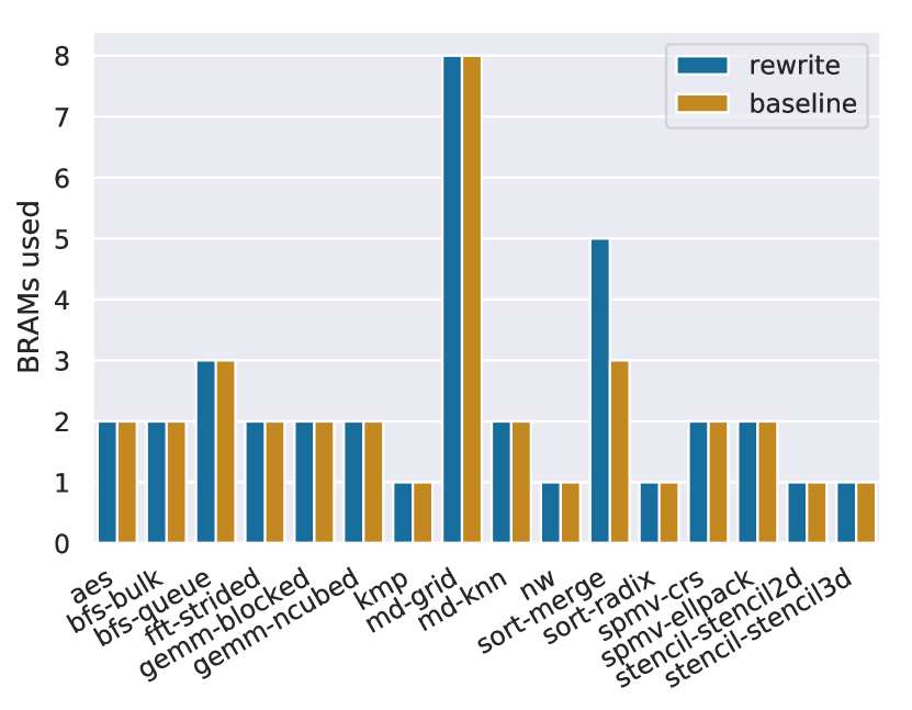
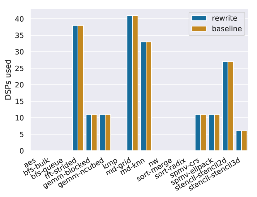
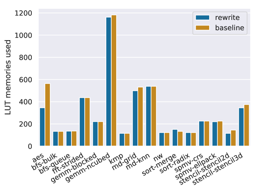
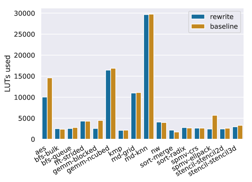
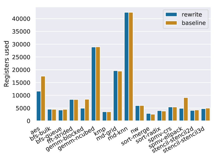
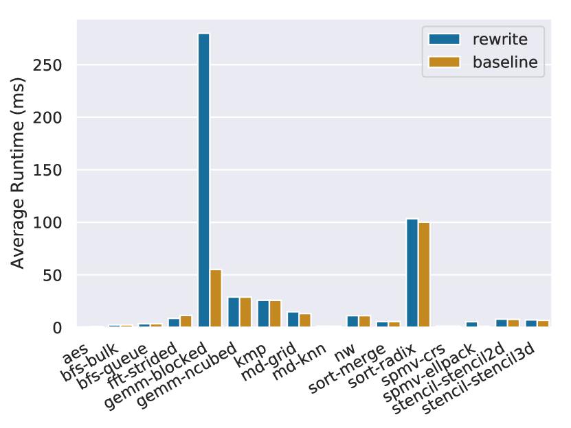
Appendix E Spatial Experiments

⬇

@spatial object GEMM_NCubed_16 extends SpatialApp {

type T = FixPt[TRUE,_16,_16]

def main(args: Array[String]): Unit = {

val (a_dram, b_data, c_data) = (DRAM[T](128,128), DRAM[T](128,128), DRAM[T](128,128))

// Generate random data for the input matrices.

val (a_data, b_data) = ((0::dim,0::dim){(i,j) => random[T](5)}, (0::dim,0::dim){(i,j) => random[T](5)})

// Set data in the input matrices.

setMem(a_dram, a_data)

setMem(b_dram, b_data)

// Accelerator kernel.

Accel {

val (a_sram, b_sram, c_sram) = (SRAM[T](dim,dim), SRAM[T](dim,dim), SRAM[T](dim,dim))

// Load data into memories.

a_sram.load(a_dram)

b_sram.load(b_dram)

// Computation loop.

Foreach(dim by 1) { i => Foreach(dim by 1) { j =>

// DSE parameter: Innermost loop parallelism. Try values from [1, 16].

val sum = Reduce(Reg[T](0))(dim by 1 par ::UNROLL::) { k => a_sram(i,k) * b_sram(k,j) }{_+_}

c_sram(i,j) = sum

}}

c_dram store c_sram

}

// Compute the expected value of the computation.

val c_gold = (0::dim,0::dim){(i,j) => Array.tabulate(dim){k => a_data(i,k) * b_data(k,j)}.reduce{_+_}}

// Check that the computed values are within some range of the expected value.

val c_result = getMatrix(c_dram)

val cksum = c_gold.zip(c_result){(a,b) => abs(a-b) < 0.5.to[T]}.reduce{_&&_}

// Fail if the computed value is different.

assert(cksum)

}

}

Figure 12. Kernel used to collect resource utilization number for the Spatial evaluation.

(a) Banking decision Spatial made given the unrolling factors.

(b) Resource usage normalized against no unrolling.

(c) Absolute DSP usage. Predictable points highlighted.

(d) Absolute REG usage. Predictable points highlighted.

(e) Absolute LUT usage. Predictable points highlighted.

(f) Absolute BRAM usage. Predictable points highlighted.

Figure 13. Resource utilization for gemm-ncubed design in Spatial on a Zynq-7000. Absolute resource utilization shows extreme variation between adjacent design points.

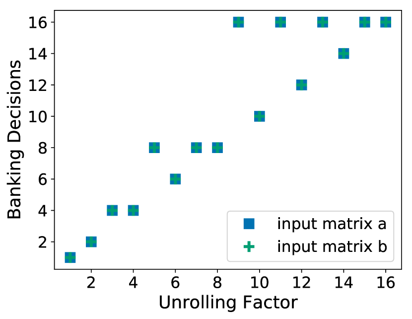
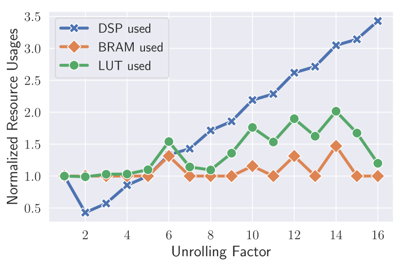
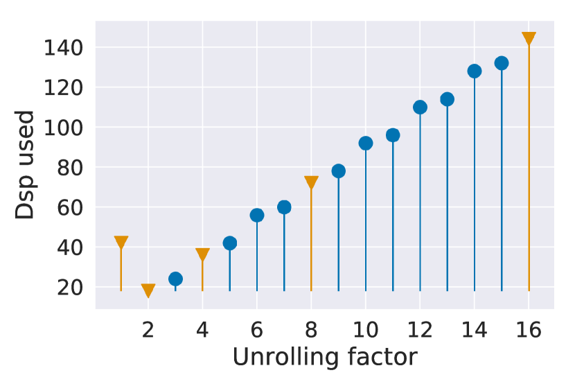
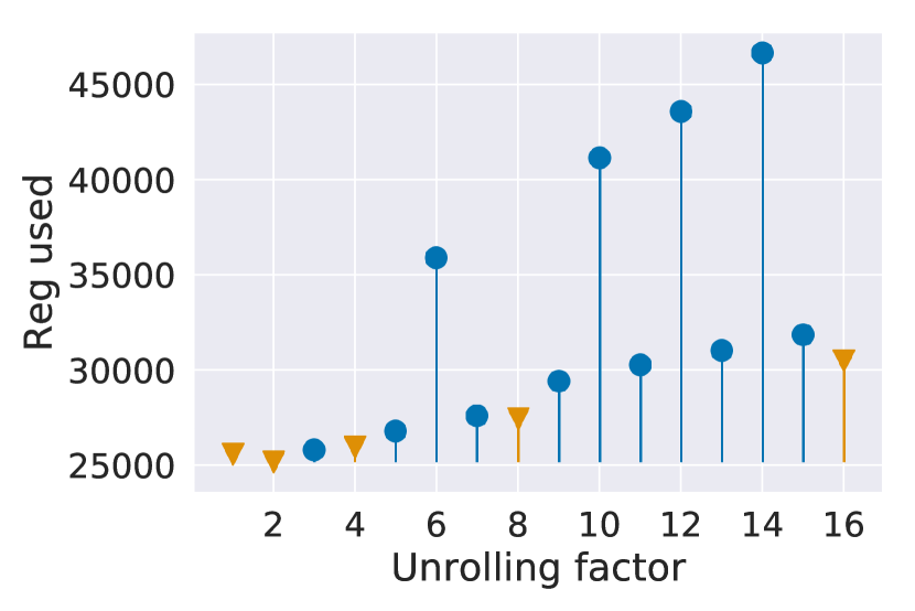
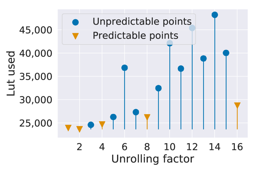
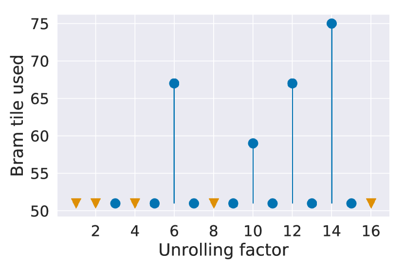
We perform a simple design sweep over a general matrix multiply kernel written in Spatial and vary the unrolling factor from $1$ to $16$.

We run the generated designs through a full synthesis flow by targeting Xilinx’s Zynq-7000 SoC (zynq). We extended the Spatial quick-start template to generate designs for the DSE comparison (dahlia-spatial). We were unable to get Spatial designs to pass through the AWS F1 based synthesis flow due to numerous issues (spatial-error-1; spatial-error-2; spatial-error-3).

Figure 13(a) shows the banking factors inferred by Spatial for a given unrolling factor. Figure 13(b) plots the resources usages normalized against the spatial design with no unrolling. When Spatial’s inferred banking decisions are not aligned with the unrolling factor, the resource usages abruptly increase.

We also plot the absolute LUT, DSP, REG and BRAM usage against unrolling factor in Figures 13(e), 13(c), 13(d) and 13(f). The designs use significantly fewer LUTs when the unrolling factor is a factor of the size of the memory. Furthermore, Spatial designs use up to $10\times$ more LUTs and $2\times$ more DSPs than the equivalent designs generated by Dahlia’s Vivado HLS backend.

Spatial uses automated design space exploration tools to find optimal parameters for the design. Dahlia’s type system can be used to eliminate unpredictable design points and drastically reduce the search spaces with such automated tools.