remarkRemark \headersConvexification Method for a 1D Wave EquationA. Smirnov, M. Klibanov, A. Sullivan and L. Nguyen
Convexification for an Inverse Problem
for a 1D Wave Equation with Experimental Data††thanks:
Submitted to the editors DATE.
\fundingThe workof AVS and MVK was supported
by US Army Research Laboratory and US Army Research Office grant W911NF-19-1-0044.
Abstract
The forward problem here is the Cauchy problem for a 1D hyperbolic PDE with a variable coefficient in the principal part of the operator. That coefficient is the spatially distributed dielectric constant. The inverse problem consists of the recovery of that dielectric constant from backscattering boundary measurements. The data depend on one variable, which is time. To address this problem, a new version of the convexification method is analytically developed. The theory guarantees the global convergence of this method. Numerical testing is conducted for both computationally simulated and experimental data. Experimental data, which are collected in the field, mimic the problem of the recovery of the spatially distributed dielectric constants of antipersonnel land mines and improvised explosive devices.
Key words: experimental data, 1D hyperbolic equation with a variable coefficient, coefficient inverse problem, convexification, globally convergent numerical method, Carleman estimate, numerical results
AMS Classification 35R30
1 Introduction
In this paper, we first develop a new globally convergent numerical method for a Coefficient Inverse Problem (CIP) for a 1D hyperbolic equation. This is a version of the so-called convexification method, which has been actively developed by the second coauthor and his coauthors for the past several years, see, e.g. [2, 17, 29, 18, 20, 22, 27, 26, 24, 36] for some samples of those publications. First, we test this method on computationally simulated data. Next, we test it on experimental time dependent data collected by the US Army Research Laboratory (ARL) using their forward looking radar [32]. These data were collected in the field which is a more difficult case than the collection in a laboratory. A significant challenge here is that targets were surrounded by clutter.
That radar was built to image and identify flash explosive-like targets, mainly antipersonnel land mines and improvised explosive devices. Those targets can be located both in air and under the ground. In the latter case, the burial depth does not exceed 10 centimeters. Currently ground penetrating radars rely only on the information about the energy of the backscattering signals. In our case, however, we computationally estimate dielectric constants of those targets. We hope that estimates of dielectric constants of explosive-like targets might serve in the future classification algorithms as an additional parameter to the currently used ones. The use of an additional parameter, in turn might decrease the current false alarm rate.
Although this research group has a number of publications where these experimental data are treated, in each of them either Laplace or Fourier transform of the experimental data with respect to the time is considered [16, 28, 24, 23, 30]. But since our data are actually time resolved ones, then we work here directly in the time domain.
Given a CIP, we call a numerical method for it globally convergent, if the theory rigorously guarantees that one can obtain at least one point in a sufficiently small neighborhood of the exact solution without an assumption that the starting point of iterations is located in this neighborhood. The global convergence issue is obviously important since it is very rare in applications when a good first approximation for the solution is available a priori.
Any CIP is both nonlinear and ill-posed. These factors cause the well known phenomenon of multiple local minima and ravines of conventional Tikhonov-like least squares functionals, see, e.g. [35] for a convincing example of this phenomenon. Conventional numerical methods for CIPs rely on the minimization of such functionals, see, e.g. [9] for some examples with a study of some experimental data in [15, 14].
Unlike conventional approaches, the concept of the convexification is designed with the goal to avoid local minima and ravines, see section 4.1 for a brief outline of the convexification. The first publications about this concept were in 1995 and 1997 [18, 20]. However, numerical studies were not conducted at that time since there were a number of theoretical issues which needed to be clarified to pave the way for numerical testing, although, see some numerical examples in the book [29]. Those issues were clarified more recently in the paper [2]. This publication has generated a number of papers with numerical studies. As some examples of those we mention [17, 22, 27, 26, 24, 23, 36]. In particular, in [26] the convexification is applied to a CIP with single measurement data for a 3D hyperbolic PDE.
To work with the experimental data of ARL in the time domain, one needs to have a numerical method for a CIP for a 1D hyperbolic PDE. However, the convexification for CIPs for the 1D hyperbolic PDEs was not developed until the very recent work [36]. Even though the CIP of the current paper is reduced to the same CIP as the one in [36] for the equation the method of this paper is significantly different from the one of [36]. Indeed, in [36] an integral differential equation with the Volterra-like integrals is obtained under the condition that the unknown coefficient Unlike this, in the current paper we replace those Volterra-like integrals with a non local condition. This allows us to avoid imposing the non-negativity condition on The latter, in turn enables us not to impose some quite restrictive extra conditions on the target unknown coefficient see (3) and (8).
We now refer to some other numerically implemented globally convergent numerical methods for CIPs for hyperbolic PDEs. First, this is the paper of De Hoop, Kepley and Oksanen [12] for a 3D hyperbolic CIP with Dirichlet-to-Neumann map data. Next, this is a series of works of Kabanikhin with coauthors who have computationally implemented the Gelfand-Levitan method [16, 17] for both 1D and 2D cases. We also mention here works of Baudouin, de Buhan, Ervedoza and Osses [3, 4], where a different version of the convexification for CIPs for hyperbolic PDEs in the D case is developed, also see more recent works of Boulakia, de Buhan and Schwindt [7] and Le and Nguyen [31], where the idea of [3] is developed further to apply to some nonlinear inverse problems for parabolic PDEs. The common property of these works and the above cited works on the convexification is that both substantially use Carleman estimates and the resulting numerical methods converge globally in both cases.
However, there is a significant difference between [3, 4] and the above cited publications on the convexification [17, 29, 18, 20, 22, 26, 24, 23, 36]. More precisely, [3, 4] work under an assumption of the Bukhgeim-Klibanov method [8]. This assumption is that one of initial conditions is not vanishing in the entire domain of interest. The original version of the convexification uses this assumption in [5, 27]. On the other hand, in publications [17, 29, 18, 20, 22, 26, 24, 23, 36], so as in this paper, either the initial condition, or a corresponding right hand side of a PDE is vanishing.
The convexification has significant roots in the idea of the paper [8] (1981), in which the tool of Carleman estimates was introduced in the field of CIPs for the first time. The original goal of [8] was limited to proofs of global uniqueness theorems for multidimensional CIPs. Therefore, the convexification can be regarded as an extension of the concept of [8] from the purely theoretical uniqueness topic to a more applied topic of globally convergent numerical methods for CIPs. Since 1981, many works of many authors have been devoted to a variety of applications of the method of [8] to proofs of uniqueness and stability results for many CIPs. Since the current paper is not a survey of these works, we now refer here only to the books [5, 6, 29] and the survey [19].
All functions below are real valued ones. In section 2, we formulate both forward and inverse problems. In section 3, we derive a quasilinear 1D hyperbolic PDE with a non local condition. In section 4, we introduce a weighted Tikhonov-like functional, which is the main subject of the convexification. In section 5, we formulate theorems about that functional, ensuring the global convergence of the resulting gradient projection method. Section 6 contains the proofs of theorems formulated in section 5. In section 7, we describe the algorithms, as well as accompanying procedures used to obtain the numerical results for both computationally simulated and experimental data.
2 Statements of Forward and Inverse Problems
Let be a number and the function has the following properties
| (1) | |||
| (2) |
Physically is the spatially distributed dielectric constant, where is the refractive index. In acoustics is the speed of sound. Let the number Consider the following Cauchy problem:
| (3) | |||
| (4) |
The problem of finding the function from conditions (3), (4) is our forward problem. Our interest is in the following inverse problem:
Coefficient Inverse Problem 1 (CIP1). Suppose
that the following two functions
are known:
| (5) |
Determine the function for assuming that the number is known.
We now introduce a change of variables in order to reduce the hyperbolic equation (3) to the wave-like equation with the unknown potential function and the constant principal part of the 1D hyperbolic operator. This is a well known change of variables, see, e.g. formulas (2.141)-(2.143) in section 7 of chapter 2 of the book of Romanov [34]. Thus, we introduce a new variable as
| (6) |
Physically, is the travel time needed for the wave to travel from the source to the point Denote
| (7) | |||
| (8) |
Then, using (3), (4) and (6)-(8), we obtain
| (9) | |||
| (10) |
where the number depends on . Using again (1), (2) and (5)-(8), we obtain
| (11) | |||
| (12) | |||
Existence and uniqueness of the solution of the forward problem (9)-(10) is well known. More precisely, it was proven in, e.g. section 3 of chapter 2 of [34], that
| (13) | |||
| (14) |
Equation (13) is a Volterra-like integral equation of the second kind. Hence, it can be solved via sequential iterations. The corresponding series converges absolutely in appropriate bounded subdomains of together with its derivatives up to the third order [34]. The existence of third derivatives of iterates is guaranteed by and (13). Thus,
| (15) |
If we would find the function then the function can be reconstructed via backward calculations, see section 7 for details. Therefore, we arrive at CIP2.
Coefficient Inverse Problem 2 (CIP2). Suppose that the number in (1) and the functions in (12) are known. Determine the coefficient in (9) for
Note that the number is unknown and should be determined when solving CIP2 and also (1) implies that However, we can estimate using (1), (2) as Hence, we fix a number such that
| (16) |
We use this number everywhere below. It was established in [34] that guarantees uniqueness of CIP2. Hence, we take below
| (17) |
Traditionally, classical absorbing boundary conditions of Engquist and Majda [13] are artificially imposed when working with the propagation of waves. In our case, however, Lemma 1 guarantees that the absorbing boundary condition is satisfied indeed at any two point and . We see in our computations that this condition is important, since it provides a better stability property.
Lemma 1 (absorbing boundary conditions). Let and be two arbitrary number. Then the solutions of problem (3), (4) and of problem (9), (10) satisfy the absorbing boundary condition at and i.e.
| (18) | ||||
| (19) | ||||
| (20) | ||||
| (21) |
We omit the proof of Lemma 1 since it mainly follows from Lemma 2.2 of [36]. Indeed, in the cases of (18) and (19) the proof of Lemma 1 is completely similar with the proof of Lemma 2.2 of [36]. In the cases of (20) and (21), in the proof of Lemma 2.2 of [36], one should take into account (7), (8) and (11), which can be done easily.
3 A Quasilinear PDE with a Non Local Term
Consider the rectangle
| (22) |
Here, is as in (17). Consider the function defined as:
| (23) |
Then, using (9) and (14), we obtain
| (24) |
and Hence,
| (25) |
Differentiate both sides of equation (24) with respect to , see (15) and denote
| (26) |
Then (5), (12), (14) and (23)-(26) lead to:
| (27) | |||
| (28) | |||
| (29) |
The condition follows from (16), Lemma 1 and (23). The problem (27)-(28) is a boundary value problem (BVP) for a 1D quasilinear hyperbolic equation (27) with overdetermined boundary conditions (28), an absent initial condition at and a non local term
4 Globally Strictly Convex Tikhonov-like Cost Functional
4.1 The main idea of the convexification
The first step of the convexification basically consists in obtaining an over-determined boundary value problem (BVP) for either a quasilinear integral differential equation with Volterra integrals in it [21, 22, 27, 36] or for a coupled system of elliptic PDEs [17, 26, 25, 24]. The common point of both is that neither of these PDEs contains the unknown coefficient. The latter reminds one the first step of the method of [8].
Next, to solve this BVP, a weighted Tikhonov-like functional is constructed, where is the parameter. The weight is the Carleman Weight Function (CWF). This is the function, which is involved as the weight in the Carleman estimate for the corresponding PDE operator. This functional is evaluated on a convex bounded set of the diameter where is an arbitrary but fixed number and is an appropriate Sobolev space. The central theorem then is that, for a proper choice of the parameter of the functional this functional is strictly convex on for all This eliminates the above mentioned phenomenon of multiple local minima. Next, results of [2] enable one to prove existence and uniqueness of the minimizer of on as well as the convergence of the gradient projection method to the exact solution if starting from an arbitrary point of the set Since the number is an arbitrary one, then this is the global convergence, see section 1. We also note that even though the theory requires the parameter to be sufficiently large, our extensive computational experience with the convexification, including the current paper (see section 7.1), tells us that provides quite accurate reconstructions [17, 22, 27, 26, 25, 24, 36].
4.2 The Tikhonov-like Cost Functional for BVP (27)-(28)
Since for the integration in (13) is carried out over the rectangle
| (31) |
The change of variables (23) transforms to the
following triangle
Hence, it follows from (30) that if we would find the function in the triangle (see Figure 1), then
we would find the function for . Here,
| (32) |


The CWF in this paper is the same as the one in [36],
| (33) |
where and are parameters independent on . Following (27), consider the quasilinear operator ,
| (34) |
Let be an arbitrary number. Consider the convex set of the diameter
| (35) |
where functions are defined in (29). Our Tikhonov-like cost functional functional is
| (36) |
where is the regularization parameter. The
reason why we use the space in the penalty
term of (36) is that in the proof of Theorem 2 (below), we require
as well as
| (37) |
Embedding theorem guarantees these. At the same time, we have established numerically that we can use the discrete analog of in the penalty term in our computations, see section 7. Here and below denotes different positive numbers depending only on the rectangle We concentrate below on the solution of the following minimization problem:
Minimization Problem. Find a minimizer of the
functional on the set
We introduce two functional spaces and
where the condition is introduced due to the last condition (28).
5 Convergence Analysis
In this section we formulate some theorems, which provide the convergence analysis of our method of solving the above Minimization Problem.
Theorem 1 (Carleman estimate). Let be the function defined in (33). Then there exists a number and another number depending only on listed parameters, such that for all functions and for all the following Carleman estimate is valid:
Let be the triangle defined in (32), where is the rectangle defined in (22). Choose an arbitrary number Define the triangle as
| (38) |
Let be a Hilbert space, be a convex set in and be a functional, which has the Frechét derivative at any point We remind that the following estimate guarantees the strict convexity of on the set
| (39) |
for all [33]. Here, the constant is independent on .
Theorem 2 (the central theorem: global strict convexity). For any pair and for any function the functional has the Frechét derivative Let be the number of Theorem 1 and let the number There exist a sufficiently large number and a number , both depending only on listed parameters, such that for all and for all
the functional is strictly convex on the set , i.e. (see (39))
Below and denote different numbers depending only on listed parameters.
Theorem 3. Let parameters be the same as in Theorem 2. Then there exists unique minimizer of the functional on the set Furthermore, the following inequality holds
We now want to estimate the accuracy of the reconstruction in the presence of noise in the data. Following one of the main concepts of the regularization theory, we assume is the existence of the exact solution of the CIP2 with the ideal noiseless data [5, 37]. Furthermore, we assume that conditions (11) hold for the function . Let be the corresponding function . We assume that where functions are the noiseless data in (28). It follows from (27) and (30) that
| (40) |
Let be the level of noise in the data. We assume that the number
| (41) |
is the noise level in the data. Suppose that there exist functions and
such that
| (42) |
Introduce functions and as
Let be an arbitrary number. Define
| (43) |
Using (41)-(43) and the triangle inequality, we obtain
| (44) | |||
| (45) |
We now consider a modification of the functional
| (46) |
Theorem 4. The functional has the Frechét derivative for every point and for all Denote where is the number of Theorem 2. For every and for every the functional is strictly convex on the ball i.e. (see (39)),
| (47) |
Furthermore, there exists unique minimizer of the functional on the set and the following inequality holds
| (48) |
Theorem 5 (accuracy estimate). Suppose that Denote
| (49) |
Let the number be so small that where is the number of Theorem 4. Let Let the the numbers and be such that
| (50) | |||
| (51) |
Let be the minimizer of the functional on the set the existence and uniqueness of which is guaranteed by Theorem 4. Denote
| (52) | |||
| (53) |
Then the following estimates are valid
| (54) | |||
| (55) |
To minimize the functional on the set via the gradient projection mehod, we first consider the orthogonal projection operator of the space on the closed ball Let be an arbitrary point and the number The sequence of the gradient projection method is [2]:
| (56) |
Theorem 6. Let be the number of Theorem 2 and let be the number of Theorem 4. Let the numbers be the same as one in Theorem 5. Let and let the numbers and be the same as in (50) and (51) respectively. Let be the minimizer of the functional on the set , the existence and uniqueness of which is guaranteed by Theorem 4. Let the function be the one defined in (52). Consider functions see (44) and (45). Also, let and be the coefficients which are found from the functions and via (30) and (53) respectively. Then there exists a number depending only on listed parameters such that for any there exists a number such that the following convergence rates are valid:
| (57) | |||
| (58) | |||
| (59) | |||
| (60) |
Remark 5.1.
Estimates (57)-(60) imply that the sequence in (56) generates the sequence of coefficients which converges globally to the function . Also, the sequence converges globally to the exact coefficient as long as the level of the noise in the data tends to zero. The global convergence property is due to the fact that the starting point of iterations (56) is an arbitrary point of the ball and the radius of this ball is an arbitrary number.
Remark 5.2.
6 Proofs of Theorems 2,5,6
In this section, where the rectangle is defined in (22).
6.1 Proof of Theorem 2
Consider two arbitrary functions . Let By (35), (43) and the triangle inequality,
| (61) |
As it was noticed in section 4, embedding theorem implies Also, (37) and (61) lead to:
| (62) |
First, we evaluate the expression
where the operator is defined in (34). Hence,
| (63) |
In the right hand side of (63), the first term is linear with respect to and other terms are nonlinear respect to . Let be the linear part of the right hand side of (63), i.e.
Thus,
| (64) |
By (34) and (62) Hence, the Cauchy-Schwarz inequality and (62) imply that the right hand side of (64) can be estimated from the below as:
It follows from (36) and (64) that
| (65) |
where denotes the scalar product in Define the functional
as
| (66) |
Then is a bounded linear functional. Next, it follows from (65) that
Hence, is the Frechét derivative of the functional at the point By the Riesz theorem, there exists unique element
Thus, we set Hence, using (6.1)-(66), we obtain
| (67) |
We now apply Carleman estimate of Theorem 1 to the right hand side of (67),
6.2 Proof of Theorem 5
| (71) |
| (72) |
Since functions and since by embedding theorem then (42) implies that Hence, using (36), (71) and (72), we obtain
| (73) |
By Theorem 4, for we consider the number Recall that numbers and are the same as in (50) and (51) respectively. Using (47), we obtain
| (74) |
Since and since by (48) then,
using (73), we estimate the first line of (74) from the
above as:
We now estimate from the below the second line of (74). It follows from (42), (5), (52) and the triangle inequality that
| (75) |
It follows from the Young’s inequality that for all Hence, (75) implies that
Similarly, using (42), (53) and the trace theorem, we obtain
| (76) |
Combining (74)-(76), we obtain
Or, equivalently,
| (77) |
Recall that and Since by (50) then in (77)
| (78) |
where is the number defined in (49). Thus, using (77) and (78), we obtain
| (79) | |||
| (80) |
Estimates (79) and (80) combined with (49) imply the target estimates (54) and (55) of this theorem.
6.3 Proof of Theorem 6
7 Numerical Implementation
In this section, we describe our numerical procedure to solve the Minimization Problem formulated in section 4.2. We work with the finite difference analog of the functional defined in (36). To do this, we use the uniform grid where . More precisely, for certain integers
| (81) |
In all numerical studies of this paper we take see (16). Therefore, by (22) we have as
We denote values of the function functions at the grid points of the domain by . Define the finite-difference analog of the operator in (34) at the point as
| (82) |
Following (30), denote
| (83) |
Thus, we define the finite difference analog of the functional as
| (84) |
Supplying the gradient of the functional via explicit formula significantly reduces computational time of the minimization procedure. The gradient of the functional is defined as a vector of partial derivatives with respect to the values of the function at the grid points
| (85) |
However the formula (85) is not an explicit one yet.
Hence, we use the formula , where denotes Kronecker symbol.
The following simplest example explains our idea of using Kronecker symbol on how to obtain explicit formulas of derivatives in (85)
Thus we obtain the following explicit formulas for the derivatives in (85)
| (86) |
where and .
The derivatives in (86) are defined only in the interior of the domain , defined in (81). In addition it is necessary to approximate the partial derivatives of on the boundary of this domain, using Taylor expansion of . This is because the function defined in (83) is updated on every iteration of the gradient descent method. Thus, for and we set
| (87) |
Thereafter for and
we define on the rest of the boundary, i.e. for and
, similarly to (84),(87).
Remark 7.1.
Note that the functional in (84) uses the Tikhonov regularization term in the norm instead of the required by the theory. We have established numerically that this is sufficient for computations.
7.1 Gradient descent method (GDM)
Even though Theorem 6 guarantees global convergence of the gradient projection method, we have numerically established that the simpler to implement gradient descent method (GDM) works well for our studies. The latter coincides with the conclusions of all above cited publications on the numerical studies of the convexification, e.g. see [2, 22, 27, 26, 24, 23]. We now apply the GDM to find the minimizer of functional (84). According to our theory, the initial guess for the GDM can be an arbitrary function . We choose the initial guess as the solution to the following problem, derived from (27)-(28) by setting and assuming for see (22). Thus,
which has the unique solution
| (88) |
where functions and are obtained from the pre-processed data (5), see Appendix for a more detailed explanation of the data simulation and pre-processing. In the case of the computationally simulated data the functions are obtained from the numerical solution of the Forward Problem (3)-(4) via the tridiagonal matrix algorithm [11].
Remark 7.2.
Other forms of the initial guess in a discrete analog of the set can also be chosen, see the section below. Such choices will not lead to significant different solutions, due to the global convergence of our numerical method, see Theorem 6 of section 5.
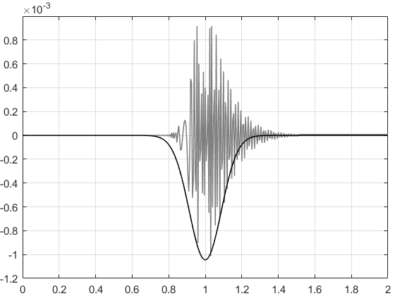
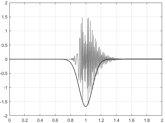
In all numerical tests of this paper we choose . In all further computations of inverse problems with simulated data we use the multiplicative random noise of the level i.e. . Since we use functions and we need to differentiate the noisy data , which we do by taking derivatives of the envelopes, see Figure 2. More detailed decription of data pre-processing and differentiation is given in Appendix.
The following values of parameters were used:
| (89) |
The parameters (89) were found by the trial and error procedure, and they work well for the numerical studies of this paper. We point out that even though our above theory requires large values of the parameter our numerical experience tells us that provides decent results. This is consistent with other numerical results on the convexification, where it was computationally established that works well numerically [2, 22, 27, 26, 24, 23]. The topic of optimal choices of parameters is outside of the scope of this paper. For brevity we use everywhere below notations for functions and variables in continuous setting, although we work with discrete setting as stated above.
Denote the result obtained on -th iteration of the GDM by . Using this function, we calculate the function via (30). After a sufficient number of iterations we come up with the computed coefficient . Thus we formulate Algorithm 1 for solving the Minimization Problem for functional on the set , i.e. in (35) is replaced with is replaced with the discrete analog of We use the discrete version of the space because the regularization term in uses the discrete form of the norm in this space.
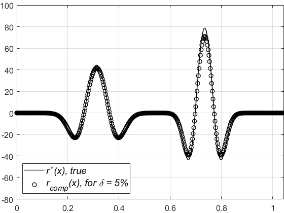
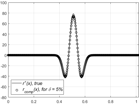
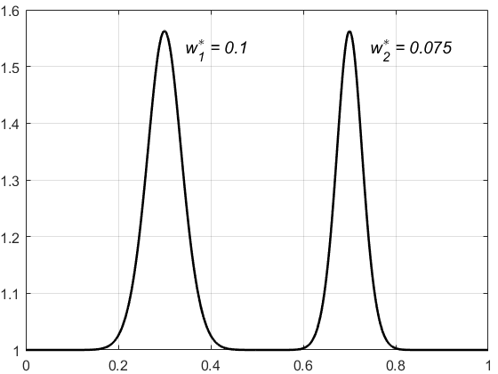
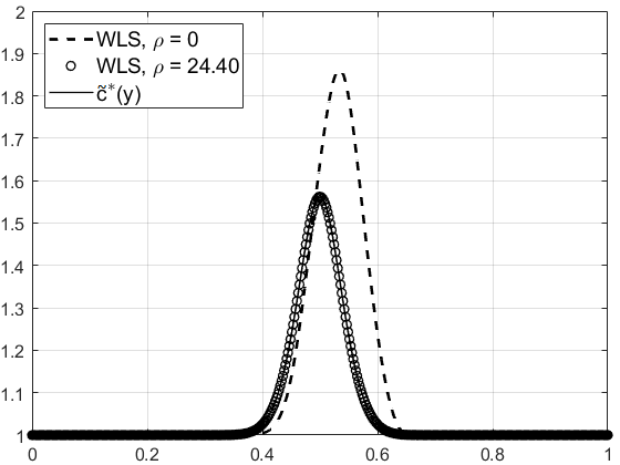
Thus, the numerical procedure described in Algorithm 1 delivers the numerical solution of the CIP2. We describe here two tests for the developed numerical algorithm. The calculated functions for both tests were interpolated with cubic splines on the finer grid with grid points. This interpolation is an important step for the reconstruction of the target functions , see section 6. The results of the reconstruction of the functions are depicted on Figure 3. The corresponding errors for the reconstructions are summarized in Table 1.
Test 1. The true function to be reconstructed as well as the simulated data were calculated from given by
| (90) |
where is full width at half maximum. The maximal value of the function is
max. For the first test we choose and , which corresponds to the maximal value of the dielectric constant of max, see Figure 3 (a) and solid line on Figure 4 (a).
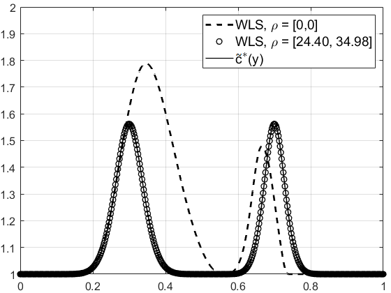
Test 2. The true function for the second test is calculated from given by the sum of two functions of the form (90), centered at and with and and , see Figure 3 (b) and solid line on 6 (a).
Table 1. Relative errors for the numerical solutions of the CIP2. Test 1. 0.0600 Test 2. 0.0900
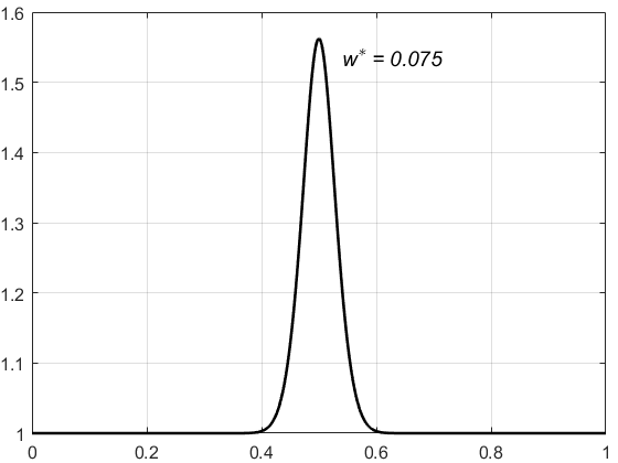
The horizontal axis depicts the values of .
7.2 Reconstruction of from the using weighted least-squares (WLS)
In this section we describe the second stage of the reconstruction procedure. More precisely, we show how to numerically reconstruct function from . Since and , then the upper estimate for the value of is max. However, we were only interested in the values of on the interval , therefore we enforce . Assume that the the values of the function are obtained via Algorithm 1 of section 7.1 on the interval . Relation between and is given by the quasilinear differential equation (8) coupled with (6).
Denote . Then, using the substitution we arrive at the following initial value problem for :
Given the function , find the function and satisfying
| (91) | |||
| (92) | |||
| (93) |
There are two significant difficulties associated with the numerical solution of problem (91)-(93). First, the dependence is unknown, whereas the right hand side of equation (91) is reconstructed by Algorithm 7.1 as the function of . Second, the problem (91)-(93) is overdetermined. We explain below how do we handle these two difficulties.
We have attempted to solve problem (91)-(93) via the Runge-Kutta method, on of the whole interval for a piecewise constant function without the condition
. Additionally, we assume here that . This allows us to recover and to compute via (93). However, we have observed numerically that this approach does not provide sufficiently accurate reconstructions due to the fact that the function attains both positive and negative values, see Figure 4 (a).
Hence, we formulate an alternative approach to solve problem (91)-(93). This approach requires the assumption . Note that this assumption is quite natural, because of (2).
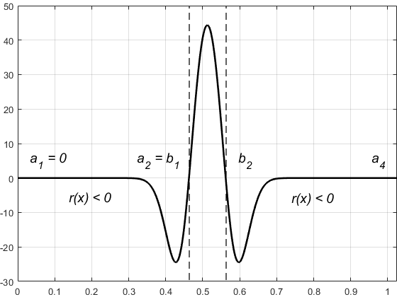
Assume that the function attains negative values on the intervals
and positive values on
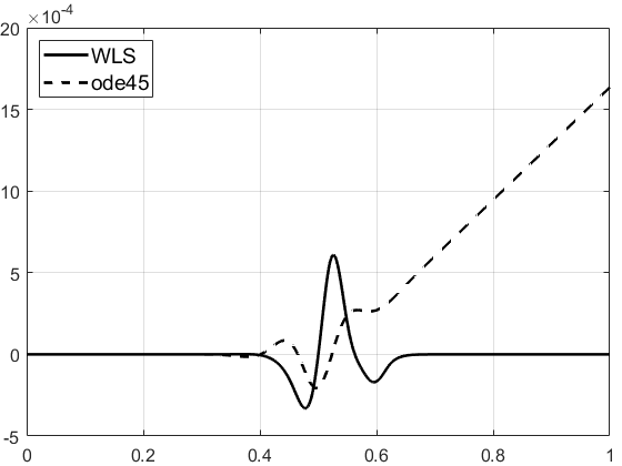
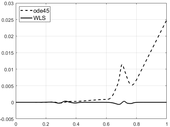
where numbers and are found approximately. To illustrate our idea, consider the simplest case of the function , depicted on Figure 4 (a). The corresponding function is defined in (90). We explain below how do we find the values and . We first, solve the problem (91)-(92) by the Runge-Kutta method on the subinterval without using the condition , as we have described earlier. Next, we solve problem (91)-(92) on the interval by WLS with a particular choice of the weight function. This approach provides a higher accuracy, compared with the Runge-Kutta method. The latter method results in a great deal of instability for , e.g. see Figure 5 (b) and Figure 6 (b). More precisely we minimize the following functional:
| (94) |
where is the parameter, which is similar to the parameter in the functionl . Numbers are found from the solution of the problem (91)-(93) on via the Runge-Kutta method, with in our particular case. Simultaneously with the minimizer we find the solution to the problem. See the results obtained via the described procedure on Figures 4, 6. The initial guess for the minimization of functional (94) is the cubic parabola , satisfying ,
at and at .
In the more general case, assuming that . Then the procedure is as follows:
-
a)
for each interval the Runge-Kutta method is applied,
-
b)
for each interval WLS is applied.
We have established numerically that this procedure is stable as long as not too many intervals are involved.
Remark 7.3.
As soon as is computed for , we solve (93) to find the dependence . Since the number is only an upper estimate for the interval of values of and since we know that , then we solve (93) by the Runge-Kutta method until either or . In our numerical experiments we observe that we always stop computation at . The latter allows us to tabulate the values of via . This is how Figures 5 and 6 are drawn.
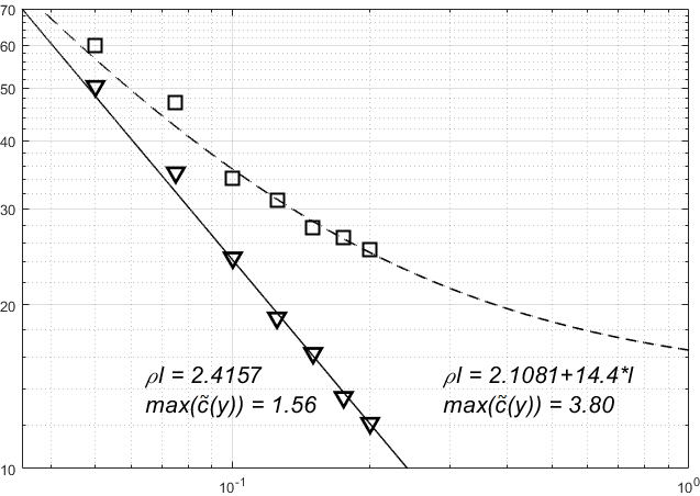
We can choose the parameter that leads to the lowest relative error in the reconstruction of . This parameter depends on the length of the interval . For a given pair an optimal value of the parameter is found numerically. The dependence of the optimal value on for two sets of functions is shown on Figure 4 (b). This technique can be used to reconstruct an arbitrary function , such that corresponding changes its sign on a finite number of intervals. In this paper, we use a simple model (90) to simulate the data. The optimal value of the parameter depends on the function . Since this paper considers only the functions of the form (90), then the values of the optimal parameters can be approximated using the values obtained from the simulated data for with a given and , see Figure 4 (b). We have found the optimal value for the data simulated for two types of functions of the form (90) with max and max. Next, we have found numerically that if max then the value of can be taken as
Combining the above steps, we arrive at Algorithm 2, which finds approximate values of on the whole interval .
Remark 7.4.
Remark 7.5.
Results depicted on Figure 6 demonstrate a significant accuracy improvement of the numerical reconstruction of by WLS method as compared with the conventional Runge-Kutta ”ode45” method of MATLAB.
Table 2. Values of dielectric constants, computed from experimental data. References containing intervals with correct values of dielectric constants are listed in the first column. Object max 1. Bush, see [10] 6.27 1 6.27 [3,20] 2. Wood stake, see [1] 3.21 1 3.21 [2,6] 3. Metal box (buried), see [1] 4.12 [10,30] 4. Metallic cylinder (buried), see [1] 5.39 [10,30] 5. Plastic cylinder (buried), see [1] 0.26 [0.5,1.5]
∗the value of the dielectric constant of the Object 5 is taken as = min.
Remark 7.6.
Note that the computed values of are close to the ones of [30], presented in Table 1 of section 8.
7.3 Numerical tests on experimental data
The experimental data were collected by A. Sullivan and L. Nguyen for five (5) objects. First two objects, bush and wood stake, were above the ground. The three buried objects were metallic box, plastic cylinder and metal cylinder. The data for each object contain 80 temporal samples with the time step , which corresponds to imaged distance from to meters. We measure the function . As to the function , we calculate it using and the absorbing boundary condition (21) of Lemma 1 for . The exact locations of targets were not of an interest to us since their horizontal coordinates were delivered quite accurately by GPS. For a more detailed description of the data acquisition scheme see section 7 of [30].
The dielectric constants were not measured when the data were collected. However, it was known that the burial depth of every underground target was a few centimeters. Additionally, we knew which targets were located above the ground and which ones were buried in the ground. Thus, we have computed the values of dielectric constants and compared with those listed in other references. The background for Objects 3-5, was dry sand, where dielectric constant belongs to [3,5], see [1]. Note that tables usually contain ranges of values of dielectric constants rather than their exact values [1]. Thus, the problem of the determination of the material from the experimental data becomes a problem to find the interval for the values of dielectric constant of the studied object and a further comparison with the known range of values.
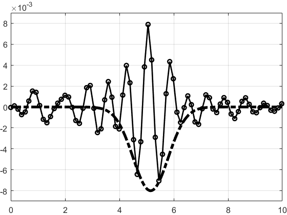
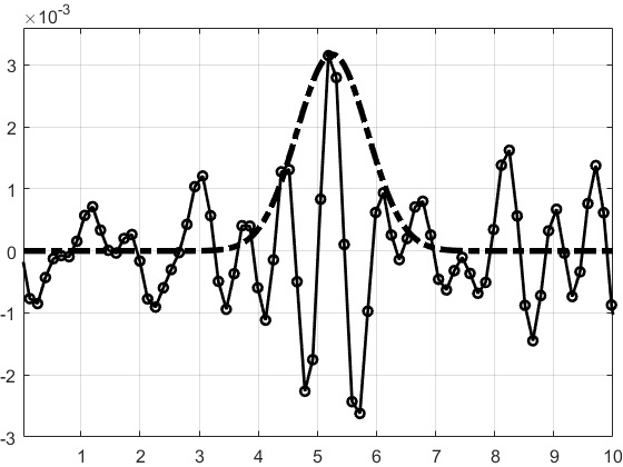
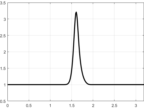
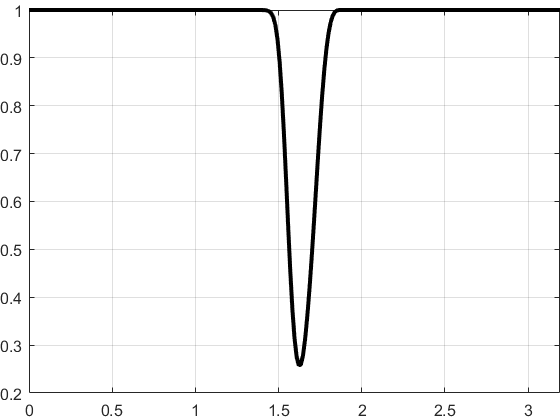
We also note that the data are 1D, whereas the objects are 3D. Thus, the images obtained here (see Figure 7 (c),(d)) can only be considered an approximate models of the real objects. We still apply the technique of section 7.3 of [30] for determining of whether the positive or negative values of the data should be used for the envelope for the buried objects, see Figures 7 (a),(b). Figures 7 (a),(b) depicts the data collected for two out of five objects. The data were scaled as in [30], we have multiplied the data by the scaling factor .
Since our method works on the domain different from the one for which the experimental data were collected, we scale the real time in nanoseconds as on the interval and use the notation for the scaled time onward. For Figures 7 (a),(b) the time was scaled back to the real time. We apply Algorithm 1 to reconstruct the function for each object. Next, Algorithm 2 is applied to find the corresponding dielectric constants. The estimated values of dielectric constants are listed in the Table 2. is the value of the dielectric constant of the background (air for Objects 1-2, dry sand for Objects 3-5). = max is the estimated dielectric constant of the Object. On the other hand, if the value of the dielectric constant of the Object is less that the one of the background, e.g. Object 5 (plastic cylinder), then = min is taken as the dielectric constant of the Object. is the value of the dielectric constant found in the corresponding reference; those references are listed in the first column of Table 2.
Conclusions. It is clear from columns 4, 5 of Table 2 that computed dielectric constants belong to appropriate intervals, furthermore we notice that our computed dielectric constants are close to the ones of Table 1 of [30].
Appendix A Data simulation and pre-processing
Let the function be given. Consider the domain and a with , . Then, to simulate the data for the inverse problem CIP2, we solve the following initial value problem problem
which is an analog of problem (3)-(4) supplemented with the absorbing boundary condition. In addition, for our numerical studies we replaced the initial condition with the gaussian exp. The numerical solution of the problem stated above via finite differences delivers the approximate function , which is used to compute functions , .
By (29), the data for the inverse problem, i.e. , contain first and second derivatives of the functions , which can not be retrieved numerically due to high oscillations in the values of the considered functions. Thus, we use their envelopes to approximate the functions . First, we filter the data by taking only negative values and truncating to zero the values of the functions which are less than max and max respectively. This is true for objects having the dielectric constants greater than the one of the background. On the other hand, for the above case of the plastic cylinder, buried in the ground we use the positive values of the functions with the same truncation rule, see section 7.3 of [30]. Next, we approximate so truncated functions with the envelopes of the following forms:
| (95) |
where the sign is chosen according to the previous arguments. The parameters are found using weighted least-squares curve fit (”fit” function) of the Curve Fitting Toolbox of MATLAB. Samples of approximations (95) are depicted on Figure 2.
Then, based on (29), we set and , where the derivatives of are found explicitly.
References
- [1] Clipper controls inc. (n.d.) dielectric constants of various materials., http://www.clippercontrols.com/pages/Dielectric-Constant-Values.html.
- [2] A. B. Bakushinskii, M. V. Klibanov, and N. A. Koshev, Carleman weight functions for a globally convergent numerical method for ill-posed Cauchy problems for some quasilinear pdes, Nonlinear Anal. Real World Appl., 34 (2017), pp. 201–224.
- [3] L. Baudouin, M. De Buhan, and S. Ervedoza, Convergent algorithm based on carleman estimates for the recovery of a potential in the wave equation, SIAM Journal on Numerical Analysis, 55 (2017), pp. 1578–1613.
- [4] L. Baudouin, M. de Buhan, S. Ervedoza, and A. Osses, Carleman-based reconstruction algorithm for the waves, (2020), https://hal.archives-ouvertes.fr/hal-02458787.
- [5] L. Beilina and M. V. Klibanov, Approximate Global Convergence and Adaptivity for Coefficient Inverse Problems, Springer, New York, 2012.
- [6] M. Bellassoued and M. Yamamoto, Carleman Estimates and Applications to Inverse Problems for Hyperbolic Systems, Springer, Japan, 2017.
- [7] M. Boulakia, M. de Buhan, and E. Schwindt, Numerical reconstruction based on carleman estimates of a source term in a reaction-diffusion equation., (2019), https://hal.archives-ouvertes.fr/hal-02185889.
- [8] A. L. Bukhgeim and M. V. Klibanov, Uniqueness in the large of a class of multidimensional inverse problems, Soviet Math. Doklady, 17 (1981), pp. 244–247.
- [9] G. Chavent, Nonlinear least squares for inverse problems: theoretical foundations and step-by-step guide for applications, Springer Science & Business Media, 2010.
- [10] H. Chuah, K. Lee, and T. Lau, Dielectric constants of rubber and oil palm leaf samples at x-band, IEEE transactions on geoscience and remote sensing, 33 (1995), pp. 221–223.
- [11] S. D. Conte and C. De Boor, Elementary numerical analysis: an algorithmic approach, SIAM, 2017.
- [12] M. V. de Hoop, P. Kepley, and L. Oksanen, Recovery of a smooth metric via wave field and coordinate transformation reconstruction, SIAM Journal on Applied Mathematics, 78 (2018), pp. 1931–1953.
- [13] B. Engquist and A. Majda, Absorbing boundary conditions for numerical simulation of waves, Proceedings of the National Academy of Sciences, 74 (1977), pp. 1765–1766.
- [14] A. Goncharsky, S. Romanov, and S. Seryozhnikov, Low-frequency ultrasonic tomography: mathematical methods and experimental results, Moscow University Physics Bulletin, 74 (2019), pp. 43–51.
- [15] A. V. Goncharsky and S. Y. Romanov, A method of solving the coefficient inverse problems of wave tomography, Computers & Mathematics with Applications, 77 (2019), pp. 967–980.
- [16] A. L. Karchevsky, M. V. Klibanov, L. Nguyen, N. Pantong, and A. Sullivan, The krein method and the globally convergent method for experimental data, Applied Numerical Mathematics, 74 (2013), pp. 111–127.
- [17] V. A. Khoa, M. V. Klibanov, and L. H. Nguyen, Convexification for a 3d inverse scattering problem with the moving point source, arXiv preprint arXiv:1911.10289, (2019).
- [18] M. V. Klibanov, Global convexity in a three-dimensional inverse acoustic problem, SIAM J. Math. Anal., 28 (1997), pp. 1371–1388.
- [19] M. V. Klibanov, Carleman estimates for global uniqueness, stability and numerical methods for coefficient inverse problems, J. Inverse and Ill-Posed Problems, 21 (2013), pp. 477–560.
- [20] M. V. Klibanov and O. V. Ioussoupova, Uniform strict convexity of a cost functional for three-dimensional inverse scattering problem, SIAM Journal on Mathematical Analysis, 26 (1995), pp. 147–179.
- [21] M. V. Klibanov and V. G. Kamburg, Globally strictly convex cost functional for an inverse parabolic problem, Mathematical Methods in the Applied Sciences, 39 (2016), pp. 930–940.
- [22] M. V. Klibanov, A. E. Kolesov, and D.-L. Nguyen, Convexification method for an inverse scattering problem and its performance for experimental backscatter data for buried targets, SIAM Journal on Imaging Sciences, 12 (2019), pp. 576–603.
- [23] M. V. Klibanov, A. E. Kolesov, L. Nguyen, and A. Sullivan, Globally strictly convex cost functional for a 1-d inverse medium scattering problem with experimental data, SIAM Journal on Applied Mathematics, 77 (2017), pp. 1733–1755.
- [24] M. V. Klibanov, A. E. Kolesov, A. Sullivan, and L. Nguyen, A new version of the convexification method for a 1d coefficient inverse problem with experimental data, Inverse Problems, 34 (2018), p. 115014.
- [25] M. V. Klibanov, J. Li, and W. Zhang, Electrical impedance tomography with restricted dirichlet-to-neumann map data, arXiv preprint arXiv:1803.11193, (2018).
- [26] M. V. Klibanov, J. Li, and W. Zhang, Convexification for the inversion of a time dependent wave front in a heterogeneous medium, SIAM Journal on Applied Mathematics, 79 (2019), pp. 1722–1747.
- [27] M. V. Klibanov, J. Li, and W. Zhang, Convexification for an inverse parabolic problem, arXiv preprint arXiv:2001.01880, (2020).
- [28] M. V. Klibanov, L. H. Nguyen, A. Sullivan, and L. Nguyen, A globally convergent numerical method for a 1-d inverse medium problem with experimental data, Inverse Problems and Imaging, 10 (2016), pp. 1057–1085.
- [29] M. V. Klibanov and A. Timonov, Carleman Estimates for Coefficient Inverse Problems and Numerical Applications, Inverse and Ill-Posed Problems Series, VSP, Utrecht, 2004.
- [30] A. Kuzhuget, L. Beilina, M. Klibanov, A. Sullivan, L. Nguyen, and M. A. Fiddy, Blind backscattering experimental data collected in the field and an approximately globally convergent inverse algorithm, Inverse Problems, 28 (2012), p. 095007.
- [31] T. T. Le and L. H. Nguyen, A convergent numerical method to recover the initial condition of nonlinear parabolic equations from lateral cauchy data, arXiv preprint arXiv:1910.05584, (2019).
- [32] L. Nguyen, D. Wong, M. Ressler, F. Koenig, B. Stanton, G. Smith, J. Sichina, and K. Kappra, Obstacle avoidance and concealed target detection using the army research lab ultra-wideband synchronous impulse reconstruction (uwb sire) forward imaging radar, in Detection and Remediation Technologies for Mines and Minelike Targets XII, vol. 6553, International Society for Optics and Photonics, 2007, p. 65530H.
- [33] B. T. Polyak, Introduction to optimization. optimization software, Inc., Publications Division, New York, 1 (1987).
- [34] V. G. Romanov, Inverse problems of mathematical physics, Walter de Gruyter GmbH & Co KG, 2018.
- [35] J. A. Scales, M. L. Smith, and T. L. Fischer, Global optimization methods for multimodal inverse problems, J. Computational Physics, 103 (1992), pp. 258–268.
- [36] A. V. Smirnov, M. V. Klibanov, and L. H. Nguyen, Convexification for a 1d hyperbolic coefficient inverse problem with single measurement data, arXiv preprint arXiv:2002.01074, (2020).
- [37] A. N. Tikhonov, A. Goncharsky, V. Stepanov, and A. G. Yagola, Numerical methods for the solution of ill-posed problems, vol. 328, Springer Science & Business Media, 2013.
