Exemplar VAE:   Linking Generative Models,
Nearest Neighbor Retrieval, and Data Augmentation

Abstract

We introduce Exemplar VAEs, a family of generative models that bridge the gap between parametric and non-parametric, exemplar based generative models. Exemplar VAE is a variant of VAE with a non-parametric prior in the latent space based on a Parzen window estimator. To sample from it, one first draws a random exemplar from a training set, then stochastically transforms that exemplar into a latent code and a new observation. We propose retrieval augmented training (RAT) as a way to speed up Exemplar VAE training by using approximate nearest neighbor search in the latent space to define a lower bound on log marginal likelihood. To enhance generalization, model parameters are learned using exemplar leave-one-out and subsampling. Experiments demonstrate the effectiveness of Exemplar VAEs on density estimation and representation learning. Importantly, generative data augmentation using Exemplar VAEs on permutation invariant MNIST and Fashion MNIST reduces classification error from 1.17% to 0.69% and from 8.56% to 8.16%. Code is available at https://github.com/sajadn/Exemplar-VAE.

1 Introduction

Non-parametric, exemplar based methods use large, diverse sets of exemplars, and relatively simple learning algorithms such as Parzen window estimation [46] and CRFs [35], to deliver impressive results on image generation (e.g., texture synthesis [16], image super resolution [17], and inpaiting [10, 26]). These approaches generate new images by randomly selecting an exemplar from an existing dataset, and modifying it to form a new observation. Sample quality of such models improves as dataset size increases, and additional training data can be incorporated easily without further optimization. However, exemplar based methods require a distance metric to define neighborhood structures, and metric learning in high dimensional spaces is a challenge in itself [29, 59].

Conversely, conventional parametric generative models based on deep neural nets enable learning complex distributions (e.g., [45, 49]). One can use standard generative frameworks [14, 15, 19, 33, 51] to optimize a decoder network to convert noise samples drawn from a factored Gaussian distribution into real images. When training is complete, one would discard the training dataset and generate new samples using the decoder network alone. Hence, the burden of generative modeling rests entirely on the model parameters, and additional data cannot be incorporated without training.

This paper combines the advantages of exemplar based and parametric methods using amortized variational inference, yielding a new generative model called Exemplar VAE. It can be viewed as a variant of Variational Autoencoder (VAE) [33, 51] with a non-parametric Gaussian mixture (Parzen window) prior on latent codes.

To sample from the Exemplar VAE, one first draws a random exemplar from a training set, then stochastically transforms it into a latent code. A decoder than transforms the latent code into a new observation. Replacing the conventional Gaussian prior into a non-parameteric Parzen window improves the representation quality of VAEs as measured by kNN classification, presumably because a Gaussian mixture prior with many components captures the manifold of images and their attributes better. Exemplar VAE also improves density estimation on MNIST, Fashion MNIST, Omniglot, and CelebA, while enabling controlled generation of images guided by exemplars.

We are inspired by recent work on generative models augmented with external memory (e.g., [24, 38, 57, 31, 4]), but unlike most existing work, we do not rely on pre-specified distance metrics to define neighborhood structures. Instead, we simultaneously learn an autoencoder, a latent space, and a distance metric by maximizing log-likelihood lower bounds. We make critical technical contributions to make Exemplar VAEs scalable to large datasets, and enhance their generalization.

The main contributions of this paper are summarized as follows:

1. We introduce Exemplar VAE along with critical regularizers that combat overfitting;

2. We propose retrieval augmented training (RAT), using approximate nearest neighbor search in the latent space, to speed up training based on a novel log-likelihood lower bound;

3. Experimental results demonstrate that Exemplar VAEs consistently outperform VAEs with a Guassian prior or VampPrior [57] on density estimation and representation learning;

4. We demonstrate the effectiveness of generative data augmentation with Exemplar VAEs for supervised learning, reducing classification error of permutation invariant MNIST and Fashion MNIST significantly, from $1.17\%$ to $0.69\%$ and from 8.56% to 8.16% respectively.

2 Exemplar based Generative Models

By way of background, an exemplar based generative model is defined in terms of a dataset of $N$ exemplars, $X\equiv\{\bm{\mathbf{x}}_{n}\}_{n=1}^{N}$, and a parametric transition distribution, $T_{\theta}(\bm{\mathbf{x}}\mid\bm{\mathbf{x}}^{\prime})$, which stochastically transforms an exemplar $\bm{\mathbf{x}}^{\prime}$ into a new observation $\bm{\mathbf{x}}$. The log density of a data point $\bm{\mathbf{x}}$ under an exemplar based generative model $\{X,T_{\theta}\}$ can be expressed as

$$\log p(\bm{\mathbf{x}}\mid X,\theta)~{}=~{}\log\sum\nolimits_{n=1}^{N}\frac{1}{N}T_{\theta}(\bm{\mathbf{x}}\mid\bm{\mathbf{x}}_{n})~{},$$ (1)

where we assume the prior probability of selecting each exemplar is uniform. Suitable transition distributions should place considerable probability mass on the reconstruction of an exemplar from itself, i.e., $T_{\theta}(\bm{\mathbf{x}}\mid\bm{\mathbf{x}})$ should be large for all $\bm{\mathbf{x}}$. Further, an ideal transition distribution should be able to model the conditional dependencies between different dimensions of $\bm{\mathbf{x}}$ given $\bm{\mathbf{x}}^{\prime}$, since the dependence of $\bm{\mathbf{x}}$ on $\bm{\mathbf{x}}^{\prime}$ is often insufficient to make dimensions of $\bm{\mathbf{x}}$ conditionally independent.

One can view the Parzen window or Kernel Density estimator [46], as a simple type of exemplar based generative model in which the transition distribution is defined in terms of a prespecified kernel function and its meta-parameters. With a Gaussian kernel, a Parzen window estimator takes the form

$$\log p(\bm{\mathbf{x}}\mid X,\sigma^{2})~{}=~{}-\log C-\log N+\log\sum\nolimits_{n=1}^{N}\exp\frac{-\lVert\bm{\mathbf{x}}-\bm{\mathbf{x}}_{n}\rVert^{2}}{2\sigma^{2}}~{},$$ (2)

where $\log C=d_{x}\log(\sqrt{2\pi}\sigma)$ is the log normalizing constant of an isotropic Gaussian in $d_{x}$ dimensions. The non-parametric nature of Parzen window estimators enables one to exploit extremely large heterogeneous datasets of exemplars for density estimation. That said, simple Parzen window estimation typically underperforms parametric density estimation, especially in high dimensional spaces, due to the inflexibility of typical transition distributions, e.g., when $T(\bm{\mathbf{x}}\mid\bm{\mathbf{x}}^{\prime})=\mathcal{N}(\bm{\mathbf{x}}\mid\bm{\mathbf{x}}^{\prime},\sigma^{2}I)$.

This work aims to adopt desirable properties of non-parametric exemplar based models to help scale parametric models to large heterogeneous datasets and representation learning. In effect, we learn a latent representation of the data for which a Parzen window estimator is an effective prior.

3 Exemplar Variational Autoencoders

The generative process of an Exemplar VAE is summarized in three steps:

1. Sample $n\!\sim\!\mathrm{Uniform}(1,N)$ to obtain a random exemplar $\bm{\mathbf{x}}_{n}$ from the training set, $X\equiv\{\bm{\mathbf{x}}_{n}\}_{n=1}^{N}$.

2. Sample $\bm{\mathbf{z}}\!\sim\!r_{\phi}(\cdot\mid\bm{\mathbf{x}}_{n})$ using an exemplar based prior, $r_{\phi}$, to transform an exemplar $\bm{\mathbf{x}}_{n}$ into a distribution over latent codes, from which $\bm{\mathbf{z}}$ is drawn.

3. Sample $\bm{\mathbf{x}}\!\sim\!p_{\theta}(\cdot\mid\bm{\mathbf{z}})$ using a decoder to transform $\bm{\mathbf{z}}$ into a distribution over observations, from which $\bm{\mathbf{x}}$ is drawn.

Accordingly, the Exemplar VAE can be interpreted as a variant of exemplar based generative models in (1) with a parametric transition function defined in terms of a latent variable $\bm{\mathbf{z}}$, i.e.,

$$T_{\phi,\theta}(\bm{\mathbf{x}}\mid\bm{\mathbf{x}}^{\prime})~{}=~{}\int_{z}r_{\phi}(\bm{\mathbf{z}}\mid\bm{\mathbf{x}}^{\prime})\,p_{\theta}(\bm{\mathbf{x}}\mid\bm{\mathbf{z}})\,d\bm{\mathbf{z}}~{}.$$ (3)

This model assumes that, conditioned on $\bm{\mathbf{z}}$, an observation $\bm{\mathbf{x}}$ is independent from an exemplar $\bm{\mathbf{x}}^{\prime}$. This conditional independence simplifies the formulation, enables efficient optimization, and encourages a useful latent representation.

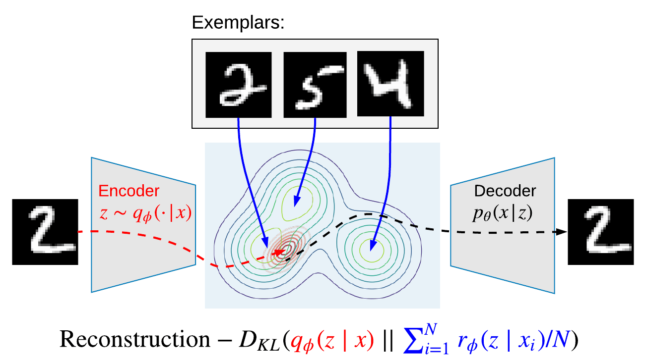
Figure 1: Exemplar VAE is a type of VAE with a non-parametric mixture prior in the latent space. Here, only $3$ exemplars are shown, but the set of exemplars often includes thousands of data points from the training dataset. The objective function is similar to a standard VAE with the exception that the KL term measures the disparity between the variational posterior $q_{\phi}(\bm{\mathbf{z}}\!\mid\!\bm{\mathbf{x}})$ and a mixture of exemplar based priors $\sum_{n=1}^{N}r_{\phi}(\bm{\mathbf{z}}\mid\bm{\mathbf{x}}_{n})/N$.

By marginalizing over the exemplar index $n$ and the latent variable $\bm{\mathbf{z}}$, one can derive an evidence lower bound (ELBO) [3, 30] on log marginal likelihood for a data point $\bm{\mathbf{x}}$ as follows (derivation in section F of supplementary materials):

$$\log p(\bm{\mathbf{x}};X,\theta,\phi) ~{}=~{}\log\sum_{n=1}^{N}\frac{1}{N}T_{\phi,\theta}(\bm{\mathbf{x}}\mid\bm{\mathbf{x}}_{n})~{}=~{}\log\sum_{n=1}^{N}\frac{1}{N}\int_{z}{r_{\phi}(\bm{\mathbf{z}}\mid\bm{\mathbf{x}}_{n})\,p_{\theta}(\bm{\mathbf{x}}\mid\bm{\mathbf{z}})}\,d\bm{\mathbf{z}}$$ (4)

$$~{}\geq~{}\underbrace{\mathop{\mathbb{E}}_{q_{\phi}(\bm{\mathbf{z}}\mid\bm{\mathbf{x}})}\!\!\!\log p_{\theta}(\bm{\mathbf{x}}\!\mid\!\bm{\mathbf{z}})}_{\mathrm{reconstruction}}~{}-\,\underbrace{\mathop{\mathbb{E}}_{q_{\phi}(\bm{\mathbf{z}}\mid\bm{\mathbf{x}})}\log\frac{q_{\phi}(\bm{\mathbf{z}}\mid\bm{\mathbf{x}})}{\sum\nolimits_{n=1}^{N}r_{\phi}(\bm{\mathbf{z}}\mid\bm{\mathbf{x}}_{n})/N}}_{\mathrm{KL~{}term}}$$

$$~{}=~{}O(\theta,\phi;\bm{\mathbf{x}},X).$$ (5)

We use (5) as the Exemplar VAE objective to optimize parameters $\theta$ and $\phi$. Note that $O(\theta,\phi;\bm{\mathbf{x}},X)$ is similar to the ELBO for a standard VAE, the difference being the definition of the prior $p(\bm{\mathbf{z}})$ in the KL term. The impact of exemplars on the learning objective can be summarized in the form of a mixture model prior in the latent space, with one mixture component per exemplar, i.e., $p\left(\bm{\mathbf{z}}\!\mid\!X\right)=\sum\nolimits_{n}\!r_{\phi}(\bm{\mathbf{z}}\mid\bm{\mathbf{x}}_{n})/N$. Fig. 1 illustrates the training procedure and objective function for Exemplar VAE.

A VAE with a Gaussian prior uses an encoder during training to define a variational bound [33]. Once training is finished, new observations are generated using the decoder network alone. To sample from an Exemplar VAE, we need the decoder and access to a set of exemplars and the exemplar based prior $r_{\phi}$. Importantly, given the non-parametric nature of Exemplar VAEs, one can train this model with one set of exemplars and perform generation with another, potentially much larger set.

As depicted in Figure 1, the Exemplar VAE employs two encoder networks, i.e., ${q}_{\phi}(\bm{\mathbf{z}}\!\mid\!\bm{\mathbf{x}})$ as the variational posterior, and $r_{\phi}(\bm{\mathbf{z}}\!\mid\!\bm{\mathbf{x}}_{n})$ for mapping an exemplar $\bm{\mathbf{x}}_{n}$ to the latent space for the exemplar based prior. We adopt Gaussian distributions for both ${q}_{\phi}$ and $r_{\phi}$. To ensure that $T(\bm{\mathbf{x}}\mid\bm{\mathbf{x}})$ is large, we share the means of ${q}_{\phi}$ and $r_{\phi}$. This is also inspired by the VampPrior [57] and discussions of the aggregated variational posterior as a prior [42, 28]. Accordingly, we define

$${q}_{\phi}(\bm{\mathbf{z}}\mid\bm{\mathbf{x}}) ~{}=~{}\mathcal{N}(\bm{\mathbf{z}}\mid\bm{\mu}_{\phi}(\bm{\mathbf{x}})\,,~{}\Lambda_{\phi}(\bm{\mathbf{x}})),$$ (6)

$$r_{\phi}(\bm{\mathbf{z}}\mid\bm{\mathbf{x}}_{n}) ~{}=~{}\mathcal{N}(\bm{\mathbf{z}}\mid\bm{\mu}_{\phi}(\bm{\mathbf{x}}_{n})\,,~{}\sigma^{2}I)~{}.$$ (7)

The two encoders use the same parametric mean function $\bm{\mu}_{\phi}$, but they differ in their covariance functions. The variational posterior uses a data dependent diagonal covariance matrix ${\Lambda}_{\phi}$, while the exemplar based prior uses an isotropic Gaussian (per exemplar), with a shared, scalar parameter $\sigma^{2}$. Accordingly, $\log p\left(\bm{\mathbf{z}}\!\mid\!X\right)$, the log of the aggregated exemplar based prior is given by

$$\log p\left(\bm{\mathbf{z}}\!\mid\!X\right)~{}=~{}-\log C^{\prime}-\log N+\log\sum\nolimits_{j=1}^{N}\exp\frac{-\lVert\bm{\mathbf{z}}-\bm{\mu}_{\phi}(\bm{\mathbf{x}}_{j})\rVert^{2}}{2\sigma^{2}}~{},$$ (8)

where $\log C^{\prime}=d_{z}\log(\sqrt{2\pi}\sigma)$. Recall the definition of Parzen window estimator with a Gaussian kernel in (2), and note the similarity between (2) and (8). The Exemplar VAE’s Gaussian mixture prior is a Parzen window estimate in the latent space, hence the Exemplar VAE can be interpreted as a deep variant of Parzen window estimation.

The primary reason to adopt a shared $\sigma^{2}$ across exemplars in (7) is computational efficiency. Having a shared $\sigma^{2}$ enables parallel computation of all pairwise distances between a minibatch of latent codes $\{\bm{\mathbf{z}}_{b}\}_{b=1}^{B}$ and Gaussian means $\{\bm{\mu}_{\phi}(\bm{\mathbf{x}}_{j})\}_{j=1}^{N}$ using a single matrix product. It also enables the use of existing approximate nearest neighbor search methods for Euclidean distance (e.g., [44]) to speed up Exemplar VAE training, as described next.

3.1 Retrieval Augmented Training (RAT) for Efficient Optimization

The computational cost of training an Exemplar VAE can become a burden as the number of exemplars increases. This can be mitigated with fast, approximate nearest neighbor search in the latent space to find a subset of exemplars that exert the maximum influence on the generation of each data point. Interesting, as shown below, the use of approximate nearest neighbor for training Exemplar VAEs is mathematically justified based on a lower bound on the log marginal likelihood.

The most costly step in training an Exemplar VAE is in the computation of $\log p\left(\bm{\mathbf{z}}\!\mid\!X\right)$ in (8) given a large dataset of exemplars $X$, where $\bm{\mathbf{z}}\sim q_{\phi}(\bm{\mathbf{z}}\mid\bm{\mathbf{x}})$ is drawn from the variational posterior of $\bm{\mathbf{x}}$. The rest of the computation, to estimate the reconstruction error and the entropy of the variational posterior, is the same as a standard VAE. To speed up the computation of $\log p\left(\bm{\mathbf{z}}\!\mid\!X\right)$, we evaluate $\bm{\mathbf{z}}$ against $K\ll N$ exemplars that exert the maximal influence on $\bm{\mathbf{z}}$, and ignore the rest. This is a reasonable approximation in high dimensional spaces where only the nearest Gaussian means matter in a Gaussian mixture model. Let $\mathrm{kNN}(\bm{\mathbf{z}})\equiv\{\pi_{k}\}_{k=1}^{K}$ denote the set of $K$ exemplar indices with approximately largest $r_{\phi}(\bm{\mathbf{z}}\!\mid\!\bm{\mathbf{x}}_{\pi_{k}})$, or equivalently, the smallest $\lVert\bm{\mathbf{z}}-\bm{\mu}_{\phi}(\bm{\mathbf{x}}_{\pi_{k}})\rVert^{2}$ for the model in (7). Since probability densities are non-negative and $\log$ is monotonically increasing, it follows that

$$\log p\big{(}\bm{\mathbf{z}}\!\mid\!X\big{)}~{}=~{}-\log{N}+\log\sum_{j=1}^{N}{r_{\phi}(\bm{\mathbf{z}}\!\mid\!\bm{\mathbf{x}}_{j})}~{}\geq~{}-\log{N}+\log\!\!\sum_{k\in\mathrm{kNN}(\bm{\mathbf{z}})}\!\!\!{r_{\phi}(\bm{\mathbf{z}}\!\mid\!\bm{\mathbf{x}}_{\pi_{k}})}~{}$$ (9)

As such, approximating the exemplar prior with approximate kNN is a lower bound on (8) and (5).

To avoid re-calculating $\{\bm{\mu}_{\phi}(\bm{\mathbf{x}}_{j})\}_{j=1}^{N}$ for each gradient update, we store a cache table of most recent latent means for each exemplar. Such cached latent means are used for approximate nearest neighbor search to find $\mathrm{kNN}(\bm{\mathbf{z}})$. Once approximate kNN indices are found, the latent means, $\{\bm{\mu}_{\phi}(\bm{\mathbf{x}}_{\pi_{k}})\}_{k\in\mathrm{kNN}(\bm{\mathbf{z}})}$, are re-calculated to ensure that the bound in (9) is valid. The cache is updated whenever a new latent mean of a training point is available, i.e., we update the cache table for any point covered by the training minibatch or the kNN exemplar sets. Section C in the supplementary materials summaries the Retrieval Augmented Training (RAT) procedure.

3.2 Regularizing the Exemplar based Prior

Training an Exemplar VAE by simply maximizing $O(\theta,\phi;\bm{\mathbf{x}},X)$ in (5), averaged over training data points $\bm{\mathbf{x}}$, often yields massive overfitting. This is not surprising, since a flexible transition distribution can put all its probability mass on the reconstruction of each exemplar, i.e., $p(\bm{\mathbf{x}}\mid\bm{\mathbf{x}})$, yielding high log-likelihood on training data but poor generalization. Prior work [4, 57] also observed such overfitting, but no remedies have been provided. To mitigate overfitting we propose two simple but effective regularization strategies:

1. Leave-one-out during training. The generation of a given data point is expressed in terms of dependence on all exemplars except that point itself. The non-parametric nature of the generative model enables easy adoption of such a leave-one-out (LOO) objective during training, to optimize

   $$O_{1}(\phi,\theta;X)~{}=~{}\sum\nolimits_{i=1}^{N}\log\sum\nolimits_{n=1}^{N}\frac{\mathbbm{1}_{[i\neq n]}}{N\!-\!1}T_{\phi,\theta}(\bm{\mathbf{x}}_{i}\mid\bm{\mathbf{x}}_{n})~{},$$ (10)

   where $\mathbbm{1}_{[i\neq n]}\in\{0,1\}$ is an indicator function, taking the value of $1$ if and only if $i\neq n$.

2. Exemplar subsampling. Beyond LOO, we observe that explaining a training point using a subset of the remaining training exemplars improves generalization. To that end, we use a hyper-parameter $M$ to define the exemplar subset size for the generative model. To generate $\bm{\mathbf{x}}_{i}$ we draw $M$ indices $\pi\equiv\{\pi_{m}\}_{m=1}^{M}$ uniformly at random from subsets of $\{1,\ldots,N\}\setminus\{i\}$. Let $\pi\sim\Pi^{N,i}_{M}$ denote this sampling procedure with ($N\!-\!1$ choose $M$) possible subsets. This results in the objective function

   $$O_{2}(\phi,\theta;X)~{}=~{}\sum\nolimits_{i=1}^{N}\mathop{\mathbb{E}~{}~{}~{}~{}~{}~{}~{}~{}~{}}_{\pi\sim~{}\Pi^{N,i}_{M}}\log\sum\nolimits_{m=1}^{M}\frac{1}{M}T_{\phi,\theta}(\bm{\mathbf{x}}_{i}\mid\bm{\mathbf{x}}_{\pi_{m}})~{}.$$ (11)

   By moving $\mathbb{E}_{\pi}$ inside the log in (11) we recover $O_{1}$; i.e., $O_{2}$ is a lower bound on $O_{1}$, via Jensen’s inequality. Interestingly, we find $O_{2}$ often yields better generalization than $O_{1}$.

Once training is finished, all $N$ training exemplars are used to explain the generation of the validation or test sets using (1), for which the two regularizers discussed above are not used. Even though cross validation is commonly used for parameter tuning and model selection, in (11) cross validation is used as a training objective directly, suggestive of a meta-learning perspective. The non-parameteric nature of the exemplar based prior enables the use of the regularization techniques above, but this would not be straightforward for training parametric generative models.

Learning objective. To complete the definition of the learning objective for an Exemplar VAE, we combine RAT and exemplar sub-sampling to obtain the final Exemplar VAE objective:

$$O_{3}(\theta,\phi;X)=\sum_{i=1}^{N}\mathop{\mathbb{E}}_{q_{\phi}(\bm{\mathbf{z}}\mid\bm{\mathbf{x}}_{i})}\!\left[\log\frac{p_{\theta}(\bm{\mathbf{x}}_{i}\!\mid\!\bm{\mathbf{z}})}{q_{\phi}(\bm{\mathbf{z}}\!\mid\!\bm{\mathbf{x}}_{i})}+\!\!\mathop{\mathbb{E}}_{\Pi^{N,i}_{M}(\pi)}\!\!\!\log\sum_{m=1}^{M}\frac{\mathbbm{1}_{[\pi_{m}\in\mathrm{kNN}(\bm{\mathbf{z}})]}}{(\sqrt{2\pi}\sigma)^{d_{z}}}\exp\frac{-\lVert\bm{\mathbf{z}}-\bm{\mu}_{\phi}(\bm{\mathbf{x}}_{\pi_{m}})\rVert^{2}}{2\sigma^{2}}\right],$$ (12)

where, for brevity, the additive constant $-\log M$ has been dropped. We use the reparametrization trick to back propagate through $\mathbb{E}\,q_{\phi}(\bm{\mathbf{z}}\mid\bm{\mathbf{x}}_{i})$. For small datasets and fully connected architectures we do not use RAT, but for convolutional models and large datasets the use of RAT is essential.

4 Related Work

Variational Autoencoders (VAEs) [33, 51] are versatile, latent variable generative models, used for non-linear dimensionality reduction [22], generating discrete data [5], and learning disentangled representations [27, 7], while providing a tractable lower bound on log marginal likelihood. Improved variants of the VAE are based on modifications to the VAE objective [6], more flexible variational familieis [34, 50], and more powerful decoders [8, 23]. More powerful latent priors [57, 2, 12, 36] can improve the effectiveness of VAEs for density estimation, as suggested by [28], and motivated by the observed gap between the prior and aggregated posterior (e.g., [42]). More powerful priors may help avoid posterior collapse in VAEs with autoregressive decoders [5]. Unlike most existing work, Exemplar VAE assumes little about the structure of the latent space, using a non-parameteric prior.

VAEs with a VampPrior [57] optimize a set of pseudo-inputs together with the encoder network to obtain a Gaussian mixture approximation to the aggregate posterior. They argue that computing the exact aggregated posterior, while desirable, is expensive and suffers from overfitting, hence they restrict the number of pseudo-inputs to be much smaller than the training set. Exemplar VAE enjoys the use of all training points, but without a large increase in the the number of model parameters, while avoiding overfitting through simple regularization techniques. Training cost is reduced through RAT using approximate kNN search during training.

Exemplar VAE also extends naturally to large high dimensional datasets, and to discrete data, without requiring additional pseduo-input parameters. VampPrior and Exemplar VAE are similar in their reuse of the encoder network and a mixture prior over the latent space. However, the encoder for the Exemplar VAE prior has a simplified covariance, which is useful for efficient learning. Importantly, we show that Exemplar VAEs can learn better unsupervised representations of images and perform generative data augmentation to improve supervised learning.

Memory augmented networks with attention can enhance generative models [37]. Hard attention has been used in VAEs [4] to generate images conditioned on memory items, with learnable and fixed memories. One can view Exemplar VAE as a VAE with external memory. One crucial difference between Exemplar VAE and [4] is in the conditional dependencies assumed in the Exemplar VAE, which disentangles the prior and reconstruction terms, and enables amortized computation per minibatch. In [4] discrete indices are optimized which creates challenges for gradient estimation, and they need to maintain a normalized categorical distribution over a potentially massive set of indices. By contrast, we use approximate kNN search in latent space to model hard attention, without requiring a normalized categorical distribution or high variance gradient estimates, and we mitigate overfitting using regularization.

Associative Compression Networsk [21] learn an ordering over a dataset to obtain better compression rates through VAEs. That work is similar to ours in defining the prior based on training data samples and the use of kNN in the latent space during training. However, their model with a conditional prior is not comparable with order agnostic VAEs. On the other hand, Exemplar VAE has an unconditional prior where, after training, defining an ordering is feasible and achieves the same goal

5 Experiments

Experimental setup.  We evaluate Exemplar VAE on density estimation, representation learning, and data augmentation. We use four datasets, namely, MNIST, Fashion-MNIST, Omniglot, and CelebA, and we consider four different architectures for gray-scale image data, namely, a VAE with MLP for encoder and decoder with two hidden layers (300 units each), a HVAE with similar architecture but two stochastic layers, ConvHVAE with two stochastic layers and convolutional encoder and decoder, and PixelSNAIL [9] with two stochastic layers and an auto-regressive PixelSNAIL shared between encoder and decoder. For CelebA we used a convolutional architecture based on [18]. We use gradient normalized Adam [32, 60] with learning rate 5e-4 and linear KL annealing for 100 epochs. See the supplementary material for details.

Evaluation. For density estimation we use Importance Weighted Autoencoders (IWAE) [6] with 5000 samples, using the entire training set as exemplars, without regularization or kNN acceleration. This makes the evaluation time consuming, but generating an unbiased sample from the Exemplar VAE is efficient. Our preliminary experiments suggest that using kNN for evaluation is feasible.

5.1 Ablation Study

First, we evaluate the effectiveness of the regularization techniques proposed (Figure 2), i.e., leave-one-out and exemplar subsampling, for enhancing generalization.

Leave-one-out (LOO). We train an Exemplar VAE with a full aggregated exemplar based prior without RAT with and without LOO. Figure 2 plots the ELBO computed on training and validation sets, demonstrating the surprising effectiveness of LOO in regularization. Table 1 gives test log-likelihood IWAE bounds for Exemplar VAE on MNIST and Omniglot with and without LOO.

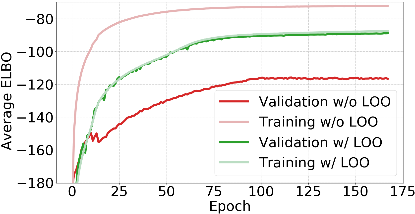
Figure 2: Training and validation ELBO on Dynamic MNIST for Exemplar VAE with and without LOO.

	Exemplar VAE
Dataset	w/ LOO	w/o LOO
MNIST	$-82.35$	$-101.33$
Omniglot	$-105.80$	$-139.12$

Table 1: Log likelihood lower bounds on the test set (nats) for Exemplar VAE with and without leave-one-out (LOO).

Exemplar subsampling. As explained in Sec. 3.2, the Exemplar VAE uses a hyper-parameter $M$ to define the number of exemplars used for estimating the prior. Here, we report the Exemplar VAE’s density estimates as a function of $M$ divided by the number of training data points $N$. We consider $M/N\in\{1.0,0.5,0.2,0.1\}$. All models use LOO, and $M/N=1$ reflects $M=N-1$. Table 2 presents results for MNIST and Omniglot. In all of the following experiments we adopt $M/N=0.5$.

	1	0.5	0.2	0.1
MNIST	$-82.35$	$\mathbf{-82.09}$	$-82.12$	$-82.20$
Omniglot	$-105.80$	$-105.22$	$\mathbf{-104.95}$	$-105.42$

Table 2: Test log likelihood lower bounds (nats) for Exemplar VAE versus fraction of exemplar subsampling.

Method		Dynamic MNIST	Fashion MNIST	Omniglot
VAE w/ Gaussian prior		$-84.45$ $\pm 0.12$	$-228.70$ $\pm 0.15$	$-108.34$ $\pm 0.06$
VAE w/ VampPrior		$-82.43$ $\pm 0.06$	$-227.35$ $\pm 0.05$	$-106.78$ $\pm 0.21$
Exemplar VAE		$-82.09$ $\pm 0.18$	$-226.75$ $\pm 0.07$	$-105.22$ $\pm 0.18$
HVAE w/ Gaussian prior		$-82.39$ $\pm 0.11$	$227.37$ $\pm 0.1$	$-104.92$ $\pm 0.08$
HVAE w/ VampPrior		$-81.56$ $\pm 0.09$	$-226.72$ $\pm 0.08$	$-103.30$ $\pm 0.43$
Exemplar HVAE		$-81.22$ $\pm 0.05$	$-226.53$ $\pm 0.09$	$-102.25$ $\pm 0.43$
ConvHVAE w/ Gaussian prior		$-80.52$ $\pm 0.28$	$-225.38$ $\pm 0.08$	$-98.12$ $\pm 0.17$
ConvHVAE w/ Lars		$-80.30$	$-225.92$	$-97.08$
ConvHVAE w/ SNIS		$-79.91$ $\pm 0.05$	$-225.35$ $\pm 0.07$	N/A
ConvHVAE w/ VampPrior		$-79.67$ $\pm 0.09$	$-224.67$ $\pm 0.03$	$-97.30$ $\pm 0.07$
Exemplar ConvHVAE		$-79.58$ $\pm 0.07$	$-224.63$ $\pm 0.06$	$-96.38$ $\pm 0.24$
PixelSNAIL w/ Gaussian Prior		$-78.20$ $\pm 0.02$	$-223.68$ $\pm 0.03$	$-89.59$ $\pm 0.07$
PixelSNAIL w/ VampPrior		$-77.90$ $\pm 0.02$	$-223.45$ $\pm 0.02$	$-89.50$ $\pm 0.13$
Exemplar PixelSNAIL		$-77.95$ $\pm 0.01$	$-223.26$ $\pm 0.01$	$-89.28$ $\pm 0.12$

Table 3: Density estimation on dynamic MNIST, Fashion MNIST, and Omniglot for different methods and architectures, all with 40-D latent spaces. Log likelihood lower bounds (nats), estimated with IWAE with 5000 samples, are averaged over 5 training runs. For LARS [2] and SNIS [36], the IWAE used 1000 samples; their architectures and training procedures are also somewhat different.

MNIST			Fashion MNIST			Omniglot

CelebA

Figure 3: Given a source exemplar on the top left of each plate, Exemplar VAE samples are generated, showing a significant diversity while preserving properties of the source exemplar.

missing

Figure 4: Interpolation between samples from the CelebA dataset.

5.2 Density Estimation

For each architecture, we compare to a Gaussian prior and a VampPrior, which represent the state-of-the-art among VAEs with a factored variational posterior. For training VAE and HVAE we did not utilize RAT, but for convolutional architectures we used RAT with 10NN search (see Sec. 3.1). Note that the number of nearest neighbors are selected based on computational budget; we believe larger values work better. Table 3 shows that Exemplar VAEs outperform other models in all cases except one. Improvement on Omniglot is greater than on other datasets, which may be due to its significant diversity. One can attempt to increase the number of pseudo-inputs in VampPrior, but this leads to overfitting. As such, we posit that Exemplar VAEs have the potential to more easily scale to large, diverse datasets. Note that training an Exemplar ConHVAE with approximate 10NN search is as efficient as training a ConHVAE with a VampPrior. Also, note that VampPrior [57] showed that a mixture of variational posteriors outperforms a Gaussian mixture prior, and hence we do not directly compare to that baseline.

Fig. 3 shows samples generated from an Exemplar ConvVAE, for which the corresponding exemplars are shown in the top left corner of each plate. These samples highlight the power of Exemplar VAE in maintaining the content of the source exemplar while adding diversity. For MNIST the changes are subtle, but for Fashion MNIST and Omniglot samples show more pronounced variation in style, possibly because those datasets are more diverse.

To assess the scalability of Exemplar VAEs to larger datasets, we train this model on $64\!\times\!64$ CelebA images [40]. Pixel values are modeled using a discretized logistic distribution [34, 53]. Exemplar VAE samples (Figure 3) are high quality with good diversity. Interpolation in the latent space is also effective (Figure 4). More details and quantitative evaluations are provided in the supplementary materials.

5.3 Representation Learning

Exemplar VAE on MNIST	VAE on MNIST

Figure 5: t-SNE visualization of learned latent representations for test points, colored by labels.

Method	MNIST	Fashion MNIST
VAE w/ Gaussian Prior	$2.41$ $\pm 0.27$	$15.90$ $\pm 0.34$
VAE w/ VampPrior	$1.42$ $\pm 0.02$	$12.74$ $\pm 0.18$
Exemplar VAE	$1.13$ $\pm 0.06$	$12.56$ $\pm 0.08$

Table 4: kNN classification error (%) on 40-D unsupervised representations.

We next explore the structure of the latent representation for Exemplar VAE. Fig. 10 shows a t-SNE visualization of the latent representations of MNIST test data for the Exemaplar VAE and for VAE with a Gaussian prior. Test points are colored by their digit label. No labels were used during training. The Exemplar VAE representation appears more meaningful, with tighter clusters than VAE. We also use k-nearest neighbor (kNN) classification performance as a proxy for the representation quality. As is clear from Table 4, Exemplar VAE consistently outperforms other approaches. Results on Omniglot are not reported since the low resolution variant of this dataset does not include class labels. We also counted the number of active dimension in the latent to measure posterior collapse. Section D of supplementary materials shows the superior behavior of Exemplar VAE.

missing

5.4 Generative Data Augmentation

Finally, we ask whether Exemplar VAE is effective in generating augmented data to improve supervised learning. Recent generative models have achieved impressive sample quality and diversity, but limited success in improving discriminative models. Class-conditional models were used to generate training data, but with marginal gains [48]. Techniques for optimizing geometric augmentation policies [11, 39, 25] and adversarial perturbations [20, 43] were more successful for classification.

Here we use the original training data as exemplars, generating extra samples from Exemplar VAE. Class labels of source exemplars are transferred to corresponding generated images, and a combination of real and generated data is used for supervised learning. Each training iteration involves 3 steps:

1. Draw a minibatch ${X}\!=\!\{(\bm{\mathbf{x}}_{i},\ y_{i})\}_{i=1}^{B}$ from training data.

2. For each $\bm{\mathbf{x}}_{i}\in{X}$, draw $\bm{\mathbf{z}}_{i}\sim r_{\phi}(\bm{\mathbf{z}}\mid\bm{\mathbf{x}}_{i})$, and then set $\tilde{\bm{\mathbf{x}}}_{i}=\bm{\mu}_{\phi}(\bm{\mathbf{x}}\mid\bm{\mathbf{z}}_{i})$, which inherits the class label $y_{i}$. This yields a synthetic minibatch $\tilde{X}=\{(\tilde{\bm{\mathbf{x}}}_{i},\ y_{i})\}_{i=1}^{B}$.

3. Optimize the weighted cross entropy: $\mathcal{\ell}=-\sum_{i=1}^{B}\Big{[}\lambda\log p_{\theta}(y_{i}\!\mid\!\bm{\mathbf{x}}_{i})+(1\!-\!\lambda)\log p_{\theta}(y_{i}\!\mid\!\tilde{\bm{\mathbf{x}}}_{i})\Big{]}$

For VAE with Gaussian prior and VampPrior we sampled from variational posterior instead of $r_{\phi}$. We train MLPs with ReLU activations and two hidden layers of 1024 or 8192 units on MNIST and Fashion MNIST. We leverage label smoothing [56] with a parameter of $0.1$. The Exemplar VAEs used for data augmentation have fully connected layers and are not trained with class labels.

Fig.  6 shows Exemplar VAE is more effective than other VAEs for data augmentation. Even small amounts of generative data augmentation improves classifier accuracy. A classifier trained solely on synthetic data achieves better error rates than one trained on the original data. Given $\lambda=0.4$ on MNIST and $\lambda=0.8$ on Fashion MNIST, we train 10 networks on the union of training and validation sets and report average test errors. On permutation invariant MNIST, Exemplar VAE augmentations achieve an average error rate of $0.69\%$. Tables 6 and 6 summarize the results in comparison with previous work. Ladder Networks [54] and Virtual Adversarial Training [43] report error rates of $0.57\%$ and $0.64\%$ on MNIST, using deeper architectures and more complex training procedures.

Method	Hidden layers	Test error
Dropout [55]	$3\!\times\!1024$	$1.25$
Label smoothing [47]	$2\!\times\!1024$	$1.23\scriptsize{\,\pm 0.06}$
Dropconnect [58]	$2\!\times\!800$	$1.20$
VIB [1]	$2\!\times\!1024$	$1.13$
Dropout + MaxNorm [55]	$2\!\times\!8192$	$0.95$
MTC [52]	$2\!\times\!2000$	$0.81$
DBM + DO fine. [55]	$500{\text{-}}500{\text{-}}2K$	$0.79$
Label Smoothing (LS)	$2\!\times\!1024$	$1.23\scriptsize{\,\pm 0.01}$
LS+Exemplar VAE Aug.	$2\!\times\!1024$	$0.77\scriptsize{\,\pm 0.01}$
Label Smoothing	$2\!\times\!8196$	$1.17\scriptsize{\,\pm 0.01}$
LS+Exemplar VAE Aug.	$2\!\times\!8192$	$\mathbf{0.69}\scriptsize{\,\pm 0.01}$

Table 5: Test error (%) on permutation invariant MNIST from [55, 47, 58, 1, 52], and our results with and without generative data augmentation.

Method	Hidden layers	Test error
Label Smoothing	$2\!\times\!1024$	$8.96\scriptsize{\,\pm 0.04}$
LS+Exemplar VAE Aug.	$2\!\times\!1024$	$8.46\scriptsize{\,\pm 0.04}$
Label Smoothing	$2\!\times\!8196$	$8.56\scriptsize{\,\pm 0.03}$
LS+Exemplar VAE Aug.	$2\!\times\!8192$	$\mathbf{8.16}\scriptsize{\,\pm 0.03}$

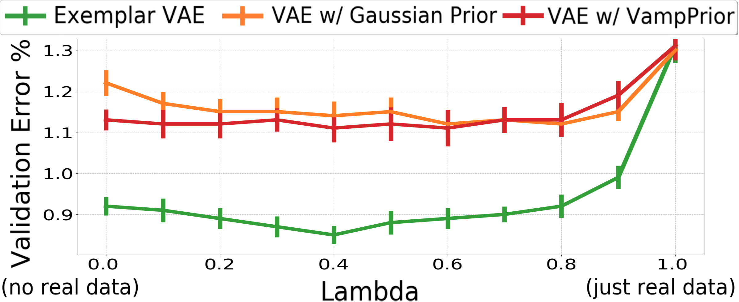
Table 6: Test error (%) on permutaion invariant Fashion MNIST.

Figure 6: MNIST validation error versus $\lambda$, which controls the relative balance of real and augmented data, for different generative models.

6 Conclusion

We develop a framework for exemplar based generative modeling called the Exemplar VAE. We present two effective regularization techniques for Exemplar VAEs, and an efficient learning algorithm based on approximate nearest neighbor search. The effectiveness of the Exemplar VAE on density estimation, representation learning, and data augmentation for supervised learning is demonstrated. The development of Exemplar VAEs opens up interesting future research directions such as application to NLP (cf. [24]) and other discrete data, further exploration of unsupervised data augmentation, and extentions to other generative models such as Normalizing Flows and GANs.

Broader Impact Statement

The ideas described in our paper concern the development of a new fundamental class of unsupervised learning algorithm, rather than an application per se. One important property of the method stems from it’s non-parametric form, i.e., as an exemplar-based model. As such, rather than having the "model" represented solely in the weights of an amorphous non-linear neural network, in our case much of the model is expressed directly in terms of the dataset of exemplars. As such, the model is somewhat more interpretable and may facilitate the examination or discovery of bias, which has natural social and ethical implications. Beyond that, the primary social and ethical implications will derive from the way in which the algorithm is applied in different domains.

Funding Disclosure

This research was supported in part by an NSERC Discovery Grant to DJF, and by Province of Ontario, the Government of Canada, through NSERC and CIFAR, and companies sponsoring the Vector Institute.

Appendix A Exemplar VAE samples

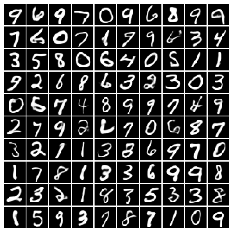
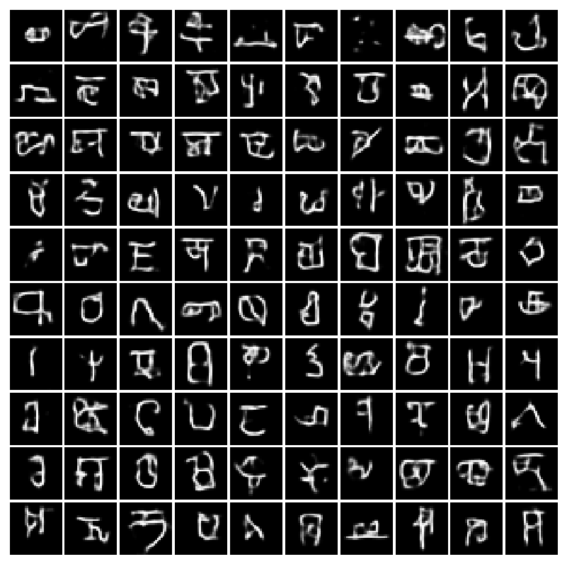
MNIST	Fashion MNIST	Omniglot
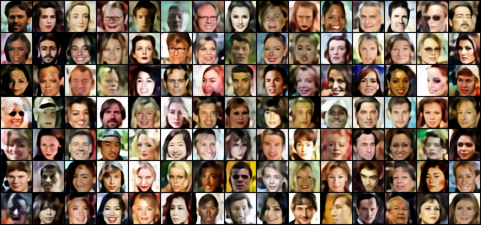
CelebA

Figure 7: Random samples drawn from Exemplar VAEs trained on different datasets.

Appendix B Exemplar conditioned samples

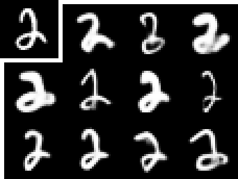
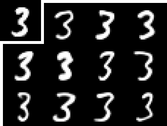
Figure 8: Given the input exemplar on the top left of each plate, $11$ exemplar conditioned samples using Exemplar VAE are generated and shown.

missing

Appendix C Retrieval Augmented Training

Algorithm 1

  Input: Training dataset $\mathcal{X}=\{\bm{\mathbf{x}}_{n}\}_{n=1}^{N}$

  Define Cache:

    initialize cache = []

    $\mathrm{insert}(i,\bm{c})$: insert value $\bm{c}$ with index $i$ into cache

    $\mathrm{update}(i,\bm{c})$: update the value of index $i$ to $\bm{c}$

    $\mathrm{kNN}(\bm{c})$: return indices of kNNs of $\bm{c}$ in cache

  for $n$  in  $\{1,\ldots,N\}$ do $\mathrm{Cache.insert}(n,\bm{\mu}_{\phi}(\bm{\mathbf{x}}_{n}))$

  for epoch  in  $\{1,\ldots,L\}$ do

   for $i$  in  $\{1,\ldots,N\}$ do

    $\pi\sim\Pi^{N,i}_{M}$ to obtain a set of $M$ exemplar indices

    $\bm{\mu}_{i},\Lambda_{i}=\bm{\mu}_{\phi}(\bm{\mathbf{x}}_{i}),\Lambda_{\phi}(\bm{\mathbf{x}}_{i})$

    $\bm{\epsilon}\sim\mathcal{N}(0,I_{d_{z}\times d_{z}})$

    $\bm{\mathbf{z}}=\bm{\mu}_{i}+\Lambda_{i}^{1/2}\bm{\epsilon}$

    $\mathrm{kNN}=\mathrm{Cache.kNN}(\bm{\mu}_{i})\cap\ \pi$

    for $j$  in  $\mathrm{kNN}$ do $\bm{\mu}_{j}=\bm{\mu}_{\phi}(\bm{\mathbf{x}}_{j})$

    $m(\bm{\mathbf{z}})=\frac{1}{M}\sum_{j\in\mathrm{kNN}}\mathcal{N}(\bm{\mathbf{z}}\!\mid\!\bm{\mu}_{j},\sigma^{2})$

    $\mathrm{ELBO}\!=\!\log p_{\theta}(\bm{\mathbf{x}}\!\mid\!\bm{\mathbf{z}})\!-\!\log\mathcal{N}(\bm{\mathbf{z}}\!\mid\!\bm{\mu}_{i},\Lambda_{i})\!+\!\log r(\bm{\mathbf{z}})$

    Gradient ascend on $\mathrm{ELBO}$ to update $\phi$, $\theta$, and $\sigma^{2}$

    $\mathrm{Cache.update}(i,\bm{\mu}_{i})$

    for $j$  in  $\mathrm{kNN}$ do $\mathrm{Cache.update}(j$, $\bm{\mu}_{j})$

Appendix D Number of Active Dimensions in the Latent Space

The problem of posterior collapse [5, 41], resulting in a number of inactive dimensions in the latent space of a VAE. We investigate this phenomena by counting the number of active dimensions based on a metric proposed by Burda et. al [6]. This metric computes the variance of the mean of the latent encoding of the data points in each dimension of the latent space, $\mathrm{Var}(\mu_{\phi}(\bm{\mathbf{x}})_{i})$, where $\bm{\mathbf{x}}$ is sampled from the dataset. If the computed variance is above a certain threshold, then that dimension is considered active. The proposed threshold by [2] is $0.01$ and we use the same value. We observe that the Exemplar VAE has the largest number of active dimensions in all cases except one. In the case of ConvHVAE and PixelSNAIL, the gap between Exemplar VAE and other methods is more considerable.

	Number of active dimensions out of $40$
Model	Dynamic MNIST	Fashion MNIST	Omniglot
VAE w/ Gaussian prior	$24.0$$\pm 0.63$	$26.0$$\pm 1.1$	$35.2$$\pm 0.4$
VAE w/ Vampprior	$27.6$$\pm 1.36$	$35.25$$\pm 1.3$	$40.0$$\pm 0.0$
Exemplar VAE	$29.4$$\pm 0.49$	$36.0$$\pm 1.41$	$40.0$$\pm 0.0$
HVAE w/ Gaussian prior	$15.0$$\pm 0.63$	$12.4$$\pm 0.8$	$24.8$$\pm 1.83$
HVAE w/ VampPrior	$20.4$$\pm 0.49$	$23.2$$\pm 1.47$	$39.0$$\pm 0.89$
Exemplar HVAE	$21.6$$\pm 0.49$	$28.6$$\pm 0.8$	$38.6$$\pm 1.5$
ConvHVAE w/ Gaussian prior	$19.8$$\pm 2.93$	$15.4$$\pm 2.65$	$39.2$$\pm 1.6$
ConvHVAE w/ VampPrior	$19.0$$\pm 1.55$	$19.25$$\pm 0.83$	$39.8$$\pm 0.4$
Exemplar ConvHVAE	$25.8$$\pm 3.66$	$33.6$$\pm 7.86$	$40.0$$\pm 0.0$
PixelSNAIL w/ Gaussian prior	$4.6$$\pm 0.36$	$2.4$$\pm 0.22$	$0.0$$\pm 0.0$
PixelSNAIL w/ VampPrior	$17.2$$\pm 1.39$	$30.6$$\pm 0.73$	$9.50$$\pm 4.48$
Exemplar PixelSNAIL	$25.8$$\pm 0.66$	$37.2$$\pm 0.87$	$25.5$$\pm 1.82$

Table 7: The number of active dimensions computed based on a metric proposed by Burda et. al [6]. This metric considers a latent dimension active if the variance of its mean over the dataset is higher than $0.01$. For hierarchical architectures the reported number is for the $\bm{\mathbf{z}}_{2}$ which is the highest stochastic layer.

Appendix E CelebA Quantitative Results

Model	bits per dim
VAE w/ Gaussian Prior	$5.825$
Exemplar VAE	$5.780$

Table 8: Numerical Evaluations for CelebA

Appendix F Derivation of Eqn. (5)

$$\log p(\bm{\mathbf{x}};X,\theta,\phi) ~{}=~{}\log\sum_{n=1}^{N}\frac{1}{N}\int_{z}{r_{\phi}(\bm{\mathbf{z}}\mid\bm{\mathbf{x}}_{n})\,p_{\theta}(\bm{\mathbf{x}}\mid\bm{\mathbf{z}})}\,d\bm{\mathbf{z}}$$ (13)

$$~{}=~{}\log\int_{z}p_{\theta}(\bm{\mathbf{x}}\mid\bm{\mathbf{z}})\sum\nolimits_{n=1}^{N}\frac{1}{N}{r_{\phi}(\bm{\mathbf{z}}\mid\bm{\mathbf{x}}_{n})\,}\,d\bm{\mathbf{z}}$$ (14)

$$~{}=~{}\log\int_{z}\frac{q_{\phi}(\bm{\mathbf{z}}\mid\bm{\mathbf{x}})p_{\theta}(\bm{\mathbf{x}}\mid\bm{\mathbf{z}})\sum\nolimits_{n=1}^{N}\frac{1}{N}{r_{\phi}(\bm{\mathbf{z}}\mid\bm{\mathbf{x}}_{n})\,}}{q_{\phi}(\bm{\mathbf{z}}|\bm{\mathbf{x}})}\,d\bm{\mathbf{z}}$$ (15)

$$~{}\geq~{}\underbrace{\mathop{\mathbb{E}}_{q_{\phi}(\bm{\mathbf{z}}\mid\bm{\mathbf{x}})}\!\!\!\log p_{\theta}(\bm{\mathbf{x}}\!\mid\!\bm{\mathbf{z}})}_{\mathrm{reconstruction}}-\!\!\underbrace{\mathop{\mathbb{E}}_{q_{\phi}(\bm{\mathbf{z}}\mid\bm{\mathbf{x}})}\log\frac{q_{\phi}(\bm{\mathbf{z}}\mid\bm{\mathbf{x}})}{\sum\nolimits_{n=1}^{N}r_{\phi}(\bm{\mathbf{z}}\mid\bm{\mathbf{x}}_{n})/N}}_{\mathrm{KL~{}term}}$$ (16)

$$~{}=~{}O(\theta,\phi;\bm{\mathbf{x}},X).$$ (17)

Appendix G Iterative generation

The exemplar VAE generates a new sample by stochastically transforming an exemplar. The newly generated data point can also be used as an exemplar, and we can repeat this procedure again and again. This kind of generation bears some similarity to MCMC for sampling from energy-based models. Figure 9 shows how samples evolve and consistently stay near the manifold of MNIST digits. We can apply the same procedure starting from a noisy input image as an exemplar. Figure 10 shows that the model is able to quickly transform the noisy images into samples that resemble real MNIST images.

Figure 9: Iterative generation starting from a training data point. Samples generated from an Exemplar VAE starting from a training data point, and then reusing the generated data as exemplars for the next round of generation (left to right).

Figure 10: Iterative generation starting from a noise input (left to right).

Appendix H Computation and Memory Complexity

The cost of training Exemplar VAE is similar to that of VampPrior, which uses mixture of variational posteriors. When the number of exemplars per minibatch is equal to the number of pseudo-inputs in VampPrior the computational complexity is very similar. For example, for ConvHVAE on Omniglot, VampPrior with 1000 pseudo-inputs takes 58s/epoch and Exemplar VAE with a minibatch of 100 and 10 NNs takes 51s/epoch on a single Nvidia T4 GPU (it runs faster because we use an isotropic gaussians in our prior). In case of ConvHVAE on MNIST and FashionMNIST VampPrior with 500 pseudo inputs takes 82s/epoch vs 107s/epoch for Exemplar VAE with batch size of 100 and 10 NNs per data point. Regarding memory complexity, Exemplar VAE stores low-dimensional latent embeddings. By comparison, VampPrior stores pseudo inputs with the same dimentionality as the input data, which can be problematic in case of high dimensional data.

Appendix I Reconstruction vs. KL

Table 9 shows the value of KL and the reconstruction terms of ELBO, computed based on a single sample from the variational posterior, averaged across test set. On non-autoregressive architectures, these numbers show that not only the exemplar VAE improves the KL term, but also the reconstruction terms are comparable with the VampPrior. On PixelSNAIL, these numbers confirm that Exemplar PixelSNAIL utilize the latent space better.

	Dynamic MNIST		Fashion MNIST		Omniglot
Model	KL	Neg.Reconst.	KL	Neg. Reconst.	KL	Neg. Reconst.
VAE w/ Gaussian prior	$25.54$$\pm 0.12$	$63.06$$\pm 0.11$	$18.38$$\pm 0.11$	$213.21$$\pm 0.18$	$32.97$$\pm 0.2$	$82.3$$\pm 0.21$
VAE w/ VampPrior	$25.14$$\pm 0.16$	$60.79$$\pm 0.13$	$18.44$$\pm 0.06$	$211.37$$\pm 0.04$	$34.17$$\pm 0.22$	$79.49$$\pm 0.18$
Exemplar VAE	$24.82$$\pm 0.22$	$61.00$$\pm 0.13$	$18.32$$\pm 0.08$	$211.10$$\pm 0.1$	$32.66$$\pm 0.27$	$80.25$$\pm 0.62$
HVAE w/ Gaussian prior	$26.80$$\pm 0.13$	$59.80$$\pm 0.11$	$19.08$$\pm 0.05$	$211.18$$\pm 0.14$	$36.07$$\pm 0.12$	$75.96$$\pm 0.12$
HVAE w/ VampPrior	$26.69$$\pm 0.1$	$58.46$$\pm 0.06$	$19.27$$\pm 0.15$	$210.04$$\pm 0.2$	$38.39$$\pm 0.16$	$72.42$$\pm 0.34$
Exemplar HVAE	$26.41$$\pm 0.17$	$58.48$$\pm 0.16$	$18.96$$\pm 0.15$	$210.40$$\pm 0.16$	$36.76$$\pm 0.25$	$73.35$$\pm 0.63$
ConvHVAE w/ Gaussian prior	$26.58$$\pm 0.27$	$57.64$$\pm 0.57$	$20.34$$\pm 0.04$	$208.11$$\pm 0.06$	$38.90$$\pm 0.22$	$67.22$$\pm 0.1$
ConvHVAE w/ VampPrior	$26.57$$\pm 0.17$	$56.18$$\pm 0.03$	$20.65$$\pm 0.19$	$206.64$$\pm 0.15$	$38.95$$\pm 0.17$	$66.38$$\pm 0.3$
Exemplar ConvHVAE	$26.41$$\pm 0.25$	$56.14$$\pm 0.27$	$20.46$$\pm 0.23$	$207.18$$\pm 0.38$	$37.48$$\pm 0.37$	$66.62$$\pm 0.32$
PixelSNAIL w/ Gaussian prior	$5.73$$\pm 0.09$	$72.92$$\pm 0.08$	$4.68$$\pm 0.16$	$219.51$$\pm 0.16$	$0.01$$\pm 0.0$	$89.57$$\pm 0.07$
PixelSNAIL w/ VampPrior	$7.17$$\pm 0.18$	$71.23$$\pm 0.19$	$6.07$$\pm 0.07$	$218.00$$\pm 0.08$	$1.07$$\pm 0.42$	$88.54$$\pm 0.47$
Exemplar PixelSNAIL	$10.94$$\pm 0.03$	$67.89$$\pm 0.02$	$10.35$$\pm 0.07$	$213.95$$\pm 0.08$	$10.03$$\pm 0.14$	$80.19$$\pm 0.06$

Table 9: KL and reconstruction part of ELBO averaged over test set by a single sample from posterior.

Appendix J t-SNE visualization of Fashion MNIST latent space

We showed t-SNE visualization of MNIST latent space in the figure 5. Here we show the same plot for fashion-mnist. Interestingly, some classes are very close to each other (Pullover-shirt-dress) and transition between them happens very smoothly while some other classes are more separated.

Exemplar VAE on Fashion MNIST	VAE on Fashion MNIST

Table 10: t-SNE visualization of learned latent representations for Fashion-MNIST test points, colored by labels.

Appendix K Experimental Details

K.1 Architectures

All of the neural network architectures are based on the VampPrior of Tomczak & Welling [57] except PixelSNAIL. We leave tuning the architecture of Exemplar VAEs to future work. To describe the network architectures, we follow the notation of LARS [2]. Neural network layers used are either convolutional (denoted CNN) or fully-connected (denoted MLP), and the number of units are written inside a bracket separated by a dash (e.g., MLP[300-784] means a fully-connected layer with 300 input units and 784 output units). We use curly bracket to show concatenation. $d_{z}$ refers to the dimensionality of the latent space.

a) VAE:

$$q_{\phi}(\bm{\mathbf{z}}\mid\bm{\mathbf{x}}) = \mathcal{N}(\bm{\mathbf{z}};~{}\mu_{\bm{\mathbf{z}}}(\bm{\mathbf{x}}),\Lambda_{\bm{\mathbf{z}}}(\bm{\mathbf{x}}))$$

$$p_{\phi}(\bm{\mathbf{x}}\mid\bm{\mathbf{z}}) = \textrm{Bernoulli}(x,\mu_{\bm{\mathbf{x}}}(\bm{\mathbf{z}}))$$

$$\textrm{Encoder}_{\bm{\mathbf{z}}}(\bm{\mathbf{x}}) = \textrm{MLP}~{}[784-300-300]$$

$$\log\Lambda_{\bm{\mathbf{z}}}^{2}(\bm{\mathbf{x}}) = \textrm{MLP}[\textrm{Encoder}_{\bm{\mathbf{z}}}(x)-d_{\bm{\mathbf{z}}}]$$

$$\mu_{\bm{\mathbf{z}}}(\bm{\mathbf{x}}) = \textrm{MLP}[\textrm{Encoder}_{\bm{\mathbf{z}}}(x)-d_{\bm{\mathbf{z}}}]$$

$$\mu_{\bm{\mathbf{x}}}(\bm{\mathbf{z}}) = \textrm{MLP}[d_{\bm{\mathbf{z}}}-300-300-784]$$

b) HVAE:

$$q_{\phi}(\bm{\mathbf{z}}_{2}\mid\bm{\mathbf{x}}) = \mathcal{N}(\bm{\mathbf{z}}_{2};~{}\mu_{\bm{\mathbf{z}}_{2}}(\bm{\mathbf{x}}),\Lambda_{\bm{\mathbf{z}}_{2}}(\bm{\mathbf{x}}))$$

$$q_{\phi}(\bm{\mathbf{z}}_{1}\mid\bm{\mathbf{x}},~{}\bm{\mathbf{z}}_{2}) = \mathcal{N}(\bm{\mathbf{z}}_{1};~{}\mu_{\bm{\mathbf{z}}_{1}}(\bm{\mathbf{x}},~{}\bm{\mathbf{z}}_{2}),\Lambda_{\bm{\mathbf{z}}_{1}}(\bm{\mathbf{x}},~{}\bm{\mathbf{z}}_{2}))$$

$$p_{\phi}(\bm{\mathbf{z}}_{1}\mid\bm{\mathbf{z}}_{2}) = \mathcal{N}(\bm{\mathbf{z}}_{1};~{}\hat{\mu}_{\bm{\mathbf{z}}_{1}}(\bm{\mathbf{z}}_{2}),\hat{\Lambda}_{\bm{\mathbf{z}}_{1}}(\bm{\mathbf{z}}_{2}))$$

$$p_{\phi}(\bm{\mathbf{x}}\mid\bm{\mathbf{z}}_{1},~{}\bm{\mathbf{z}}_{2}) = \textrm{Bernoulli}(\bm{\mathbf{x}},\mu_{\bm{\mathbf{x}}}(\bm{\mathbf{z}}_{1},~{}\bm{\mathbf{z}}_{2}))$$

$$\textrm{Encoder}_{\bm{\mathbf{z}}_{2}}(\bm{\mathbf{x}}) = \textrm{MLP}[784-300-300]$$

$$\log\Lambda_{\bm{\mathbf{z}}_{2}}^{2}(\bm{\mathbf{x}}) = \textrm{MLP}[\textrm{Encoder}_{\bm{\mathbf{z}}_{2}}(\bm{\mathbf{x}})-d_{\bm{\mathbf{z}}_{2}}]$$

$$\mu_{\bm{\mathbf{z}}_{2}}(\bm{\mathbf{x}}) = \textrm{MLP}[\textrm{Encoder}_{\bm{\mathbf{z}}_{2}}(\bm{\mathbf{x}})-d_{\bm{\mathbf{z}}_{2}}]$$

$$\textrm{Encoder}_{\bm{\mathbf{z}}_{1}}(\bm{\mathbf{x}},\bm{\mathbf{z}}_{2}) = \textrm{MLP}[\{\textrm{MLP}[d_{\bm{\mathbf{z}}_{2}}-300],\textrm{MLP}[784-300]\}-300]$$

$$\log\Lambda_{\bm{\mathbf{z}}_{1}}^{2}(\bm{\mathbf{x}},\bm{\mathbf{z}}_{2}) = \textrm{MLP}[\textrm{Encoder}_{\bm{\mathbf{z}}_{1}}(\bm{\mathbf{x}},\bm{\mathbf{z}}_{2})-d_{\bm{\mathbf{z}}_{1}}]$$

$$\mu_{\bm{\mathbf{z}}_{1}}(\bm{\mathbf{x}},\bm{\mathbf{z}}_{2}) = \textrm{MLP}[\textrm{Encoder}_{\bm{\mathbf{z}}_{1}}(\bm{\mathbf{x}},\bm{\mathbf{z}}_{2})-d_{\bm{\mathbf{z}}_{1}}]$$

$$\textrm{Decoder}_{\bm{\mathbf{z}}_{1}}(\bm{\mathbf{z}}_{2}) = \textrm{MLP}[d_{\bm{\mathbf{z}}_{2}}-300-300]$$

$$\log\hat{\Lambda}_{\bm{\mathbf{z}}_{1}}^{2}(\bm{\mathbf{z}}_{2}) = \textrm{MLP}[\textrm{Decoder}_{\bm{\mathbf{z}}_{1}}(\bm{\mathbf{z}}_{2})-d_{\bm{\mathbf{z}}_{1}}]$$

$$\hat{\mu}_{\bm{\mathbf{z}}_{1}}(\bm{\mathbf{z}}_{2}) = \textrm{MLP}[\textrm{Decoder}_{\bm{\mathbf{z}}_{1}}(\bm{\mathbf{z}}_{2})-d_{\bm{\mathbf{z}}_{1}}]$$

$$\mu_{\bm{\mathbf{x}}}(\bm{\mathbf{z}}_{1},\bm{\mathbf{z}}_{2}) = MLP[\{\textrm{MLP}[d_{\bm{\mathbf{z}}_{1}}-300],\textrm{MLP}[d_{\bm{\mathbf{z}}_{2}}-300]\}-300-784]$$

c) ConvHVAE: The generative and variational posterior distributions are identical to HVAE.

$$\textrm{Encoder}_{\bm{\mathbf{z}}_{2}}(\bm{\mathbf{x}}) = \textrm{CNN}[28\times 28\times 1-32\times 32\times 32-12\times 12\times 32-12\times 12\times 64-7\times 7\times 64$$

$$-7\times 7\times 6]$$

$$\log\Lambda_{\bm{\mathbf{z}}_{2}}^{2}(\bm{\mathbf{x}}) = \textrm{MLP}[\textrm{Encoder}_{\bm{\mathbf{z}}_{2}}(\bm{\mathbf{x}})-d_{\bm{\mathbf{z}}_{2}}]$$

$$\mu_{\bm{\mathbf{z}}_{2}}(\bm{\mathbf{x}}) = \textrm{MLP}[\textrm{Encoder}_{\bm{\mathbf{z}}_{2}}(\bm{\mathbf{x}})-d_{\bm{\mathbf{z}}_{2}}]$$

$$\textrm{ConvEncoder}_{\bm{\mathbf{z}}_{1}}(\bm{\mathbf{x}}) = \textrm{CNN}[28\times 28\times 1-32\times 32\times 32-12\times 12\times 32-12\times 12\times 64-7\times 7\times 64-7\times 7\times 6]$$

$$\textrm{Encoder}_{\bm{\mathbf{z}}_{1}}(\bm{\mathbf{x}},\bm{\mathbf{z}}_{2}) = \textrm{MLP}[\{\textrm{MLP}[d_{\bm{\mathbf{z}}_{2}}$$

$$-7\times 7\times 6],\textrm{ConvEncoder}_{\bm{\mathbf{z}}_{1}}(\bm{\mathbf{x}})\}-300]$$

$$\log\Lambda_{\bm{\mathbf{z}}_{1}}^{2}(\bm{\mathbf{x}},\bm{\mathbf{z}}_{2}) = \textrm{MLP}[\textrm{Encoder}_{\bm{\mathbf{z}}_{1}}(\bm{\mathbf{x}},\bm{\mathbf{z}}_{2})-d_{\bm{\mathbf{z}}_{1}}]$$

$$\mu_{\bm{\mathbf{z}}_{1}}(\bm{\mathbf{x}},\bm{\mathbf{z}}_{2}) = \textrm{MLP}[\textrm{Encoder}_{\bm{\mathbf{z}}_{1}}(\bm{\mathbf{x}},\bm{\mathbf{z}}_{2})-d_{\bm{\mathbf{z}}_{1}}]$$

$$\textrm{Decoder}_{\bm{\mathbf{z}}_{1}}(\bm{\mathbf{z}}_{2}) = \textrm{MLP}[d_{\bm{\mathbf{z}}_{2}}-300-300]$$

$$\log\hat{\Lambda}_{\bm{\mathbf{z}}_{1}}^{2}(\bm{\mathbf{z}}_{2}) = \textrm{MLP}[\textrm{Decoder}_{\bm{\mathbf{z}}_{1}}(\bm{\mathbf{z}}_{2})-d_{\bm{\mathbf{z}}_{1}}]$$

$$\hat{\mu}_{\bm{\mathbf{z}}_{1}}(\bm{\mathbf{z}}_{2}) = \textrm{MLP}[\textrm{Decoder}_{\bm{\mathbf{z}}_{1}}(\bm{\mathbf{z}}_{2})-d_{\bm{\mathbf{z}}_{1}}]$$

$$\textrm{MLPDecoder}_{\bm{\mathbf{x}}}(\bm{\mathbf{z}}_{1},\bm{\mathbf{z}}_{2}) = \textrm{MLP}[\{\textrm{MLP}[d_{\bm{\mathbf{z}}_{1}}-300],\textrm{MLP}[d_{\bm{\mathbf{z}}_{2}}-300]\}-784]$$

$$\textrm{ConvDecoder}_{\bm{\mathbf{x}}} = \textrm{CNN}[28\times 28\times 64-28\times 28\times 64-28\times 28\times 64-28\times 28\times 64-28\times 28\times 1]$$

$$\mu_{\bm{\mathbf{x}}}(\bm{\mathbf{z}}_{1},\bm{\mathbf{z}}_{2}) = [\textrm{MLPDecoder}_{\bm{\mathbf{x}}}(\bm{\mathbf{z}}_{1},\bm{\mathbf{z}}_{2})-\textrm{ConvDecoder}_{\bm{\mathbf{x}}}]$$

d) PixelSNAIL HVAE: The generative and variational posterior distributions are identical to HVAE.

$$\textrm{Encoder}_{\bm{\mathbf{z}}_{2}}(\bm{\mathbf{x}}) = \textrm{CNN}[28\times 28\times 1-32\times 32\times 32-12\times 12\times 32-12\times 12\times 64$$

$$-7\times 7\times 64-7\times 7\times 6]$$

$$\log\Lambda_{\bm{\mathbf{z}}_{2}}^{2}(\bm{\mathbf{x}}) = \textrm{MLP}[\textrm{Encoder}_{\bm{\mathbf{z}}_{2}}(\bm{\mathbf{x}})-d_{\bm{\mathbf{z}}_{2}}]$$

$$\mu_{\bm{\mathbf{z}}_{2}}(\bm{\mathbf{x}}) = \textrm{MLP}[\textrm{Encoder}_{\bm{\mathbf{z}}_{2}}(\bm{\mathbf{x}})-d_{\bm{\mathbf{z}}_{2}}]$$

$$\textrm{ConvEncoder}_{\bm{\mathbf{z}}_{1}}(\bm{\mathbf{x}}) = \textrm{CNN}[28\times 28\times 1-32\times 32\times 32-12\times 12\times 32-12\times 12\times 64$$

$$-7\times 7\times 64-7\times 7\times 6]$$

$$\textrm{Encoder}_{\bm{\mathbf{z}}_{1}}(\bm{\mathbf{x}},\bm{\mathbf{z}}_{2}) = \textrm{MLP}[\{\textrm{MLP}[d_{\bm{\mathbf{z}}_{2}}-7\times 7\times 6],\textrm{ConvEncoder}_{\bm{\mathbf{z}}_{1}}(\bm{\mathbf{x}})\}-300]$$

$$\log\Lambda_{\bm{\mathbf{z}}_{1}}^{2}(\bm{\mathbf{x}},\bm{\mathbf{z}}_{2}) = \textrm{MLP}[\textrm{Encoder}_{\bm{\mathbf{z}}_{1}}(\bm{\mathbf{x}},\bm{\mathbf{z}}_{2})-d_{\bm{\mathbf{z}}_{1}}]$$

$$\mu_{\bm{\mathbf{z}}_{1}}(\bm{\mathbf{x}},\bm{\mathbf{z}}_{2}) = \textrm{MLP}[\textrm{Encoder}_{\bm{\mathbf{z}}_{1}}(\bm{\mathbf{x}},\bm{\mathbf{z}}_{2})-d_{\bm{\mathbf{z}}_{1}}]$$

$$\textrm{Decoder}_{\bm{\mathbf{z}}_{1}}(\bm{\mathbf{z}}_{2}) = \textrm{MLP}[d_{\bm{\mathbf{z}}_{2}}-300-300]$$

$$\log\hat{\Lambda}_{\bm{\mathbf{z}}_{1}}^{2}(\bm{\mathbf{z}}_{2}) = \textrm{MLP}[\textrm{Decoder}_{\bm{\mathbf{z}}_{1}}(\bm{\mathbf{z}}_{2})-d_{\bm{\mathbf{z}}_{1}}]$$

$$\hat{\mu}_{\bm{\mathbf{z}}_{1}}(\bm{\mathbf{z}}_{2}) = \textrm{MLP}[\textrm{Decoder}_{\bm{\mathbf{z}}_{1}}(\bm{\mathbf{z}}_{2})-d_{\bm{\mathbf{z}}_{1}}]$$

$$\textrm{MLPDecoder}_{\bm{\mathbf{x}}}(\bm{\mathbf{z}}_{1},\bm{\mathbf{z}}_{2},\bm{\mathbf{x}}) = \{\textrm{MLP}[d_{\bm{\mathbf{z}}_{1}}-784],\textrm{MLP}[d_{\bm{\mathbf{z}}_{2}}-784],\bm{\mathbf{x}}\}$$

$$\textrm{AutoRegressiveDecoder}_{\bm{\mathbf{x}}} = [\textrm{ResNet-MaskedCNN}[28\times 28\times 64]\times 4$$

$$-\textrm{Self-Attention}-\textrm{MaskedCNN}[28\times 28\times 1]]$$

$$\mu_{\bm{\mathbf{x}}}(\bm{\mathbf{z}}_{1},\bm{\mathbf{z}}_{2}) = [\textrm{MLPDecoder}_{\bm{\mathbf{x}}}(\bm{\mathbf{z}}_{1},\bm{\mathbf{z}}_{2},\bm{\mathbf{x}})-\textrm{AutoRegressiveDecoder}_{\bm{\mathbf{x}}}]$$

e) CelebA Architecture:

$$q_{\phi}(\bm{\mathbf{z}}\mid\bm{\mathbf{x}}) = \mathcal{N}(\bm{\mathbf{z}};~{}\mu_{\bm{\mathbf{z}}}(\bm{\mathbf{x}}),\Lambda_{\bm{\mathbf{z}}}(\bm{\mathbf{x}}))$$

$$p_{\phi}(\bm{\mathbf{x}}\mid\bm{\mathbf{z}}) = \textrm{Discretized\_Logistic}(x,\mu_{\bm{\mathbf{x}}}(\bm{\mathbf{z}}),\sigma^{2})$$

$$\textrm{Encoder}_{\bm{\mathbf{z}}}(\bm{\mathbf{x}}) = \textrm{CNN}~{}[64\times 64\times 3-32\times 32\times 64-16\times 16\times 128-8\times 8\times 256-4\times 4\times 512]$$

$$\log\Lambda_{\bm{\mathbf{z}}}^{2}(\bm{\mathbf{x}}) = \textrm{MLP}[\textrm{Encoder}_{\bm{\mathbf{z}}}(x)-d_{\bm{\mathbf{z}}}]$$

$$\mu_{\bm{\mathbf{z}}}(\bm{\mathbf{x}}) = \textrm{MLP}[\textrm{Encoder}_{\bm{\mathbf{z}}}(x)-d_{\bm{\mathbf{z}}}]$$

$$\mu_{\bm{\mathbf{x}}}(\bm{\mathbf{z}}) = \textrm{CNN}[8\times 8\times 512-16\times 16\times 256-32\times 32\times 128-64\times 64\times 64-64\times 64\times 3]$$

As the activation function, the gating mechanism of [13] is used throughout. So for each layer we have two parallel branches where the sigmoid of one branch is multiplied by the output of the other branch. In ConvHVAE the kernel size of the first layer of $\textrm{Encoder}_{\bm{\mathbf{z}}_{2}}(x)$ is 7 and the third layer used kernel size of 5. The last layer of $\textrm{ConvDecoder}_{\bm{\mathbf{x}}}$ used kernel size of 1 and all the other layers used $3\times 3$ kernels. For CelebA we used kernel size of 5 for each layer and combination of batch norm and ELU activation after each convolution layer.

K.2 Hyper-parameters

We use Graident Normalized Adam [61] with Learning rate of $5e-4$ and minibatch size of $100$ for all of the datasets. For gray-scale datasets We dynamically binarize each training data, but we do not binarize the exemplars that serve as the prior. We utilize early stopping for training VAEs, where we stopped the training if for $50$ consecutive epochs the validation ELBO does not improve. We use 40 dimensional latent spaces for gray-scale datasets while using 128 dimensional latent for CelebA. To limit the computation costs of convolutional architectures, we considered kNN based on euclidean distance in the latent space, where $k$ set to $10$ for gray-scale datasets and $5$ for CelebA. The number of exemplars set to the half of the training data except in the ablation study section.

Appendix L Misclassified MNIST Digits

A classifier trained using exemplar augmentation reached average error of $0.69\%$. Here we show the test examples misclassified.

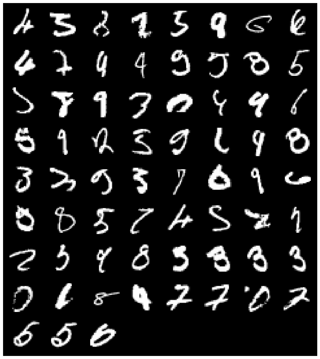
Figure 11: Misclassified images from MNIST test set for a two layer MLP trained with Exemplar VAE augmentation.

missing

References

- [1] Alexander A Alemi, Ian Fischer, Joshua V Dillon, and Kevin Murphy. Deep variational information bottleneck. arXiv:1612.00410, 2016.
- [2] Matthias Bauer and Andriy Mnih. Resampled priors for variational autoencoders. arXiv:1810.11428, 2018.
- [3] David M Blei, Alp Kucukelbir, and Jon D McAuliffe. Variational inference: A review for statisticians. Journal of the American Statistical Association, 2017.
- [4] Jörg Bornschein, Andriy Mnih, Daniel Zoran, and Danilo Jimenez Rezende. Variational memory addressing in generative models. NeurIPS, 2017.
- [5] Samuel R Bowman, Luke Vilnis, Oriol Vinyals, Andrew M Dai, Rafal Jozefowicz, and Samy Bengio. Generating sentences from a continuous space. arXiv:1511.06349, 2015.
- [6] Yuri Burda, Roger Grosse, and Ruslan Salakhutdinov. Importance weighted autoencoders. arXiv:1509.00519, 2015.
- [7] Ricky T. Q. Chen, Xuechen Li, Roger Grosse, and David Duvenaud. Isolating sources of disentanglement in variational autoencoders. Advances in Neural Information Processing Systems, 2018.
- [8] Xi Chen, Diederik P Kingma, Tim Salimans, Yan Duan, Prafulla Dhariwal, John Schulman, Ilya Sutskever, and Pieter Abbeel. Variational lossy autoencoder. arXiv:1611.02731, 2016.
- [9] Xi Chen, Nikhil Mishra, Mostafa Rohaninejad, and Pieter Abbeel. Pixelsnail: An improved autoregressive generative model. In International Conference on Machine Learning, pages 864–872. PMLR, 2018.
- [10] Antonio Criminisi, Patrick Perez, and Kentaro Toyama. Object removal by exemplar-based inpainting. CVPR, 2003.
- [11] Ekin D Cubuk, Barret Zoph, Dandelion Mane, Vijay Vasudevan, and Quoc V Le. Autoaugment: Learning augmentation strategies from data. Computer Vision and Pattern Recognition, pages 113–123, 2019.
- [12] Bin Dai and David Wipf. Diagnosing and enhancing VAE models. ICLR, 2019.
- [13] Yann N Dauphin, Angela Fan, Michael Auli, and David Grangier. Language modeling with gated convolutional networks. International Conference on Machine Learning, 70:933–941, 2017.
- [14] Laurent Dinh, David Krueger, and Yoshua Bengio. Nice: Non-linear independent components estimation. arXiv:1410.8516, 2014.
- [15] Laurent Dinh, Jascha Sohl-Dickstein, and Samy Bengio. Density estimation using real nvp. arXiv:1605.08803, 2016.
- [16] Alexei A Efros and Thomas K Leung. Texture synthesis by non-parametric sampling. International Conference on Computer Vision, 1999.
- [17] William T Freeman, Thouis R Jones, and Egon C Pasztor. Example-based super-resolution. IEEE Computer graphics and Applications, 2002.
- [18] Partha Ghosh, Mehdi SM Sajjadi, Antonio Vergari, Michael Black, and Bernhard Schölkopf. From variational to deterministic autoencoders. arXiv preprint arXiv:1903.12436, 2019.
- [19] Ian Goodfellow, Jean Pouget-Abadie, Mehdi Mirza, Bing Xu, David Warde-Farley, Sherjil Ozair, Aaron Courville, and Yoshua Bengio. Generative adversarial nets. Advances in neural information processing systems, pages 2672–2680, 2014.
- [20] Ian J Goodfellow, Jonathon Shlens, and Christian Szegedy. Explaining and harnessing adversarial examples. arXiv:1412.6572, 2014.
- [21] Alex Graves, Jacob Menick, and Aaron van den Oord. Associative compression networks for representation learning. arXiv preprint arXiv:1804.02476, 2018.
- [22] Karol Gregor, Frederic Besse, Danilo Jimenez Rezende, Ivo Danihelka, and Daan Wierstra. Towards conceptual compression. NeurIPS, 2016.
- [23] Ishaan Gulrajani, Kundan Kumar, Faruk Ahmed, Adrien Ali Taiga, Francesco Visin, David Vazquez, and Aaron Courville. Pixelvae: A latent variable model for natural images. arXiv:1611.05013, 2016.
- [24] Kelvin Guu, Tatsunori B Hashimoto, Yonatan Oren, and Percy Liang. Generating sentences by editing prototypes. TACL, 2018.
- [25] Ryuichiro Hataya, Jan Zdenek, Kazuki Yoshizoe, and Hideki Nakayama. Faster autoaugment: Learning augmentation strategies using backpropagation. arXiv:1911.06987, 2019.
- [26] James Hays and Alexei A Efros. Scene completion using millions of photographs. ACM Transac. on Graphics (TOG), 2007.
- [27] Irina Higgins, Loic Matthey, Arka Pal, Christopher Burgess, Xavier Glorot, Matthew Botvinick, Shakir Mohamed, and Alexander Lerchner. beta-VAE: Learning basic visual concepts with a constrained variational framework. International Conference on Learning Representations, 2016.
- [28] Matthew D Hoffman and Matthew J Johnson. Elbo surgery: Yet another way to carve up the variational evidence lower bound. Workshop in Advances in Approximate Bayesian Inference, NIPS, 1:2, 2016.
- [29] Justin Johnson, Alexandre Alahi, and Li Fei-Fei. Perceptual losses for real-time style transfer and super-resolution. ECCV, 2016.
- [30] Michael I Jordan, Zoubin Ghahramani, Tommi S Jaakkola, and Lawrence K Saul. An introduction to variational methods for graphical models. Machine Learning, 1999.
- [31] Urvashi Khandelwal, Omer Levy, Dan Jurafsky, Luke Zettlemoyer, and Mike Lewis. Generalization through memorization: Nearest neighbor language models. arXiv:1911.00172, 2019.
- [32] Diederik P Kingma and Jimmy Ba. Adam: A method for stochastic optimization. arXiv:1412.6980, 2014.
- [33] Diederik P Kingma and Max Welling. Auto-encoding variational bayes. ICLR, 2014.
- [34] Durk P Kingma, Tim Salimans, Rafal Jozefowicz, Xi Chen, Ilya Sutskever, and Max Welling. Improved variational inference with inverse autoregressive flow. NeurIPS, 2016.
- [35] John Lafferty, Andrew McCallum, and Fernando CN Pereira. Conditional random fields: Probabilistic models for segmenting and labeling sequence data. ICML, 2001.
- [36] John Lawson, George Tucker, Bo Dai, and Rajesh Ranganath. Energy-inspired models: Learning with sampler-induced distributions. NeurIPS, 2019.
- [37] Chongxuan Li, Jun Zhu, and Bo Zhang. Learning to generate with memory. ICML, 2016.
- [38] Yang Li, Tianxiang Gao, and Junier Oliva. A forest from the trees: Generation through neighborhoods. arXiv:1902.01435, 2019.
- [39] Sungbin Lim, Ildoo Kim, Taesup Kim, Chiheon Kim, and Sungwoong Kim. Fast autoaugment. NeurIPS, 2019.
- [40] Ziwei Liu, Ping Luo, Xiaogang Wang, and Xiaoou Tang. Deep learning face attributes in the wild. ICCV, 2015.
- [41] James Lucas, George Tucker, Roger B Grosse, and Mohammad Norouzi. Don’t blame the elbo! a linear vae perspective on posterior collapse. NeurIPS, 2019.
- [42] Alireza Makhzani, Jonathon Shlens, Navdeep Jaitly, Ian Goodfellow, and Brendan Frey. Adversarial autoencoders. arXiv:1511.05644, 2015.
- [43] Takeru Miyato, Shin-ichi Maeda, Masanori Koyama, and Shin Ishii. Virtual adversarial training: A regularization method for supervised and semi-supervised learning. IEEE Trans. PAMI, 41(8):1979–1993, 2018.
- [44] Marius Muja and David G Lowe. Scalable nearest neighbor algorithms for high dimensional data. IEEE Trans. PAMI, 2014.
- [45] Aaron van den Oord, Sander Dieleman, Heiga Zen, Karen Simonyan, Oriol Vinyals, Alex Graves, Nal Kalchbrenner, Andrew Senior, and Koray Kavukcuoglu. Wavenet: A generative model for raw audio. arXiv:1609.03499, 2016.
- [46] Emanuel Parzen. On estimation of a probability density function and mode. Annals of Mathematical Statistics, 1962.
- [47] Gabriel Pereyra, George Tucker, Jan Chorowski, Łukasz Kaiser, and Geoffrey Hinton. Regularizing neural networks by penalizing confident output distributions. arXiv:1701.06548, 2017.
- [48] Suman Ravuri and Oriol Vinyals. Classification accuracy score for conditional generative models. Advances in Neural Information Processing Systems, pages 12247–12258, 2019.
- [49] Scott Reed, Zeynep Akata, Xinchen Yan, Lajanugen Logeswaran, Bernt Schiele, and Honglak Lee. Generative adversarial text to image synthesis. ICLR, 2016.
- [50] Danilo Jimenez Rezende and Shakir Mohamed. Variational inference with normalizing flows. arXiv:1505.05770, 2015.
- [51] Danilo Jimenez Rezende, Shakir Mohamed, and Daan Wierstra. Stochastic backpropagation and approximate inference in deep generative models. arXiv:1401.4082, 2014.
- [52] Salah Rifai, Yann N Dauphin, Pascal Vincent, Yoshua Bengio, and Xavier Muller. The manifold tangent classifier. Advances in Neural Information Processing Systems, pages 2294–2302, 2011.
- [53] Tim Salimans, Andrej Karpathy, Xi Chen, and Diederik P Kingma. PixelCNN++: Improving the pixelcnn with discretized logistic mixture likelihood and other modifications. arXiv:1701.05517, 2017.
- [54] Casper Kaae Sønderby, Tapani Raiko, Lars Maaløe, Søren Kaae Sønderby, and Ole Winther. Ladder variational autoencoders. Advances in Neural Information Processing Systems, pages 3738–3746, 2016.
- [55] Nitish Srivastava, Geoffrey Hinton, Alex Krizhevsky, Ilya Sutskever, and Ruslan Salakhutdinov. Dropout: a simple way to prevent neural networks from overfitting. JMLR, 2014.
- [56] Christian Szegedy, Vincent Vanhoucke, Sergey Ioffe, Jon Shlens, and Zbigniew Wojna. Rethinking the inception architecture for computer vision. Proceedings of the IEEE conference on computer vision and pattern recognition, 2016.
- [57] Jakub M Tomczak and Max Welling. Vae with a vampprior. AISTATS, 2018.
- [58] Li Wan, Matthew Zeiler, Sixin Zhang, Yann Le Cun, and Rob Fergus. Regularization of neural networks using dropconnect. International Conference on Machine Learning, pages 1058–1066, 2013.
- [59] Eric P Xing, Michael I Jordan, Stuart J Russell, and Andrew Y Ng. Distance metric learning with application to clustering with side-information. NeurIPS, 2003.
- [60] Adams Wei Yu, Lei Huang, Qihang Lin, Ruslan Salakhutdinov, and Jaime Carbonell. Block-normalized gradient method: An empirical study for training deep neural network. arXiv:1707.04822, 2017.
- [61] Adams Wei Yu, Qihang Lin, Ruslan Salakhutdinov, and Jaime Carbonell. Normalized gradient with adaptive stepsize method for deep neural network training. arXiv:1707.04822, 18(1), 2017.