The Weierstrass root finder is not generally convergent

Abstract.

Finding roots of univariate polynomials is one of the fundamental tasks of numerics, and there is still a wide gap between root finders that are well understood in theory and those that perform well in practice. We investigate the root finding method of Weierstrass, a root finder that tries to approximate all roots of a given polynomial in parallel (in the Jacobi version, i.e., with parallel updates). This method has a good reputation for finding all roots in practice except in obvious cases of symmetry, but very little is known about its global dynamics and convergence properties.

We show that the Weierstrass method, like the well known Newton method, is not generally convergent: there are open sets of polynomials $p$ of every degree $d\geq 3$ such that the dynamics of the Weierstrass method applied to $p$ exhibits attracting periodic orbits. Specifically, all polynomials sufficiently close to $Z^{3}+Z+180$ have attracting cycles of period $4$. Here, period $4$ is minimal: we show that for cubic polynomials, there are no periodic orbits of length $2$ or $3$ that attract open sets of starting points.

We also establish another convergence problem for the Weierstrass method: for almost every polynomial of degree $d\geq 3$ there are orbits that are defined for all iterates but converge to $\infty$; this is a problem that does not occur for Newton’s method.

Our results are obtained by first interpreting the original problem coming from numerical mathematics in terms of higher-dimensional complex dynamics, then phrasing the question in algebraic terms in such a way that we could finally answer it by applying methods from computer algebra.

1   Introduction

Finding roots of polynomials is one of the fundamental tasks in mathematics, highly relevant in theory for many fields as well as numerous practical applications. Since the work of Ruffini–Abel, it is clear that in general the roots cannot be found by finite radical extensions, so numerical approximation methods are required. One may find it surprising that, despite age and relevance of this problem, no clear algorithm is known that has a well-developed theory and works well in practice.

There are “algorithms” (in the sense of heuristics) that seem to work in practice fast and reliably, among them the Weierstrass and Ehrlich–Aberth methods, which are both iterations in as many variables as the number of roots to be found, and which are supposed to converge to a vector of roots under iteration. They are known to converge quadratically resp. cubically near the roots, but have essentially no known global theory. Then there are algorithms such as Pan’s that have excellent theoretical complexity (optimal up to log-factors), but they cannot be used in practice because of their lack of stability.

An interesting method is Newton’s, which may well be the best-known method; it approximates one root at a time. This is a simple method that is stable and converges quadratically near the roots, so it is often used to polish approximate roots. However, it is an iterated rational map, so it is “chaotic” on its Julia set, and its global dynamics is hard to describe. In particular, it is well known to be not generally convergent: there are open sets of polynomials and open sets of starting points on which the Newton dynamics does not converge to any root, but rather to an attracting periodic orbit (“an attracting cycle”) of period $2$ or higher. Its use has thus often been discouraged. However, in recent years quite some theory has been developed about its global dynamics and its expected (rather efficient) speed of convergence. At the same time, it has been used in practice successfully to find all roots of polynomials of degree exceeding $10^{9}$ in remarkable speed. Some of these results are described in Section 2. Therefore, Newton’s method stands out as one that at the same time has good theory and performs well in practice.

The focus of our work is on the Weierstrass iteration method, also known as the Durand–Kerner-method. For this method, we are not aware of any global theory of its dynamics, but it is well known in practice to find all roots of a complex polynomial in all cases, except in the presence of obvious symmetries: for instance, when the polynomial is real but some of its roots are not, then any purely real vector of starting points cannot converge to the roots, since the method respects complex conjugation.

Our first result says that this observation does not hold in general.

Theorem A (The Weierstrass method is not generally convergent).

1. There is an open set of polynomials $p$ of every degree $d\geq 3$ such that the (partially defined) Weierstrass iteration $W_{p}\colon{\mathbb{C}}^{d}\to{\mathbb{C}}^{d}$ associated to $p$ has attracting cycles of period $4$. In particular, Weierstrass’s method is not generally convergent for polynomials of degree at least $3$.

2. Period $4$ is minimal with this property: for every cubic polynomial $p$ the associated Weierstrass iteration $W_{p}\colon{\mathbb{C}}^{3}\to{\mathbb{C}}^{3}$ associated to $p$ cannot have an attracting cycle of period $2$ or $3$.

This theorem answers in the affirmative a question asked by Steve Smale: he expected the existence of attracting cycles in the 1990’s, if not earlier, in analogy to the Newton dynamics (Victor Pan, personal communication).

Following McMullen [McMullenRootFinding], we say that a root-finding method is generally convergent if, for an open dense set of polynomials of fixed degree, there is an open dense set of starting points in ${\mathbb{C}}$ that converge to one of the roots. To our knowledge, the only way to establish failure of general convergence is to find a polynomial $p$ that, under the given iteration method, has an attracting periodic orbit (an “attracting cycle”) of period $n\geq 2$. This attracting cycle must attract a neighborhood of the cycle, and it would persist under small perturbations of $p$, so convergence to a root fails on an open set of starting points for an open set of polynomials. Therefore, our theorem establishes that the Weierstrass method is not generally convergent for polynomials of degrees $3$ or higher. (Other ways of failure of general convergence are of course conceivable but have apparently never been observed).

It is well known that the Weierstrass method has another problem: some orbits are not defined forever. The Weierstrass method $W_{p}\colon{\mathbb{C}}^{d}\to{\mathbb{C}}^{d}$ is not defined whenever two coordinates in ${\mathbb{C}}^{d}$ coincide; this problem may occur even after any number of iteration steps from a starting vector with distinct entries.

Our second main result establishes the existence of a very different kind of problem for the Weierstrass method that apparently was not known: there are orbits in ${\mathbb{C}}^{d}$ for which the iteration is always defined that converge to $\infty$ (in the sense that the orbit leaves every compact subset of ${\mathbb{C}}^{d}$). This problem exists (at least) for every polynomial of degree $d\geq 3$ that has only simple roots. In fact, we prove a slightly stronger result; see Section 3.3.

Theorem B (The Weierstrass method has escaping points).

For every polynomial $p$ of degree $d\geq 3$ with only simple roots, there are vectors in ${\mathbb{C}}^{d}$ whose orbits under $W_{p}$ tend to infinity. The set of escaping points contains a holomorphic curve.

It might be interesting to observe that this problem does not exist for Newton’s method: here, $\infty$ is a “repelling fixed point”, and all points sufficiently close to $\infty$ will always iterate closer toward the roots. For degenerate polynomials like $Z\mapsto Z^{d}$, all Newton orbits converge to the single root, while Weierstrass has escaping orbits even for $Z\mapsto Z^{3}$ (see Remark 3.11).

We cannot resist stating an analogy to the dynamics of transcendental entire functions in one complex variable: all such functions have escaping points (points that converge to $\infty$ under iteration); see [EremenkoEscaping]. Already Fatou observed that in many cases, the set of escaping points contains curves to $\infty$; in the 1980’s Eremenko raised the conjecture that all escaping points were on such curves to $\infty$. This conjecture was established for many classes of entire functions, and disproved in general, in [RRRS]. It is plausible that the set of escaping points for $W_{p}$ has the following property: every escaping point can be joined with $\infty$ by a curve consisting of escaping points.

There is a substantial body of literature on root finding in general, and on background on our methods in particular. We just mention the survey article by Pan [PanSolvingPolynomials] about various known methods and their properties, as well as the references therein and the surveys by McNamee [McNamee1, McNamee2].

Structure of this paper

In Section 2, we describe some background on Newton’s method and its properties, in order to describe analogies and to build up some intuition. Basic properties of the Weierstrass method are then described in Section 3. In particular, we discuss escaping points for the Weierstrass method, starting with the simple polynomial $Z\mapsto Z^{3}$, and give a proof of Theorem B.

In Section 4, we describe some algebraic properties of the Weierstrass method and its periodic points. In the final Section 5 we focus on the case of cubic polynomials, giving an explicit description of periodic points of low periods; in particular we give a proof of Theorem A.

Notation and conventions

All our polynomials will be univariate and over the complex numbers, so we have polynomials $p\in{\mathbb{C}}[Z]$ (the indeterminate variable will usually be called $Z$). The associated Newton map is denoted $N_{p}$, the Weierstrass map $W_{p}$. In general, we denote the $n$-th iterate of a map $F$ by $F^{\circ n}$. When we want to highlight that a point $z\in{\mathbb{C}}^{d}$ is a vector, we write $\underline{z}$ for $(z_{1},\dots,z_{d})$. The Jacobi matrix of a map $F$ at a point $\underline{z}$ is denoted $\mathbf{D}(F)_{|\underline{z}}$.

A polynomial $p\in{\mathbb{C}}[Z]$ is monic if its leading coefficient equals $1$; that means, if the roots of $p$ are $\alpha_{1},\dots,\alpha_{d}$, that $p(Z)=\prod_{j}(Z-\alpha_{j})$. It turns out that both for Newton and for Weierstrass, it is sufficient to consider monic polynomials.

Acknowledgments

We gratefully acknowledge support by the European Research Council in the form of the ERC Advanced Grant HOLOGRAM.

This research was inspired by discussions with Dario Bini and Victor Pan, and it completes work initiated jointly with Steffen Maass (now at University of Michigan). We are grateful for the discussions we had with them, as well as with other members of our research team.

The algebraic computations described in this paper were done using Magma [Magma] and Singular [Singular]; further numerical computations were done using HomotopyContinuation.jl [HomotopyContinuation].

2   Newton’s method and its properties

Even though the main results in this paper are about the Weierstrass method, we provide a review of the Newton method in order to build up intuition and explain analogies, especially since some of these analogies were guiding us in our research. Interestingly, much more is known about the global dynamics of Newton’s method than about the Weierstrass method.

Newton’s method is perhaps the most classical root finding method. One of its virtues is its simplicity: to find roots of a monic polynomial $p(Z)=\prod_{j}(Z-\alpha_{j})$, update any approximation $z\in{\mathbb{C}}$ to a root by

(2.1) $$N_{p}(z)=z-\frac{p(z)}{p^{\prime}(z)}=z-\left(\sum_{j}\frac{1}{z-\alpha_{j}}\right)^{-1}$$

and hope that the new number is a better approximation to some root, at least after a few more iterations. Of course, as long as the roots of $p$ are not known, it is the expression in the middle of (2.1) that is used to evaluate the Newton iteration. The right hand side involving the roots cannot be computed, but it may be helpful in analyzing the properties of the Newton map. Since only the expression $p/p^{\prime}$ enters into the Newton formula, there is no loss of generality in considering only monic polynomials.

An important property of Newton’s method is its compatibility with affine transformations. We denote the space of all monic polynomials of degree $d$ with complex coefficients by ${\mathcal{P}}^{\prime}_{d}$; this is an affine space of dimension $d$. It can be identified with ${\mathbb{C}}^{d}$ by taking the coefficients of $Z^{k}$ for $k=0,1,\ldots,d-1$ as coordinates. Alternatively, it can be seen as the quotient $S_{d}\backslash{\mathbb{C}}^{d}$, where ${\mathbb{C}}^{d}$ parameterizes the $d$ roots and the symmetric group $S_{d}$ acts by permutation of the coordinates on ${\mathbb{C}}^{d}$. The group $\operatorname{Aff}({\mathbb{C}})$ of affine transformations of ${\mathbb{C}}$ acts on ${\mathcal{P}}^{\prime}_{d}$ via its action on the roots of the polynomials.

Lemma 2.1 (Newton’s method and affine transformations).

If $p$ is a polynomial and $T\colon{\mathbb{C}}\to{\mathbb{C}}$, $z\mapsto\alpha z+\beta$, is an affine transformation, then

$$N_{Tp}=T\circ N_{p}\circ T^{-1}\;;$$

i.e., the Newton dynamics for $p$ and $Tp$ are affinely conjugate via $T$.

Proof.

The defining equation (2.1) can be written as

$$\frac{1}{z-N_{p}(z)}=\sum_{j}\frac{1}{z-\alpha_{j}}\,,$$

where the $\alpha_{j}$ are the roots of $p$. From this, the claim is obvious. ∎

The lemma above shows that the dynamics of $N_{p}$ is conjugate (and therefore essentially unchanged) if we replace $p$ by another polynomial in its orbit under $\operatorname{Aff}({\mathbb{C}})$. So the true parameter space ${\mathcal{P}}_{d}$, i.e., the space of polynomial Newton maps up to affine conjugation, is the quotient of ${\mathcal{P}}^{\prime}_{d}$ by the action of $\operatorname{Aff}({\mathbb{C}})$. This quotient is not a nice space: the polynomials with a $d$-fold root have a one-dimensional stabilizer under $\operatorname{Aff}({\mathbb{C}})$, whereas for all other polynomials, the stabilizer is finite. This implies that the closure of any point in ${\mathcal{P}}_{d}$ contains the point $\bullet$ representing the polynomials with $d$-fold roots. Removing this point, however, results in a reasonable space, which has complex dimension $\dim{\mathcal{P}}^{\prime}_{d}-\dim\operatorname{Aff}({\mathbb{C}})=d-2$.

There are two fairly natural ways to construct this space. We can use the action of $\operatorname{Aff}({\mathbb{C}})$ to move two of the roots to $0$ and $1$. The remaining roots form a $(d-2)$-tuple of complex numbers specifying the polynomial. This representation is not unique, since we can re-order the roots (and then normalize the first two roots again). This gives an action of the symmetric group $S_{d}$, and we obtain ${\mathcal{P}}_{d}\setminus\{\bullet\}=S_{d}\backslash{\mathbb{C}}^{d-2}$. We can also use the translations in $\operatorname{Aff}({\mathbb{C}})$ to make the polynomial centered. i.e., such that the sum of the roots is zero; equivalently, the coefficient of $Z^{d-1}$ vanishes. The set of such polynomials can be identified with ${\mathbb{C}}^{d-1}$. This leaves the action of ${\mathbb{C}}^{\times}$ by scaling the roots, which has the effect of scaling the coefficient of $Z^{k}$ by $\lambda^{d-k}$ (for $k=0,\ldots,d-2$). Leaving out the origin of ${\mathbb{C}}^{d-1}$ (it corresponds to the “bad” polynomials), we obtain ${\mathcal{P}}_{d}\setminus\{\bullet\}$ as the quotient of ${\mathbb{C}}^{d-1}\setminus\{0\}$ by this ${\mathbb{C}}^{\times}$-action. The resulting space is a weighted projective space of dimension $d-2$ with weights $(2,3,\ldots,d)$.

We now fix a period length $n$. Then the space

$${\mathcal{P}}_{d}(n)=\{(p,q)\in{\mathcal{P}}_{d}\times{\mathbb{C}}:\text{$q$ has period~{}$n$ under~{}$N_{p}$}\}$$

is a finite-degree cover of ${\mathcal{P}}_{d}$; it particular, it also has dimension $d-2$. On ${\mathcal{P}}_{d}(n)$ we have the holomorphic map $\mu_{d,n}\colon(p,q)\mapsto(N_{p}^{\circ n})^{\prime}(q)$ associating to each point $q$ of period $n$ its multiplier. It is a standard fact that the cycle consisting of $q$ and its iterates is attracting (i.e., there is an open neighborhood $U$ of $q$ such that for all $z\in U$, the sequence $(N_{p}^{\circ mn}(z))_{m\geq 0}$ converges to $q$) if and only if $|\mu_{d,n}(p,q)|<1$.

A great virtue of Newton’s method is its fast local convergence: close to a simple root, the convergence is quadratic, so the number of valid digits doubles in every iteration step. Therefore, Newton is often employed for “polishing” approximate roots (once the roots have been separated from each other). Yet another virtue is that it can be applied in a great variety of contexts, in many dimensions as well as for maps that are smooth but not analytic.

However, Newton’s method is not an algorithm but a heuristic: it is a formula that suggests a hopefully better approximation to any given initial point $z$. This formula says little about the properties of the global dynamics, which is an iterated rational map. As such, it has a Julia set with “chaotic” dynamics, and which may well have positive (planar Lebesgue) measure. Worse yet, Newton’s method can have open sets of starting points that fail to converge to any root, but instead converge to periodic points of period $2$ or higher. Therefore Newton’s method fails to be generally convergent. The problems occur even in the simplest possible case: for the cubic polynomial $p(Z)=Z^{3}-2Z+2$, the Newton method has an attracting $2$-cycle, as illustrated in Figure 1. Steven Smale had observed this phenomenon, and he asked for a classification of such polynomials [SmaleQuestion]*Problem 6 on p. 98. Partially in response to this question, a complete classification of all (postcritically finite) Newton maps of arbitrary degrees was developed in [NewtonClassification]; in particular, it implies the following result.

Proposition 2.2 (Polynomials with attracting periodic orbits).

For every degree $d\geq 2$, the Newton map of a degree $d$ polynomial can have up to $d-2$ attracting periodic orbits that are not fixed points, and the periods can independently be arbitrary numbers $2$ or greater. This bound is sharp.

This is a rather weak corollary of the general classification result of postcritically finite Newton maps, in which the dynamics can be prescribed with far greater precision. Here we give a heuristic explanation.

The upper bound comes from a well-known fact in holomorphic dynamics. The Newton map $N_{p}$ of a polynomial $p$ with $d$ distinct roots (of possibly higher multiplicity) is a rational map of degree $d$, and as such it has $2d-2$ critical points. Each of the roots of $p$ is an attracting fixed point and must attract (at least) one of these critical points, so up to $d-2$ “free” critical points remain. Each attracting cycle of period at least $2$ must attract one of these critical points; thus the bound.

For the lower bound, to establish that up to $d-2$ cycles of period at least $2$ can be made attracting, the fundamental observation is that the multipliers of these cycles form a map from $(d-2)$-dimensional parameter space to a $(d-2)$-dimensional space of multipliers, so under conditions of genericity one expects this map to have dense image. This will be not so for Weierstrass; see Section 3.

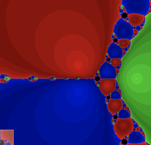
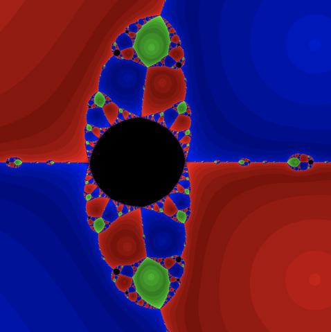
Figure 1. For every degree $d\geq 3$ and every period $m\geq 2$ there is a polynomial $p$ of degree $d$ so that $N_{p}$ has a periodic point of period $m$ that attracts a neighborhood of each of its points. Left: The Newton dynamics plane for $p(Z)=Z^{3}-2Z+2$, where $N_{p}(z)=z-\frac{z^{3}-2z+2}{3z^{2}-2}=\frac{2z^{3}-2}{3z^{2}-2}$ has an attracting $2$-cycle $0\mapsto 1\mapsto 0$; its basin is shown in black. Right: Detail near center.

Newton’s method for polynomials of degree $1$ is trivial: the Newton map is the constant map with value at the root. For degree $2$, the dynamics is very simple as well; we note this here for later use.

Lemma 2.3 (Newton’s method for quadratic polynomials).

If $p$ is a polynomial of degree $2$ with distinct roots, then $N_{p}$ is conformally conjugate to the squaring map $z\mapsto z^{2}$ on the Riemann sphere. In particular, $N_{p}$ has periodic orbits of each exact period at least $2$, none of which are attracting.

Proof.

By Lemma 2.1, we can take $p(Z)=Z^{2}-1$. Then

$$N_{p}(z)=\frac{z^{2}+1}{2z}=T^{-1}\bigl{(}T(z)^{2}\bigr{)}\quad\text{with}\quad T(z)=\frac{z+1}{z-1}\,.$$

Now fix $n$ and let $\omega$ be a primitive $(2^{n}-1)$-th root of unity. Then $\omega$ has exact order $n$ under the squaring map, so $T^{-1}(\omega)$ has exact order $n$ under $N_{p}$. The multiplier of $\omega$ as a point of order $n$ is $2^{n}$, and this is the same as the multiplier of $T^{-1}(\omega)$ under $N_{p}$. ∎

For completeness, we might note that the Newton map for a quadratic polynomial with a double root is conformally conjugate to $z\mapsto z/2$.

Positive results about Newton’s method

Meanwhile, there is a substantial body of knowledge about the global dynamics of Newton’s method, in stark contrast to the Weierstrass method. Here we mention some of the relevant results.

For the Newton dynamics $N_{p}$, any particular orbit may or may not converge to a root. However, one can estimate that asymptotically at least a fraction of $1/(2\log 2)\approx 0.72$ of randomly chosen points in ${\mathbb{C}}$ will converge to some root (see [HSS]*Section 4). More explicitly, for every degree $d$ there is a universal set $S_{d}$ of starting points that will find, for every polynomial $p$ of degree $d$, normalized so that all roots are in the unit disk, all the roots of $p$ under iteration of $N_{p}$. This set is universal in the sense that it depends only on $d$, and it may have cardinality as low as $1.1d(\log d)^{2}$ [HSS]. If one accepts probabilistic results, then $cd(\log\log d)^{2}$ starting points are sufficient to find all roots with given probability, where $c$ depends only on this probability [BLS]. Upper bounds on the complexity of Newton’s method to find all roots with prescribed precision $\varepsilon$ were established in [NewtonEfficient, BAS]; they can be as good as $O(d^{2}(\log d)^{4}+d\log|\log\varepsilon|)$, which is close to optimal when the starting points are outside of a disk containing the roots.

In addition to these strong theoretical results, Newton’s method has also been used successfully in practice for finding all roots of polynomials of degrees exceeding $10^{9}$ [NewtonRobin1, NewtonRobin2], and it is interesting to compare the experimental complexity between the Newton and Ehrlich–Aberth methods; see [NewtonExperiments]: depending on the efficiency how the polynomials can be evaluated, and how the roots are located, one or the other method may be faster.

Finally, we might mention that there are several other complex one-dimensional root finding iteration methods, including König’s method; see [XavierChristianRootFinders]. However, there is a theorem by McMullen [McMullenRootFinding] that no one-dimensional root finding method can be generally convergent. It is natural to ask whether a similar result holds also for root finding methods in several variables.

3   The Weierstrass method

The Weierstrass root finding method, also known as the Durand–Kerner method, tries to approximate all $d$ roots of a degree $d$ polynomial simultaneously (unlike the Newton method, which approximates only one root at a time). Recall that ${\mathcal{P}}^{\prime}_{d}$ is the space of monic polynomials of degree $d$. Let $p\in{\mathcal{P}}^{\prime}_{d}$. Then the Weierstrass root finding method consists of iterating the (partially defined) map $W_{p}\colon{\mathbb{C}}^{d}\to{\mathbb{C}}^{d}$, $\underline{z}\mapsto\underline{z}^{\prime}$, where the components $z^{\prime}_{k}$ of $\underline{z}^{\prime}$ are given in terms of those of $\underline{z}$ by

(3.1) $$z^{\prime}_{k}=z_{k}-\frac{p(z_{k})}{\prod_{j\neq k}(z_{k}-z_{j})}\,.$$

This map is defined for all $\underline{z}\in{\mathbb{C}}^{d}\setminus\Delta$, where $\Delta$ is the “big diagonal”

$$\Delta=\{\underline{z}\in{\mathbb{C}}^{d}:\text{$z_{j}=z_{k}$ for some $1\leq j<k\leq d$}\}\,.$$

If $p$ is not necessarily monic, then $W_{p}$ is defined to be the same as $W_{p/c}$, where $c$ is the leading coefficient of $p$. It is therefore sufficient to consider only monic polynomials.

The Weierstrass method converges on a non-empty open subset of ${\mathbb{C}}^{d}$ to a vector containing the $d$ roots in some order. It is well known that iteration of $W_{p}$ may land on $\Delta$ after any number of steps even when the starting point $\underline{z}$ is not in $\Delta$. Moreover, even when an orbit is defined forever it may fail to converge to roots: for instance, when a polynomial is real but its roots are not, then a vector of purely real initial points cannot converge to non-real solutions; similar arguments apply in the presence of other symmetries. More generally, different vectors of starting points may converge to the roots in different order, and the respective domains of convergence in ${\mathbb{C}}^{d}$ must have non-empty boundaries on which convergence cannot occur. The best possible outcome to hope for would be that convergence to roots occurs on an open dense subset of ${\mathbb{C}}^{d}$, ideally with complement of measure zero.

Obviously, if $z_{k}$ is already a root, then the map has a fixed point in the $k$-th coordinate; all roots already found stabilize in the approximation vector (as long as they are all distinct).

One heuristic interpretation of the Weierstrass method is as follows. Each of the $d$ component variables “thinks” that all other roots have already been found and tries to find its own value necessary to match the value of the polynomial at a single point. To make this precise, write again $p(Z)=\prod_{k}(Z-\alpha_{k})$. Take a coordinate $k\in\{1,\dots,d\}$; if we assume that $z_{j}=\alpha_{j}$ for all $j\neq k$, then

(3.2) $$p(z_{k})=(z_{k}-\alpha_{k})\prod_{j\neq k}(z_{k}-z_{j})\,,$$

and then the method simply “finds” the missing root $\alpha_{k}$ as the only unknown quantity in (3.2) to make the equation fit. This leads to the Weierstrass iteration formula (3.1). For the Weierstrass method, all $k$ variables make the same “assumption” and in general they are all wrong, but it turns out anyway that this leads to a reasonable approximation of the root vectors, at least sufficiently close to a true solution.

We will now show that the Weierstrass method can be interpreted as a higher-dimensional Newton iteration. Consider the map

$$F\colon{\mathbb{C}}^{d}\longrightarrow{\mathcal{P}}^{\prime}_{d}\,,\qquad(z_{1},\dots,z_{d})\longmapsto\prod_{k=1}^{d}(Z-z_{k})\,.$$

Then the task of finding all the roots of $p$ is equivalent to finding some preimage of $p$ under $F$. To solve this problem, we can employ Newton’s method in $d$ dimensions. This leads to the iteration

(3.3) $$\underline{z}\longmapsto\underline{z}-(\mathbf{D}(F)_{|\underline{z}})^{-1}(F(\underline{z})-p)\,,$$

which is defined on the set of $\underline{z}\in{\mathbb{C}}^{d}$ where $\mathbf{D}(F)_{|\underline{z}}$ is invertible, which is the case if and only if $\underline{z}\notin\Delta$. (The “if” direction follows from the proof below; the “only if” direction is easy.)

Lemma 3.1 (Weierstrass method as higher-dimensional Newton).

The map given by (3.3) is $W_{p}$.

Proof.

First note that the partial derivative of $F$ with respect to the $k$-th coordinate $z_{k}$ is

$$\frac{\partial F}{\partial z_{k}}(\underline{z})=-\prod_{j\neq k}(Z-z_{j})\,,$$

where the expression on the right is a polynomial of degree less than $d$; we identify the space of such polynomials with ${\mathbb{C}}^{d}$. If we denote the right hand side of (3.3) by $\underline{z}^{\prime}$, we can write (3.3) in the form

(3.4) $$\mathbf{D}(F)_{|\underline{z}}(\underline{z}^{\prime}-\underline{z})=p-F(\underline{z})\,.$$

Written out, this gives

(3.5) $$\sum_{k=1}^{d}(z^{\prime}_{k}-z_{k})\prod_{j\neq k}(Z-z_{j})=\prod_{k=1}^{d}(Z-z_{k})-p\,.$$

If we assume that the entries of $\underline{z}$ are distinct and, separately for each $m\in\{1,\ldots,d\}$, we set $Z\leftarrow z_{m}$, the product on the right and most products on the left vanish and the remaining equation gives (3.1) (with $m$ in place of $k$). ∎

The following local convergence result is well known.

Lemma 3.2 (Local convergence of the Weierstrass method).

Every vector consisting of the $d$ roots of $p$ has a neighborhood in ${\mathbb{C}}^{d}$ on which the Weierstrass method converges to this solution vector. This convergence is quadratic when $p$ has no multiple roots.

Proof.

This follows from the fact that $W_{p}$ is Newton’s method applied to $F(\underline{z})-p$. ∎

3.1   Properties of the Weierstrass method

We state some elementary and well known properties of $W_{p}$ that will be important to us.

Lemma 3.3 (Simple properties of the Weierstrass method).

1. Let $p\in{\mathcal{P}}^{\prime}_{d}$ and $T\in\operatorname{Aff}({\mathbb{C}})$. Then $W_{Tp}$ is is conformally conjugate to $W_{p}$ by $T$, i.e., $W_{Tp}=T\circ W_{p}\circ T^{-1}$, where the action of $T$ on ${\mathbb{C}}^{d}$ is component-wise.

2. For each $p\in{\mathcal{P}}^{\prime}_{d}$, $W_{p}$ is equivariant with respect to the natural action of the symmetric group$~{}S_{d}$ on on ${\mathbb{C}}^{d}$ by permuting the coordinates: if $\sigma\in S_{d}$, then $W_{p}(\sigma\underline{z})=\sigma W_{p}(\underline{z})$.

Proof.

1. Writing $p=\prod_{k=1}^{d}(Z-\alpha_{k})$ in (3.5), we see that the relation is unchanged when we replace $\alpha_{k}$, $z_{k}$, $z^{\prime}_{k}$ and $Z$ by their images under $T$. Undoing the transformation on $Z$ then gives a valid equation between polynomials, which is equivalent to $W_{Tp}(T\underline{z})=TW_{p}(\underline{z})$, or $W_{Tp}=T\circ W_{p}\circ T^{-1}$, where the action of affine transformations on ${\mathbb{C}}^{d}$ is coordinate-wise.

2. This is clear. ∎

By the first property we can use the same parameter space ${\mathcal{P}}_{d}$ for the Weierstrass iteration on polynomials of degree $d$ as we did for Newton’s method.

Equation (3.5) leads to a simple proof of the following useful property.

Lemma 3.4 (Invariant hyperplane).

Let $p=Z^{d}-aZ^{d-1}+\ldots$. Then the sum of the entries of $W_{p}(\underline{z})$ is $a$, for all $\underline{z}\in{\mathbb{C}}^{d}\setminus\Delta$.

Proof.

Comparing coefficients of $Z^{d-1}$ in (3.5), we see that

$$\sum_{k=1}^{d}(z^{\prime}_{k}-z_{k})=-\sum_{k=1}^{d}z_{k}+a\,,$$

which gives the claim. ∎

This means that the dynamics is effectively only $(d-1)$-dimensional and takes place on the hyperplane $z_{1}+\ldots+z_{d}=a$. As mentioned earlier, we can restrict to centered polynomials, i.e., $a=0$.

Lemma 3.5 (Degree reduction if root is present).

Fix $k\in\{1,\ldots,d\}$. If $z_{k}$ is a root of $p$ and $\underline{z}\in{\mathbb{C}}^{d}\setminus\Delta$, then $W_{p}(\underline{z})_{k}=z_{k}$, and the dynamics on the remaining entries is that of the Weierstrass method for $p(Z)/(Z-z_{k})$.

Proof.

Clear from the definition. ∎

Lemma 3.6 (Weierstrass in degree $2$ is Newton).

If $p$ has degree $2$, then the dynamics of $W_{p}$ reduces to Newton’s method for $p$. In particular, for $p$ with distinct roots, $W_{p}$ restricted to the invariant hyperplane (which is a line in this case) is conjugate to the squaring map $z\mapsto z^{2}$, which has no attracting cycles that are not fixed points.

Proof.

By Lemma 3.3, we can assume that $p(Z)=Z^{2}-1$ if $p$ has distinct roots. By Lemma 3.4, all iterates after the initial vector will have the form $(z,-z)$. It is then easy to check that $W_{p}(z,-z)=(w,-w)$ with $w=z-(z^{2}-1)/(2z)=N_{p}(z)$. The last claim follows from Lemma 2.3.

If $p$ has a double root, then $N_{p}$ and $W_{p}$ are conjugate to $N_{Z^{2}}$ and $W_{Z^{2}}$, respectively; again, $W_{Z^{2}}$ agrees with $N_{Z^{2}}$ when restricted to the invariant line. ∎

When $p$ is linear, then $N_{p}$ and $W_{p}$ both find the unique root immediately by definition. So this lemma tells us that interesting behavior in the Weierstrass method can occur only when $d\geq 3$.

When looking for periodic orbits under $W_{p}$, Lemma 3.5 tells us that we can assume that no entry of $\underline{z}$ is a root of $p$, since otherwise we can reduce to a case of lower degree. However, this very observation allows us to promote counterexamples of low degrees to higher degrees. To do this, we need the following lemma.

Lemma 3.7 (Lifting to higher degrees).

Let $p$ be a monic polynomial of degree $d$ and let $\alpha\in{\mathbb{C}}$. Set $\tilde{p}(Z)=(Z-\alpha)p(Z)$.

1. For a point $\underline{z}=(z_{1},\ldots,z_{d},\alpha)$ with pairwise distinct entries, the Jacobi matrix $\mathbf{D}(W_{\tilde{p}})_{|\underline{z}}$ has the form

   $$\mathbf{D}(W_{\tilde{p}})_{|\underline{z}}=\begin{pmatrix}\mathbf{D}(W_{p})_{|\underline{z}^{\prime}}&*_{d\times 1}\\ 0_{1\times d}&\lambda\end{pmatrix}$$

   with $\underline{z}^{\prime}=(z_{1},\ldots,z_{d})$ and

   $$\lambda=1-\frac{p(\alpha)}{\prod_{j=1}^{d}(\alpha-z_{j})}\,.$$

2. If $q\in{\mathbb{C}}^{d}$ is a periodic point of $W_{p}$ of period $n$ such that all eigenvalues of $\mathbf{D}(W_{p}^{\circ n})_{|q}$ have absolute values strictly less than $1$, then for $|\alpha|$ sufficiently large, $\tilde{q}:=(q,\alpha)\in{\mathbb{C}}^{d+1}$ is a periodic point of $W_{\tilde{p}}$ of period $n$ such that all eigenvalues of $\mathbf{D}(W_{\tilde{p}}^{\circ n})_{|\tilde{q}}$ have absolute values strictly less than $1$.

Proof.

The first claim results from an easy computation.

Now assume that $q\in{\mathbb{C}}^{d}$ is a periodic point of $W_{p}$ of period $n$. By Lemma 3.5, $\tilde{q}=(q,\alpha)$ is a periodic point of $W_{\tilde{p}}$ of period $n$. We obtain an analogous formula relating the derivatives of $W_{p}^{\circ n}$ at $q$ and $W_{\tilde{p}}^{\circ n}$ at $\tilde{q}$, with the product $\lambda_{0}\cdots\lambda_{n-1}$ replacing $\lambda$, where $\lambda_{m}$ arises from $(W_{p}^{\circ m}(q),\alpha)$. In particular, the eigenvalues of $\mathbf{D}(W_{\tilde{p}}^{\circ n})_{|\tilde{q}}$ are those of $\mathbf{D}(W_{p}^{\circ n})_{|q}$ together with $\lambda_{0}\cdots\lambda_{n-1}$. As $|\alpha|\to\infty$, we see that $\lambda_{m}\to 0$ for all $0\leq m<n$, and the claim follows. ∎

3.2   The dynamics of $W_{Z^{3}}$

In this section we prove some results on the dynamics of the Weierstrass iteration in the simple case when $p(Z)=Z^{3}$. By Lemma 3.4, we can restrict consideration to the hyperplane $H=\{z_{1}+z_{2}+z_{3}=0\}$. We will show that all starting points in $H$ outside a set of measure zero converge to the unique root vector $(0,0,0)$, but that there are uncountably many orbits that converge to infinity.

From Lemma 3.3 (1) and since the unique root $0$ of $Z^{3}$ is invariant under scaling, it follows that $W_{Z^{3}}(\lambda\underline{z})=\lambda W_{Z^{3}}(\underline{z})$, so $W_{Z^{3}}$ induces a rational map $\varphi\colon{\mathbb{P}}H\to{\mathbb{P}}H$, where ${\mathbb{P}}H\simeq{\mathbb{P}}^{1}$ is the complex projective line obtained by considering the nonzero points of $H$ up to scaling.

Writing a nonzero point in $H$ up to scaling in the form $(1,z,-1-z)$ (the missing scalar multiples of $(0,1,-1)$ correspond to the limit case $z=\infty$), we find that

(3.6) $$W_{Z^{3}}(1,z,-1-z)=s(z)(1,\varphi(z),-1-\varphi(z))$$

with

(3.7) $$s(z)=\frac{1-z-z^{2}}{2-z-z^{2}}\qquad\text{and}\qquad\varphi(z)=\frac{z(2+z)(1+z-z^{2})}{(1+2z)(1-z-z^{2})}\,.$$

We can say something about the dynamics of $\varphi$.

Lemma 3.8 (Dynamics of $\varphi$).

The map $\varphi$ has two attracting fixed points at $\omega$ and $\omega^{2}$, where $\omega=e^{2\pi i/3}$ is a primitive cube root of unity. Let $z\in{\mathbb{C}}$. If $\operatorname{Im}(z)>0$, then $\varphi^{\circ n}(z)$ converges to $\omega$ as $n\to\infty$, and if $\operatorname{Im}(z)<0$, then $\varphi^{\circ n}(z)$ converges to $\omega^{2}$ as $n\to\infty$. The real line is forward and backward invariant under $\varphi$.

Proof.

Conjugating $\varphi$ by the Möbius transformation $z\mapsto(\omega^{2}z-\omega^{2})/(z-\omega)$, we obtain

$$f(z)=z\frac{2z^{3}+1}{z^{3}+2}\,.$$

This map $f$ is the product of $z$ with the composition of $z\mapsto z^{3}$ by $z\mapsto(2z+1)/(z+2)$; the latter is an automorphism of the open unit disk (and also of the complement of the closed unit disk in the Riemann sphere). Therefore, $|f(z)|<|z|$ when $0<|z|<1$ and $|f(z)|>|z|$ for $|z|>1$ (in other words, $f$ is a Blaschke product with a fixed point at $z=0$). This implies that the open unit disk is attracted to the fixed point $0$ of $f$, while the complement of the closed unit disk is attracted to $\infty$; the unit circle is forward and backward invariant (and maps to itself as a covering map with degree $4$). Translating back to $\varphi$, this gives the result. ∎

From this, we can deduce the following statement on the global dynamics of $W_{Z^{3}}$.

Theorem 3.9 (Convergence of $W_{Z^{3}}$).

If $\underline{z}\in H$ is not a scalar multiple of a vector with real entries, then $W_{Z^{3}}^{\circ n}(\underline{z})$ converges to the zero vector. The convergence is linear with rate of convergence $2/3$.

Note that the rate of convergence is the same as that for $N_{Z^{3}}$.

Proof.

Let $\underline{z}\in H$ be such that $\underline{z}$ is not a scalar multiple of a vector with real entries. In particular, $\underline{z}$ is not the zero vector. By symmetry, we can assume that the first entry is nonzero; then $\underline{z}=z_{1}(1,z,-1-z)$ with $z=z_{2}/z_{1}\in{\mathbb{C}}\setminus{\mathbb{R}}$. We then have that $\varphi^{\circ n}(z)\neq\infty$ for all $n\geq 0$ by Lemma 3.8, and

$$W_{Z^{3}}^{\circ n}(\underline{z})=\prod_{k=0}^{n-1}s(\varphi^{\circ k}(z))\cdot(1,\varphi^{\circ n}(z),-1-\varphi^{\circ n}(z))\,.$$

By Lemma 3.8 again, $\varphi^{\circ n}(z)$ converges to $\omega$ or $\omega^{2}$. Since $s(\omega)=s(\omega^{2})=2/3$, the factor in front will linearly converge to zero with rate of convergence $2/3$, whereas the vector will converge to $(1,\omega,\omega^{2})$ (if $\operatorname{Im}(z)>0$) or to $(1,\omega^{2},\omega)$ (if $\operatorname{Im}(z)<0$). ∎

We have seen that orbits of starting points in $H$ that are not scalar multiples of real vectors converge to zero, whereas there are real vectors in $H$ whose orbit tends to infinity; see Section 3.3 below. There are also starting points whose orbits cease to be defined after finitely many steps; this occurs if and only if some iterate is a multiple of $(1,1-2)$ or one of its permutations. On the other hand, there are many real starting points in $H$ whose orbits tend to zero (one example is obtained by replacing $\alpha$ with $-\alpha$ in the proof of Theorem 3.10 below). In fact, we expect that almost all real starting points have this property.

3.3   Escaping points

In this section we prove Theorem B: the Weierstrass iteration $W_{p}$ has escaping points for all polynomials of degree $d\geq 3$ with distinct roots.

We first continue our study of the cubic case, $d=3$. As observed earlier, we can always assume that our polynomial $p$ is centered, i.e., has the form $p=Z^{3}+aZ+b$. Then the image of $W_{p}$ is contained in the plane $H=\{z_{1}+z_{2}+z_{3}=0\}$, so it is sufficient to consider the induced map $H\to H$. We identify $H$ with ${\mathbb{C}}^{2}$ by projecting to the first two coordinates. We can then extend $W_{p}$ to a rational map ${\mathbb{P}}^{2}\to{\mathbb{P}}^{2}$, which is given by the following triple of quartic polynomials, as a simple computation shows.

$$(z_{1}:z_{2}:z_{0})\longmapsto\bigl{(} (z_{1}+2z_{2})(z_{1}^{3}+az_{1}z_{0}^{2}+bz_{0}^{3}-z_{1}z_{2}(z_{1}+z_{2}))$$

(3.8) $${}:(2z_{1}+z_{2})(-z_{2}^{3}-az_{2}z_{0}^{2}-bz_{0}^{3}+z_{1}z_{2}(z_{1}+z_{2}))$$

$${}:z_{0}(z_{1}-z_{2})(z_{1}+2z_{2})(2z_{1}+z_{2})\bigr{)}$$

Here the line at infinity is given by $z_{0}=0$; it is forward invariant, and the induced dynamics on this projective line is given by the rational map $\varphi$ from Section 3.2.

Theorem 3.10 (Escaping orbits for cubic polynomials).

For every cubic polynomial $p$, there are starting points $\underline{z}\in{\mathbb{C}}^{3}$ such that the iteration sequence $(W_{p}^{\circ n}(\underline{z}))$ exists for all times and converges component-wise to infinity. The set of escaping points contains a holomorphic curve.

Proof.

Let

$$\alpha=-\sqrt{\frac{5+\sqrt{21}}{2}}\,.$$

Then one can check that the point $q_{0}=(1:\alpha:0)$ on the line at infinity is $2$-periodic for the extension of $W_{p}$ to ${\mathbb{P}}^{2}$. We consider $q_{0}$ as a fixed point of the second iterate of this extension. Its multiplier matrix has eigenvalues

$$12\alpha^{3}-72\alpha+43=43+12\sqrt{7}>1\quad\text{and}\quad\frac{-\alpha^{3}+6\alpha+4}{2}=2-\tfrac{1}{2}\sqrt{7}\in(0,1)\,.$$

The eigenspace for the first of these eigenvalues is tangential to the line at infinity, whereas the eigenspace for the second eigenvalue points away from the line. So the point $q_{0}$ has a stable manifold (see [Palis-deMelo]*Ch. 2, Section 6 for the general theory) that meets the (complex) line at infinity locally only at $q_{0}$ and is a holomorphic curve by [Hubbard2005]*Cor. 8. In particular, all points $q\in H$ that lie on the stable manifold and are sufficiently close to $q_{0}$ will converge in ${\mathbb{P}}^{2}$ to the $2$-cycle that $q_{0}$ is part of. Since the points of this $2$-cycle are on the line at infinity (and different from $(1:0:0)$, $(0:1:0)$, $(1:-1:0)$, which are the points corresponding to the lines $z_{1}=0$, $z_{2}=0$ and $z_{3}=-z_{1}-z_{2}=0$), the claim follows. ∎

Remark 3.11.

When $p=Z^{3}$, the stable manifold of $q_{0}$ is the complex line joining it to $(0:0:1)$. So in this case, every scalar multiple of $(1,\alpha,-1-\alpha)\in H$ escapes to infinity.

Now Theorem B follows from Theorem 3.10 in the following way. Write $p=p_{1}p_{2}$ with $p_{1}$ of degree $3$ and $p_{2}$ with simple roots. By Theorem 3.10 there is a vector $q_{1}\in{\mathbb{C}}^{3}$ that escapes to infinity under $W_{p_{1}}$. Now set $q=(q_{1},q_{2})$, where $q_{2}\in{\mathbb{C}}^{d-3}$ has the roots of $p_{2}$ (in some order) as entries. Then iterating $W_{p}$ on $q$ has the effect of fixing the last $d-3$ coordinates, whereas the effect on the first three is that of $W_{p_{1}}$; see Lemma 3.5. In particular, the first three coordinates of the vectors in the orbit of $q$ under $W_{p}$ tend to infinity. Note that this result covers a slightly larger set of polynomials than those with simple roots: the cubic factor $p_{1}$ is arbitrary, so $p$ can have a multiple root of order at most $4$ or two double roots.

Taking iterated preimages under $W_{p}$ of the curve to infinity whose existence we have shown in Theorem 3.10 above, we obtain countably infinitely many (complex) curves to infinity full of escaping points. Here we restrict to iterated preimage curves ending in an iterated preimage of the point $q_{0}$ (notation as in the proof above) that is on the line at infinity. Two of the immediate preimage curves end at the origin, which is a point of indeterminacy for the rational map (3.8) induced by $W_{p}$. There are very likely other escaping points, but we expect the set of escaping points to be of measure zero within $H$.

4   Algebraic description of periodic orbits

Since we will be using methods from Computer Algebra to obtain a proof of the Theorem A, we now discuss how we can describe the periodic points of $W_{p}$ of any given period algebraically. We begin with a description of $W_{p}$ itself.

4.1   Algebraic description of $W_{p}$

For the purpose of studying periodic orbits under $W_{p}$ algebraically as $p$ varies, equation (3.5) is preferable to (3.1), since it is a polynomial equation involving the entries of $\underline{z}$ and $\underline{z}^{\prime}$ and the coefficients of $p$, rather than an equation involving rational functions. The following result shows that we do not get extraneous solutions by doing so, in the sense that all solutions we find that involve points in $\Delta$ arise as degenerations of “honest” solutions living outside $\Delta$.

Proposition 4.1 (Polynomial equation describing iteration).

Fix $p\in{\mathcal{P}}^{\prime}_{d}$. The algebraic variety in ${\mathbb{C}}^{d}\times{\mathbb{C}}^{d}$ described by equation (3.5) is the Zariski closure of the graph of $W_{p}$ (which is contained in $({\mathbb{C}}^{d}\setminus\Delta)\times{\mathbb{C}}^{d}$).

Proof.

Let $V_{p}$ denote the variety in question. Equation (3.5) corresponds to $d$ equations in the $2d$ coordinates of $\underline{z}$ and $\underline{z}^{\prime}$, so each irreducible component of $V_{p}$ must have dimension at least $d$. We have to show that no irreducible component is contained in $\Delta\times{\mathbb{C}}^{d}$. We do this by showing that $\dim(V_{p}\cap(\Delta\times{\mathbb{C}}^{d}))<d$.

Assume that $\underline{z}\in\Delta$. We first consider the simplest case that $z_{1}=z_{2}$, but $z_{2},\ldots,z_{d}$ are distinct. Substituting $Z\leftarrow z_{1}$ in (3.5), we obtain that $p(z_{1})=0$, so that $z_{1}$ must be a root of $p$. The subset of $\Delta$ consisting of $\underline{z}$ with this property has dimension $d-2$. Substituting $Z\leftarrow z_{k}$ with $k\geq 3$, we see that $z^{\prime}_{k}$ is uniquely determined by $\underline{z}$ (it is still given by (3.1)). On the other hand, taking the derivative with respect to $Z$ on both sides and then substituting $Z\leftarrow z_{1}$, we see that $z^{\prime}_{1}+z^{\prime}_{2}$ is uniquely determined, so the fiber above $\underline{z}$ of the projection of $V_{p}$ to the first factor has dimension $1$. So the part of $V_{p}\cap(\Delta\times{\mathbb{C}}^{d})$ lying above points $\underline{z}$ with only one double entry has dimension $d-1$.

In general, we see by similar considerations (taking higher derivatives as necessary) that when $\underline{z}$ has entries of multiplicities $m_{1},\ldots,m_{l}$ (with $m_{1}+\ldots+m_{l}=d$ and some $m_{j}\geq 2$), then these entries must be roots of $p$ of multiplicities (at least) $m_{1}-1,\ldots,m_{l}-1$, and the fiber of $V_{p}$ above $\underline{z}$ is a linear space of dimension $(m_{1}-1)+\ldots+(m_{l}-1)=d-l$. On the other hand, the set of $\underline{z}$ of this type has dimension $\#\{j:m_{j}=1\}<l$, so the dimension of the corresponding subset of $V_{p}$ is $<d$.

So we have seen that $V_{p}\cap(\Delta\times{\mathbb{C}}^{d})$ is a finite union of algebraic sets of dimension $<d$; therefore it cannot contain an irreducible component of $V_{p}$. ∎

Remark 4.2.

As in the proof above, we will usually think of (3.5) as a system of $d$ equations that are obtained by comparing the coefficients of the various powers of $Z$ on both sides. Note that the equation for the coefficient of $Z^{j}$ is of degree $d-j$ in $z_{1},\dots,z_{d},z_{1}^{\prime},\dots,z_{d}^{\prime}$. So the total system has degree $d!$.

4.2   Periodic points

We use equation (3.5) to obtain a system of equations representing periodic points. Fix the degree $d$ and the period $n$. We consider $nd$ variables, grouped into $n$ vectors $\underline{z}^{(k)}=(z_{1}^{(k)},\ldots,z_{d}^{(k)})$, for $0\leq k<n$, which we think of as representing an $n$-cycle $\underline{z}^{(0)}$, $\underline{z}^{(1)}=W_{p}(\underline{z}^{(0)})$, …, $\underline{z}^{(n-1)}=W_{p}(\underline{z}^{(n-2)})$, $\underline{z}^{(0)}=W_{p}(\underline{z}^{(n-1)})$. We therefore define the scheme ${\mathcal{P}}^{\prime}_{d}(n)\subset{\mathcal{P}}^{\prime}_{d}\times{\mathbb{C}}^{nd}$ by collecting the equations arising from comparing coefficients on both sides of (3.5), where we replace $(\underline{z},\underline{z}^{\prime})$ successively by $(\underline{z}^{(0)},\underline{z}^{(1)})$, $(\underline{z}^{(1)},\underline{z}^{(2)})$, …, $(\underline{z}^{(n-1)},\underline{z}^{(0)})$; $p$ runs through the monic degree $d$ polynomials in ${\mathcal{P}}^{\prime}_{d}$. This encodes that $\underline{z}^{(0)}\mapsto\underline{z}^{(1)}\mapsto\ldots\mapsto\underline{z}^{(n-1)}\mapsto\underline{z}^{(0)}$ under $W_{p}$. We then take ${\mathcal{P}}_{d}(n)$ to be the quotient of ${\mathcal{P}}^{\prime}_{d}(n)$ by the group of affine transformations on ${\mathbb{C}}$, acting via

$$T\cdot(p,z^{(0)}_{1},\ldots,z^{(n-1)}_{d})=(Tp,Tz^{(0)}_{1},\ldots,Tz^{(n-1)}_{d})\,.$$

We expect the fibers of the projection ${\mathcal{P}}_{d}(n)\to{\mathcal{P}}_{d}$ to be finite, i.e., that for each polynomial $p$, there are only finitely many points of period $n$ under $W_{p}$. The following lemma gives a criterion for when this is the case.

Lemma 4.3 (Criterion for finiteness of $n$-periodic points).

Let ${\mathcal{P}}_{d}^{(0)}(n)\subset{\mathbb{C}}^{nd}$ be the fiber of ${\mathcal{P}}^{\prime}_{d}(n)$ above $p=Z^{d}$. The projection ${\mathcal{P}}^{\prime}_{d}(n)\to{\mathcal{P}}^{\prime}_{d}$ is finite if and only if ${\mathcal{P}}_{d}^{(0)}(n)=\{0\}$.

Proof.

We first note that since the unique root $0$ of $Z^{d}$ is fixed by scaling, the same is true for ${\mathcal{P}}_{d}^{(0)}(n)$ under simultaneous scaling of the coordinates. So ${\mathcal{P}}_{d}^{(0)}(n)=\{0\}$ is equivalent to ${\mathcal{P}}_{d}^{(0)}(n)$ being zero-dimensional. In particular, if ${\mathcal{P}}_{d}^{(0)}(n)\neq\{0\}$, then the projection is not finite, since the fiber above $Z^{d}$ has positive dimension. This proves one direction of the claimed equivalence.

Now assume that the projection is not finite, so there is some $p\in{\mathcal{P}}_{d}$ such that the fiber ${\mathcal{P}}_{d}^{(p)}(n)$ above $p$ has positive dimension. Let $\bar{{\mathcal{P}}}_{d}^{(p)}(n)\subset{\mathbb{P}}^{nd}$ denote the projective scheme obtained by homogenizing the equations defining ${\mathcal{P}}^{\prime}_{d}(n)$ and specializing to $p$. Then ${\mathcal{P}}_{d}^{(p)}(n)$ meets the hyperplane at infinity of ${\mathbb{P}}^{nd}$. But the intersection of ${\mathcal{P}}_{d}^{(p)}(n)$ with the hyperplane at infinity is exactly the image of ${\mathcal{P}}_{d}^{(0)}(n)$ under the projection ${\mathbb{C}}^{nd}\setminus\{0\}\to{\mathbb{P}}^{nd-1}$. So this image is non-empty, which implies that ${\mathcal{P}}_{d}^{(0)}(n)$ contains non-zero points. This shows the other direction. ∎

We can test the condition “${\mathcal{P}}_{d}^{(0)}(n)=\{0\}$” with a Computer Algebra System by setting up the ideal that is generated by the equations defining ${\mathcal{P}}_{d}^{(0)}(n)$, together with $z^{(0)}_{1}-1$ (for symmetry reasons, if there is some nonzero point, then there is one with $z^{(0)}_{1}\neq 0$, and by scaling, we can assume that $z^{(0)}_{1}=1$). Then we compute a Groebner basis for this ideal. The condition is satisfied if and only if this Groebner basis contains $1$. We did this for $d=3$ and small values of $n$.

Lemma 4.4 (Finiteness of $n$-periodic points).

For every cubic polynomial $p$ with at least two distinct roots, there are only finitely many points of period $n\leq 8$ under $W_{p}$. For cubic polynomials with a triple root, the statement holds for all $n\leq 8$ except $n=6$.

Proof.

The claim follows for $n\in\{1,2,3,4,5,7,8\}$ from Lemma 4.3 and a computation as described above. For $n=6$, we find that ${\mathcal{P}}_{3}^{(0)}(6)$ consists of six lines through the origin (plus the origin with high multiplicity). These six lines correspond to $6$-cycles of rotation type (see Section 5 below for the definition). By an explicit computation (see also Proposition 5.8), we check that the fiber above any polynomial with at least two distinct roots of the scheme describing $6$-periodic points of rotation type is finite. For the remaining components of ${\mathcal{P}}^{\prime}_{3}(6)$, we find that the corresponding part of ${\mathcal{P}}_{3}^{(0)}(6)$ has the origin as its only point; we can then conclude as in the proof of Lemma 4.3 that there are only finitely many $6$-periodic points not of rotation type for all cubic polynomials. ∎

Remark 4.5.

We expect that for cubic polynomials without a triple root, the statement of Lemma 4.4 holds for all $n$. For cubic polynomials with a triple root, we expect that the $6$-periodic points of rotation type are the only exceptions, i.e., that there are no points of exact order $n\geq 2$ except the $6$-periodic points of rotation type described in the proof above.

We do not venture to formulate a conjecture for polynomials of degrees higher than $3$. We did verify the criterion of Lemma 4.3 also for $d=4$ and $n=1,2,3$, however; beyond that, the computations become infeasible.

There is a simple argument that shows that periodic points of any order always exist.

Lemma 4.6 (Existence of periodic points).

Fix a monic polynomial $p$ of degree $d\geq 2$ with distinct roots. Then $W_{p}$ has periodic points of all periods $n\geq 1$.

Proof.

For $n=1$, all the vectors consisting of the roots of $p$ in some order are fixed points. So we fix now some $n\geq 2$. Write $p(Z)=\prod_{j=1}^{d}(Z-\alpha_{j})$. Let $\omega$ be a primitive $(2^{n}-1)$-th root of unity. Then $\omega$ has exact period $n$ under the squaring map $z\mapsto z^{2}$, so by Lemma 3.6, there is a point $(z_{1},z_{2})$ of exact order $n$ for the Weierstrass map associated to $(Z-\alpha_{1})(Z-\alpha_{2})$. By Lemma 3.5, the point

$$\underline{z}=(z_{1},z_{2},\alpha_{3},\ldots,\alpha_{d})$$

then has exact period $n$ under $W_{p}$. ∎

One might ask whether there are always periodic points of all periods that do not fix any coordinate (or even, for which all coordinates have the same period $n$).

We are interested in attracting periodic points, i.e., points $q\in{\mathbb{C}}^{d}$ with the property that there is a period $n\geq 2$ and a neighborhood $U$ of $q$ in ${\mathbb{C}}^{d}$ so that $W_{p}^{\circ mn}(z)\to q$ as $m\to\infty$ for all $z\in U$. Consider the linearization $\mathbf{D}(W_{p}^{\circ n})_{|q}$ of the first return map at the point $q$. We call this the multiplier matrix of $q$. Local fixed point theory relates the topological property of being attracting to an algebraic property of this matrix, as in the following statement, which is a consequence of the fact that a differentiable map is locally well-approximated by its derivative.

Lemma 4.7 (Attracting fixed point).

The fixed point $q$ of a differentiable map $W\colon{\mathbb{C}}^{d}\to{\mathbb{C}}^{d}$ is attracting if all eigenvalues of $\mathbf{D}(W)_{|q}$ have absolute values strictly less than $1$. It cannot be attracting unless all eigenvalues have absolute values at most $1$.

In the context of points of period $n$, we consider $W=W_{p}^{\circ n}$. The lemma then tells us that $q$ can only be attracting when all eigenvalues of its multiplier matrix have absolute value at most $1$. Equivalently, the characteristic polynomial of the multiplier matrix has all its roots in the closed complex unit disk. The set of monic polynomials of degree $d$ with this property forms a compact subset ${\mathcal{A}}_{d}$ of ${\mathcal{P}}^{\prime}_{d}$.

In the following, we will always assume that we pick a representative in the affine equivalence class of the polynomial in question that is centered, i.e., with vanishing sum of roots. Then the dynamics of $W_{p}$ takes place in the linear hyperplane $H$ given by $z_{1}+\ldots+z_{d}=0$, and we get ${\mathcal{P}}_{d}(n)\subset{\mathcal{P}}_{d}\times H^{n}$. We can identify ${\mathcal{P}}_{d}(n)$ with its image in ${\mathcal{P}}_{d}\times H$ obtained by projection to the first two factors, $(p,\underline{z}^{(0)},\ldots,\underline{z}^{(n-1)})\mapsto(p,\underline{z}^{(0)})$. Then the points of ${\mathcal{P}}_{d}(n)$ are represented by pairs $(p,q)$, where $p$ is a centered polynomial and $q\in H$ satisfies $W_{p}^{\circ n}(q)=q$. Since we restrict to $H$, the multiplier matrix of any periodic point $q$ is of size $\dim H=d-1$.

To study whether the $n$-cycles parameterized by ${\mathcal{P}}_{d}(n)$ can be attracting, we would like to associate to each such point $(p,q)$ the $d-1$ eigenvalues of the multiplier matrix of $q$ (the eigenvalues do not change under affine conjugation, so this gives a well-defined map). However, there is no natural order on these eigenvalues. To capture them as an unordered $(d-1)$-tuple, we express the eigenvalues instead through their elementary symmetric functions and hence through the characteristic polynomial of the multiplier matrix. In this way, we obtain an algebraic morphism (and therefore a holomorphic map) $\mu_{d,n}\colon{\mathcal{P}}_{d}(n)\to{\mathcal{P}}^{\prime}_{d-1}$, in much the same way as in the context of Newton’s method. Here we think of ${\mathcal{P}}^{\prime}_{d-1}$ as the space of coefficient vectors of the characteristic polynomials.

Our goal is now to find out if the image of $\mu_{d,n}$ meets ${\mathcal{A}}_{d-1}$, the set of polynomials all of whose roots are in the closed unit disk.

Since we expect that ${\mathcal{P}}_{d}(n)$ is a finite-degree covering of ${\mathcal{P}}_{d}$, it should in particular have dimension $\dim{\mathcal{P}}_{d}=d-2$. This would imply that the image of $\mu_{d,n}$ has dimension at most $d-2$ (and we expect it to be exactly $d-2$), so it is contained in a proper algebraic subvariety of ${\mathcal{P}}^{\prime}_{d-1}$. Each irreducible component of ${\mathcal{P}}_{d}(n)$ will map to an irreducible component of this subvariety. Such a subvariety of codimension at least $1$ does not have to intersect a given bounded subset like ${\mathcal{A}}_{d-1}$. This is a marked difference compared to the situation with Newton’s method, where the corresponding multiplier map is surjective, and so examples of attracting $n$-cycles can easily be found.

So our strategy will be to get as good control as we can on the varieties ${\mathcal{P}}_{d}(n)$ (or suitable components of them), find the Zariski closure $X$ of their image under $\mu_{d,n}$ and then check if $X$ meets ${\mathcal{A}}_{d-1}$. If it does not, then clearly no stable $n$-cycle can exist on the component of ${\mathcal{P}}_{d}(n)$ that we are considering. If it does, then we check that it also meets the open subset of ${\mathcal{A}}_{d-1}$ consisting of polynomials with all roots in the open unit disk; then the intersection will contain a relative open subset of $X$ and so it will contain points in the image and such that the corresponding polynomial $p$ has distinct roots.

5   Cycles for cubic polynomials

We will now restrict consideration to cubic polynomials $p$. Using affine transformations, we can assume that $p(Z)=Z^{3}+Z+t$ with some $t\in{\mathbb{C}}$. This choice of parameterization excludes only (the affine equivalence classes of) $Z^{3}-1$ (which corresponds to $t\to\infty$) and the degenerate case $Z^{3}$. The induced map to the true parameter space ${\mathcal{P}}_{3}$ is a double cover identifying $t$ and $-t$. We will abuse notation slightly in the following by writing ${\mathcal{P}}_{3}(n)$ for what is really the pull-back of the true ${\mathcal{P}}_{3}(n)$ to the $t$-line via the parameterization we use here. As mentioned earlier, for such centered polynomials, the dynamics restricts to the plane $H=\{z_{1}+z_{2}+z_{3}=0\}$.

Let $\sigma_{k}(\underline{z})$ denote the $k$-th elementary symmetric polynomial in the entries of $\underline{z}$. We introduce the quantities

$$w_{2}(\underline{z})=\sigma_{2}(\underline{z})-1\quad\text{and}\quad w_{3}(\underline{z})=\sigma_{3}(\underline{z})+t\,.$$

(We shift by the elementary symmetric polynomials in the roots of $p$ to move the image of the fixed points to $(0,0)$.) The map ${\mathbb{C}}^{3}\supset H\to{\mathbb{C}}^{2}$ given by $(w_{2},w_{3})$ has degree $6$.

By the second property in Lemma 3.3, $W_{p}$ induces a map $\widetilde{W}_{p}$ on (a subset of) ${\mathbb{C}}^{2}$ such that

$$\bigl{(}w_{2}(W_{p}(\underline{z})),w_{3}(W_{p}(\underline{z}))\bigr{)}=\widetilde{W}_{p}\bigl{(}w_{2}(\underline{z}),w_{3}(\underline{z})\bigr{)}$$

for all $\underline{z}\in({\mathbb{C}}^{3}\setminus\Delta)\cap H$.

Lemma 5.1.

$\widetilde{W}_{p}$ is given by

$$\widetilde{W}_{p}(w_{2},w_{3})=\frac{1}{\delta}\bigl{(} w_{2}^{2}+2w_{2}^{3}-3w_{3}^{2}-9tw_{2}w_{3}+w_{2}^{4}+6w_{2}w_{3}^{2},$$

$$4w_{2}w_{3}+3tw_{2}^{2}+4w_{2}^{2}w_{3}+2tw_{2}^{3}-9tw_{3}^{2}+w_{2}^{3}w_{3}+8w_{3}^{3}\bigr{)}\,,$$

where

$$\delta=4(1+w_{2})^{3}+27(t-w_{3})^{2}\,.$$

Proof.

Routine calculation with a Computer Algebra System. ∎

Note that this explicit expression shows the quadratic convergence to $(0,0)$ when $p$ has distinct roots, which is equivalent to $4+27t^{2}\neq 0$.

Now suppose we have an $n$-cycle $(\underline{z}^{(0)},\underline{z}^{(1)},\ldots,\underline{z}^{(n-1)})$ under $W_{p}$. It will be attracting only if all eigenvalues of the multiplier matrix $\mathbf{D}(W_{p}^{\circ n})_{|\underline{z}^{(0)}}$ have absolute value at most $1$. Concretely, we consider the map $\mu_{3,n}\colon{\mathcal{P}}_{3}(n)\to{\mathcal{P}}^{\prime}_{2}$ as discussed in Section 4.2. The characteristic polynomial will have the form $Z^{2}+c_{1}Z+c_{0}$ with $c_{0},c_{1}\in{\mathbb{C}}$, and we know from the discussion in Section 4.2 that $c_{0}$ and $c_{1}$ must satisfy an algebraic relation, i.e., the points $(c_{0},c_{1})$ lie on some plane algebraic curve as we run through all possible characteristic polynomials.

We can also consider the image of this $n$-cycle under $(w_{2},w_{3})$, as the map $\mu_{3,n}$ factors through the $(w_{2},w_{3})$-plane. Assuming that $n$ is the minimal period of the cycle, the image cycle can have minimal period $n$, $n/2$ or $n/3$. The second possibility occurs when $n=2k$ is even and $W_{p}^{\circ k}$ acts as a transposition on the vectors in the cycle. In this case, we say that the cycle is of transposition type. The last possibility occurs when $n=3k$ is divisible by $3$ and $W_{p}^{\circ k}$ acts as a cyclic shift on the vectors in the cycle. In this case, we say that the cycle has rotation type. We can then equivalently look at the characteristic polynomial of $\mathbf{D}(\widetilde{W}_{p}^{\circ n})_{|(w_{2},w_{3})(\underline{z})}$ (or with $k$ in place of $n$ in the transposition or rotation type cases).

We will need a criterion that we can use to show that the two relevant eigenvalues can never simultaneously be in the unit disk, in cases when the relation between $c_{0}$ and $c_{1}$ is somewhat involved. The following lemma provides one such criterion.

Lemma 5.2.

Let $P(\lambda,\mu)\in{\mathbb{C}}[\lambda,\mu]$ be a polynomial. Fix a half-line $\ell$ emanating from the origin and some $N\in{\mathbb{Z}}_{>0}$. Let $B$ be the sum of the absolute values of the coefficients of the two partial derivatives of $P$. If for all $j,k\in\{0,1,\ldots,N-1\}$, the distance from $P(e^{2\pi ij/N},e^{2\pi ik/N})$ to $\ell$ exceeds $\pi B/N$, then $P(\lambda,\mu)=0$ has no solutions in ${\mathbb{C}}^{2}$ with $|\lambda|,|\mu|\leq 1$.

Proof.

We first show that the assumptions imply that the image of $P$ on the torus ${\mathbb{S}}^{1}\times{\mathbb{S}}^{1}$ is contained in the slit plane ${\mathbb{C}}^{2}\setminus\ell$. So consider $(u,v)\in[0,1]^{2}$ and pick $(j,k)\in\{0,\ldots,N\}^{2}$ so that $|u-j/N|,|v-k/N|\leq 1/(2N)$. Note that the sum of the absolute values of the partial derivatives of $(u,v)\mapsto F(u,v):=P(e^{2\pi iu},e^{2\pi iv})$ for $u,v\in{\mathbb{R}}$ is bounded by $2\pi B$. This shows that

$$\bigl{|}P(e^{2\pi iu},e^{2\pi iv})-P(e^{2\pi ij/N},e^{2\pi ik/N})\bigr{|}\leq\frac{1}{2N}\|F_{u}\|_{\infty}+\frac{1}{2N}\|F_{v}\|_{\infty}\leq\frac{1}{2N}\cdot 2\pi B=\pi B/N\,.$$

Since the distance of $P(e^{2\pi ij/N},e^{2\pi ik/N})$ from $\ell$ is by assumption larger than $\pi B/N$, it follows that $P(e^{2\pi iu},e^{2\pi iv})\notin\ell$.

We now assume that there is a solution with $|\lambda|,|\mu|\leq 1$, so that the curve defined by $P$ in ${\mathbb{C}}^{2}$ meets the unit bi-disk. Since the curve is unbounded, by continuity there will be a solution with $|\lambda|=1$ and $|\mu|\leq 1$ or $|\mu|=1$ and $|\lambda|\leq 1$. By symmetry, we can assume the former. By the argument principle, the closed curve $\gamma\colon[0,1]\ni s\mapsto P(\lambda,e^{2\pi is})$ has to pass through the origin or wind around it at least once. However, since the assumptions imply that the image of $\gamma$ is contained in the slit plane ${\mathbb{C}}^{2}\setminus\ell$, which does not contain the origin and is simply connected, we obtain a contradiction. ∎

The general procedure for obtaining the results given below is as follows.

1. Set up equations for the variety ${\mathcal{P}}_{3}(n)$ or parts of it using (3.5).

2. Set up the map $\mu_{3,n}$ as a map to the projective plane given by the coefficients of the characteristic polynomial of the multiplier matrix.

3. Use the Groebner Basis machinery of a Computer Algebra System like Magma [Magma] or Singular [Singular] to find the equation of the image curve.

4. Either find a point on the image curve corresponding to a characteristic polynomial with both roots in the unit disk, or show using Lemma 5.2 that no such points exist.

The available machinery can also be used to obtain additional information on the components of the curves ${\mathcal{P}}_{3}(n)$, for example smoothness or the (geometric) genus.

Since the map $\mu_{3,n}$ is given by fairly involved rational functions when $n$ is not very small, Step 3 above may not necessarily be feasible as stated. In this case, we can instead sample some algebraic points on the variety considered (e.g., by specializing the parameter $t$ to a rational value and then determining the solutions of the resulting zero-dimensional system) and consider their images under $\mu_{3,n}$. Given enough of these image points, we can fit a curve of lowest possible degree through them (this is just linear algebra). We can then check that this curve is correct by constructing a generic point on the original variety and checking that its image lies indeed on the curve.

In the following, we always tacitly assume that the vectors occurring in the cycles do not contain roots of $p$. Those that do can easily be described using Lemmas 3.5 and 3.6.

The computations leading to the results given below have been done using the Magma Computer Algebra System [Magma] and also in many cases independently with Singular [Singular]. A Magma script containing code that verifies most of the claims made is available at [Verification].

5.1   Points of order $2$

We begin by considering $2$-cycles. Note that a $2$-cycle of transposition type fixes one component of the vector, which then must be a root of $p$. Since we have excluded cycles of this form (up to the obvious symmetries, there are three of them, one for each root), no $2$-cycles of transposition type have to be considered.

Proposition 5.3.

The $2$-cycles form a smooth irreducible curve of geometric genus $0$; it maps with degree $12$ to the $t$-line. So for each polynomial, there is (generically) one orbit of $2$-cycles under the natural action of $S_{3}\times C_{2}$, where the first factor permutes the vector entries and the second factor performs a cyclic shift along the cycle. The image in $(t,w_{2},w_{3})$-space is the curve

$$w_{2}=-3\,,\qquad 27t^{2}-45tw_{3}+20w_{3}^{2}-20=0$$

of genus $0$. The characteristic polynomial $X^{2}+c_{1}X+c_{0}$ of the multiplier matrix at a point on this curve satisfies the relation $c_{0}+2c_{1}+6=0$. In particular, no $2$-cycle can be attracting.

Proof.

This follows the method outlined above. Note that when both eigenvalues have absolute values at most $1$, we have $|c_{0}|\leq 1$ and $|c_{1}|\leq 2$. ∎

5.2   Points of order $3$

We begin by considering the $3$-cycles of rotation type. They can be defined by (3.5) together with $(z^{\prime}_{1},z^{\prime}_{2},z^{\prime}_{3})=(z_{2},z_{3},z_{1})$ (for one choice of the cyclic permutation involved). Their images under $(w_{2},w_{3})$ are fixed points of $\widetilde{W}_{p}$.

Proposition 5.4.

The $3$-cycles of rotation type form two smooth irreducible curves (as $t$ varies) of geometric genus $0$, according to which of the possible two cyclic permutations results from the action of $W_{p}$; the map to the $t$-line is of degree $6$ in both cases. The images of both curves in $(t,w_{2},w_{3})$-space agree; the image curve is given by the equations

$$w_{2}=-\frac{3}{2}\,,\qquad 216t^{2}-360tw_{3}+152w_{3}^{2}-1=0\,,$$

describing a curve of genus $0$. The characteristic polynomial of the multiplier matrix at a point on this curve (as a fixed point under $\widetilde{W}_{p}$) has the form $X^{2}+3X+a$ for some $a\in{\mathbb{C}}$. In particular, such a $3$-cycle cannot be attracting.

Proof.

This again follows the procedure outlined above. The characteristic polynomials lie on the curve $c_{1}=3$. So the sum of the eigenvalues is $-3$, hence it is not possible that both eigenvalues are in the closed unit disk. ∎

Now we consider “general” $3$-cycles, i.e., $3$-cycles that are not of rotation type.

Proposition 5.5.

The $3$-cycles that are not of rotation type form two irreducible curves of geometric genus $19$, which each map with degree $72$ to the $t$-line and are interchanged by the action of any transposition in $S_{3}$. Each curve therefore contains $8$ orbits of $3$-cycles under the action of $A_{3}\times C_{3}$, and there are in total $8$ orbits under $S_{3}\times C_{3}$, for each fixed $t$. The coefficients $(c_{0},c_{1})$ of the characteristic polynomial of the multiplier matrix at a point in such a $3$-cycle give a point on a rational curve of degree $12$ that can be parameterized as $(c_{0}(u)/c_{2}(u),c_{1}(u)/c_{2}(u))$, where

$$c_{0}(u) =-9u^{12}-162u^{11}-693u^{10}+1434u^{9}+11958u^{8}-32202u^{7}-182301u^{6}$$

$$\qquad{}+578742u^{5}+2069910u^{4}-919718u^{3}-3065685u^{2}+892254u+264295\,,$$

$$c_{1}(u) =u^{12}+26u^{11}+230u^{10}+693u^{9}-3867u^{8}-5844u^{7}+123074u^{6}$$

$$\qquad{}-38381u^{5}-1320149u^{4}+420552u^{3}+4310940u^{2}-4206447u+1442574\,,$$

$$c_{2}(u) =-9u^{10}-63u^{9}+301u^{8}+1126u^{7}-7693u^{6}-3641u^{5}$$

$$\qquad{}+52375u^{4}+13526u^{3}-104463u^{2}-47919u+20987\,.$$

In particular, no such $3$-cycle can be attracting.

Proof.

The computations get quite a bit more involved, so we give more details here. We work in $7$-dimensional affine space over ${\mathbb{Q}}$ with coordinates $(t,x_{0},y_{0},x_{1},y_{1},x_{2},y_{2})$, where the three vectors in the cycle are $\underline{z}^{(j)}=(x_{j},y_{j},-x_{j}-y_{j})$ for $j=0,1,2$. We first set up the scheme giving the cycle $\underline{z}^{(0)}\mapsto\underline{z}^{(1)}\mapsto\underline{z}^{(2)}\mapsto\underline{z}^{(0)}$ under $W_{p}$. Then we remove the subschemes corresponding to cycles that have a fixed component or to $3$-cycles of rotation type. The resulting scheme is a curve mapping with degree $144$ to the $t$-line. Its projection to the $(x_{2},y_{2})$-plane is a curve of degree $48$, whose defining polynomial factors into two irreducibles of degree $24$ each that are interchanged by $x_{2}\leftrightarrow y_{2}$. Let $Q$ denote one of the factors, considered as a bivariate polynomial. Since the projection is birational, this induces the splitting of the original curve into two components. We could compute the genus by working with the birationally equivalent plane curve given by $Q(x,y)=0$. It has $222$ simple nodes (six of which are defined over ${\mathbb{Q}}(\sqrt{6})$; the remaining $214$ are conjugate) and a pair of conjugate singularities defined over ${\mathbb{Q}}(\sqrt{-3})$ that each contribute $6$ to the difference between arithmetic and geometric genus. We obtain

$$g=\frac{23\cdot 22}{2}-222-2\cdot 6=19$$

as claimed.

This is a case where we had to use the sampling-and-interpolation trick to determine the image curve of $\mu_{3,3}$ on one of the components.

After showing that the image curve has geometric genus $0$ (there is one point of multiplicity $4$ at $(8,-9)$ that gives an adjustment of $8$, and there are $47$ further simple nodes, so we obtain $g=11\cdot 10/2-8-47=0$) and finding some smooth rational points on it, we computed a parameterization modulo some large prime that maps $0,1,\infty$ to three specified rational points and lifted it to ${\mathbb{Q}}$. It is then easy to verify that we indeed obtain a parameterization of the curve over ${\mathbb{Q}}$. We then used Magma’s (fairly new and contributed by the third author) ImproveParametrization command to simplify the resulting parameterization.

Finally, we use Lemma 5.2 to show that there is no attracting $3$-cycle (not of rotation type). We find the polynomial $P(\lambda,\mu)=0$ that gives the relation between the eigenvalues $\lambda$ and $\mu$ (by substituting $(c_{0},c_{1})\leftarrow(\lambda\mu,-(\lambda+\mu))$ in the equation relating the coefficients of the characteristic polynomial) and check that the criterion of Lemma 5.2 is satisfied when $\ell$ is the positive real axis and $N=18$. ∎

5.3   Points of order $4$

Judging by the heavy lifting that was necessary to deal with case of general $3$-cycles, looking at general $n$-cycles with $n\geq 4$ seems too daunting a task to attack with confidence along the lines described here. We can, however, consider cycles with extra symmetries. Here we look at $4$-cycles of transposition type.

Proposition 5.6.

The $4$-cycles of transposition type form three irreducible smooth curves of geometric genus $1$, each of degree $24$ over the $t$-line, that are permuted by a cyclic shift of the coordinates. The characteristic polynomial $X^{2}+c_{1}X+c_{0}$ of the multiplier matrix at any associated point (considered as a point of order $2$ under $\tilde{W}_{p}$) satisfies the relation

$$34c_{0}^{4}c_{1}^{2}+169c_{0}^{3}c_{1}^{3}-675c_{0}^{2}c_{1}^{4}-2997c_{0}c_{1}^{5}-2187c_{1}^{6}+68c_{0}^{5}+984c_{0}^{4}c_{1}+3359c_{0}^{3}c_{1}^{2}$$

$${}-19182c_{0}^{2}c_{1}^{3}-88965c_{0}c_{1}^{4}-91584c_{1}^{5}+4254c_{0}^{4}+29059c_{0}^{3}c_{1}-93688c_{0}^{2}c_{1}^{2}$$

$${}-634050c_{0}c_{1}^{3}-809379c_{1}^{4}+76045c_{0}^{3}+60846c_{0}^{2}c_{1}-725626c_{0}c_{1}^{2}-1171592c_{1}^{3}$$

$${}+487003c_{0}^{2}+4167623c_{0}c_{1}+8653407c_{1}^{2}+5442895c_{0}+15506760c_{1}-35154225 =0\,,$$

which describes a curve birationally equivalent to the elliptic curve over ${\mathbb{Q}}$ with Cremona label $15a4$. In particular, there do exist values of the parameter $t$ such that there are attracting $4$-cycles of transposition type. Such parameters can be found near

$$t\approx 177.68741192204597\,.$$

Proof.

We set up the variety describing $4$-cycles of transposition type as a subscheme of $5$-dimensional affine space with coordinates $t,x_{0},y_{0},x_{1},y_{1}$, where $t$ is the parameter and the iteration satisfies

$$(x_{0},y_{0},-x_{0}-y_{0})\longmapsto(x_{1},y_{1},-x_{1}-y_{1})\longmapsto(y_{0},x_{0},-x_{0}-y_{0})\,,$$

and we remove the component consisting of cycles in which the last coordinate is fixed. This results in a smooth irreducible curve of degree $24$ over the $t$-line that has genus $1$. We find the image curve in the $(c_{0},c_{1})$-plane. We compute that the geometric genus of the image curve is $1$ and find a smooth rational point on it. This allows us to identify the elliptic curve it is birational to. From the explicit equation, we find that there is a characteristic polynomial that has a double root near $-0.68916660883309$. This leads to the given value of $t$ (and its negative). ∎

Remark 5.7.

The region in the $t$-plane consisting of parameter values for which an attracting $4$-cycle of transposition type exists is a union of two components, mapped to each other by $t\mapsto-t$. Each of them is symmetric with respect to the real axis; the component containing values with positive real part is shown in Figure 2 in blue.

One can verify numerically that as $t$ increases along the real axis beyond the boundary of this region, a symmetry-breaking bifurcation occurs, and we find an adjacent region where attracting general $4$-cycles (i.e., not of transposition type) exist. This region is shown in green in Figure 2.

In Figure 4 we show how these regions are located relative to the parameter space of cubic Newton maps, in terms of the parameterization that is more commonly used in this context. It is apparent that these regions in parameter space are quite small. In addition, the left part of Figure 2 shows that the basin of attraction of the attracting $4$-cycles is also quite small as a subset of the dynamical plane. It is therefore not very surprising that examples of polynomials for which the Weierstrass method exhibits attractive cycles had not been found previously by numerical methods.

It is well known that the parameters $\lambda$ for which the Newton map has attracting cycles of period $2$ or greater are organized in the form of little Mandelbrot sets, finitely many for each period, and that every parameter in the bifurcation locus (common boundary point of any two colors) contains, in every neighborhood, infinitely many such little Mandelbrot sets. In Figure 4 we compare with one of these regions in parameter space where attractive $4$-cycles exist for Newton’s method. This period $4$ component ranges from imaginary parts $0.6240$ to $0.6267$ along the line $\operatorname{Re}(z)=0.5$, hence is of diameter about $0.0027$; for comparison: the period $4$ component for Weierstrass has imaginary parts between $0.8467$ and $0.8481$, hence diameter about $0.0014$, which is roughly comparable (even though there is no uniform Euclidean scale across parameter space).

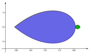
Figure 2. Left: An approximation to the real section of the immediate basin of attraction around a periodic point of order $4$ for $W_{Z^{3}+Z+t}$ with $t=177.68741192204597$. The coordinates shown are $(z_{1},z_{2})$; the corresponding point is $(z_{1},z_{2},-z_{1}-z_{2})$. The coloring encodes the number of iteration steps necessary to get within distance $10^{-4}$ of the periodic point. Right: Parameter values $t\in{\mathbb{C}}$ for which there exists a stable $4$-cycle of transposition type (left region, blue) or a stable $4$-cycle without extra symmetry (right region, green). The components touch at a point where the multiplier matrix under $\widetilde{W}_{p}^{\circ 2}$ has eigenvalue $-1$.

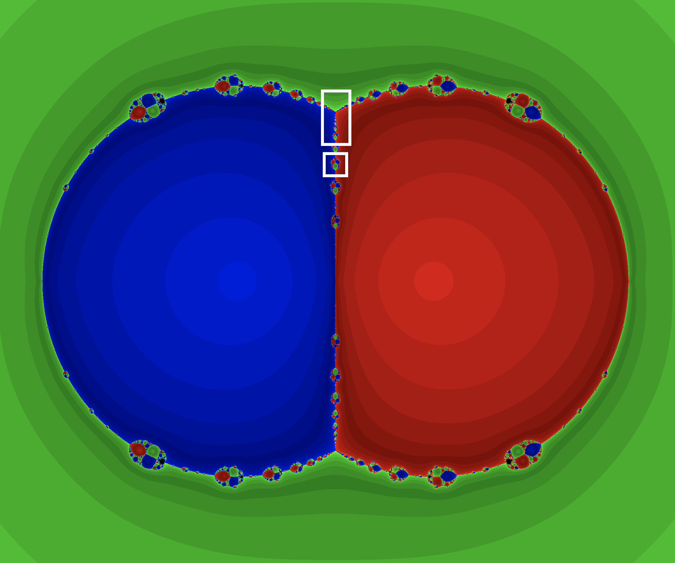
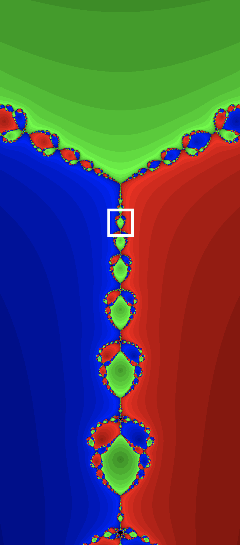
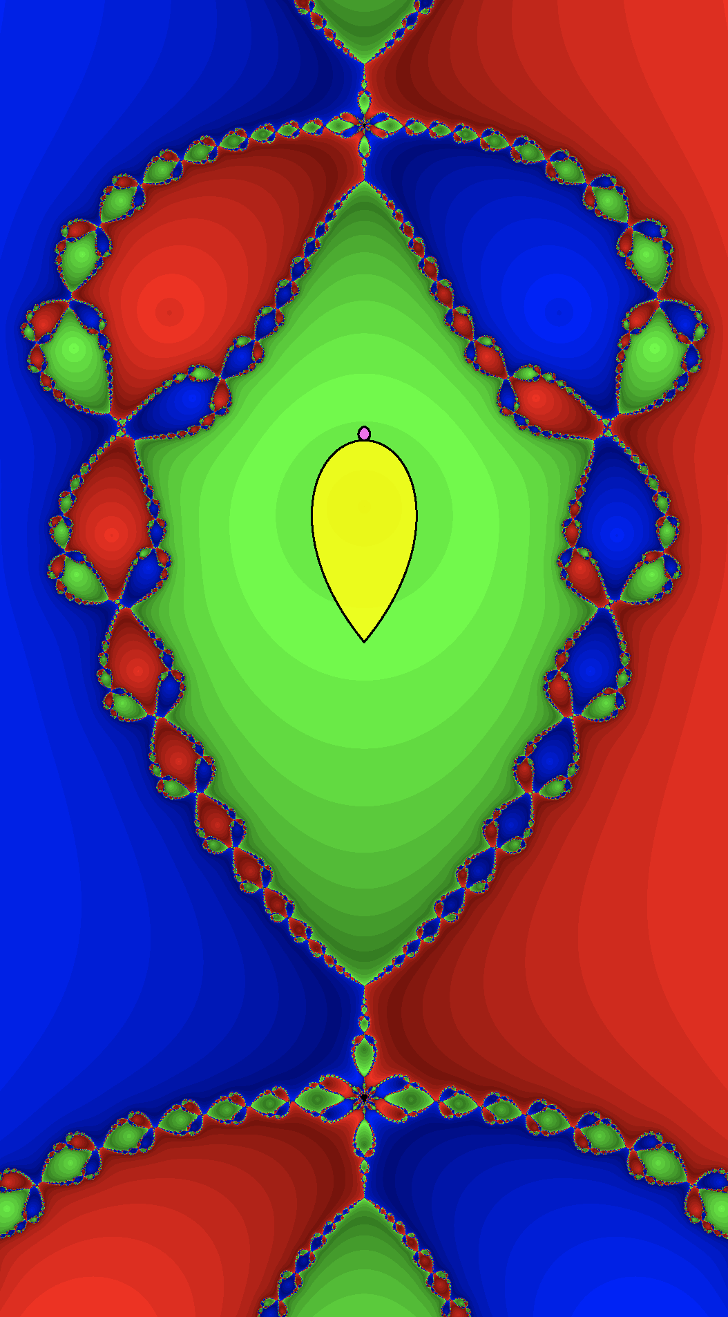
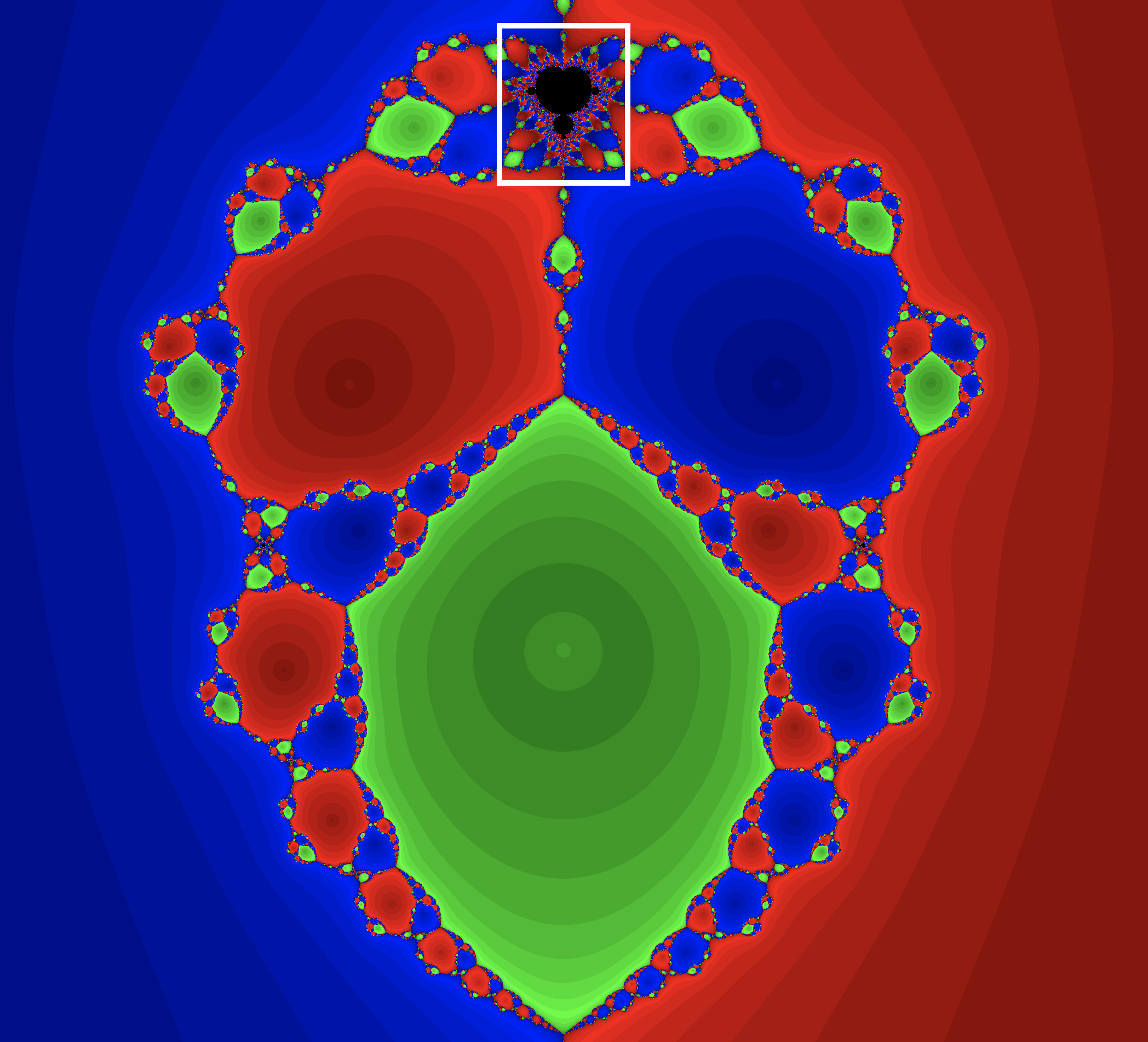
Figure 3. The parameter space of cubic polynomials up to affine precomposition, parameterized as $p(Z)=Z(Z-1)(Z-\lambda)$ with $\lambda\in{\mathbb{C}}$; shown is the complex $\lambda$-plane. This is the standard parameterization used in previous research on the Newton dynamics. The picture illustrates the Newton dynamics: the three colors indicate to which of the three roots $0$, $1$, and $\lambda$ the free critical point converges.
The picture on the left shows a global view of parameter space, with two subsequent magnifications shown in the middle and on the right. The regions shown on the right in Figure 2, which indicate parameter values for which an attractive $4$-cycle exists for the Weierstrass iteration, are superimposed on the last magnification (shown in yellow and magenta and converted to the different parameterization used here).

Figure 4. Sequence of refinements, starting with the first picture in Figure 4, towards the largest of the “little Mandelbrot sets” around attracting cycles of period $4$ for the Newton iteration (there are apparently larger little Mandelbrot sets on the outer circles; these represent conformally conjugate dynamics and seem larger only because of different parametrizations).

5.4   Points of order $6$

Finally, we consider $6$-cycles of rotation type.

Proposition 5.8.

The $6$-cycles of rotation type form two irreducible smooth curves of geometric genus $5$, each of degree $24$ over the $t$-line, that are permuted by a transposition of the coordinates. The characteristic polynomial $X^{2}+c_{1}X+c_{0}$ of the multiplier matrix at any associated point (considered as a point of order $2$ under $\tilde{W}_{p}$) satisfies a relation that specifies a curve of geometric genus $0$ and degree $5$. This curve can be parameterized as $(c_{0}(u)/c_{2}(u),c_{1}(u)/c_{2}(u))$, where

$$c_{0}(u) =-36u^{5}-12u^{4}+60u^{3}+236u^{2}+260u-4\,,$$

$$c_{1}(u) =-4u^{5}-51u^{4}-90u^{3}+59u^{2}+42u+5\,,$$

$$c_{2}(u) =-9u^{4}-18u^{3}+u^{2}+10u-1\,.$$

In particular, no such $6$-cycle can be attracting.

Proof.

We set up the variety describing $6$-cycles of rotation type as a subscheme of $5$-dimensional affine space with coordinates $t,x_{0},y_{0},x_{1},y_{1}$, where $t$ is the parameter and the iteration satisfies

$$(x_{0},y_{0},-x_{0}-y_{0})\longmapsto(x_{1},y_{1},-x_{1}-y_{1})\longmapsto(y_{0},-x_{0}-y_{0},x_{0})\,,$$

and we remove components coming from $3$-cycles of rotation type. This results in a smooth irreducible curve of degree $24$ over the $t$-line that has genus $5$. We find the image curve in the $(c_{0},c_{1})$-plane. Since the degree and the coefficient size are moderate, we can directly check that the curve has geometric genus $0$ and then find a parameterization. We then use the explicit equation and Lemma 5.2 with $\ell$ the negative real axis and $N=12$ to verify that no characteristic polynomial lying on the curve can have both roots in the unit disk. ∎

5.5   Proof of Theorem A

The results obtained in this section provide a proof of part (2) of Theorem A. Proposition 5.6 gives a proof of part (1) for the case $d=3$. To obtain the conclusion for all $d\geq 3$, we invoke Lemma 3.7.