Direct Measurement of the Hi–Halo Mass Relation through Stacking

Abstract

We present accurate measurements of the total Hi mass in dark matter halos of different masses at $z\sim 0$, by stacking the Hi spectra of entire groups from the Arecibo Fast Legacy ALFA Survey. The halos are selected from the optical galaxy group catalog constructed from the Sloan Digital Sky Survey DR7 Main Galaxy sample, with reliable measurements of halo mass and halo membership. We find that the Hi-halo mass relation is not a simple monotonic function, as assumed in several theoretical models. In addition to the dependence of halo mass, the total Hi gas mass shows strong dependence on the halo richness, with larger Hi masses in groups with more members at fixed halo masses. Moreover, halos with at least three member galaxies in the group catalog have a sharp decrease of the Hi mass, potentially caused by the virial halo shock-heating and the AGN feedback. The dominant contribution of the Hi gas comes from the central galaxies for halos of $M_{\rm h}<10^{12.5}h^{-1}M_{\sun}$, while the satellite galaxies dominate over more massive halos. Our measurements are consistent with a three-phase formation scenario of the Hi-rich galaxies. The smooth cold gas accretion is driving the Hi mass growth in halos of $M_{\rm h}<10^{11.8}h^{-1}M_{\sun}$, with late-forming halos having more Hi accreted. The virial halo shock-heating and AGN feedback will take effect to reduce the Hi supply in halos of $10^{11.8}h^{-1}M_{\sun}<M_{\rm h}<10^{13}h^{-1}M_{\sun}$. The Hi mass in halos more massive than $10^{13}h^{-1}M_{\sun}$ generally grows by mergers, with the dependence on halo richness becoming much weaker.

1 Introduction

How galaxies obtain their gas, form stars and quench, is the very basic question in understanding galaxy formation and evolution. In the standard paradigm of galaxy formation (e.g., Rees & Ostriker, 1977; Silk, 1977; White & Rees, 1978), gas infalling into a dark matter halo suffers from virial shock-heating around the halo virial radius, which impedes the efficiency of gas cooling. Detailed studies in simulations suggest that the virial shocks are only important above a critical shock-heating halo mass $\sim 10^{12}M_{\sun}$ (e.g., Birnboim & Dekel, 2003; Kereš et al., 2005; Dekel & Birnboim, 2006). While the feedback from active galactic nuclei (AGN) is also thought to be important around the similar halo mass scale (e.g., Di Matteo et al., 2005), it is then crucial to constrain the strength of AGN feedback from the relation between the cold gas mass and its host dark matter halo mass.

However, it is still observationally challenging to directly probe this relation. The majority of the cold gas in the universe is comprised of the neutral hydrogen. While the amount of atomic neutral hydrogen (Hi) can be reliably measured at $z\sim 0$ through the 21 cm hyperfine emission line, the molecular neutral hydrogen ($\rm{H_{2}}$) is generally difficult to probe directly. In the past decade, there have been lots of efforts to map the Hi distribution in the universe, e.g., the Hi Parkes All-Sky Survey (HIPASS; Barnes et al., 2001; Meyer et al., 2004), the Arecibo Fast Legacy ALFA Survey (ALFALFA; Giovanelli et al., 2005), and the GALEX Arecibo SDSS Survey (GASS; Catinella et al., 2010). There are only a few surveys to measure the $\rm{H_{2}}$ content using the tracer of CO emission lines, e.g., the COLD GASS survey (Saintonge et al., 2011), the Bima survey of nearby galaxies (BIMA SONG Helfer et al., 2003), the HERA CO-Line Extragalactic Survey (HERACLES Leroy et al., 2009), and the JINGLE survey (Saintonge et al., 2018). As the size and uniformity of existing Hi samples far exceed those of $\rm{H_{2}}$, we focus on Hi content in this work.

Another difficulty of constraining the Hi-halo mass relation is the estimation of the dark matter halo mass. Guo et al. (2017) measured the spatial clustering of the Hi-selected galaxies in the ALFALFA 70% sample and constrained the average halo masses for different Hi mass samples. More importantly, they found that the distribution of Hi-selected galaxies is not only dependent on the dark matter halo mass, but also related to the formation history of the host dark matter halos. Galaxies that are richer in Hi tend to live in halos formed more recently, which is generally referred to as the halo assembly bias effect (Gao et al., 2005). It complicates the Hi-halo mass relation with the additional dependence on other halo parameters related to the formation history. One such parameter is the halo angular momentum. There is various evidence that the Hi-rich galaxies tend to have higher halo spin parameters (e.g., Huang et al., 2012; Maddox et al., 2015; Obreschkow et al., 2016; Lutz et al., 2018). Therefore, it is necessary to include the effect of halo formation history when considering the Hi-halo mass relation.

Since blind Hi surveys like ALFALFA have selection effects arising from the Hi flux limit, as well as the dependence on the Hi line profile width ($W_{50}$) (Haynes et al., 2011), optically visible galaxies with low Hi fluxes and broad line profiles will not be detected in such radio surveys. Estimating halo masses for the ALFALFA-detected Hi sources essentially measures the relation of $\langle M_{\rm h}|M_{\rm HI}\rangle$ as in Guo et al. (2017), i.e., the average halo mass at a given Hi mass. It is significantly different from the relation of $\langle M_{\rm HI}|M_{\rm h}\rangle$, which measures the total Hi mass contained in halos of different masses, including those not detected by the observations (see e.g., Fig. 3 of Kim et al., 2017). While $\langle M_{\rm h}|M_{\rm HI}\rangle$ can only be used to quantify the halo mass for the Hi-rich galaxies detected by radio surveys, $\langle M_{\rm HI}|M_{\rm h}\rangle$ can be directly compared to the theoretical models with various quenching mechanisms that affect the total cold gas mass in different halos (see e.g., the review of Man & Belli, 2018). The measurement of $\langle M_{\rm HI}|M_{\rm h}\rangle$ is also important for current and future 21 cm intensity mapping projects, since the 21 cm power spectrum in the linear order is proportional to the product of the total Hi bias $b_{\rm HI}$ and the cosmic Hi abundance $\Omega_{\rm HI}$ (e.g., Villaescusa-Navarro et al., 2018; Obuljen et al., 2019; Wolz et al., 2019).

Although $\langle M_{\rm HI}|M_{\rm h}\rangle$ has been investigated extensively in different theoretical models, e.g., empirical models (Barnes & Haehnelt, 2014; Paul et al., 2018; Obuljen et al., 2019), semi-analytical models (Kim et al., 2017; Zoldan et al., 2017; Baugh et al., 2019) and hydrodynamical simulations (Villaescusa-Navarro et al., 2018), there still lacks direct observational measurement of this Hi-halo mass relation. Ai & Zhu (2018) have attempted to quantify the total Hi mass for rich galaxy groups with at least eight members using the detected sources in the ALFALFA 70% sample. They derived the group Hi mass fraction by summing up the Hi masses for all detected Hi sources and correcting for the missing ones based on the scaling relation between the Hi mass and those of galaxy luminosity and color. Given the large uncertainties in the Hi scaling relation for targets below the observational detection limit, one straightforward solution to properly take into account all the Hi emitting sources is to stack the Hi signals for entire galaxy groups with reliable halo mass estimates.

The Hi spectral stacking technique has previously been extensively applied in quantifying the relationships of Hi gas fraction with galaxy properties, such as stellar mass, color, star formation rate and stellar surface density (see e.g., Verheijen et al., 2007; Fabello et al., 2011; Geréb et al., 2015; Brown et al., 2015, 2017), as well as in constraining $\Omega_{\rm HI}$ at various redshifts (Lah et al., 2007; Delhaize et al., 2013; Rhee et al., 2013; Hu et al., 2019). Unlike with the traditional method of stacking the Hi spectra of single galaxies, applying Hi stacking to dark matter halos offers the great advantage that the stacking results should not be significantly affected by the spatial resolution of the Hi data, because the sizes of the dark matter halos are typically much larger than or at least comparable to the beam sizes of the radio telescopes. Therefore the effect of confusion from different halos would be minimal for such an experiment.

In this paper, we will directly measure $\langle M_{\rm HI}|M_{\rm h}\rangle$ by stacking the Hi spectra for dark matter halos selected from the galaxy group catalog. Such a stacking method is based on the single Hi spectrum from each entire group, which includes the contribution from all the Hi gas in the halos. The structure of the paper is as follows. In §2, we describe the galaxy samples. We briefly introduce our Hi stacking method in §3 and present the results in §4. We summarize and discuss the results in §5 and §6.

Throughout this paper, we assume a spatially flat $\Lambda$CDM cosmology, with $\Omega_{\rm m}=0.307$, $h=0.678$, $\Omega_{\rm b}=0.048$ and $\sigma_{8}=0.823$, consistent with the constraints from Planck (Planck Collaboration et al., 2014).

2 Data

2.1 The ALFALFA survey

The ALFALFA survey (Giovanelli et al., 2005) blindly mapped the Hi line emission over approximately 6900 deg² of the Northern sky in the redshift range $-2000<cz_{\odot}/\rm{km\,s^{-1}}<18000$. The survey utilized a two pass, drift scan strategy, with each second passage offset by half a beam width. This was extremely time efficient and resulted in highly uniform coverage. The survey footprint was split into two regions in the Northern Spring ($07^{\rm{h}}30^{\rm{m}}<\rm{RA}<16^{\rm{h}}30^{\rm{m}}$) and Fall ($22^{\rm{h}}<\rm{RA}<03^{\rm{h}}$) skies in the Declination range $0^{\circ}<\rm{Dec}<36^{\circ}$. The final source catalog (Haynes et al., 2018) contains over 30000 extragalactic sources.

In this work we focus exclusively on the Spring sky portion of the survey, as this is where there is appreciable overlap with the footprint of the Sloan Digital Sky Survey (SDSS) legacy spectroscopic survey (York et al., 2000). In the data processing stage, the survey area of ALFALFA is split into a pre-defined set of grids, with each grid square being 2.4^∘ on a side and spaced approximately 2^∘ apart. Each spatial grid is also divided into four overlapping ranges in heliocentric velocity, to make four spectral cubes for each spatial grid square (for further details refer to Haynes et al., 2011, 2018). Each spectral cube has dimensions of $144\times 144\times 1024$ corresponding to a pixel angular size of 1′, or approximately a quarter of the beam diameter ($3.8\arcmin\times 3.3\arcmin$). In addition to maps of the Hi line flux density, each cube contains a normalized weight map which indicates how much of the input data have been flagged for poor quality or radio frequency interference (RFI) at any given point in the cube. The typical rms noise of the data is approximately 2 mJy per 5 $\mathrm{km\,s^{-1}}$ channel, although the data are Hanning smoothed to a spectral resolution of about 10 $\mathrm{km\,s^{-1}}$.

2.2 Galaxy Group catalog

In order to stack the Hi signals for galaxy groups in the SDSS region, we use the SDSS galaxy group catalog from Lim et al. (2017), which is an extension to the early SDSS group catalog of Yang et al. (2007). This group catalog is based on the SDSS DR7 Main Galaxy Sample (Albareti et al., 2017), but it incorporates the redshifts for the missing galaxies due to fiber collisions from different sources (e.g. the later Data Release 13 and other surveys). We refer the readers to Lim et al. (2017) for more details. We adopt their SDSS group catalog with all galaxies having spectroscopic redshifts, which is about 98% complete compared to the full target sample. The halo masses in this group catalog are estimated using the proxy of galaxy stellar mass. The halo radius $r_{200}$ is estimated from the definition that the mean mass density within $r_{200}$ is 200 times the mean density of the universe at the given redshift, i.e.,

$$M_{\rm h}=200\bar{\rho}_{\rm m}(1+z)^{3}\frac{4\pi}{3}r_{200}^{3}$$ (1)

where $\bar{\rho}_{\rm m}$ is the mean background density of the universe at $z=0$.

The halo mass estimates in Lim et al. (2017) have been demonstrated to be unbiased using mock catalogs. The typical scatter is less than $0.2$ dex. As shown in their Figures 7 and 8, halos with $\log(M_{\rm h}/M_{\sun})>11.5$ are all complete at $z<0.05$ within the SDSS. As will be discussed in Section 4.2.1, although the SDSS DR7 galaxy catalog is a flux-limited sample, galaxies in the observed halos are basically complete above the stellar mass of $M_{\ast}>10^{9.5}h^{-2}M_{\sun}$, which means that the galaxy group catalog is missing some low-mass galaxies. This has two direct implications. Firstly, it emphasizes the importance of stacking the total Hi signal for each halo, rather than stacking the Hi spectra for the observed halo member galaxies, which will be biased towards the gas-rich massive galaxies. As the SDSS target sample selection is based on the galaxy luminosity, we do not expect any strong selection bias when we stack halos in different mass bins. So even though halos are not complete for $\log(M_{\rm h}/M_{\sun})<11.5$, the stacking measurements do not suffer from the selection effects. Secondly, the richness information for each halo in the group catalog, i.e., the number of member galaxies, is associated with certain stellar mass thresholds. We find that the halo richness is reliable for galaxies with $M_{\ast}>10^{7}h^{-2}M_{\sun}$.

For the purpose of matching the ALFALFA survey depth, we limit the redshift range of the halos in the group catalog to be $0.0025<z<0.06$, and we only use the group galaxies in the ALFALFA Spring sky. The final sample includes $28,910$ groups and $53,653$ galaxies . By cross-matching with the ALFALFA final source catalog, we find that only $15,211$ galaxies have measured Hi masses, i.e. the majority of the galaxies in the group catalog are below the ALFALFA detection limit (Haynes et al., 2011). It further emphasizes the importance of using the Hi signal stacking method to measure reliably the average Hi mass in each halo mass bin (Jones et al., 2020).

3 Stacking Method

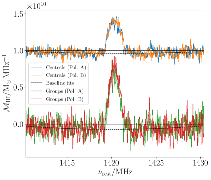
Figure 1: Example stacked spectra for both centrals and groups before the re-baselining was performed. These data are for the $12.25<\log(M_{\mathrm{halo}}/h^{-1}\,\mathrm{M_{\odot}})<12.5$ bin and for groups with at least 3 members. The centrals-only stack is vertically offset to show both spectra in the same figure. The two linear polarizations are shown for each spectrum with different colors and the 2nd order polynomial baseline fits are shown with dashed black lines.

In this work we use the ALFALFA IDL stacking software developed by Fabello et al. (2011) to extract spectra of each group and central in the group catalog. This software spatially integrates over a square aperture and returns a 1-dimensional spectrum of the Hi flux density. The velocity range covered corresponds to the entire range of the ALFALFA spectral cube with the nearest centre frequency to the expected frequency of the Hi emission of the target object, given its redshift. In addition to the flux density, a weight spectrum, integrated over the same sky aperture, is also generated, allowing us to track the impact of missing or poor quality data or contamination by RFI.

While Fabello et al. (2011) used a fixed aperture size for all stacked galaxies, the groups are frequently considerably larger than the single ALFA beam width. Therefore, each of our apertures is tailored to each group or central. We use the $r_{200}$ values to define the angular size of the aperture ($2r_{200}$) for each group, rounded up to a whole number of arcmin (pixels). The apertures for the centrals were all conservatively chosen to be 200 kpc in diameter. The latest measurement of the Hi size–mass relation shows that the largest Hi discs are between 100 and 200 kpc in diameter (see e.g., Figure 1 of Wang et al., 2016). Thus, this choice of aperture ensures that Hi flux from a target central galaxy will not be missed. The Hubble distance for each group was used to convert this to an angular size, which was again rounded up to an integer number of arcmin. This choice of aperture for the centrals undoubtedly leads to considerable contributions from confused emission, which we discuss further in the following sections. In both cases, we set a minimum aperture diameter of 8′ (approximately two beam widths). This means that for groups with distances greater than $\sim$85 Mpc, the aperture for the central will be larger than 200 kpc, likely leading to additional confusion.

In order to avoid re-gridding the ALFALFA data, any groups (and their centrals) which overlapped a boundary of the cube that contained them (specifically the one with the nearest center position on the sky) were discarded. This resulted in the removal of approximately 2% of the groups (centrals). The four spectral cubes that each ALFALFA grid square is divided into overlap with the neighboring cube by $\sim$700 $\mathrm{km\,s^{-1}}$, while the velocity dispersion estimated by Lim et al. (2017) for a group of $\log(M_{\rm{halo}}h^{-1}/M_{\odot})=14$ is 418 $\mathrm{km\,s^{-1}}$. Therefore, the velocity axis was ignored when making these cuts.

The spectrum extraction process was performed for every group and central available. Of the total groups and centrals in the catalog, 25906 group spectra (90%) and 25868 (89%) central spectra were successfully extracted from the ALFALFA cubes. The targets which were not extracted were discarded due to the low weight of their spectra or proximity to grid boundary as described in the previous paragraph. The spectral extraction software of Fabello et al. (2011) discards spectra if more than 40% of the channels have a weight value of less than 0.5. In practice these spectra would mainly contribute noise to any stacks because too much of their data has been flagged for RFI or is missing coverage. The successfully extracted spectra were then divided into halo mass bins and separate stacks produced for each mass bin. This will be described further in the next section. The following paragraphs describe how the extracted spectra were stacked in a general sense.

Once the spectra were extracted, we combined them using our own Python script. Each spectrum is shifted such that the expected frequency of its Hi emission falls in the central channel of the stack spectrum. This is done to the nearest channel ($\sim$5 $\mathrm{km\,s^{-1}}$) so that the spectra do not need to be re-binned. The individual spectra are then converted from units of mJy to $\rm{M_{\odot}\,MHz^{-1}}$ following equation 45 of Meyer et al. (2017). Any regions of the spectra which have a normalized weight value of less than 50% are discarded, as these regions can contain residual unflagged bright RFI. We also discard any spectra with spikes that exceed 100 times the expected rms noise, as these would contribute a lot of noise to the final stack. In total, this results in 24443 groups which contribute to the final stacks. The spectra are co-added with each weighted by $1/\sigma_{\rm{rms}}^{2}$. Here the rms noise in mJy (not $\rm{M_{\odot}\,MHz^{-1}}$) is used to avoid the weighting being distance dependent. Throughout this process the two polarizations recorded in ALFALFA were treated entirely independently, which provided an additional means to verify that there was no polarized interference affecting the final stacks.

To measure the Hi mass in each stack, the stack spectra need to first be re-baselined. We observed that the continuum level in the stacks was generally slightly negative, probably because the original ALFALFA baselining procedure fit within regions containing line emission, but at extremely low SNR (i.e. SNR $<$ 1), such that it can only be perceived in stacks of hundreds of targets. The central 20 MHz of the stack spectrum (with the inner central 5 MHz excluded) was used to fit and remove a 2nd order baseline (Figure 1).

From this point onward, stacks of centrals and stacks of groups were treated differently. The peak of stacked Hi emission in a group stack was fit with a Gaussian profile and the flux (measured, not the fit) within $\pm 3\sigma$ was summed to estimate the average Hi mass of the groups in the stack. For the stacks of centrals we did not fit a Gaussian to the profiles because, in most cases, considerable confusion was likely. Instead we summed all emission within a $\pm$300 $\mathrm{km\,s^{-1}}$ window. Very few galaxies have Hi line widths greater than 600 $\mathrm{km\,s^{-1}}$ (e.g Papastergis et al., 2011), meaning this window will contain all the targeted line emission, except in extreme cases.

The final step of the stacking process was to estimate the uncertainties in the stack masses. This was done through bootstrapping the entire stacking process. For each final stack, 1000 iterations were generated where the input catalogue of targets was randomly sampled (with replacement) to construct a bootstrap sample of the same size. The uncertainty in the mass measurements was taken as the standard deviation of these 1000 iterations.

4 Results

4.1 Hi-Halo Mass Relation

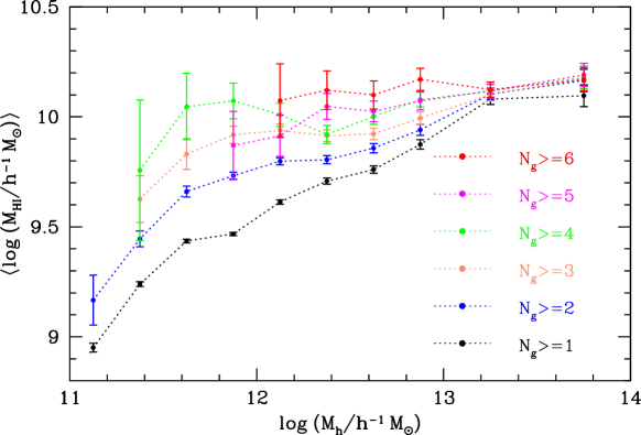
Figure 2: Measurements of total Hi masses for halos in different mass bins. We show the measurements for different richness groups in different colors as labeled. There is an increasing turn-over feature with larger group richness around the halo mass scale $\sim 10^{12}M_{\sun}$.

We show in Figure 2 the average Hi-halo mass relation, i.e., $\langle M_{\rm HI}|M_{\rm h}\rangle$, from our Hi spectral stacking technique. The points with the black dotted line are the measurements using all the halos for which we extracted spectra. We also present the measurements for halos of different richness $N_{\rm g}$, i.e. number of member galaxies in the group catalog, shown as points and dotted lines with different colors. We find that there is a clear dependence of the Hi-halo mass relation on the halo richness. Halos with higher richness (at fixed halo mass) generally tend to have larger average Hi masses.

We note that the total Hi mass in the halo is not a simple monotonically increasing function of the halo mass. The total Hi mass in halos of $N_{\rm g}\geq 2$ tends to increase to a plateau around $M_{\rm h}\sim 10^{12.4}h^{-1}M_{\sun}$ and then sharply increase again. For halos with richness $N_{\rm g}\geq 3$ and $N_{\rm g}\geq 4$, there is a pronounced bump feature in the Hi-halo mass relation for $M_{\rm h}<10^{12.5}h^{-1}M_{\sun}$ with the peak at around $M_{\rm h}\sim 10^{11.9}h^{-1}M_{\sun}$. For halos of higher richness of $N_{\rm g}\geq 5$, we are not able to clearly detect such a feature, due to the large errors in the measurements and lack of low-mass halos with a high richness.

For halos with richness of $N_{\rm g}\geq 6$, $\langle\log(M_{\rm HI}/h^{-1}M_{\sun})\rangle$ approaches a constant of $10.1$, without any strong dependence on the halo mass. We have stacked halos of higher richness and find the same behavior. It provides a direct estimate of the total Hi mass for rich galaxy clusters with different halo masses. At the massive end, more and more halos have multiple member galaxies and the dependence on the halo richness seems to become much weaker.

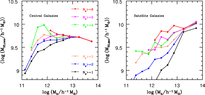
Figure 3: Similar to Figure 2, but for the contributions from the central galaxies (left panel) and from the summation of all satellite galaxies (right panel) in each halo. For clarity, the error bars of the measurements are omitted.

Figure 4: Left: comparison between the halo mass function $n(M_{\rm h})$ from the group catalog (dotted line) and that of the same cosmology directly obtained from the TNG100 simulation (solid line) of the IllustrisTNG simulation set. Right: observed galaxy stellar mass function in the group catalog (crosses), in comparison to the intrinsic measurement of Li & White (2009) (solid line). The stellar mass function corrected for the halo completeness is displayed as the dotted line.

In order to separate the contribution to the total Hi mass into different components, we show in Figure 3 the average Hi mass from the central galaxies (left panel) and from the summation of all satellite galaxies (right panel) in halos of different masses, respectively. Measurements for halos of different richness thresholds are shown as different color lines. For clarity, the error bars of the measurements are omitted. As we have stacked the Hi spectra for the central galaxies, the contribution of all satellite galaxies in each halo mass bin to the total Hi mass is simply obtained by subtracting the Hi mass in the central galaxies from those of the halos. However, as we noted before, stacking the Hi signals of the central galaxies would be contaminated by the confusion from the nearby satellite galaxies. Therefore, the measurements of the Hi mass in the centrals are upper limits, while those of the satellites are lower limits. We will discuss the effect of confusion in Section 4.2.2.

The central galaxies dominate the contribution to the total Hi mass for low-mass halos, while the contribution from the satellite galaxies become comparable and even larger for halos of $M_{\rm h}>10^{12.5}h^{-1}M_{\sun}$. We note that the bump feature in the Hi-halo mass relation is caused by the contribution from central galaxies, while the contribution from satellites monotonically increases with halo mass. At low halo masses, centrals with more surrounding satellites have higher Hi masses, but above $M_{\rm h}=10^{13}h^{-1}M_{\sun}$ this trends disappears. Moreover, the effect of halo richness on $\langle\log M_{\rm HI}\rangle$ becomes increasingly smaller for larger $N_{\rm g}$.

The $\langle\log M_{\rm HI}\rangle$ for all satellite galaxies seems to follow power-law relations, with smaller slopes for higher halo richnesses. The trend with the halo richness is also similar to that of the central galaxies, but without the bump feature. In massive halos of $M_{\rm h}>10^{13}h^{-1}M_{\sun}$, the majority of the Hi mass is contributed by the satellite galaxies. The values of $\langle M_{\rm HI}|M_{\rm h}\rangle$ for all halos (i.e., $N_{\rm g}\geq 1$), as well as the corresponding values for the central galaxies, are displayed in Appendix A.

4.2 Systematic Effects

Before discussing the implications of our measurements, we will first verify the results with several systematic tests.

4.2.1 Sample Completeness

The first question is whether the trend of Hi-halo mass relation with the halo richness could be significantly affected by the incompleteness of the galaxy sample. Since the SDSS DR7 Main Galaxy Sample is flux-limited, we will miss faint galaxies at high redshifts. As we focus on the redshift range of $0.0025<z<0.06$ with available ALFALFA data, the sample is volume-limited for galaxies with a $r$-band absolute magnitude brighter than $M_{\rm r}\sim-18.8$ (see e.g., Fig. 1 of Guo et al., 2015), which corresponds to a galaxy stellar mass threshold around $10^{9.5}h^{-2}M_{\sun}$. Therefore, some of the gas-rich but optically faint galaxies in this redshift range might be missed in the group catalog due to the optical flux limit, which will affect the richness estimates of the halos. But the contribution of their Hi flux to the host halo are correctly included through the stacking method.

The galaxy sample completeness as a function of stellar mass, $C_{\rm g}(M_{\ast})$, can be separated into the completeness of halos with a given mass $M_{\rm h}$, $C_{\rm h}(M_{\rm h})$, and the completeness of galaxies with a stellar mass $M_{\ast}$ in these halos, $C_{\rm g}(M_{\ast}|M_{\rm h})$. We are then dividing the missing galaxies into those in the missing halos and those in the observed halos. As there is no obvious selection bias of the halo population at a given mass for the flux-limited SDSS sample, the detected halos would be representative of the whole population. Then the halo richness estimate is only affected by $C_{\rm g}(M_{\ast}|M_{\rm h})$. The advantage of the group catalog is that we can estimate $C_{\rm g}(M_{\ast})$ and $C_{\rm h}(M_{\rm h})$ directly from comparing to the intrinsic values from simulations and observations.

We show in the left panel of Figure 4 the comparison between the halo mass function $n(M_{\rm h})$ from the group catalog (dotted line) and that of the same cosmology directly obtained from the TNG100 simulation (solid line) of the IllustrisTNG simulation set (Marinacci et al., 2018; Naiman et al., 2018; Nelson et al., 2018; Pillepich et al., 2018; Springel et al., 2018). The dark matter halos in the group catalog is basically complete for $M_{\rm h}>10^{11.5}h^{-1}M_{\sun}$, while the completeness decreases to around $1\%$ for halos of $M_{\rm h}\sim 10^{11}h^{-1}M_{\sun}$. The right panel of Figure 4 shows the observed galaxy stellar mass function (SMF) in the group catalog (crosses), in comparison to the intrinsic measurement of Li & White (2009) (solid line) obtained by up-weighting galaxies with the maximum detectable volumes in $0.0025<z<0.06$. The observed galaxies are complete for $M_{\ast}>10^{10}h^{-2}M_{\sun}$, and the completeness $C_{\rm g}(M_{\ast})$ decreases to 6% for $M_{\ast}\sim 10^{8}h^{-2}M_{\sun}$.

As we have estimated the halo completeness, we can correct the effect of missing halos through weighting each galaxy by the corresponding value of $1/C_{\rm h}(M_{\rm h})$. The resulting SMF is shown as the dotted line. With the correction, we find that the galaxies in the observed halos are complete for $M_{\ast}>10^{9.5}h^{-2}M_{\sun}$. The stellar mass completeness is 60% for $M_{\ast}\sim 10^{9}h^{-2}M_{\sun}$ and decreases to 25% for $M_{\ast}\sim 10^{8}h^{-2}M_{\sun}$. Therefore, we are still missing some low-mass galaxies for the observed halos. As the low-mass halos are not likely to host many satellite galaxies, the majority of the missing galaxies would possibly be dwarf satellite galaxies in massive halos.

The value of a halo richness is then only meaningful with a stellar mass threshold, as we will always be missing those very low-mass galaxies. If we set the galaxy stellar mass threshold to be $M_{\ast}>10^{7}h^{-2}M_{\sun}$, more than $99.5\%$ of the observed halos would have the same richness values as provided in the group catalog. Thus, for fair comparisons with the theoretical models in the following sections, the halo richness $N_{\rm g}$ is defined as the number of galaxies with $M_{\ast}>10^{7}h^{-2}M_{\sun}$ in each halo.

4.2.2 Confusion Correction

As the Hi spectral stacking technique simply cuts out a square box centered on the target position, it is inevitable that this includes some amount of confused Hi emissions from nearby objects in both the angular and radial directions. In order to estimate the effect of confusion, we can apply corrections to the Hi mass measurements for halos and central galaxies separately.

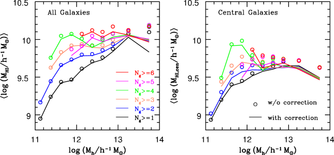
Figure 5: Effect of applying the confusion correction to the Hi-halo mass relations for the halos (left panel) and central galaxies (right panel). The open circles are the original measurements, while the solid lines are those with confusion corrections (see text for details).

As noted in Section §3, the angular aperture size of the stacking for each halo is $\max(2r_{200}/D_{\rm A},8\arcmin)$, where $r_{200}$ and $D_{\rm A}$ are the virial radius and the angular diameter distance of the halo, respectively. In the radial direction, we integrate the Hi flux within $3\sigma$ of the peak of the stacked spectra for each halo mass bin. As shown in the stacked spectra in Appendix B, the $3\sigma$ velocity range of the low-mass halos of $M_{\rm h}\sim 10^{11}h^{-1}M_{\sun}$ is only around 150 $\mathrm{km\,s^{-1}}$, but increases to around 1000 $\mathrm{km\,s^{-1}}$for halos of $M_{\rm h}\sim 10^{14}h^{-1}M_{\sun}$.

In order to estimate the contribution from confused Hi emission for the group halos, we employ a correction as follows. For each halo mass bin, we identify all the non-target halos from the group catalog which are within the apertures (angular and radial) used to stack the targets. Using the uncorrected relations from Figure 2, we can derive the average Hi mass in given halo mass and richness bins, $\langle M_{\rm HI}|M_{\rm h},N_{\rm g}\rangle$, by subtracting the measurements between the two neighbouring richness threshold samples. We then estimate the Hi masses of these companion halos and thus how much they contribute to the stacked spectra in the relevant halo mass bin.

As halos in the group catalog are quite complete for $M_{\rm h}>10^{11.3}h^{-1}M_{\sun}$, we can get a reliable estimate of the number of companion halos in each mass bin. We find that for $M_{\rm h}<10^{12.5}h^{-1}M_{\sun}$, the average number of companion halos for each halo is typically smaller than $0.05$. It slightly increases to $0.3$ for $M_{\rm h}\sim 10^{13}h^{-1}M_{\sun}$ and becomes around $1.5$ for for $M_{\rm h}\sim 10^{14}h^{-1}M_{\sun}$. The correction to the Hi-halo mass relation is shown in the left panel of Figure 5 for halos with different richnesses, with the circles for the original measurements and lines for the corrected ones.

We note that our correction is an over-estimate of the real effect, as we simply assume the overlapping fraction between the confused halo and companions to be unity, different from the implementation of Fabello et al. (2011). Despite this, we find that the correction is basically minor for halos of $M_{\rm h}<10^{13}h^{-1}M_{\sun}$, but becomes very significant for the largest halo mass bin of $10^{13.5}<M_{\rm h}<10^{14}h^{-1}M_{\sun}$. As shown in Figure 9, due to the small number of available halos, the large noises in the stacked spectra of the most massive halos make the confusion correction less reliable.

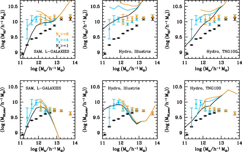
Figure 6: Comparisons between the Hi-halo mass relation measurements of observation (points) and different theoretical models (lines). The top and bottom panels are for the measurements of halo and central galaxies, respectively. The left, middle, and right panels are for the L-GALAXIES semi-analytical model, the Illustris, and IllustrisTNG hydrodynamical simulation models, respectively. For illustration, we only show three typical cases with the halo richnesses of $N_{\rm g}\geq 1$ (black), $N_{\rm g}\geq 4$ (blue), and $N_{\rm g}\geq 6$ (orange).

The confusion correction for the stacking of central galaxies is treated differently. The angular aperture size for central galaxies is $\max(200\,\rm{kpc}/D_{\rm A},8\arcmin)$, and we summed all emission within 300 $\mathrm{km\,s^{-1}}$of the peak values. Due to the large aperture size, the centrals are very likely to be confused with nearby satellite galaxies. The confusion effect would then become much larger for more massive halos with multiple satellites and this is compounded by the fact that satellites dominate the Hi content of massive halos. The average number of companion galaxies for each central is around $0.2$ for $M_{\rm h}\sim 10^{12}h^{-1}M_{\sun}$ and increases to $0.8$ for $M_{\rm h}\sim 10^{13}h^{-1}M_{\sun}$. So the confusion effect is much larger for central galaxies, compared to that of the halo. Moreover, the confusion effect of central galaxies would significantly increase with the halo richness, as expected.

The confusion correction for the central galaxies is, however, hard to estimate. Because only less than 30% of the individual galaxies in the group catalog have available Hi masses in the ALFALFA survey. As a lower limit of the confusion effect, we apply a minimal correction to the total Hi masses of the central galaxies by only subtracting the companions with measured Hi masses. The result is shown in the right panel of Figure 5. The correction is in general around 0.1 dex for halos of $M_{\rm h}>10^{12}h^{-1}M_{\sun}$, but becomes much smaller for low-mass halos with a small richness. But the overall trend of $\langle M_{\rm HI}\rangle$ with the halo mass and richness is still quite similar to ones without correction.

We can also estimate the Hi masses for those galaxies without ALFALFA detection by applying the scaling relations of the gas fraction with the optical galaxy properties (Fabello et al., 2012), e.g., color and surface brightness, as in Zhang et al. (2009) and Li et al. (2012). While such Hi mass estimators have large scatters of around 0.3 dex, we find that the confusion correction would reach to about 0.2 dex for halos of $M_{\rm h}\sim 10^{12}h^{-1}M_{\sun}$ and 0.3 dex for the most massive halos. It is thus essential to have reliable Hi mass estimates for the companions. Therefore, the stacking of the central galaxies can be deemed as upper limits of the total Hi mass content.

We note that the halo mass estimate and central/satellite assignment in the group catalog are never perfect (Campbell et al., 2015). There are inevitable measurement errors for the halo mass estimates. However, the typical halo mass error is around 0.2 dex, which corresponds to a small error of 0.067 dex for the halo virial radius, as $r_{200}\propto M_{\rm h}^{1/3}$. Moreover, the errors in the halo mass estimates are relatively compensated by our stacking of the halos. While our measurements of the Hi-halo mass relation would potentially be slightly smoothed by the halo mass errors, the overall trend with the halo richness would not be affected. The mis-assignment of central and satellite galaxies is not a significant effect in our measurements, as we do not focus on the individual central and satellite galaxies.

4.3 Comparison to theoretical models

While our direct measurements of the Hi-halo mass relations show a strong dependence on the halo richness, it is important to compare with the theoretical model predictions. We show in Figure 6 the comparisons of $\langle M_{\rm HI}|M_{\rm h}\rangle$ for halos (top panels) and central galaxies (bottom panels) of different theoretical models. Our measurements are displayed as the symbols with error bars, while the model predictions are represented by the solid lines. We consider the L-GALAXIES semi-analytical model of Fu et al. (2013) (left panels), the hydrodynamical simulations of Illustris (Vogelsberger et al., 2014) (middle panels) and IllustrisTNG (right panel). For illustration, we only show three typical cases with the halo richnesses of $N_{\rm g}\geq 1$, $N_{\rm g}\geq 4$, and $N_{\rm g}\geq 6$, as symbols and lines of different colors.

The division of neutral hydrogen into Hi and H₂ in the Illustris and IllustrisTNG simulation models is implemented following Diemer et al. (2018), based on the Hi/H₂ transition model of Krumholz (2013). It has been shown that while the Illustris model significantly over-predicts the abundance of Hi gas (Guo et al., 2017), the IllustrisTNG model agrees much better with the observation (Diemer et al., 2019; Stevens et al., 2019). The Hi/H₂ transition in the L-GALAXIES model adopts the prescription of Blitz & Rosolowsky (2006), which is based on the pressure in the local ISM.

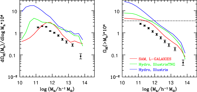
Figure 7: Fractional contribution to $\Omega_{\rm HI}$ of different halo mass bins $d\Omega_{\rm HI}/d\log M_{\rm h}$ (left panel), and the cumulative contribution of $\Omega_{\rm HI}(>M_{\rm h})$ above a given halo mass threshold (right panel). Our measurements are displayed as the points, while solid lines of different colors represent the three theoretical models. The dotted line in the right panel is the measurement from the Hi mass function of ALFALFA 100% sample (Jones et al., 2018).

Our stacking is based on the optical galaxies in the group catalog, but the different theoretical models have quite different galaxy stellar mass function predictions, which are not always consistent with the observation. Therefore, fair comparisons between observations and models should be made for galaxy samples above different stellar mass thresholds, but with the same number density. As stated before, our halo richness definition is consistent with a stellar mass threshold of $M_{\ast}>10^{7}h^{-2}M_{\sun}$. We calculate the “complete” sample number density by summing all galaxies with $M_{\ast}>10^{7}h^{-2}M_{\sun}$ from the SMF measurement of Li & White (2009), as in the right panel of Figure 4. The resulting sample number density is $0.0696\,h^{-3}\,\rm{Mpc}^{3}$. The corresponding stellar mass thresholds for the L-GALAXIES, Illustris, and IllustrisTNG models are $10^{8.62}h^{-2}M_{\sun}$, $10^{8.75}h^{-2}M_{\sun}$, and $10^{8.30}h^{-2}M_{\sun}$, respectively. The stellar mass thresholds in different models are comparable, but much higher than the observation.

As shown in Figure 6, the same dependence on the halo richness is found in all the models, which confirms our finding. However, none of the models can well reproduce the observed Hi-halo mass relations. From the top panels of Figure 6, all three models significantly over-predict the total Hi mass for halos of $M_{\rm h}>10^{11.5}h^{-1}M_{\sun}$ and $N_{\rm g}\geq 1$. As we will show in the following, the excess of the Hi gas will result in the over-prediction of cosmic Hi gas density, $\Omega_{\rm HI}$.

As noted before, the central and satellite galaxies dominate over the contribution to the total Hi gas for halos below and above the transition mass $M_{\rm h}\sim 10^{12.5}h^{-1}M_{\sun}$, respectively. By comparing the top and bottom panels of Figure 6, we find that the L-GALAXIES model tends to agree with our measurements at the low halo mass end for both $N_{\rm g}\geq 1$ and $N_{\rm g}\geq 4$. However, the amount of Hi gas in the satellite galaxies in the massive halos is over-predicted. The situation is quite similar for the Illustris model, but the satellite contribution of the cold Hi gas in low-mass halos is too high. However, the improved IllustrisTNG hydrodynamical simulation model tends to put too little cool gas in the satellite galaxies in massive halos. The central galaxies contribute the majority of the Hi gas in halos of all masses.

It is noteworthy that the bump feature of the Hi-halo mass relation is observed in all three models, but with different strengths. As explained in Baugh et al. (2019), the turn-over of $\langle M_{\rm HI}\rangle$ around halos of $M_{\rm h}\leavevmode\nobreak\ \sim 10^{12}h^{-1}M_{\sun}$ is generally assumed to be caused by the suppression of gas cooling by Active Galactic Nuclei (AGN) feedback. It seems that the low level of AGN feedback in the IllustrisTNG models makes the gas cooling too efficient in the massive halos. Therefore, our measurements can potentially be used to constrain the strength of AGN feedback.

4.4 Cosmic Neutral Hydrogen Gas Density

With the Hi-halo mass relation, we can estimate the cosmic Hi gas density as,

$$\Omega_{\rm HI}=\frac{1}{\rho_{\rm c}}\int\langle M_{\rm HI}|M_{\rm h}\rangle n(M_{\rm h})dM_{\rm h},$$ (2)

where $n(M_{\rm h})$ is the intrinsic halo mass function and $\rho_{\rm c}$ is the critical density. The measurement of $\Omega_{\rm HI}$ can be directly compared with the one obtained from integrating the Hi mass function (see e.g., Martin et al., 2010; Jones et al., 2018). However, as we only measure $\langle M_{\rm HI}|M_{\rm h}\rangle$ for halos more massive than $10^{11}h^{-1}M_{\sun}$, a proper extrapolation is necessary to obtain an accurate estimate of $\Omega_{\rm HI}$. The extrapolation for the Hi mass function is done using the Schechter function (Martin et al., 2010). We reserve the investigation of the proper functional form for the Hi-halo mass relation to our future work.

Using our current measurements, we can calculate the fractional contribution to $\Omega_{\rm HI}$ of different halo mass bins, $d\Omega_{\rm HI}/d\log M_{\rm h}$, and the cumulative contribution of $\Omega_{\rm HI}(>M_{\rm h})$ above a given halo mass threshold. We show (in Figure 7) our measurements as the points, while solid lines of different colors represent the three theoretical models. The dotted line is the measurement from the Hi mass function of ALFALFA 100% sample (Jones et al., 2018). The predicted $\Omega_{\rm HI}$ is $3.5\times 10^{-4}$ before applying the correction for Hi self-absorption, which is estimated to be 11% in Jones et al. (2018). However, the self-absorption correction for the stacking of halos is very difficult to estimate, so we ignore the self-absorption correction in our measurements.

We find that the cumulative Hi density $\Omega_{\rm HI}(M_{\rm h}>10^{11}h^{-1}M_{\sun})$ is $2.5\times 10^{-4}$. Thus, there is still about 30% of the total Hi gas in halos of $M_{\rm h}<10^{11}h^{-1}M_{\sun}$, where the dwarf central galaxies would dominate the Hi mass contribution. Observation of these faint galaxies in future surveys would provide better constraints on $\Omega_{\rm HI}$. We note that all three theoretical models over-predict the cumulative contribution to $\Omega_{\rm HI}$, due to the overestimate of the Hi mass in massive halos. For the fractional contribution of $d\Omega_{\rm HI}/d\log M_{\rm h}$, the L-GALAXIES model shows better agreement than the two simulation models. The majority of the Hi mass is contributed by halos of $M_{\rm h}<10^{12}h^{-1}M_{\sun}$, which is consistent with the predictions of Guo et al. (2017) that most of the Hi-rich galaxies live in halos of $M_{\rm h}<10^{12}h^{-1}M_{\sun}$.

5 Discussion

The dependence of the total Hi mass on the halo richness in addition to the dependence on the halo mass reflects the halo assembly bias effect of Hi-rich galaxies. The halo assembly bias is generally referred to as the additional dependence of halo bias on properties of the halo formation history (see e.g., Gao et al., 2005; Gao & White, 2007; Jing et al., 2007). As found in Guo et al. (2017), for halos of a given mass, those with a later formation time tend to host galaxies with a larger Hi mass. As shown in Figure 5 of Wechsler et al. (2006), halos with later formation times have higher richness values. Therefore, our finding of the richness dependence is fully consistent with the conclusion of Guo et al. (2017). They both confirm that the Hi mass is directly connected to the halo formation history.

The commonly used indicators to characterize the halo formation history include the halo formation time, the spin parameter and the concentration parameter. The behavior of the halo assembly bias effect with the halo mass is quite different for the different indicators. For massive halos of $M_{\rm h}>10^{13}h^{-1}M_{\sun}$, there is still a strong assembly bias effect with the halo concentration and spin parameter, while the effect with the halo formation time becomes much weaker (e.g., Xu & Zheng, 2018; Sato-Polito et al., 2019), which is quite similar to the dependence of Hi mass on the halo richness. The similar behavior of Hi mass and the halo bias tends to indicate that the Hi mass is sensitive to the large-scale environment of the host halo. If true, we would expect to find the strong dependence of the Hi mass on the halo spin parameter for these massive halos, which could potentially be verified with the measurements of the Hi rotation curve.

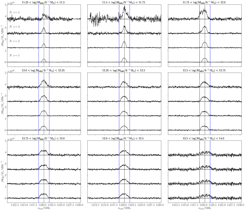
Figure 10: Stacks of group centrals divided into halo mass bins in separate panels. The vertical offset corresponds to the membership thresholds ranging from a minimum of 1 to 4 members (increasing upwards). The vertical blue dashed lines show the range the flux was integrated over to estimate the total Hi mass of the centrals in each stack.

However, although different halo properties are correlated with each other, the dependence of the total Hi gas mas on the different halo properties could potentially correspond to very different physical formation scenarios. It has previously been proposed that the Hi-rich galaxies tend to live in high-spin halos (e.g., Huang et al., 2012; Maddox et al., 2015; Obreschkow et al., 2016). For example, Lutz et al. (2018) used a sample of extremely Hi-rich galaxies and found a positive correlation between the gas ratio and the halo spin parameter. Galaxies in their sample have stellar masses in the range of $10^{10}M_{\sun}$–$10^{11}M_{\sun}$, which corresponds to a halo mass range around $10^{11.5}h^{-1}M_{\sun}$–$10^{12.5}h^{-1}M_{\sun}$ (Moster et al., 2010; Yang et al., 2012). If the Hi mass is indeed the indicator of the halo bias, the Hi mass would potentially have a much stronger dependence on the halo formation time than spin parameter in this mass range (see e.g., Fig. 4 of Sato-Polito et al., 2019). As shown in Figure 10 of Guo et al. (2017), the spin parameter is insufficient to explain the spatial clustering of the Hi-rich galaxies in the halo mass range of $10^{10}h^{-1}M_{\sun}$–$10^{12}h^{-1}M_{\sun}$.

The physical formation scenario of the Hi-rich galaxies is still under investigation. The Hi-rich galaxies can be formed from the recent gas accretion that increases the Hi reservoir, which is related to the halo formation time dependence. On the other hand, they can accrete their gas at an early time but the consumption of the cold Hi gas can be inefficient due to the high halo angular momentum that prevents the gas from collapsing and forming stars (Obreschkow et al., 2016; Lagos et al., 2018; Stevens et al., 2019). While both factors can be important in the real formation scenario, they can play different roles at different stages. From combining the dependence of Hi mass on the different halo properties, the plausible scenario is that in group halos of $M_{\rm h}<10^{13}h^{-1}M_{\sun}$, the recent gas accretion from the local halo environment is the dominant factor of the high Hi mass. This is also supported by the significant increase of total Hi mass in the satellite galaxies with the halo richness, as shown in Figure 3. As the spin parameters of these late-forming halos are also relatively higher, the transition from atomic to molecular hydrogen may be further hindered by the high angular momentum and the lack of enough disk pressure (Blitz & Rosolowsky, 2006; Popping et al., 2015; Lagos et al., 2017).

As shown in Figure 3, the growth of the total Hi mass is very efficient for halos of $M_{\rm h}<10^{11.8}h^{-1}M_{\sun}$, where the contribution from “cold mode” of the gas accretion is significant. As shown in Figure 6 of Kereš et al. (2005), the cold gas accretion becomes negligible in halos of $M_{\rm h}>10^{12}M_{\sun}$, consistent with our finding here. For more massive halos of $10^{11.8}h^{-1}M_{\sun}<M_{\rm h}<10^{13}h^{-1}M_{\sun}$, where the “hot mode” dominates, the supply of cold gas to the central galaxies is inefficient due to the virial shock-heating of the infalling gas (Birnboim & Dekel, 2003; Kereš et al., 2005; Dekel & Birnboim, 2006). Therefore, the dependence of central Hi mass on the halo richness becomes weaker in this halo mass range. We note that the exact transition halo mass scale between the cold and hot mode dominance would depend on the definition of cold flows and the simulation models, typically varying from $10^{11.4}M_{\sun}$ to $10^{12}M_{\sun}$ (Kereš et al., 2005; van de Voort et al., 2011; Correa et al., 2018).

However, as shown in Figure 13 of Kereš et al. (2005), the transition mass scale is also dependent on the local galaxy number density. At $z=0$, the cold mode dominates for $n_{\rm gal}<0.2\,h^{3}\rm{Mpc}^{-3}$, which corresponds to a halo richness of $1.3$ for $M_{\rm h}\sim 10^{12.5}h^{-1}M_{\sun}$. Therefore, our results in Figures 2 and 3 show that for halos with a richness smaller than 3, the cold mode accretion is important to the contribution of the Hi gas. As shown in the comparisons with the SAM of L-GALAXIES and the hydrodynamical simulations of Illustris and IllustrisTNG, where the virial shock-heating is included in the models, the effect of AGN feedback for halos of $M_{\rm h}>10^{12}h^{-1}M_{\sun}$ is necessary to match the observed Hi mass. The strong dependence of the satellite Hi mass on the halo richness indicates that cold gas accretion in the outer parts of the halo is not significantly affected by the AGN feedback.

For halos more massive than $10^{13}h^{-1}M_{\sun}$, the hot accretion mode is not efficient (Kereš et al., 2009) and the growth of halos is dominated by the mergers (see e.g., Fig. 5 of Genel et al., 2010). The halos with different formation times have similar large-scale environments, reflected by the insensitivity of halo bias on the formation time. The amount of accreted cold gas is then similar for these halos, manifested by the independence of Hi mass on the halo richness. As the effect of AGN feedback increases with the halo mass, the average cold gas mass of the central galaxy is then decreasing with the halo mass. The halo spin parameter would then potentially play a dominant role in determining the total Hi mass in these halos, as the consumption of Hi gas is lower for higher-spin halos.

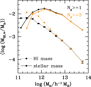
Figure 8: Comparisons between the gas fraction $M_{\rm HI}/M_{\rm h}$ (points with dotted lines) and the stellar mass fraction $M_{\ast}/M_{\rm h}$ (points with solid lines), for central galaxies in halos with $N_{\rm g}\geq 1$ (black lines) and $N_{\rm g}\geq 3$ (orange lines).

To study the connection between Hi gas and star formation, we show in Figure 8 the comparisons between the gas fraction $M_{\rm HI}/M_{\rm h}$ (points with dotted lines) and the stellar mass fraction $M_{\ast}/M_{\rm h}$ (points with solid lines), for central galaxies in halos with $N_{\rm g}\geq 1$ (black lines) and $N_{\rm g}\geq 3$ (orange lines). The peak of the gas fraction happens around $M_{\rm h}\sim 10^{11.5}h^{-1}M_{\sun}$, while that of the stellar mass fraction is at $M_{\rm h}\sim 10^{12.1}h^{-1}M_{\sun}$. It indicates that the AGN feedback starts to be effective from a halo mass of $10^{11.5}h^{-1}M_{\sun}$. While the gas fraction is decreasing with the halo mass from $10^{11.5}h^{-1}M_{\sun}$ to $10^{12}h^{-1}M_{\sun}$, the total Hi mass is still rapidly increasing through the smooth accretion up to $M_{\rm h}=10^{11.8}h^{-1}M_{\sun}$, where the virial shock-heating starts to heat the infalling gas (Dekel & Birnboim, 2006). The accretion of Hi gas in this halo mass range contributes to the increase of galaxy stellar mass before reaching the peak at $M_{\rm h}\sim 10^{12.1}h^{-1}M_{\sun}$. We note that the stellar mass fraction of halos with $N_{\rm g}\geq 3$ is slightly smaller than those with $N_{\rm g}\geq 1$. The late accretion of cold gas in the high-richness halos may cause less Hi gas to be converted into stars.

In summary, the formation scenario of the Hi-rich galaxies involves complicated physical processes. Both the halo mass and the halo formation history are important in the various processes. Further investigations in the semi-analytical models and the hydrodynamical simulations to reproduce the observed Hi-halo mass relation would help understand their formation and evolution.

6 Conclusions

In this paper, we have accurately measured the total Hi mass in halos of different masses by stacking Hi spectra of entire groups within the ALFALFA survey. Using the galaxy group catalog constructed from the optical survey of SDSS DR7, we are able to reliably determine both the halo mass and the halo membership, thereby constraining the Hi-halo mass relation for halos in a broad mass range from $10^{11}h^{-1}M_{\sun}$ to $10^{14}h^{-1}M_{\sun}$. It provides important constraints to the formation of the Hi-rich galaxies.

Our main conclusions are summarized as follows.

• Total Hi mass is not a single monotonically increasing function of halo mass. There is a bump in the function around $M_{\rm h}\sim 10^{12}h^{-1}M_{\sun}$.

• The contribution to the total Hi mass is dominated by the central galaxies for halos of $M_{\rm h}<10^{12}h^{-1}M_{\sun}$. Above this mass, satellites make the dominant contribution.

• The Hi mass of a halo is not only a function of halo mass. There is a significant secondary dependence on richness, with richer halos having higher Hi masses. This secondary dependence is strongest for low-mass halos and completely absent for the most massive halos.

• The bump in the Hi-halo mass relation is the result of a sharp dip in the Hi mass of centrals (in halos with $N_{\rm g}>=2$) at a halo mass of $M_{\rm h}\sim 10^{12}h^{-1}M_{\sun}$. The total Hi mass in satellite galaxies, on the other hand, monotonically increases with halo mass.

• We compare our measurements to the L-GALAXIES SAM and the hydrodynamical simulation models of Illustris and IllustrisTNG. We find that all of the models over-predict the abundance of Hi gas for halos of $M_{\rm h}>10^{11.5}h^{-1}M_{\sun}$. The drop of Hi mass in central galaxies is observed in different models with various levels. The strength of AGN feedback in the theoretical models is the key part to reproduce the observation.

• Our accurate measurements of the Hi-halo mass relation implies that the formation of the Hi gas in the halo can be divided into three phases. The smooth cold gas accretion is driving the growth of Hi mass in halos of $M_{\rm h}<10^{11.8}h^{-1}M_{\sun}$, with late-forming halos having more cold Hi gas accreted. The virial halo shock-heating and AGN feedback will reduce the cold gas supply in halos of $10^{11.8}h^{-1}M_{\sun}<M_{\rm h}<10^{13}h^{-1}M_{\sun}$. The Hi mass in halos more massive than $10^{13}h^{-1}M_{\sun}$ generally grows by mergers, where the dependence on halo richness and formation time becomes much weaker.

Table 1: Measurements of the Hi-halo mass relation

$\log M_{\rm h}$ range	$N_{\rm halo}$	$\langle\log M_{\rm HI}\rangle_{N_{\rm g}\geq 1}$	$\langle\log M_{\rm HI}\rangle_{N_{\rm g}\geq 2}$	$\langle\log M_{\rm HI}\rangle_{N_{\rm g}\geq 3}$	$\langle\log M_{\rm HI}\rangle_{N_{\rm g}\geq 4}$	$\langle\log M_{\rm HI}\rangle_{N_{\rm g}\geq 5}$	$\langle\log M_{\rm HI}\rangle_{N_{\rm g}\geq 6}$
$[11.0,11.25]$	949	$8.951\pm 0.020$	$9.167\pm 0.114$	$\cdots$	$\cdots$	$\cdots$	$\cdots$
$[11.25,11.5]$	3494	$9.239\pm 0.011$	$9.445\pm 0.036$	$9.626\pm 0.106$	$9.757\pm 0.320$	$\cdots$	$\cdots$
$[11.5,11.75]$	5472	$9.436\pm 0.008$	$9.660\pm 0.024$	$9.831\pm 0.070$	$10.046\pm 0.150$	$\cdots$	$\cdots$
$[11.75,12.0]$	7021	$9.467\pm 0.007$	$9.733\pm 0.016$	$9.918\pm 0.039$	$10.072\pm 0.081$	$9.869\pm 0.156$	$\cdots$
$[12.0,12.25]$	3903	$9.613\pm 0.010$	$9.798\pm 0.016$	$9.938\pm 0.029$	$10.009\pm 0.053$	$9.914\pm 0.094$	$10.074\pm 0.167$
$[12.25,12.5]$	2074	$9.708\pm 0.014$	$9.805\pm 0.018$	$9.914\pm 0.027$	$9.920\pm 0.041$	$10.047\pm 0.059$	$10.121\pm 0.088$
$[12.5,12.75]$	1375	$9.760\pm 0.017$	$9.858\pm 0.021$	$9.922\pm 0.026$	$10.001\pm 0.035$	$10.025\pm 0.047$	$10.099\pm 0.064$
$[12.75,13.0]$	803	$9.875\pm 0.022$	$9.941\pm 0.025$	$9.994\pm 0.028$	$10.078\pm 0.034$	$10.073\pm 0.042$	$10.170\pm 0.050$
$[13.0,13.5]$	646	$10.081\pm 0.024$	$10.104\pm 0.026$	$10.100\pm 0.027$	$10.117\pm 0.029$	$10.117\pm 0.032$	$10.124\pm 0.035$
$[13.5,14.0]$	147	$10.096\pm 0.050$	$10.165\pm 0.051$	$10.175\pm 0.051$	$10.180\pm 0.051$	$10.191\pm 0.052$	$10.170\pm 0.053$

Note. — Measurements of $\langle M_{\rm HI}|M_{\rm h}\rangle$ for halos with different richness $N_{\rm g}$. All masses are in units of $h^{-1}M_{\sun}$. The range of halo mass and total number of halos $N_{\rm halo}$ used in stacking of each mass bin for $N_{\rm g}\geq 1$ are also displayed.

Table 2: Measurements of the Hi-halo mass relation for central galaxies

$\log M_{\rm h}$ range	$\langle\log M_{\rm HI,cen}\rangle_{N_{\rm g}\geq 1}$	$\langle\log M_{\rm HI,cen}\rangle_{N_{\rm g}\geq 2}$	$\langle\log M_{\rm HI,cen}\rangle_{N_{\rm g}\geq 3}$	$\langle\log M_{\rm HI,cen}\rangle_{N_{\rm g}\geq 4}$	$\langle\log M_{\rm HI,cen}\rangle_{N_{\rm g}\geq 5}$	$\langle\log M_{\rm HI,cen}\rangle_{N_{\rm g}\geq 6}$
$[11.0,11.25]$	$8.936\pm 0.020$	$9.018\pm 0.114$	$\cdots$	$\cdots$	$\cdots$	$\cdots$
$[11.25,11.5]$	$9.200\pm 0.010$	$9.302\pm 0.036$	$9.440\pm 0.106$	$9.490\pm 0.320$	$\cdots$	$\cdots$
$[11.5,11.75]$	$9.402\pm 0.008$	$9.559\pm 0.024$	$9.652\pm 0.070$	$9.934\pm 0.150$	$\cdots$	$\cdots$
$[11.75,12.0]$	$9.450\pm 0.007$	$9.634\pm 0.016$	$9.771\pm 0.038$	$9.982\pm 0.080$	$9.666\pm 0.155$	$\cdots$
$[12.0,12.25]$	$9.550\pm 0.010$	$9.658\pm 0.015$	$9.742\pm 0.029$	$9.790\pm 0.053$	$9.734\pm 0.094$	$9.864\pm 0.167$
$[12.25,12.5]$	$9.612\pm 0.013$	$9.655\pm 0.018$	$9.704\pm 0.027$	$9.693\pm 0.041$	$9.769\pm 0.058$	$9.788\pm 0.087$
$[12.5,12.75]$	$9.649\pm 0.017$	$9.684\pm 0.021$	$9.702\pm 0.026$	$9.746\pm 0.035$	$9.774\pm 0.047$	$9.762\pm 0.064$
$[12.75,13.0]$	$9.709\pm 0.022$	$9.704\pm 0.025$	$9.721\pm 0.028$	$9.743\pm 0.034$	$9.723\pm 0.042$	$9.741\pm 0.050$
$[13.0,13.5]$	$9.722\pm 0.024$	$9.723\pm 0.026$	$9.725\pm 0.027$	$9.719\pm 0.029$	$9.723\pm 0.032$	$9.716\pm 0.035$
$[13.5,14.0]$	$9.632\pm 0.050$	$9.629\pm 0.051$	$9.634\pm 0.052$	$9.628\pm 0.052$	$9.623\pm 0.053$	$9.627\pm 0.053$

Note. — Similar to Table 1, but for the central galaxies.

Appendix A Measurements of Hi-halo mass relation

We list in Tables 1 and 2 the measurements of the Hi-halo mass relation for the halos and central galaxies, respectively. The number of halos in each mass bin used in the stacking is also displayed. We note that in the final stacking we only include part of the halos in each bin due to the effects of low S/N, failed spectra or overlapping with the survey boundary.

Appendix B Stacked Spectra

We show the stacked spectra for halos and central galaxies in Figures 9 and 10. We only show the results for halos in the mass range of $10^{11.25}$–$10^{14}h^{-1}M_{\sun}$, with different richness values from a minimum of one member to four members.

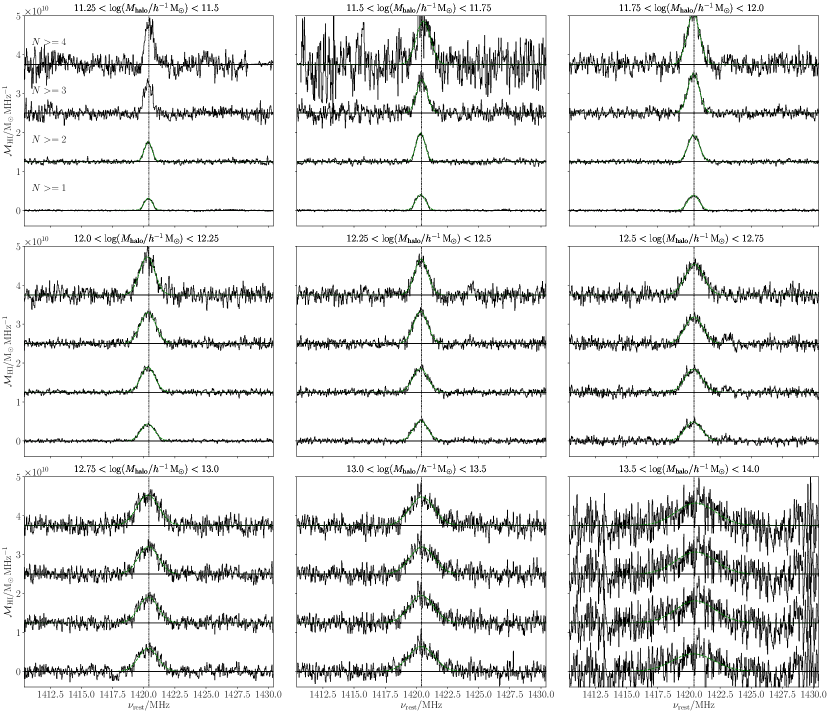
Figure 9: Stacks of groups divided into halo mass bins in separate panels. The vertical offset corresponds to the membership thresholds ranging from a minimum of one to four members (increasing upwards). The green dashed lines show the Gaussian fits to the profiles where appropriate.

References

- Ai & Zhu (2018) Ai, M., & Zhu, M. 2018, ApJ, 862, 48, doi: 10.3847/1538-4357/aac9b7
- Albareti et al. (2017) Albareti, F. D., Allende Prieto, C., Almeida, A., & et al. 2017, ApJS, 233, 25, doi: 10.3847/1538-4365/aa8992
- Barnes et al. (2001) Barnes, D. G., Staveley-Smith, L., de Blok, W. J. G., et al. 2001, MNRAS, 322, 486, doi: 10.1046/j.1365-8711.2001.04102.x
- Barnes & Haehnelt (2014) Barnes, L. A., & Haehnelt, M. G. 2014, MNRAS, 440, 2313, doi: 10.1093/mnras/stu445
- Baugh et al. (2019) Baugh, C. M., Gonzalez-Perez, V., Lagos, C. d. P., et al. 2019, MNRAS, 483, 4922, doi: 10.1093/mnras/sty3427
- Birnboim & Dekel (2003) Birnboim, Y., & Dekel, A. 2003, MNRAS, 345, 349, doi: 10.1046/j.1365-8711.2003.06955.x
- Blitz & Rosolowsky (2006) Blitz, L., & Rosolowsky, E. 2006, ApJ, 650, 933, doi: 10.1086/505417
- Brown et al. (2015) Brown, T., Catinella, B., Cortese, L., et al. 2015, MNRAS, 452, 2479, doi: 10.1093/mnras/stv1311
- Brown et al. (2017) —. 2017, MNRAS, 466, 1275, doi: 10.1093/mnras/stw2991
- Campbell et al. (2015) Campbell, D., van den Bosch, F. C., Hearin, A., et al. 2015, MNRAS, 452, 444, doi: 10.1093/mnras/stv1091
- Catinella et al. (2010) Catinella, B., Schiminovich, D., Kauffmann, G., et al. 2010, MNRAS, 403, 683, doi: 10.1111/j.1365-2966.2009.16180.x
- Correa et al. (2018) Correa, C. A., Schaye, J., Wyithe, J. S. B., et al. 2018, MNRAS, 473, 538, doi: 10.1093/mnras/stx2332
- Dekel & Birnboim (2006) Dekel, A., & Birnboim, Y. 2006, MNRAS, 368, 2, doi: 10.1111/j.1365-2966.2006.10145.x
- Delhaize et al. (2013) Delhaize, J., Meyer, M. J., Staveley-Smith, L., & Boyle, B. J. 2013, MNRAS, 433, 1398, doi: 10.1093/mnras/stt810
- Di Matteo et al. (2005) Di Matteo, T., Springel, V., & Hernquist, L. 2005, Nature, 433, 604, doi: 10.1038/nature03335
- Diemer et al. (2018) Diemer, B., Stevens, A. R. H., Forbes, J. C., et al. 2018, ApJS, 238, 33, doi: 10.3847/1538-4365/aae387
- Diemer et al. (2019) Diemer, B., Stevens, A. R. H., Lagos, C. d. P., et al. 2019, MNRAS, 487, 1529, doi: 10.1093/mnras/stz1323
- Fabello et al. (2011) Fabello, S., Catinella, B., Giovanelli, R., et al. 2011, MNRAS, 411, 993, doi: 10.1111/j.1365-2966.2010.17742.x
- Fabello et al. (2012) Fabello, S., Kauffmann, G., Catinella, B., et al. 2012, MNRAS, 427, 2841, doi: 10.1111/j.1365-2966.2012.22088.x
- Fu et al. (2013) Fu, J., Kauffmann, G., Huang, M.-l., et al. 2013, MNRAS, 434, 1531, doi: 10.1093/mnras/stt1117
- Gao et al. (2005) Gao, L., Springel, V., & White, S. D. M. 2005, MNRAS, 363, L66, doi: 10.1111/j.1745-3933.2005.00084.x
- Gao & White (2007) Gao, L., & White, S. D. M. 2007, MNRAS, 377, L5, doi: 10.1111/j.1745-3933.2007.00292.x
- Genel et al. (2010) Genel, S., Bouché, N., Naab, T., Sternberg, A., & Genzel, R. 2010, ApJ, 719, 229, doi: 10.1088/0004-637X/719/1/229
- Geréb et al. (2015) Geréb, K., Morganti, R., Oosterloo, T. A., Hoppmann, L., & Staveley-Smith, L. 2015, A&A, 580, A43, doi: 10.1051/0004-6361/201424810
- Giovanelli et al. (2005) Giovanelli, R., Haynes, M. P., Kent, B. R., et al. 2005, AJ, 130, 2598, doi: 10.1086/497431
- Guo et al. (2017) Guo, H., Li, C., Zheng, Z., et al. 2017, ApJ, 846, 61, doi: 10.3847/1538-4357/aa85e7
- Guo et al. (2015) Guo, H., Zheng, Z., Zehavi, I., et al. 2015, MNRAS, 453, 4368, doi: 10.1093/mnras/stv1966
- Haynes et al. (2011) Haynes, M. P., Giovanelli, R., Martin, A. M., et al. 2011, AJ, 142, 170, doi: 10.1088/0004-6256/142/5/170
- Haynes et al. (2018) Haynes, M. P., Giovanelli, R., Kent, B. R., et al. 2018, ApJ, 861, 49, doi: 10.3847/1538-4357/aac956
- Helfer et al. (2003) Helfer, T. T., Thornley, M. D., Regan, M. W., et al. 2003, ApJS, 145, 259, doi: 10.1086/346076
- Hu et al. (2019) Hu, W., Hoppmann, L., Staveley-Smith, L., et al. 2019, MNRAS, 489, 1619, doi: 10.1093/mnras/stz2038
- Huang et al. (2012) Huang, S., Haynes, M. P., Giovanelli, R., & Brinchmann, J. 2012, ApJ, 756, 113, doi: 10.1088/0004-637X/756/2/113
- Jing et al. (2007) Jing, Y. P., Suto, Y., & Mo, H. J. 2007, ApJ, 657, 664, doi: 10.1086/511130
- Jones et al. (2018) Jones, M. G., Haynes, M. P., Giovanelli, R., & Moorman, C. 2018, MNRAS, 477, 2, doi: 10.1093/mnras/sty521
- Jones et al. (2020) Jones, M. G., Hess, K. M., Adams, E. A. K., & Verdes-Montenegro, L. 2020, arXiv e-prints, arXiv:2003.09302. https://arxiv.org/abs/2003.09302
- Kereš et al. (2009) Kereš, D., Katz, N., Fardal, M., Davé, R., & Weinberg, D. H. 2009, MNRAS, 395, 160, doi: 10.1111/j.1365-2966.2009.14541.x
- Kereš et al. (2005) Kereš, D., Katz, N., Weinberg, D. H., & Davé, R. 2005, MNRAS, 363, 2, doi: 10.1111/j.1365-2966.2005.09451.x
- Kim et al. (2017) Kim, H.-S., Wyithe, J. S. B., Baugh, C. M., et al. 2017, MNRAS, 465, 111, doi: 10.1093/mnras/stw2779
- Krumholz (2013) Krumholz, M. R. 2013, MNRAS, 436, 2747, doi: 10.1093/mnras/stt1780
- Lagos et al. (2017) Lagos, C. d. P., Theuns, T., Stevens, A. R. H., et al. 2017, MNRAS, 464, 3850, doi: 10.1093/mnras/stw2610
- Lagos et al. (2018) Lagos, C. d. P., Tobar, R. J., Robotham, A. S. G., et al. 2018, MNRAS, 481, 3573, doi: 10.1093/mnras/sty2440
- Lah et al. (2007) Lah, P., Chengalur, J. N., Briggs, F. H., et al. 2007, MNRAS, 376, 1357, doi: 10.1111/j.1365-2966.2007.11540.x
- Leroy et al. (2009) Leroy, A. K., Walter, F., Bigiel, F., et al. 2009, AJ, 137, 4670, doi: 10.1088/0004-6256/137/6/4670
- Li et al. (2012) Li, C., Kauffmann, G., Fu, J., et al. 2012, MNRAS, 424, 1471, doi: 10.1111/j.1365-2966.2012.21337.x
- Li & White (2009) Li, C., & White, S. D. M. 2009, MNRAS, 398, 2177, doi: 10.1111/j.1365-2966.2009.15268.x
- Lim et al. (2017) Lim, S. H., Mo, H. J., Lu, Y., Wang, H., & Yang, X. 2017, MNRAS, 470, 2982, doi: 10.1093/mnras/stx1462
- Lutz et al. (2018) Lutz, K. A., Kilborn, V. A., Koribalski, B. S., et al. 2018, MNRAS, 476, 3744, doi: 10.1093/mnras/sty387
- Maddox et al. (2015) Maddox, N., Hess, K. M., Obreschkow, D., Jarvis, M. J., & Blyth, S. L. 2015, MNRAS, 447, 1610, doi: 10.1093/mnras/stu2532
- Man & Belli (2018) Man, A., & Belli, S. 2018, Nature Astronomy, 2, 695, doi: 10.1038/s41550-018-0558-1
- Marinacci et al. (2018) Marinacci, F., Vogelsberger, M., Pakmor, R., et al. 2018, MNRAS, 480, 5113, doi: 10.1093/mnras/sty2206
- Martin et al. (2010) Martin, A. M., Papastergis, E., Giovanelli, R., et al. 2010, ApJ, 723, 1359, doi: 10.1088/0004-637X/723/2/1359
- Meyer et al. (2017) Meyer, M., Robotham, A., Obreschkow, D., et al. 2017, PASA, 34, 52, doi: 10.1017/pasa.2017.31
- Meyer et al. (2004) Meyer, M. J., Zwaan, M. A., Webster, R. L., et al. 2004, MNRAS, 350, 1195, doi: 10.1111/j.1365-2966.2004.07710.x
- Moster et al. (2010) Moster, B. P., Somerville, R. S., Maulbetsch, C., et al. 2010, ApJ, 710, 903, doi: 10.1088/0004-637X/710/2/903
- Naiman et al. (2018) Naiman, J. P., Pillepich, A., Springel, V., et al. 2018, MNRAS, 477, 1206, doi: 10.1093/mnras/sty618
- Nelson et al. (2018) Nelson, D., Pillepich, A., Springel, V., et al. 2018, MNRAS, 475, 624, doi: 10.1093/mnras/stx3040
- Obreschkow et al. (2016) Obreschkow, D., Glazebrook, K., Kilborn, V., & Lutz, K. 2016, ApJ, 824, L26, doi: 10.3847/2041-8205/824/2/L26
- Obuljen et al. (2019) Obuljen, A., Alonso, D., Villaescusa-Navarro, F., Yoon, I., & Jones, M. 2019, MNRAS, 486, 5124, doi: 10.1093/mnras/stz1118
- Papastergis et al. (2011) Papastergis, E., Martin, A. M., Giovanelli, R., & Haynes, M. P. 2011, ApJ, 739, 38, doi: 10.1088/0004-637X/739/1/38
- Paul et al. (2018) Paul, N., Choudhury, T. R., & Paranjape, A. 2018, MNRAS, 479, 1627, doi: 10.1093/mnras/sty1539
- Pillepich et al. (2018) Pillepich, A., Nelson, D., Hernquist, L., et al. 2018, MNRAS, 475, 648, doi: 10.1093/mnras/stx3112
- Planck Collaboration et al. (2014) Planck Collaboration, Ade, P. A. R., Aghanim, N., & et al. 2014, A&A, 571, A16, doi: 10.1051/0004-6361/201321591
- Popping et al. (2015) Popping, G., Behroozi, P. S., & Peeples, M. S. 2015, MNRAS, 449, 477, doi: 10.1093/mnras/stv318
- Rees & Ostriker (1977) Rees, M. J., & Ostriker, J. P. 1977, MNRAS, 179, 541, doi: 10.1093/mnras/179.4.541
- Rhee et al. (2013) Rhee, J., Zwaan, M. A., Briggs, F. H., et al. 2013, MNRAS, 435, 2693, doi: 10.1093/mnras/stt1481
- Saintonge et al. (2011) Saintonge, A., Kauffmann, G., Kramer, C., et al. 2011, MNRAS, 415, 32, doi: 10.1111/j.1365-2966.2011.18677.x
- Saintonge et al. (2018) Saintonge, A., Wilson, C. D., Xiao, T., et al. 2018, MNRAS, 481, 3497, doi: 10.1093/mnras/sty2499
- Sato-Polito et al. (2019) Sato-Polito, G., Montero-Dorta, A. D., Abramo, L. R., Prada, F., & Klypin, A. 2019, MNRAS, 487, 1570, doi: 10.1093/mnras/stz1338
- Silk (1977) Silk, J. 1977, ApJ, 211, 638, doi: 10.1086/154972
- Springel et al. (2018) Springel, V., Pakmor, R., Pillepich, A., et al. 2018, MNRAS, 475, 676, doi: 10.1093/mnras/stx3304
- Stevens et al. (2019) Stevens, A. R. H., Diemer, B., Lagos, C. d. P., et al. 2019, MNRAS, 483, 5334, doi: 10.1093/mnras/sty3451
- van de Voort et al. (2011) van de Voort, F., Schaye, J., Booth, C. M., Haas, M. R., & Dalla Vecchia, C. 2011, MNRAS, 414, 2458, doi: 10.1111/j.1365-2966.2011.18565.x
- Verheijen et al. (2007) Verheijen, M., van Gorkom, J. H., Szomoru, A., et al. 2007, ApJ, 668, L9, doi: 10.1086/522621
- Villaescusa-Navarro et al. (2018) Villaescusa-Navarro, F., Genel, S., Castorina, E., et al. 2018, ApJ, 866, 135, doi: 10.3847/1538-4357/aadba0
- Vogelsberger et al. (2014) Vogelsberger, M., Genel, S., Springel, V., et al. 2014, MNRAS, 444, 1518, doi: 10.1093/mnras/stu1536
- Wang et al. (2016) Wang, J., Koribalski, B. S., Serra, P., et al. 2016, MNRAS, 460, 2143, doi: 10.1093/mnras/stw1099
- Wechsler et al. (2006) Wechsler, R. H., Zentner, A. R., Bullock, J. S., Kravtsov, A. V., & Allgood, B. 2006, ApJ, 652, 71, doi: 10.1086/507120
- White & Rees (1978) White, S. D. M., & Rees, M. J. 1978, MNRAS, 183, 341, doi: 10.1093/mnras/183.3.341
- Wolz et al. (2019) Wolz, L., Murray, S. G., Blake, C., & Wyithe, J. S. 2019, MNRAS, 484, 1007, doi: 10.1093/mnras/sty3142
- Xu & Zheng (2018) Xu, X., & Zheng, Z. 2018, MNRAS, 479, 1579, doi: 10.1093/mnras/sty1547
- Yang et al. (2007) Yang, X., Mo, H. J., van den Bosch, F. C., et al. 2007, ApJ, 671, 153, doi: 10.1086/522027
- Yang et al. (2012) Yang, X., Mo, H. J., van den Bosch, F. C., Zhang, Y., & Han, J. 2012, ApJ, 752, 41, doi: 10.1088/0004-637X/752/1/41
- York et al. (2000) York, D. G., Adelman, J., Anderson, Jr., J. E., et al. 2000, AJ, 120, 1579, doi: 10.1086/301513
- Zhang et al. (2009) Zhang, W., Li, C., Kauffmann, G., et al. 2009, MNRAS, 397, 1243, doi: 10.1111/j.1365-2966.2009.15050.x
- Zoldan et al. (2017) Zoldan, A., De Lucia, G., Xie, L., Fontanot, F., & Hirschmann, M. 2017, MNRAS, 465, 2236, doi: 10.1093/mnras/stw2901