Evolution of the Thermodynamic Properties of Clusters of Galaxies out to Redshift of 1.8

Abstract

The thermodynamic properties of the hot plasma in galaxy clusters retains information on the processes leading to the formation and evolution of the gas in their deep, dark matter potential wells. These processes are dictated not only by gravity but also by gas physics, e.g. AGN feedback and turbulence. In this work, we study the thermodynamic properties, e.g. density, temperature, pressure, and entropy, of the most massive and the most distant ($z>1.2$) SPT-selected clusters, and compare them with those of the nearby clusters ($z<0.1$) to constrain their evolution as a function of time and radius. We find that thermodynamic properties in the outskirts of high redshift clusters are remarkably similar to the low redshift clusters, and their evolution follows the prediction of the self-similar model. Their intrinsic scatter is larger, indicating that the physical properties that lead to the formation and virialization of cluster outskirts show evolving variance. On the other hand, thermodynamic properties in the cluster cores deviates significantly from self-similarity indicating that the processes that regulate the core are already in place in these very high redshift clusters. This result is supported by the unevolving physical scatter of all thermodynamic quantities in cluster cores.

1 Introduction

Clusters of galaxies are the largest gravitationally-bound objects in the Universe and are ideal laboratories to study how cosmic structures form and evolve in time. While the majority of their mass is in the form of dark matter, the hot fully ionized plasma, i.e. the intra-cluster medium (ICM), retains most of the baryonic component, with only a small contribution from stars and cold gas (3-5%; Gonzalez et al., 2013). The ICM is observable in the X-ray band mainly through its emission via thermal Bremsstrahlung and radiative recombination processes. X-ray observations of clusters of galaxies provide in depth information about the ICM’s thermodynamic properties. The thermal Sunyaev-Zeldovich (SZ) effect, a spectral distortion of the cosmic microwave background caused by the ICM, provides a complementary tool for finding clusters at all redshifts and examining their properties.

X-ray studies of clusters of galaxies provided constraints on thermodynamic properties of the ICM in nearby clusters with redshifts of $<$0.3 (e.g. Croston et al., 2006; De Grandi & Molendi, 2002; Cavagnolo et al., 2009; Vikhlinin et al., 2006; Arnaud et al., 2010; Pratt et al., 2010; Bulbul et al., 2012). X-ray observations have also provided the serendipitous detection of single high redshift clusters ($z>1$; Fabian et al., 2003; Tozzi et al., 2015; Brodwin et al., 2016), however these studies are prone to X-ray selection biases (e.g. the cool-core bias, Eckert et al., 2011). The majority of theoretical studies in the literature also focus on predicting thermodynamic properties of the ICM in nearby clusters (Kravtsov & Borgani, 2012). In recent years, owing to the wide area sky surveys performed with the current SZ telescopes, e.g. the South Pole Telescope (SPT; Carlstrom et al., 2011), the Atacama Cosmology Telescope (Fowler et al., 2007), and the Planck mission (Planck Collaboration et al., 2016), it has become possible to detect clusters out to much higher redshifts (z$\sim$1.8) with a simpler selection function, i.e., the SZ signal tightly correlates with mass (Planck Collaboration et al., 2014; Bocquet et al., 2019). Therefore, X-ray follow-up observations of the SZ selected clusters provide a unique opportunity to study the evolution of ICM properties in a uniform way.

Integrated X-ray properties of the SPT-selected clusters spanning a large redshift range have been studied in the literature (McDonald et al., 2014; Sanders et al., 2018; Bulbul et al., 2019). Bartalucci et al. (2017a, b) examined the electron number density distribution of the ICM by combining the Chandra and XMM-Newton follow-up observations of a handful of high redshift clusters (z $\sim\,$ 1) detected by SPT and ACT. Studies of the evolution of the ICM properties in large SZ-selected cluster samples have become possible with large targeted X-ray follow-up programs, e.g. Chandra Large Program (LP). McDonald et al. (2013, 2014) have reported that the evolution in the electron number density is consistent with the self-similar expectation, where only gravitational forces dominate the formation and evolution of the ICM in the intermediate regions ($0.15R_{500}\,-\,R_{500}$) of the SPT-selected clusters of galaxies in the redshift range of $0.2<z<1.2$. The authors also found a clear deviation from self-similarity in the evolution of the core density of these clusters. Deeper Chandra observations of 8 high redshift SPT-selected clusters beyond redshift of 1.2 confirm earlier results of no evolution in the cluster cores indicating that Active Galactic Nuclei (AGN) feedback is tightly regulated since this early epoch and self-similar evolution is followed in intermediate regions (McDonald et al., 2017, hereafter MD17). Recently, Sanders et al. (2018) reported a self-similar evolution of the thermodynamic properties at all radii for the same large sample but using a different center and a slightly different analysis scheme out to $R_{500}$.

In this work, we combine deep Chandra and XMM-Newton observations of a sample of the highest redshift and most massive 7 SPT-selected galaxy clusters beyond redshift of 1.2 to study the thermodynamic properties of the ICM and their evolution. We take advantage of the sharp point spread function (PSF) of Chandra to study the small scales (at this redshift,beyond 1.2, Chandra resolution of 0.5 arcsec corresponds to about 5 kpc), while the large effective area of XMM-Newton provides the required photon statistics to measure densities and temperatures out to large scales. Thus, the combination of Chandra and XMM-Newton allows us to obtain precise and extended density profiles, and sufficient photon statistics to measure temperature profiles required to probe the evolution of the ICM properties, e.g. density, temperature, pressure, and entropy, out to the overdensity radius $R_{500}$. The paper is organized as follows: in Sect. 2, we present the sample properties and the analysis of the XMM-Newton and Chandra data of the sample; in Sect. 3 we provide our results; the systematic uncertainties are discussed in Sect. 4 and we finally summarize our conclusions in Sect. 5.

Throughout the paper we assume a flat $\Lambda$CDM cosmology with $\Omega_{m}=0.3$, $\Omega_{\Lambda}=0.7$ and $H_{0}=70$ km s^-1 Mpc^-1. All uncertainties quoted correspond to 68% single-parameter confidence intervals unless otherwise stated.

Cluster	redshift	R.A.	Dec.	tCXO	$t_{MOS1}$	$t_{MOS2}$	$t_{pn}$
		[deg]	[deg]	[ks]	[ks]	[ks]	[ks]
SPT-CLJ0205-5829	1.322	31.4437	-58.4855	57.8	69.4	70.2	52.7
SPT-CLJ0313-5334	1.474	48.4809	-53.5781	113.6	186.0	195.2	164.5
SPT-CLJ0459-4947	1.70	74.9269	-49.7872	136.2	461.9	471.6	410.3
SPT-CLJ0607-4448	1.401	91.8984	-44.8033	111.1	132.7	144.8	98.7
SPT-CLJ0640-5113	1.316	100.0645	-51.2204	173.4	127.7	131.9	114.0
SPT-CLJ2040-4451	1.478	310.2468	-44.8599	96.7	76.2	76.6	72.8
SPT-CLJ2341-5724	1.259	355.3568	-57.4158	112.4	107.7	107.7	93.0

Table 1: Properties of the sample; cluster name, redshift, coordinates of the centroid, Chandra clean exposure time, and XMM-Newton (EPIC MOS1, MOS2, and pn) clean exposure times.

2 Cluster Sample and Data analysis

2.1 Cluster Sample

Our sample consists of 7 SPT-selected high redshift ($z>1.2$) massive clusters of galaxies with S/N ratio greater than 6 and a total SZ inferred mass greater than $3\times 10^{14}\ M_{\odot}$ (Bleem et al., 2015). The deep XMM-Newton observations of these clusters have been performed in AO-16 (PIs E. Bulbul, and A. Mantz) and Chandra observations were performed in AO-16 through both XVP program (PI M. McDonald) and two guest observer (GO) programs (PI G. Garmire, S. Murray). The total Chandra and XMM-Newton clean exposure time used in this work is $\sim$2 Ms (see Table 1).

2.2 Imaging Analysis

2.2.1 XMM-Newton Imaging Analysis

We strictly follow the data analysis prescription developed by the XMM-Newton Cluster Outskirts Project collaboration (X-COP, Eckert et al., 2017) with their new background modeling method (Ghirardini et al., 2018a). Thanks to the reduction of the systematic uncertainty on the background below 5% through this method, we are able to measure thermodynamic properties of high redshift clusters out to $R_{500}$. We provide the summary of the analysis below. We use the XMM-Newton Science Analysis System (SAS) and Extended Source Analysis Software (ESAS, Snowden et al., 2008), developed to analyze XMM-Newton EPIC observations. In our analysis, we use XMM-SAS v17.0 and CALDB files as of January 2019 (XMM-CCF-REL-362).

Filtered event files are generated using the XMM-SAS tasks mos-filter and pn-filter. The photon count images are extracted from the filtered event files from three EPIC detectors, MOS1, MOS2, and pn on board XMM-Newton, in the soft and narrow energy band [0.7-1.2] keV. The choice of this narrow band is to maximize the source to background ratio and minimize the systematic uncertainties in the modeling of the EPIC background (Ettori & Molendi, 2011). To create the total EPIC images, the count images from the three detectors are summed. Next, we use eexpmap to compute exposure maps by also taking the vignetting effect into account. The exposure maps are also summed using the scaling factors of 1:1:3.44 for MOS1:MOS2:pn detectors, i.e. the ratio between the effective area of MOS and pn in the [0.7-1.2] keV energy band. These scaling factors are computed individually for each observation.

The high-energy particle background images are generated using the background images extracted from the unexposed corners of the detectors, and rescaling them to the field-of-view (FoV). After the light curve cleaning, residual soft protons still contaminate the FoV (Salvetti et al., 2017). We measure the soft proton contamination in the FoV of each observation by calculating the fraction of count rates in the unexposed and exposed portions of the detector in a hard band ([7–11.5] keV) (Leccardi & Molendi, 2008). We then generate the 2D soft proton image (Ghirardini et al., 2018a, as described in their Appendix A), to model the remaining soft proton contamination. We construct the total non-X-ray background (NXB) by summing the high energy particle background and the residual soft protons images. Thus, we obtain total photon images, exposure maps, and total non-X-ray background images for each observation.

To detect and excise point and extended sources in the FoV, we use the XMM-SAS tool ewavelet with a selection of scales in the range 1–32 pixels with S/N threshold of 5. We remove all the point sources found by ewavelet tool from the further analysis. We also run CIAO point source detection tool wavdetect on Chandra images. The sources detected on XMM-Newton and Chandra images are combined to remove missed point sources by ewavelet. See Sect. 2.2.3 for details on the Chandra analysis.

2.2.2 Point Spread Function Correction for XMM-Newton

Due to the relatively large size of the Point Spread Function (PSF) of XMM-Newton, some X-ray photons that originate from one particular region on the sky may be detected elsewhere on the detector. XMM-Newton’s 5 arcsec wide PSF (at aim point) needs to be taken into account to correct for this effect due to the small spatial scales of the clusters in our sample (Read et al., 2011). To estimate the impact of the PSF on surface brightness profiles, we first create a matrix, $PSF_{i,j}$, whose value is the fraction of photons originating in the i${}^{\text{th}}$ annulus in the sky but detected in the j${}^{\text{th}}$ annulus on the detector.

In practice, to model the PSF and build the PSF matrix, we, following Eckert et al. (2016) and (2019), build an image of an annulus with a constant value inside the annulus itself and zero outside, with the constant chosen in such a way that the sum of all pixels is 1; this represents the probability density function (PDF) for the true photons generated in the annulus that represents their origin on the plane of the sky. The XMM-Newton mirrors smear this annulus-limited PDF onto a larger fraction of the exposed CCDs. We then use a functional form (e.g., a King profile plus a Gaussian as in Read et al., 2011) to model the instrumental PSF function in each location of the detector. The observed photons are the result of the convolution of the original sky photons by the PSF function, $S_{\rm b,obs}={\rm PSF}\circledast S_{\rm b,true}$. The PDF is no longer limited to the annulus, but has spread to the surroundings. The fraction of the PDF, originating from annulus ‘$i$’, that now is present in annulus ‘$j$’ is the value that we put in the corresponding line and row of the PSF matrix. An example image of the PSF matrix is given in Figure 1. While the majority of the photons which originate from a given annulus are detected in the same region (the largest values are on the diagonal), some fraction of them are detected in a different annuli.

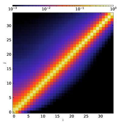
Figure 1: Example PSF matrix image used in our analysis. The matrix shows the contribution to the j^th annulus from the i^th annulus at each position $(i,j)$. The non-diagonal and asymmetric nature of the distribution shows that the contribution of the emission from the cluster center to the outskirts is not negligible and should be corrected for.

2.2.3 Chandra Imaging Analysis

We process the Chandra observations of the sample using the CIAO 4.11 (Chandra Interactive Analysis of Observations, Fruscione et al., 2006) and calibration files in CALDB 4.8.2. We filter the data for good time intervals, including the corrections for charge transfer inefficiency (Grant et al., 2005). We remove the photons detected in bad CCD columns and hot pixels, compute the calibrated photon energies by applying the ACIS gain maps, and correct for their time dependence. We also remove the time intervals that are affected by the background flares by examining the light curves. We ran wavdetect, the standard CIAO tool to find point sources in Chandra observations, with scales in range 1-32 pixels and threshold for identifying a pixel as belonging to a source of $10^{-6}$. We merge point sources detected on Chandra images with those detected on XMM-Newton images as described in Sect. 2.2.1. All point sources detected in this process are excluded from further analysis.

We extract photon count images in the soft energy band [0.5-2.0] keV, as it is routinely done when analyzing Chandra data.

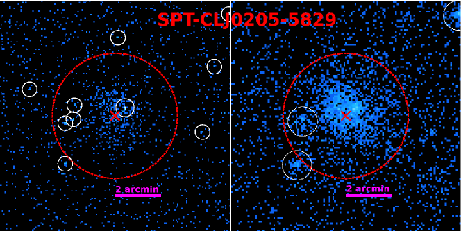
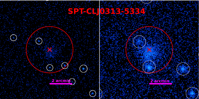
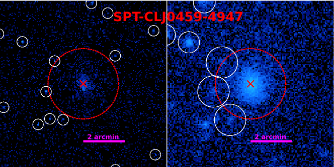
Figure 12: Raw count images of the clusters, Chandra counts are shown on the left, while the XMM-Newton image is shown on the right. The blue cross indicates the location of the center used, and the white circles indicate the point sources masked.

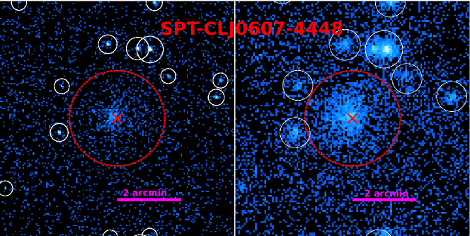
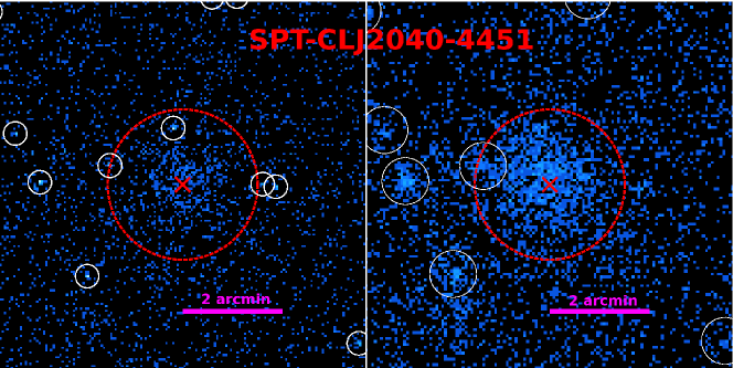
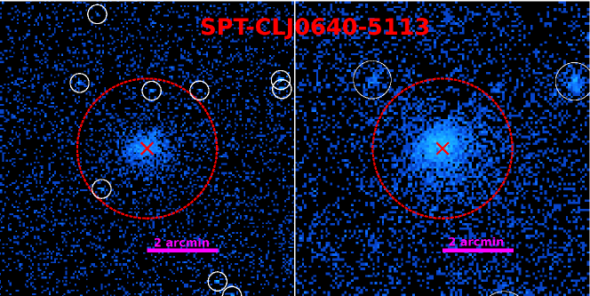
Figure 12: Continued

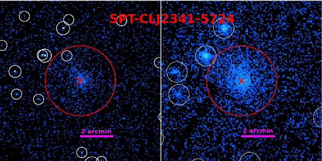
Figure 12: Continued

For the instrumental background we use blank-sky background spectra which is rescaled based on the flux in the hard band [9.5 - 12] keV to account for variations in the particle background. Exposure maps are generated to correct for vignetting effect. The particle background subtracted, vignetting corrected images are shown in Figure 12. Due to the small size of Chandra’s PSF, 80% of the total encircled counts are detected within 0.7 arcsec from its source. We, therefore, do not apply any PSF correction to Chandra data.

2.2.4 Joint Chandra  and XMM-Newton Surface Brightness Analysis

To compute the surface brightness profile, we first measure the number of photon counts ($N_{c,i}$) in concentric annuli around the cluster center. We find the cluster center by measuring the centroid in a 250–500 kpc aperture on Chandra images following the approach introduced by McDonald et al. (2013). This method allows us to find the center of the large scale distribution of the intra-cluster plasma independent of the core morphology. The widths of the annuli are required to be larger than 2 arcsec, increasing logarithmically, and with at least 30 counts contained within each annulus. For XMM-Newton the width of these annuli is determined in such way that each has at least a total of 100 counts and the minimum width is larger than 5 arcsec. We then compute the mean exposure time $t_{exp,i}$ from the exposure map, and background counts using the total background map $N_{\rm NXB,i}$ for the two X-ray telescopes. The surface brightness in each annulus is calculated using the following relation:

$$S_{B_{i}}=\frac{N_{\rm c,i}-N_{\rm NXB,i}}{t_{\rm exp,i}\cdot A_{\rm reg,i}}$$ (1)

where $A_{reg,i}$ is the area, in arcmin², of each annulus ‘$i$’.

Cluster	$\log(n_{0})$	$\log(r_{c})$	$\log(r_{s})$	$\alpha$	$\beta$	$\epsilon$	$\log(B_{XMM})$	$\log(B_{Chandra})$
SPT-CLJ0205-5829	$-4.87\pm 0.28$	$2.06\pm 0.45$	$5.62\pm 0.09$	$1.06\pm 0.48$	$-0.00\pm 0.04$	$6.17\pm 0.35$	$-10.99\pm 0.02$	$-10.81\pm 0.02$
SPT-CLJ0313-5334	$-4.83\pm 0.32$	$1.21\pm 0.78$	$5.62\pm 0.08$	$1.42\pm 0.95$	$0.03\pm 0.03$	$7.02\pm 0.51$	$-11.07\pm 0.02$	$-10.48\pm 0.01$
SPT-CLJ0459-4947	$-3.12\pm 0.15$	$2.08\pm 0.24$	$5.28\pm 0.09$	$1.09\pm 0.46$	$0.16\pm 0.03$	$4.69\pm 0.22$	$-10.78\pm 0.00$	$-10.09\pm 0.01$
SPT-CLJ0607-4448	$-3.16\pm 0.22$	$2.27\pm 0.29$	$5.16\pm 0.24$	$1.61\pm 0.45$	$0.20\pm 0.05$	$3.18\pm 0.21$	$-10.53\pm 0.01$	$-10.18\pm 0.01$
SPT-CLJ0640-5113	$-3.66\pm 0.20$	$2.02\pm 0.39$	$5.12\pm 0.10$	$1.21\pm 0.47$	$0.10\pm 0.03$	$4.31\pm 0.19$	$-10.78\pm 0.01$	$-10.38\pm 0.01$
SPT-CLJ2040-4451	$-5.21\pm 0.32$	$1.79\pm 0.45$	$5.75\pm 0.11$	$0.50\pm 0.47$	$0.01\pm 0.04$	$5.49\pm 0.34$	$-10.39\pm 0.01$	$-10.45\pm 0.02$
SPT-CLJ2341-5724	$-3.26\pm 0.09$	$2.72\pm 0.10$	$5.95\pm 0.10$	$0.45\pm 0.38$	$0.29\pm 0.01$	$3.24\pm 0.24$	$-10.48\pm 0.01$	$-10.61\pm 0.01$

Table 2: Best-fit parameters of the Vikhlinin et al. (2006) density model and measured background levels in the Chandra and XMM-Newton observations are given.

Cluster	$T_{0}$	$r_{cool}$	$r_{t}$	$\frac{T_{min}}{T_{0}}$	$a_{cool}$	$\frac{c}{2}$
	keV	kpc	kpc
SPT-CLJ0205-5829	$9.1\pm 2.2$	$23\pm 14$	$358\pm 195$	$0.45\pm 0.19$	$1.89\pm 0.51$	$0.36\pm 0.18$
SPT-CLJ0313-5334	$6.8\pm 1.5$	$24\pm 15$	$354\pm 184$	$0.44\pm 0.19$	$1.87\pm 0.51$	$0.40\pm 0.18$
SPT-CLJ0459-4947	$9.4\pm 1.3$	$22\pm 12$	$283\pm 112$	$0.46\pm 0.19$	$1.91\pm 0.50$	$0.44\pm 0.14$
SPT-CLJ0607-4448	$5.9\pm 0.8$	$25\pm 16$	$406\pm 225$	$0.44\pm 0.19$	$1.85\pm 0.50$	$0.28\pm 0.18$
SPT-CLJ0640-5113	$8.1\pm 1.4$	$23\pm 13$	$300\pm 136$	$0.45\pm 0.19$	$1.90\pm 0.51$	$0.45\pm 0.16$
SPT-CLJ2040-4451	$13.7\pm 4.2$	$22\pm 13$	$189\pm 71$	$0.46\pm 0.19$	$1.92\pm 0.50$	$0.62\pm 0.14$
SPT-CLJ2341-5724	$6.4\pm 1.0$	$23\pm 14$	$402\pm 220$	$0.44\pm 0.19$	$1.87\pm 0.51$	$0.30\pm 0.18$

Table 3: Best-fit parameters of the Vikhlinin et al. (2006) temperature model.

From a theoretical point of view, the surface brightness profile is related to the number density through;

$$S_{B_{i}}\propto n_{p}(r)\,n_{e}(r)\,dl$$ (2)

where $n_{p}$ and $n_{e}$ are number densities of protons and electrons, and $dl$ is the integral along the line of sight. We fit the Vikhlinin et al. (2006) density model to the observed Chandra and XMM-Newton surface brightness data, jointly.

$$n_{e}^{2}(r)=\frac{n_{0}^{2}\left(\frac{r}{r_{c}}\right)^{-\alpha}}{\left(1+\left(\frac{r}{r_{c}}\right)^{2}\right)^{3\beta-\alpha/2}\cdot\left(1+\left(\frac{r}{r_{s}}\right)^{3}\right)^{\epsilon/3}}$$ (3)

The parameters of the ICM model are constrained by fitting the observed counts $N_{c,i}$ in each annulus against the predicted counts $\mu_{i}$ (see Equation 5) using the following Poisson likelihood:

$$-\log\mathcal{L}=\sum_{i=1}^{N}\mu_{i}-N_{c,i}\log\mu_{i}$$ (4)

The net number of counts $\mu_{i}$ inferred by the ICM model in the $i$th annulus is calculated using the predicted surface brightness, Eq. 2, convolved with the PSF matrix, considering the exposed area and time for each annulus, as well as both sky and particle background.

$$\mu_{i}=\left\{\sum_{j}{\rm PSF}_{i,j}\cdot\left(S_{\rm b,ICM,i}+{\rm B_{sky}}\right)\right\}\cdot t_{\rm exp,i}\cdot A_{\rm reg,i}+N_{\rm NXB,i}$$ (5)

where $t_{\rm exp,i}$ and $A_{\rm reg,i}$ are respectively the exposure time and area of the annulus ‘i’, $B_{sky}$ is the cosmic X-ray background, and $N_{\rm NXB,i}$ are the detector background counts.

The sum of XMM-Newton and Chandra likelihoods is used as total likelihood for the fit. We first minimize the $\chi^{2}=-2\log\mathcal{L}$ using the Nelder-Mead method (Gao & Han, 2012). Then we fit using the Bayesian nested sampling algorithm MultiNest (Feroz et al., 2009) using shallow gaussian priors centered around the Nelder-Mead method best-fit results and with a standard deviation of 1 (or 2.3 dex) in order to ensure that the fit is not stuck in a local minimum.

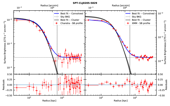
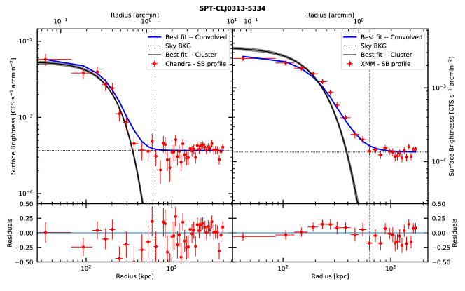
Figure 11: Chandra (left) and XMM-Newton (right) measured NXB subtracted surface brightness (red points). The best-fitting model is the Vikhlinin et al. (2006) functional (solid black line) form plus a constant sky background (horizontal dotted line); it is convolved with the intrumental PSF and it is shown with a blue line. In case of Chandra the PSF is simply a diagonal matrix with ones on the diagonal, while for XMM-Newton it is calculated as in Sect. 2.2.2. In the bottom panels we show the residuals ($\frac{\mu_{i}-N_{c,i}}{N_{c,i}}$). The dashed vertical line represents the location of $R_{500}$, as measured by solving HE equation (Equation 9) using the “forward T” method (see Sect. 3.1).

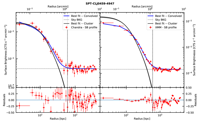
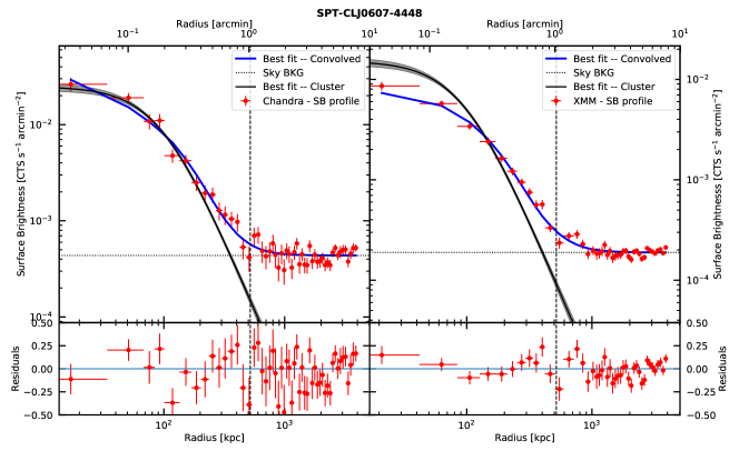
Figure 11: Continued

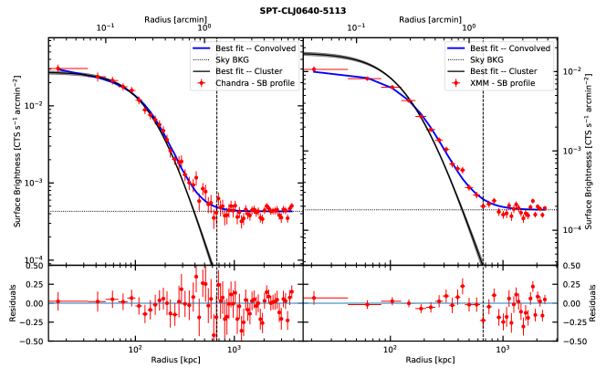
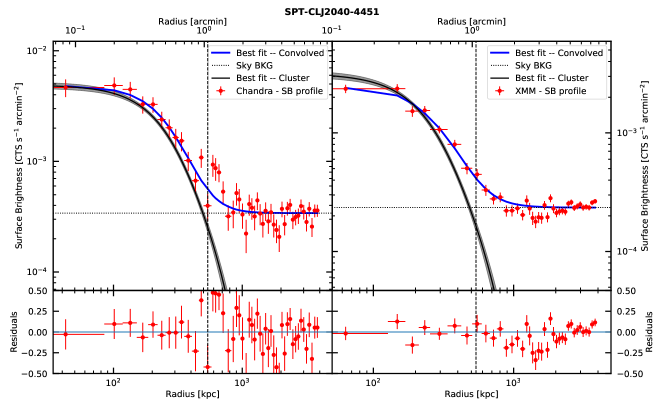
Figure 11: Continued

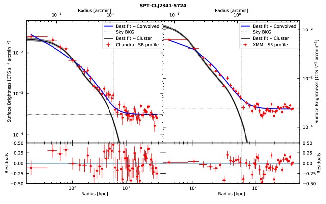
Figure 11: Continued

The surface brightness profiles and best-fit models are shown in Figure 11, while the best-fit parameters of the ICM model are given in Table 2. We note that the emissivity measurements of Chandra and XMM-Newton observatories are consistent with each other within 3%, therefore, calibration differences are irrelevant in the measurements of emissivity and number density (as also shown in Bartalucci et al., 2017b).

2.3 XMM-Newton Spectral Analysis

We extract spectra using the XMM-ESAS tools mos-spectra and pn-spectra (Snowden et al., 2008). Redistribution matrices (RMFs) and ancillary response files (ARFs) are created with rmfgen and arfgen, respectively. The point sources (see Section 2.2.1 for details) are excluded from the spectral analysis. The spectral fitting package Xspec v12.10 (Arnaud, 1996) with ATOMDB v3.0.9 is used in the analysis (Foster et al., 2012). The Galactic Column density is allowed to vary within 15% of the measured LAB value in our fits (Kalberla et al., 2005). The extended C-statistics are used as an estimator of the goodness-of-fit (Cash, 1979). The abundances are normalized to the Asplund et al. (2009) solar abundance measurements with the mean molecular weight $\mu=0.5994$ and the mean molecular mass per electron $\mu_{e}=1.1548$, and the ratio between number density of protons to electrons equal to $n_{p}/n_{e}=0.8527$. The MOS spectra are fitted in the energy band of 0.5–12 keV, while we use the 0.5–14 keV energy band for pn. We ignore the energy ranges between 1.2–1.9 keV for MOS, and 1.2–1.7 keV and 7.0–9.2 keV for pn due to the presence of bright and time-variable fluorescence lines. The energy band below 0.5 keV, where the EPIC calibration is uncertain, is eliminated from spectral fits. The source spectrum is modeled with an absorbed single-temperature thermal model apec with varying temperature, metallicity, and normalization. For the clusters with multiple observations the model parameters are tied between multiple spectra and fitted jointly.

The particle background is determined using the rescaled filter-wheel-closed spectra, that allows us to measure the intensity and the spectral shape. On top of this, we include an additional model component for the residual soft protons (Salvetti et al., 2017), modeled as a broken power law with shape fixed (slopes 0.4 and 0.8 and break energy 5 keV Leccardi & Molendi, 2008) and normalization free. Regarding the sky background, we model it as the sum of three components: (i) the cosmic X-ray background (CXB) with an absorbed power law with photon index fixed to 1.46, (ii) the galactic halo (GH) with an absorbed APEC model with temperature free to vary in the range [0.1-0.6] keV, and (iii) the local bubble (LB) with an APEC model with temperature fixed to 0.11 keV(Snowden et al., 2008; Leccardi & Molendi, 2008). The normalizations of the CXB, LB, and GH background components are set free. To find the sky parameters we fit the background region, by extracting a spectrum 5 arcmin ( $\sim 5R_{500}$ ) away from the core. We impose gaussian priors on these parameters with width equal to the parameter uncertainty found in the fitting of the background region.

We first extract the XMM-Newton spectra within $R_{500}$ to measure the redshifts of the clusters from the X-ray data. Fitting the spectra within $R_{500}$, so that the statistics are of high quality to determine an accurate X-ray redshift. We fit these spectra using an absorbed single temperature thermal model with free temperature, metallicity, redshift, and normalization. Taking into account the gain calibration uncertainty of XMM-Newton pn at 3 keV (the redshifted position of the Fe-K line) of 12 eV (private communication with the XMM-Newton calibration team), we find that the redshifts are consistent with the previously reported photometric (Bleem et al., 2015) and spectroscopic redshifts (Bayliss et al., 2014; Khullar et al., 2019; Stalder et al., 2013) within $2\sigma$ confidence level for these clusters. A comparison of redshifts based on X-ray data with photometric and spectroscopic redshifts are shown in Figure 2. We point out that for SPT-CLJ0459-4947 the previously reported redshift (Bocquet et al., 2019) is measured using the position of the Fe-K line from XMM-Newton data from LP by A. Mantz.

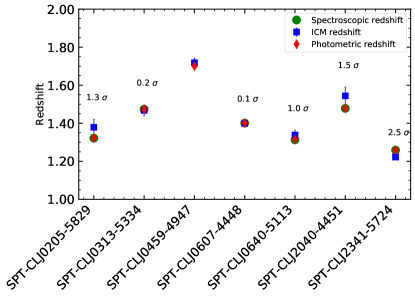
Figure 2: Comparisons of X-ray redshifts (in blue) with the photometric redshifts in red (Bleem et al., 2015), spectroscopic redshifts in green Bayliss et al. (2014); Stalder et al. (2013); Khullar et al. (2019). The error bars indicate the sum of statistical and systematic uncertainties at 1$\sigma$ level.

To examine the radial profiles of thermodynamic properties, we next extract the spectra from concentric annuli with sizes increasing logarithmically around the cluster centroid. The minimum width of annuli is set to be $\sim$15 arcsec to minimize the effect of the XMM-Newton’s PSF, but still having a large enough statistic to determine the projected temperature. We group the output spectra to ensure having a minimum of 5 counts per bin. The XMM-Newton PSF is taken into account using the cross-talk ARFs generated by the SAS task arfgen. This method allows the spectra to be co-fitted by taking into account the cross-talk contribution to an annulus from another region (Snowden et al., 2008; Ettori et al., 2010). The use of flat constant priors on the temperature, metallicity, and the use of the ‘jeffreys’ prior on the normalizations (i.e. ${\rm Prior(K_{apec)}}={\rm K_{apec}^{-1}}$) allows us to account for the uncertainty on the sky background as well as the uncertainty in their free parameters. The spectra are fit using the Monte Carlo Markov Chain (MCMC) implementation in Xspec of the Goodman-Weare algorithm (Goodman & Weare, 2010), with 50000 steps and 1000 burn-in period to ensure we investigate the parameter space and derive the uncertainties on free parameters (temperature, metallicity, and normalization) in our fitting software. At the end of this process, we obtain the best-fit projected temperatures and their covariance matrix, which are easily computed using the MCMC chain.

To obtain the three-dimensional deprojected temperature profile of each cluster, we project the ICM temperature model on the plane of the sky by taking into account emission weighting to determine spectroscopic-like temperature (Mazzotta et al., 2004),

$$T_{\rm 2D,sl,i}=\frac{\int n_{e}^{2}T_{\rm 3D}^{1-\alpha}dV}{\int n_{e}^{2}T_{\rm 3D}^{-\alpha}dV}.$$ (6)

where $\alpha=3/2$ and $n_{e}$ is the electron number density, $T_{sl}$ is the predicted 2D spectral temperature, and the temperature model $T_{3D}$ is a widely used phenomenological model to describe the temperature profiles (Vikhlinin et al., 2006):

The 3D ICM model we used in this work is

$$T_{3D}(r)=T_{0}\frac{\frac{T_{min}}{T_{0}}+\left(\frac{x}{r_{cool}}\right)^{a_{cool}}}{1+\left(\frac{x}{r_{cool}}\right)^{a_{cool}}}\frac{1}{\left(1+\left(\frac{x}{r_{t}}\right)^{2}\right)^{\frac{c}{2}}}$$ (7)

We first minimize the $\chi^{2}=-2\log\mathcal{L}$ using the Nelder-Mead method (Gao & Han, 2012). Then we fit using the Markov Chain Monte Carlo method using the code emcee (Foreman-Mackey et al., 2013) using gaussian priors centered around the Nelder–Mead method results and with a sigma of 0.5 (or 1.15 dex). We use 10000 steps with burn-in length of 5000 steps to have resulting chains independent of the starting position and thinning of 10 to reduce the correlation between consecutive steps. The likelihood adopted in the fit is;

$$\log\mathcal{L}=-\left(\log T_{obs}-\log T_{sl}\right)\Sigma_{i,j}\left(\log T_{obs}-\log T_{sl}\right)^{\rm\mathbf{T}}$$ (8)

where $T_{obs}$ and $T_{sl}$ are the arrays of the measured spectral temperatures and of the spectroscopic-like projected temperatures as of Equation (6) respectively, and $\Sigma_{i,j}$ is the spectral log-temperature covariance matrix, see Sect. 2.3. Thus a $\chi^{2}$-like log-likelihood, where the temperature distribution in each annulus is assumed to be a log-normal (Andreon, 2012) and the full covariance between the annuli is considered. The best-fit parameters for the temperature profile are given in Table 3.

3 Results

In this section we explore thermodynamic properties (e.g., density, temperature, pressure, and entropy) of the high redshift SPT clusters in our sample taking advantage of the SPT SZ survey’s clean selection function and its high sensitivity. We further compare the thermodynamic properties of the ICM of the clusters in our sample with the X-COP sample to investigate their evolution with redshift. The X-COP sample is selected based on the Planck signal-to-noise ratio including only low redshift clusters with $z<0.1$ (Ghirardini et al., 2018b, G18 hereafter). In G18, the authors were able to recover ICM properties out to the Virial radius using the joint X-ray and SZ analysis, adding on to the previous studies which probe the region within $R_{500}$ by joining X-ray and SZ observations (e.g. Ameglio et al., 2007; Hasler et al., 2012; Bonamente et al., 2012; Eckert et al., 2013b, a; Shitanishi et al., 2018). We further remark that the analysis done for the high redshift clusters is almost identical to the analysis applied in G18 for the X-COP cluster sample, allowing us for controlled measurement of the evolution in the thermodynamic quantities.

The self-similar model (Kaiser, 1986), which assumes purely gravitational collapse, predicts a particular evolution with redshift of the cluster properties once they are scaled based on their common quantities, e.g. mass within an overdensity radius (Voit et al., 2005). We, therefore, measure the mass of our clusters and rescale our thermodynamic quantities with this mass within $R_{500}$. In the next section we describe our method for the mass reconstruction under the assumption of hydrostatic equilibrium (HE), and then show the thermodynamic profiles and describe their properties.

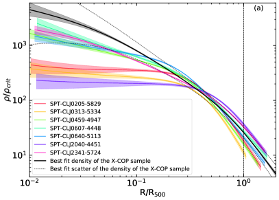
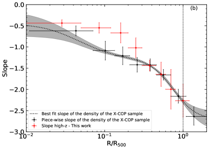
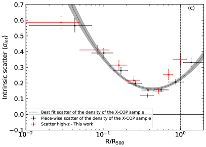
Figure 3: Top Panel: (a) Density profiles from the sample. The solid black line represents the average density profile of the X-COP clusters. (b) Slope of the density profile of the high-z SPT-selected clusters obtained by the piece-wise power-law fitting technique is shown with red crosses compared to those of the X-COP clusters (shown in the dotted black line and the black crosses). Bottom Panel: (c) Scatter in the density profiles of the high-z SPT-selected clusters (red crosses) and the X-COP clusters (black crosses). The vertical dashed line represents the location of $R_{500}$ in all panels.

3.1 Total Cluster Mass Reconstruction

A common way to measure the total mass $M_{500}$ is to use mass proxies calibrated with an X-ray or SZ observable, e.g., $L-M$ or $\xi-M$ scaling relations (e.g. Pratt et al., 2009; Bocquet et al., 2019; Bulbul et al., 2019). However, to avoid introducing a bias in our results by using the evolution in a specific scaling relation, we directly measure the cluster total mass using X-ray observations. The direct measurements based on X-ray data can be obtained from the thermodynamic properties using the assumption of hydrostatic equilibrium and spherical symmetry, i.e.

$$M(<R)=-\frac{R\,k_{B}\,T}{G\,\mu m_{p}}\left[\frac{d\log\rho_{g}}{d\log R}+\frac{d\log T}{d\log R}\right].$$ (9)

where $G$ gravitational constant, $m_{p}$ mass of the proton, and $\rho_{g}$ is the gas density. There are several methods that are used in the literature to solve the previous equation (see Ettori et al., 2013, for a review). Throughout this work, we adopt a “forward” modeling approach to obtain a measurement of $M_{500}$, the total cluster mass within $R_{500}$. We make use of the best-fitting density and temperature profiles as recovered in Sect. 2.2 and 2.3 respectively, propagating them through the HE equation to recover the mass profile.

This method has the advantage of starting from smooth thermodynamic profiles, where the large number of parameters in these functional forms allow us to reproduce the density and temperature profiles over a large radial range. We direct the reader to the Appendix A for comparison with literature results, and with other mass reconstruction techniques we have employed to solve Equation (9).

3.2 Density, Temperature, Pressure, and Entropy Profiles

The deprojected electron density profile $n_{e}(r)$ (see Sect. 2.2.4) obtained from surface brightness analysis is first converted into gas density $\rho(r)=\mu_{e}m_{p}n_{e}(r)$ and then rescaled by the critical density of the Universe $\rho_{c}=\frac{3H^{2}(z)}{8\pi G}$, where $H(z)=H_{0}E(z)$ and $E^{2}(z)=\Omega_{\Lambda}+\Omega_{m}(1+z)^{3}$. Panel (a) of Figure 3 shows the gas density profiles of the sample. We notice that, in the outskirts, the profiles of the SPT-selected high-z and the Planck selected nearby X-COP clusters are fully consistent with each other, while in the core the SPT-selected high-z profiles are factor of a few smaller. In the core, the observed scatter (measured as in Eq. 6 in G18) is an order of magnitude both in the SPT-selected high-z and the Planck selected nearby X-COP clusters, due to the cool core/non-cool core states in both samples, i.e. the effect of this dichotomy mostly dominates the scatter near the core. The scatter becomes minimal around 0.4 $R_{500}$, at the same location where X-COP clusters reach their minima in the scatter. Towards $R_{500}$ in the outskirts the scatter increases again in both samples. The increase in the high redshift sample is faster, reaching the value of about 0.35 at $R_{500}$, while the scatter in the X-COP sample remains at 0.2 at the same radius. A comparison of the scatter is seen in panel (c) of Figure 3.

To be able to measure the slope of the density profiles, we perform a piece-wise power-law fitting technique as described in detail in G18. Comparing our sample with the nearby X-COP clusters, we find that in the core, the slope in our sample is flatter compared to the X-COP clusters, while in the outskirts ($>0.3R_{500}$) the mean slopes are consistent with each other (see panel (b) of Figure 3).

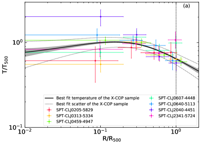
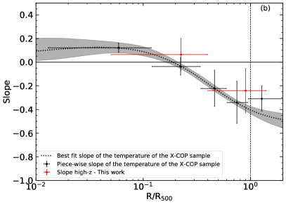
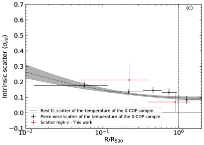
Figure 4: Same as Figure 3, but for the temperature profiles.

Next, we study the temperature profiles of the SPT clusters and compare them with the nearby X-COP clusters. For this comparison, the spectroscopic temperature profiles (see Sect. 2.3 for details) are scaled by the self-similar $T_{500}$, also used in Equation 10 of G18 for the X-COP clusters (Voit et al., 2005):

$$T_{500}=8.85\text{\ keV}\left(\frac{M_{500}}{h_{70}^{-1}10^{15}M_{\odot}}\right)^{2/3}E(z)^{2/3}\left(\frac{\mu}{0.6}\right)$$ (10)

where the total mass M₅₀₀ is measured in Sect. 3.1, and used self-consistently in calculations of R₅₀₀ and $T_{500}$. In panel (a) of Figure 4, we compare the rescaled temperature profiles of the SPT high-z clusters with the nearby X-COP clusters. We find that the scaled temperature profiles in the two samples are consistent with each other in the entire radial range out to $R_{500}$. The size of the PSF of XMM-Newton is comparable to the size of the core of these high-redshift clusters, therefore we cannot resolve well temperatures within $<$150 kpc, or 0.1 $R_{500}$. Performing a piece-wise power-law analysis in two radial bins, we obtain similar slopes and the intrinsic scatter in the temperature profiles when comparing them with the X-COP clusters results.

The pressure profiles are obtained by combining the deprojected density and temperature profiles as $P=n_{e}T_{e}$. Pressure profiles can be constrained from both X-ray and SZ observations and used for constraining astrophysical properties and the total mass of clusters out to their Virial radius (Bonamente et al., 2012; Ghirardini et al., 2018a).

We rescaled the pressure using the self-similar pressure $P_{500}$ as described in Nagai et al. (2007):

$$P_{500}=3.426\times 10^{-3}\text{\ keV}\text{\ cm}^{-3}\left(\frac{M_{500}}{h_{70}^{-1}10^{15}M_{\odot}}\right)^{2/3}E(z)^{8/3}\cdot\\ \cdot\left(\frac{f_{b}}{0.16}\right)\left(\frac{\mu}{0.6}\right)\left(\frac{\mu_{e}}{1.14}\right)$$ (11)

Panel (a) of Figure 5 shows a comparison of the rescaled pressure profiles of our sample of high-z clusters with the X-COP sample. We find that in the core of SPT high-z clusters the rescaled pressure is on average lower and flatter compared with what is measured in nearby clusters. In the outskirts, pressure becomes consistent with the finding of low redshift X-COP clusters. The scatter is also fully consistent between high and low redshift clusters in all our radial points except the outermost at $R_{500}$, when at high redshift it is 20% higher.

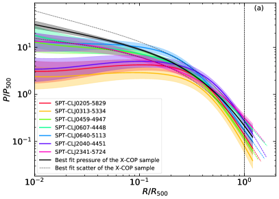
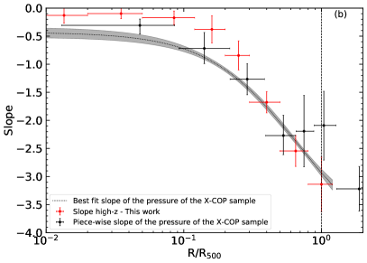
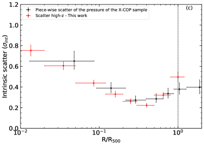
Figure 5: Same as Figure 3, but for the pressure profiles.

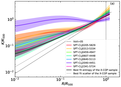
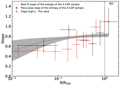
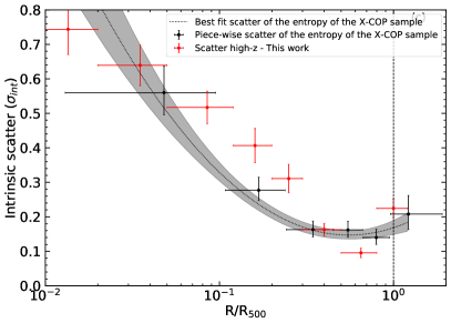
Figure 6: Same as Figure 3, but for the entropy profiles.

Another thermodynamic property that could be extracted from X-ray observations is the entropy. Entropy is often used to constrain the clumpiness and self-similarity in cluster outskirts (Walker et al., 2012; Urban et al., 2011; Bulbul et al., 2016). The entropy profiles are obtained using the relation, $K=Tn_{e}^{-2/3}$. Similarly, the entropy is rescaled with the self-similar value $K_{500}$ for comparison (see Voit et al., 2005):

$$K_{500}=1667\text{\ keV cm}^{2}\left(\frac{M_{500}}{h_{70}^{-1}10^{15}M_{\odot}}\right)^{2/3}E(z)^{-2/3}\cdot\\ \cdot\left(\frac{f_{b}}{0.16}\right)^{-2/3}\left(\frac{\mu}{0.6}\right)\left(\frac{\mu_{e}}{1.14}\right)^{2/3}$$ (12)

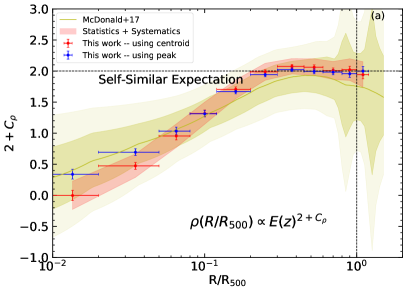
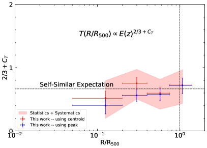
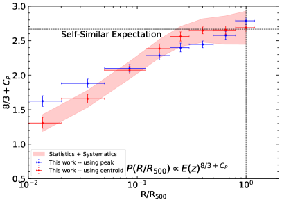
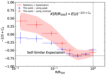
Figure 7: Top Panel: (a) Evolution in the density profiles as a function of redshift obtained using the centroid (in red) and X-ray peak (in blue). The red shaded region around our data points represents the sum in quadrature of the statistical and systematic uncertainties (see Sect. 4 for details). The yellow shaded area represents the same result as found by MD17. Zero values of $2+C_{\rho}$ indicate no evolution with redshift. The self-similar evolution of $C_{\rho}=0$ (corresponding to $\rho\propto E(z)^{2}$) is represented by an horizontal dashed line. The other panels are the same but for temperature (b) with self-similar predicted evolution corresponding to $T\propto E(z)^{\frac{2}{3}}$, for pressure (c) with self-similar predicted evolution corresponding to $P\propto E(z)^{\frac{2}{3}}$, and entropy (d) with self-similar predicted evolution corresponding to $K\propto E(z)^{-\frac{2}{3}}$. Moreover for pressure and entropy, below 0.1 $R_{500}$ the values of the evolution are extrapolated because temperature measurements are not resolved on smaller scales. The vertical dashed line represents the location of $R_{500}$ in all panels.

In Figure 6 we show the entropy profiles of the sample, the slope of the entropy, and the intrinsic scatter. An excess is observed in the entropy compared to self-similarity within (0.3$R_{500}$) near the core. We attribute this excess to non-gravitational processes (e.g., AGN feedback, infalling substructures, merging activities) in the cores. A similar entropy excess in the core was reported in nearby low redshift clusters (Urban et al., 2014; Bulbul et al., 2016; Ghirardini et al., 2018b; Walker et al., 2019), however smaller than the entropy excess observed in these high-z clusters. The high-z entropy excess may be due to the increased incidence of non-gravitational effects, e.g. galaxy and cluster formation, minor mergers at higher redshifts that triggers AGN activity (Bîrzan et al., 2017; Hlavacek-Larrondo et al., 2012; McDonald et al., 2016).

The entropy profiles are flat in the cores, steepen and become consistent with the self-similar model beyond $\sim$ 0.2$R_{500}$, similarly and fully consistent with the entropy profiles in the outskirts of nearby clusters (see Walker et al., 2019, for a review and references therein). The intrinsic scatter is comparable for both samples.

3.3 Evolution of thermodynamic Properties with Redshift

In this section, we investigate the redshift evolution of thermodynamic properties of the ICM and measure the deviation from self-similarity of our sample. Following a similar approach described in MD17, we determine the evolution of the density in different radial bins. We characterize the evolution of the thermodynamic quantities using the functions given below

$$\begin{cases}\left(\rho\right)_{z}=\left(\rho\right)_{z=0}\cdot E(z)^{2+C_{\rho}}\\ \left(T\right)_{z}=\left(T\right)_{z=0}\cdot E(z)^{2/3+C_{T}}\\ \left(P\right)_{z}=\left(P\right)_{z=0}\cdot E(z)^{8/3+C_{P}}\\ \left(K\right)_{z}=\left(K\right)_{z=0}\cdot E(z)^{-2/3+C_{K}}\\ \end{cases}$$ (13)

where $C_{\rho,T,P,K}$ represent the deviation with respect to self-similar values for the evolution (Kaiser, 1986) of density, temperature, pressure, and entropy. Starting from the density, temperature, pressure, and entropy profiles of the nearby X-COP sample, we infer the expected profiles at the redshifts of the SPT high-z sample assuming a simple deviation from the self-similar evolution, as indicated in Equation (13). We, then, compare these profiles with the thermodynamic profiles of the SPT clusters using a log-likelihood $\log\mathcal{L}=-\chi^{2}/2$ to fit and to determine the best-fit evolution parameters $C_{\rho,T,P,K}$. The best-fit parameters of these fits are given in Table 6. The uncertainties of the X-COP profiles as well as their measured scatter, and the uncertainties on $R_{500}$ and $Q_{500}$, see Eq. (10), (11), and (12), are propagated through the fit. We also include the systematic uncertainties related to our observations in our measurements (see Section 4 for details). The systematic and statistical uncertainties are summed in quadrature to estimate the total uncertainty.

We note that the cluster centers are determined from the Chandra data and initial results are obtained using the centroid of the large scale ICM emission in this analysis. The choice of cluster center plays an important role especially when measuring the evolution of the central cluster properties (Sanders et al., 2018). To investigate the effect of the center location, we determine the evolution in density using both the centroid and the X-ray peak. The evolution in density, temperature, pressure, and entropy profiles obtained using both the centroids (red) and X-ray peaks (green) are shown in Figure 7.

We find no evolution in the density at small radii ($\sim 0.3R_{500}$) using large scale centroids. The self-similar evolution in cluster cores is excluded significantly by $\sim$11$\sigma$. Using of the X-ray peaks instead of the centroids, the evolution values move slightly towards self-similarity in the core. However, the departure from self-similarity is still significant at a $\sim$9$\sigma$ confidence level. We also note that the intrinsic scatter in density of high redshift clusters, shown in Figure 3 panel (c), at small radii, is similar to that of the low X-COP redshift clusters. Non-gravitational phenomena, e.g., Active Galactic Nuclei feedback, sloshing, dominate the physical processes in cluster cores and can affect the evolution in the core of the clusters. Thus, our finding may point that non gravitational physical processes that regulate cluster cores were already in place since a redshift of 1.8 (with look back time of $\sim$10 Gyr). Our results in cluster cores are consistent with the results in MD17 at the 1$\sigma$ confidence level. However the uncertainties in the measurements are reduced at least by a factor of two. Sanders et al. (2018) suggests that use of the X-ray peak instead of centroids could mimic a potential evolution in cluster cores and bias the results in evolution studies. Changing the cluster center does not significantly affect our results.

At large radii, the evolution in density becomes consistent with the self-similar expectation around 0.1$R_{500}$ and remains fully consistent out to $R_{500}$. MD17 also reported the best-fit evolution consistent with the self-similarity, however due to the limited statistics the authors could not rule out no evolution scenario. We tightly constrain self-similarity in cluster outskirts and confirm it with a higher significant level. We also observe an increase of the scatter on cluster density profiles (see Figure 3) in cluster outskirts. This may imply that although the cluster-to-cluster variance in the outskirts increases because of larger mass accretion rates and merger activity at higher redshifts (Wechsler et al., 2002; Fakhouri & Ma, 2009; Tillson et al., 2011; Avestruz et al., 2016), the average evolution in density, however, remains consistent with this self-similarity.

In the case of temperature profiles, we don’t measure any significant deviation from self-similarity from the cluster cores out to $R_{500}$. The intrinsic scatter is also consistent with that of the low redshift clusters within uncertainties (see Figure 4). Therefore, the cluster temperature evolution and the cluster to cluster variance do not seem to change from low to high redshifts. The change of the cluster centre makes a very small difference and does not change the results. This is not surprising considering the large uncertainties on temperature measurements.

We observe a mild evolution in pressure profiles in cluster cores. Similarly, the evolution becomes consistent with self-similarity at $\sim$0.1 $R_{500}$ and larger scales. At small scales, pressure profiles deviate significantly from self-similar evolution at a 9$\sigma$ level. Using the X-ray peak as the cluster center does not change the results significantly.

Interestingly, in the core, a mildly significant ($\sim 3\sigma$ confidence) evolution is observed for the entropy, if we use the centroid as the cluster center. Changing the cluster center to the X-ray peak reduces significantly the observed evolution. In the outskirts the evolution becomes fully consistent with self-similarity, regardless of the center used.

It’s important to remind the reader that the evolution measured in cluster cores for pressure and entropy is quite dependent upon the adopted cluster temperature model, because the first temperature bin is very large, encapsulating the entire cluster core, $<0.1R_{500}$.

3.4 Polytropic index

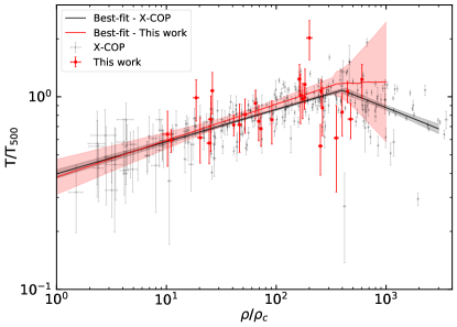
Figure 8: Rescaled temperature against rescaled density in high redshift cluster sample (in red) and in low redshift clusters (in black, Ghirardini et al., 2019). The lines represent the best-fit broken power-law to the data. In particular, we find that the slope in the relation is consistent in low and high redshift clusters in the low density regime, i.e. in cluster outskirts, supporting again the self-similar model of cluster evolution.

The global structure of the ICM can be effectively described by a polytropic equation of state $P_{e}=K\rho^{\Gamma}$, where the polytropic index is indicative of stratification of the ICM (Shaw et al., 2010). Both simulations (Komatsu & Seljak, 2001; Ostriker et al., 2005; Ascasibar et al., 2006; Capelo et al., 2012) and observations (Markevitch et al., 1998; Sanderson et al., 2003; Bulbul et al., 2010; Eckert et al., 2015; Ghirardini et al., 2019) find that the stratific ation of the ICM, especially in the outer part, is well represented by a polytropic equation of state with $\Gamma$ in the range 1.1-1.3. In particular, the X-COP collaboration reports that the value of $\Gamma$ in cluster outskirts, where $\rho/\rho_{c}\lesssim 400$, is $\Gamma=1.17\pm 0.01$ at redshifts below 0.1. However, the polytropic index in the high redshift Universe, or its evolution, has never been investigated. We find that the polytropic index, see also Figure 8, is $1.19\pm 0.05$ in low density regions, i.e. in the cluster outskirts. This value is fully consistent with the value measured at low redshifts in the X-COP clusters, indicating that there is no significant evolution with redshift, i.e. the ICM stratification is the same at low and high redshift. In high density regions, i.e. in the core, we are not able to resolve the index due to the large size of the XMM-Newton PSF.

4 Systematics

Thermodynamic	HE		Clumping	Progenitor		Calibration
At	0.01 $R_{500}$	$R_{500}$	-	0.01 $R_{500}$	$R_{500}$	0.01 $R_{500}$	$R_{500}$
Density	0.02	0.10	0.058	0.14	0	0.03	0.09
Temperature	0.08	0.10	0.061	0.12	0	0.07	0.04
Pressure	0.09	0.19	0.061	-		0.04	0.13
Entropy	0.10	0.11	0.025	0.25	0	0.03	0.01

Table 4: Range in which each systematic bias discussed in Sect. 4 affects each thermodynamic quantity in the core and at $R_{500}$. The thermodynamic biases are, from left to right: 1) hydrostatic bias caused by how the profiles are rescaled, 2) clumping bias caused by the presence of unresolved clumps, 3) bias caused by the fact that SPT high-z clusters are not exactly the progenitors of the redshift 0 clusters we are comparing them with, and 4) calibration bias caused by difference between Chandra and XMM-Newtontemperatures.

In this section, we examine several systematic uncertainties that affect our results on the evolution of the thermodynamic properties of clusters, evaluating their magnitudes. The variation of the thermodynamic property $\mathrm{Q}$ can be converted into the systematic uncertainty on the evolution following the formula below.

$$\mathrm{Q}+\Delta\mathrm{Q}=E(\hat{z})^{k}\cdot\mathrm{Q}$$ (14)

where $\hat{z}$ is the average redshift of our sample, and $k$ is the systematic uncertainty on the evolution of each thermodynamic property Q. Solving this equation for the systematic uncertainty $k$ gives the following equation:

$$k=\frac{\log\left(1+\frac{\Delta\mathrm{Q}}{\mathrm{Q}}\right)}{E(\hat{z})}.$$ (15)

We consider the systematic uncertainties related to hydrostatic mass bias, clumping factor, cluster progenitors, and calibration differences between XMM-Newton and Chandra below. In Table 4 we show the amplitude of the mass bias on each thermodynamic quantity in the core and at $R_{500}$.

4.1 Mass bias

The evolution measured on a thermodynamic property is affected by a potential bias due to the assumption of hydrostatic equilibrium. If the hydrostatic masses we use in this work are biased by a factor of $(1+b)$, this bias translates to a bias in the fiducial radius that can be written as;

$$\left(\frac{R}{R_{500}}\right)_{z}=\left(\frac{R}{R_{500}}\right)_{z=0}\times(1+b)^{-\frac{1}{3}}.$$ (16)

And also it translates into an uncertainty on a rescaled thermodynamic property Q as;

$$\left(\frac{\mathrm{Q}}{\mathrm{Q_{500}}}\right)_{z}=\left(\frac{\mathrm{Q}}{\mathrm{Q}_{500}}\right)_{z=0}\times(1+b)^{-\frac{2}{3}}$$ (17)

where $Q=T,P,K$

A bias, which is introduced by mass, can mimic evolution on these thermodynamic properties. Unfortunately, evolution measurements and mass bias are highly degenerate, thus it is not possible to fit Equation (13) and Equation (16)-(17) simultaneously to constrain the mass bias and the evolution with redshift. Given that the low redshift X-COP sample and high redshift SPT sample have very similar selection criteria, i.e. a selection based on SZ S/N, and the masses are obtained in a similar way, i.e. assuming HE, the mass bias is expected to affect the results from the two samples by the same amplitude and direction.

An estimate of the mass bias can be obtained by measuring the average ratio between several mass measurements. In Sect. 3.1 we have described our reference method of solving the HE equation to measure $M_{500}$, and, in Appendix A, we compare this measure with other techniques, and other masses in the literature obtained from scaling relations. Figure 9 shows the cluster masses obtained through these methods. To estimate this bias we measure the average ratio between the measured masses and the mass obtained using the method described in Sect. 3.1. Since the error bars are not homogeneous, we apply a bootstrap method through all the mass measurements for each cluster. In practice, we measure the mass bias $10^{6}$ times where each time a new distribution of masses is drawn from the masses shown in Figure 9. This method yields a mass bias of $1+b=1.12\pm 0.01$. The result implies that high redshift clusters have 12% higher mass bias compared to the nearby clusters. Given that clusters at high redshifts are still forming and not yet thermalized, an increase in the non-thermal pressure support due to gas motions in their outskirts and elevated AGN activity in their cores resulting in an increase in mass bias with redshift is expected.

Using the mass bias obtained above, we then estimate the corresponding systematic bias in the evolution. This bias affects both x and y axes, except for density where the rescaling on the y-axis is independent of mass. The bias is translated into

$$\Delta Q=\Delta R\cdot\frac{dQ}{dR}=(\Delta M)^{1/3}\cdot\frac{dQ}{dR}$$ (18)

on the x-axis, and

$$\Delta Q=(\Delta M)^{2/3}$$ (19)

on the y-axis, then by summing up in quadrature these two values and applying Equation (14) and Equation (15) we measure the systematic uncertainty on the evolution of the thermodynamic quantities caused by the mass bias.

4.2 Clumping factor

Unresolved clumps in our observations can lead to higher local densities measured and can bias the observed thermodynamic quantities. In G18 the authors correct the density for the presence of these clumps by both removing the extended sources contaminating the FoV, and by also computing the median of surface brightness distribution in each annulus, which has been shown to be unbiased by the presence of high density unresolved substructures (Zhuravleva et al., 2013; Roncarelli et al., 2013). In particular, to compute the median, a Voronoi tessellation algorithm needs to be performed (Diehl & Statler, 2006) to produce cells containing surface brightness elements. In this work, we eliminate the detected point and extended sources from our analysis. Due to low counts observed and the small extension of the clusters on the sky, the cells produced via the Voronoi tessellation algorithm would be very few and highly correlated with each other. Therefore, it’s not possible to compute the median of the surface brightness distribution in the same way as applied to the X-COP sample. Instead, we estimate this bias by adopting the upper limit of 10% within $R_{500}$ measured in a sample of ROSAT clusters in Eckert et al. (2015). We find that the density profiles are biased by a systematic uncertainty of $\Delta\rho/\rho=0.10$. This translates into a systematic on the density measurements of $\sim$0.06 (see Equation 15).

For the other thermodynamic properties, we combine the effect aforementioned with the bias of 5% in the pressure arising by the presence of clumps (as measured in simulations by Khedekar et al., 2013, where the 5% refers to the upper limit within $R_{500}$). This translates into a bias of 5% on the temperature, consistent with the predicted theoretical bias by Avestruz et al. (2016), and -2% bias on the entropy.

4.3 Progenitors

It is possible that these SPT-selected high redshift clusters are not the progenitors of the low redshift clusters in X-COP. In fact, the predicted mass of the SPT clusters is expected to be greater than $10^{15}M_{\odot}$ at redshift zero when the mass growth curve is taken into account (Fakhouri et al., 2010). Therefore, the SPT-selected clusters are more massive than the X-COP clusters (Ettori et al., 2018), where the reported masses are less than $10^{15}M_{\odot}$. We treat the effect due to the fact that the X-COP clusters could be evolved from a different population of clusters than the SPT clusters as a systematic uncertainty.

To estimate this bias we assume that the gas density follows the dark matter density as a first approximation. We then use a concentration-mass-redshift relation in Amodeo et al. (2016) to calculate the relative change in the density from a cluster with mass of $15\cdot 10^{14}M_{\odot}$, i.e. the expected mass of SPT clusters at redshift of 0 Fakhouri et al. (2010), to a mass of $7\cdot 10^{14}M_{\odot}$, i.e. the average mass of X-COP clusters. Assuming that pressure follows the Universal pressure profile, we estimate the thermodynamic quantities. These values are then propagated as systematic errors as shown in Equation (15). The results in the core and in the outskirts are given in Table 4. We note that the self-similar model predicts an evolution which is independent of mass. Therefore, once the thermodynamic quantities are rescaled with their self-similar value, the fact that they are too massive to be the progenitors of the X-COP clusters is of minor importance, especially at large radii.

4.4 Calibration Difference between Chandra and XMM-Newton

Calibration differences between Chandra and XMM-Newton are described in the literature. Temperature measurements can be biased up to 40% depending on the energy band used and cluster temperature (e.g. Schellenberger et al., 2015, and references therein). On the other hand, density measurements by Chandra and XMM-Newton are fully consistent within the uncertainties (see Bartalucci et al., 2017a, and also Sect. 2.2.4).

To quantify the bias due to calibration differences, we extract both XMM-Newton and Chandra spectra of the region within $R_{500}$, and fit the spectra using a single temperature thermal apec model. We note that in the case of the SPT high redshift clusters, it is not possible to measure temperature profiles using Chandra observations in several radial bins due to the limited statistics. A comparison of measured single temperatures is shown in Figure 10. We find the temperature measurements are consistent with each other within statistical uncertainties. However, we note that the uncertainties on the Chandra measurements are large because of limited statistics.

To estimate the systematic uncertainty on each thermodynamic quantity $Q$ caused by this discrepancy in the temperature is not trivial. The increase of the temperature would lead to an increase in the total mass by the same amount, if the slope of temperature profile does not change. Schellenberger et al. (2015) report that temperature measurements based on Chandra data are, on average, 17% higher temperatures than those derived from XMM-Newton for the average mass of the clusters in our SPT sample. Thus, a systematic of 17% on the temperature becomes a 17% systematic on the mass, thus a 5.7% bias on $R_{500}$ (a third considering the propagation of uncertainty), and 11.3% bias on $Q_{500}$ (two thirds considering that all self-similar quantities depend on mass with power of 2/3). Thus the variation on each thermodynamic quantity is

$$\frac{\Delta Q/Q_{500}}{Q/Q_{500}}=\underbrace{17\%}_{\textrm{ on Q}}-\underbrace{11.3\%}_{\textrm{ on Q}_{500}}-\underbrace{5.7\%\cdot\frac{dQ}{dR}}_{\textrm{ on R}_{500}}.$$ (20)

We point out that, for the last two terms, the variation on the rescaled thermodynamic quantity from the radial and the $Q_{500}$ rescaling is in the opposite direction with respect to the systematic bias on the quantity $Q$. Thus by computing the slope at each radius we get the relative rescaled thermodynamic variation at each radii, and finally using Equation (15) we obtain the systematic bias affecting the evolution of each thermodynamic quantity as given Table 4.

5 Conclusions

In this paper we have studied the thermodynamic profiles for the 7 most massive clusters at redshift above 1.2 in the SPT-SZ survey. These clusters were observed by both Chandra and XMM-Newton for a total clean exposure time of about 2 Ms. We combine the data from these two telescopes to recover density, temperature, pressure, and entropy profiles and examine their evolution with redshift from cluster cores to outskirts. Furthermore, we measure the temperature profiles of a complete set of SPT-selected high redshift clusters for the first time allowing us to reconstruct the total cluster masses under the assumption of hydrostatic equilibrium. Our results include the systematic uncertainties that are extensively studied in Section 4.

Deep XMM-Newton observations of the SPT-selected clusters have sufficient statistics to determine the redshifts from the X-ray data alone. The Fe-K line at 6.7 keV (rest frame) is clearly detected in the spectrum of each cluster in the sample. The centroids of these emission lines are used to measure the redshifts. We show that the redshifts obtained from the X-ray data of the SPT high-z clusters are consistent with the previously reported redshifts obtained through optical photometry and spectroscopy (Bayliss et al., 2014; Bleem et al., 2015; Khullar et al., 2019).

Combination of Chandra’s high spatial resolution and XMM-Newton’s large FoV and effective area is the most powerful way to measure thermodynamic profiles of clusters at high redshifts, $z>1.2$ from their cores (0.01 $R_{500}$) to the outskirts ($R_{500}$). Accurate measurements of temperature profiles enable a few key measurements for these clusters, e.g. total mass, pressure, and entropy. We are able to measure their total mass though the hydrostatic equilibrium assumption with relatively small uncertainities (10 - 20 %) at these redshifts. The hydrostatic masses are generally in good agreement with reported masses in the literature obtained through SZ signal-to-noise and scaling relations (Bleem et al., 2015).

We further measure the density, temperature, pressure, and entropy profiles of the high-z SPT cluster sample and compare their distributions with the previously reported thermodynamic properties of the nearby X-COP clusters. The scatter of all the thermodynamic quantities are similar in low and high redshift clusters in small spatial scales near the cores. At large radii, the scatter increases more steeply in the sample of high redshift clusters. This may be due to an increased frequency of merger events and higher mass accretion rate at high redshifts (Wechsler et al., 2002; Fakhouri & Ma, 2009; Tillson et al., 2011).

The average profiles of density, temperature, pressure, and entropy of high-z clusters are self-similar and consistent with those of the X-COP clusters at large spatial scales near $R_{500}$. Temperature profiles of high redshift clusters are self-similar at all radii. We also report that the polytropic index (1.19 $\pm$ 0.05) is fully consistent with that measured at low redshift clusters indicating that there is no significant evolution with redshift. The high observed scatter in density, pressure, and entropy in cluster cores is due to cool-core/non-cool core dichotomy in these cluster samples. The scatter in the thermodynamic properties becomes minimal at $0.4R_{500}$ and increases towards $R_{500}$ in the SPT-selected high-z clusters. The increase in the merger frequency and mass accretion rate in high-z clusters may contribute to high scatter in cluster outskirts (Wechsler et al., 2002; Fakhouri & Ma, 2009; Tillson et al., 2011).

We are also able to constrain the evolution in density and temperatures profiles of the cluster. Measurements of the evolution in entropy, pressure profiles with redshift also becomes available owing to precise temperature constraints for the first time. We find that the evolution in thermodynamic profiles deviates significantly from the self-similar evolution in cluster cores, while in the outskirts, the profiles are on average are in agreement with the prediction from the self-similar model. We find no evidence for evolution in the density in cluster cores, confirming the results in MD17. We point out that the analysis performed in this paper, and the one in MD17 are different in how self-similarity has been probed. We have considered two high-S/N cluster samples at low and high redshift, while in MD17 the authors have considered $\sim$100 low-S/N clusters. Therefore it is striking that two different analysis on two different samples yield the same results on the evolution of cluster density profiles. We observe only mild evolution in pressure and entropy profiles in cluster cores. On the other hand, the evolution of temperature profiles is in agreement with self-similarity. Utilization of the X-ray peak instead of the centroid of the large scale emission does not significantly affect our results.

Planned and future X-ray telescopes with sufficiently small spatial resolution and large effective area, e.g. Athena, Lynx will provide sufficient statistics to precisely measure temperature and density profiles down to kpc scales in the cores of a large sample of clusters (Nandra et al., 2013; Gaskin et al., 2019). These measurements will allow us to probe in detail the role of AGN feedback in the first clusters formed and to shed light onto the accretion processes in cluster outskirts and the structure formation in the Universe.

Appendix A Mass reconstruction

In this Appendix we solve the hydrostatic equilibrium equation with other approaches besides the one used throughout this paper, see Sect. 3.1.

A.1 Forward Modeling Approach

In Sect. 3.1 we have used a “forward” modeling where a temperature model is combined with a density model to solve hydrostatic equilibrium equation and recover the mass profile. However it is possible to do the same using a pressure model in combination with the density model, because it would be equivalent of doing the same but using pressure divided by density as the temperature model. We use the five-parameters functional form (Nagai et al., 2007) to model the pressure, and then recover the three-dimensional temperature profile by dividing it by the density profile. Then, everything goes like in Sect. 3.1. We indicate this method “forward P” distinguishing it from the one used in Sect. 3.1, indicated as “forward T”

A.2 Backward Modeling Approach

A popular model used in the literature is the “backward” modeling, which assumes a dark matter distribution, e.g. the Navarro-Frenk-White (NFW) model (Navarro et al., 1997), and then the observed temperature profiles are fitted against their profiles as predicted by the combination of the mass model with the density profile. Only two parameters are required to fully characterize the NFW mass model, scale radius and concentration (see Ettori et al., 2010, for details).

$$M_{tot,NFW}=\frac{4}{3}\pi\rho_{c}(z)500\frac{r_{s}^{3}c_{500}^{3}}{\log(1+c_{500})-\frac{c_{500}}{1+c_{500}}}\left(\log(1+\frac{r}{r_{s}})-\frac{\frac{r}{r_{s}}}{1+\frac{r}{r_{s}}}\right)$$ (A1)

or using the equation $R_{500}=r_{s}c_{500}$

$$M_{tot,NFW}=\frac{4}{3}\pi\rho_{c}(z)500\frac{R_{500}^{3}}{\log(1+c_{500})-\frac{c_{500}}{1+c_{500}}}\left(\log(1+c_{500}\frac{r}{R_{500}})-\frac{c_{500}\frac{r}{R_{500}}}{1+c_{500}\frac{r}{R_{500}}}\right)$$ (A2)

Since the large binsize of the annuli caused by the large XMM-Newton PSF of about 15 arcsec that corresponds to a physical size of 150 kpc, the constraints on the concentration parameter are very weak, meaning that the concentration is almost unconstrained. Thus we apply this technique two times, once leaving concentration completely free, i.e. with flat priors, and once choosing a gaussian prior on the concentration parameter, centered on the concentration–mass relation provided by Diemer & Joyce (2018): $\log c_{500}=0.885-0.049\log(M_{500}/5\,10^{14}M_{\odot})$, and with an instrinsic scatter of $\sigma_{log_{10}(c_{500})}=0.1$ (from Neto et al., 2007) propagated throught our analysis.

The fit is done using the code emcee (Foreman-Mackey et al., 2013), starting from a standard maximum likelihood fit, $\chi^{2}$ minimization using the Nelder-Mead method (Gao & Han, 2012), using 10000 steps with burning length of 5000 steps to have resulting chains independent from the starting position, and thinning of 10 in order to reduce the correlation between consecutive steps.

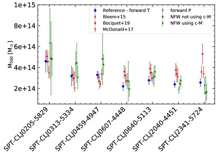
Figure 9: Mass comparison for the object in our sample. In red are the masses from the SPT catalog (Bleem et al., 2015), and the masses from SPT cosmological analysis (Bocquet et al., 2019). In black are the masses recovered by MD17 using the $M_{gas}-M_{tot}$ scaling relation. In green are the NFW best-fit masses in the two cases described in the text. In blue are the forward best-fit $M_{500}$ computed using functional form to fit the temperature and density profiles.

A.3 Reconstructed mass

Our reconstructed $M_{500}$, using the method described above and in Sect. 3.1, are shown in Figure 9. We compare our mass reconstruction among themselves, and with the SPT masses as calculated in the catalog (Bleem et al., 2015) using $M-\zeta$ fixed scaling relation, with the masses calculated from the scaling relations obtained for the SPT cosmological results (Bocquet et al., 2019), and with the masses used in MD17 which come from the $M_{gas}-M_{tot}$ scaling relations (Vikhlinin et al., 2009). Overall the masses we measure are consistent with all the other masses we are comparing with, with two peculiar cases: 1) SPT-CLJ0459-4947, for which the masses coming from the forward reconstruction agree with the other masses in the literature, i.e. the two SPT masses and the masses in MD17, but the NFW reconstruction prefers a higher mass. This can potentially indicate that the NFW mass model could not be the best model to describe the dark matter potential for this object. 2) SPT-CLJ2341-5724, which has all the masses coming from our analysis consistent within 1$\sigma$, however when comparing with the literature masses, we find that these are much higher than what we measure, indicating the possibility that this cluster does not fall on the scaling relations used to determine the literature masses. The recovered mass of SPT-CLJ0205-5829 has very large uncertainties. This is because the XMM-Newton 55 ks observation 0803050201 is highly flared, with only about 10 ks remaining after flare removal, and of top of that this cluster have a point source very close to the cluster center, thus decreasing the photon statistics with the resulting effect being larger error bars for the temperature, translating into large error bars on the mass since $M\sim T$.

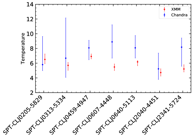
Figure 10: Comparison of a single temperature recovered from both Chandra and XMM-Newton from a circular region of width equal in radius to $R_{500}$

Cluster	$T_{\rm XMM}$	$T_{\rm CXO}$	$M_{\rm forward\ T}$	$M_{\rm forward\ P}$	$M_{\rm NFW,\ no\ c-M}$	$M_{\rm NFW,\ with\ c-M}$
	[keV]	[keV]	[$10^{14}M_{\odot}$]	[$10^{14}M_{\odot}$]	[$10^{14}M_{\odot}$]	[$10^{14}M_{\odot}$]
SPT-CLJ0205-5829	$6.51_{-0.57}^{+0.75}$	$5.81_{-0.82}^{+3.82}$	$4.59\pm 1.04$	$6.30\pm 3.31$	$4.88\pm 3.50$	$4.80\pm 1.58$
SPT-CLJ0313-5334	$5.70_{-0.67}^{+0.41}$	$6.68_{-2.61}^{+5.47}$	$3.18\pm 0.92$	$4.31\pm 1.20$	$4.45\pm 1.88$	$3.07\pm 1.08$
SPT-CLJ0459-4947	$6.92_{-0.33}^{+0.34}$	$8.08_{-1.61}^{+1.03}$	$3.29\pm 0.37$	$3.35\pm 0.49$	$4.83\pm 2.44$	$4.28\pm 0.96$
SPT-CLJ0607-4448	$5.48_{-0.48}^{+0.42}$	$8.89_{-2.21}^{+2.33}$	$2.19\pm 0.36$	$2.71\pm 0.73$	$2.69\pm 1.89$	$1.94\pm 0.71$
SPT-CLJ0640-5113	$6.18_{-0.52}^{+0.17}$	$8.08_{-1.39}^{+1.68}$	$2.77\pm 0.39$	$2.95\pm 0.53$	$3.14\pm 0.96$	$3.59\pm 0.59$
SPT-CLJ2040-4451	$4.73_{-0.48}^{+0.52}$	$5.23_{-1.44}^{+2.14}$	$2.39\pm 0.30$	$1.84\pm 0.32$	$2.44\pm 0.45$	$2.72\pm 0.51$
SPT-CLJ2341-5724	$5.21_{-0.40}^{+0.58}$	$8.18_{-2.60}^{+1.25}$	$2.55\pm 0.36$	$2.25\pm 0.77$	$1.54\pm 1.61$	$1.66\pm 0.78$

Table 5: Information on the cluster recoverd temperatures within $R_{500}$, see Figure 10, and the recovered masses using different techniques, see Appendix A and Figure 9.

(a) Density
$\left(R/R_{500}\right)_{in}$	$\left(R/R_{500}\right)_{out}$	2+Cρ	Sign.
0.01	0.02	$-0.00\pm 0.08\pm 0.16$	11.4
0.02	0.05	$0.47\pm 0.06\pm 0.15$	9.4
0.05	0.08	$0.95\pm 0.06\pm 0.15$	6.6
0.08	0.12	$1.32\pm 0.06\pm 0.14$	4.5
0.12	0.20	$1.71\pm 0.04\pm 0.13$	2.2
0.20	0.30	$1.99\pm 0.03\pm 0.12$	0.1
0.30	0.45	$2.08\pm 0.03\pm 0.10$	0.7
0.45	0.60	$2.06\pm 0.04\pm 0.10$	0.6
0.60	0.80	$2.01\pm 0.04\pm 0.10$	0.1
0.80	1.00	$2.02\pm 0.06\pm 0.11$	0.2
1.00	1.20	$1.94\pm 0.07\pm 0.12$	0.4

(b) Temperature
$\left(R/R_{500}\right)_{in}$	$\left(R/R_{500}\right)_{out}$	2/3+CT	Sign.
0.05	0.20	$0.52\pm 0.12\pm 0.17$	0.7
0.20	0.40	$0.76\pm 0.09\pm 0.14$	0.5
0.40	0.75	$0.60\pm 0.09\pm 0.13$	0.4
0.75	1.40	$0.72\pm 0.11\pm 0.12$	0.4

(c) Pressure
$\left(R/R_{500}\right)_{in}$	$\left(R/R_{500}\right)_{out}$	8/3+CP	Sign.
0.01	0.02	$1.31\pm 0.08\pm 0.12$	9.2
0.02	0.05	$1.66\pm 0.07\pm 0.12$	7.2
0.05	0.12	$2.07\pm 0.06\pm 0.13$	4.3
0.12	0.20	$2.39\pm 0.07\pm 0.13$	1.9
0.20	0.30	$2.56\pm 0.07\pm 0.15$	0.7
0.30	0.50	$2.65\pm 0.05\pm 0.17$	0.1
0.50	0.80	$2.65\pm 0.06\pm 0.21$	0.1
0.80	1.20	$2.69\pm 0.05\pm 0.24$	0.1

(d) Entropy
$\left(R/R_{500}\right)_{in}$	$\left(R/R_{500}\right)_{out}$	-2/3+CK	Sign.
0.01	0.02	$0.42\pm 0.16\pm 0.27$	3.4
0.02	0.05	$0.30\pm 0.10\pm 0.26$	3.4
0.05	0.12	$0.03\pm 0.06\pm 0.24$	2.8
0.12	0.20	$-0.28\pm 0.05\pm 0.22$	1.7
0.20	0.30	$-0.50\pm 0.05\pm 0.19$	0.9
0.30	0.50	$-0.64\pm 0.03\pm 0.16$	0.2
0.50	0.80	$-0.63\pm 0.04\pm 0.13$	0.3
0.80	1.20	$-0.57\pm 0.04\pm 0.12$	0.8

Table 6: Evolution of the thermodynamic quantities with cosmic time, density (a) top left, temperature (b) top right, pressure (c) lower left, and entropy (d) lower right. In each single table the first two columns represent the inner and outer radial ranges in which we have look for the evolution. The third column represents the measured evolution with redshifts, its statistical and systematic uncertainty. The fourth column represents the significance measured in number of sigmas of the difference between the measured evolution and the evolution predicted by the self-similar expectation.

References

- Ameglio et al. (2007) Ameglio, S., Borgani, S., Pierpaoli, E., & Dolag, K. 2007, MNRAS, 382, 397
- Amodeo et al. (2016) Amodeo, S., Ettori, S., Capasso, R., & Sereno, M. 2016, A&A, 590, A126
- Andreon (2012) Andreon, S. 2012, A&A, 546, A6
- Arnaud (1996) Arnaud, K. A. 1996, in Astronomical Society of the Pacific Conference Series, Vol. 101, Astronomical Data Analysis Software and Systems V, ed. G. H. Jacoby & J. Barnes, 17
- Arnaud et al. (2010) Arnaud, M., Pratt, G. W., Piffaretti, R., et al. 2010, A&A, 517, A92
- Ascasibar et al. (2006) Ascasibar, Y., Sevilla, R., Yepes, G., Müller, V., & Gottlöber, S. 2006, MNRAS, 371, 193
- Asplund et al. (2009) Asplund, M., Grevesse, N., Sauval, A. J., & Scott, P. 2009, ARA&A, 47, 481
- Avestruz et al. (2016) Avestruz, C., Nagai, D., & Lau, E. T. 2016, ApJ, 833, 227
- Bartalucci et al. (2017a) Bartalucci, I., Arnaud, M., Pratt, G. W., et al. 2017a, A&A, 598, A61
- Bartalucci et al. (2017b) —. 2017b, A&A, 608, A88
- Bayliss et al. (2014) Bayliss, M. B., Ashby, M. L. N., Ruel, J., et al. 2014, ApJ, 794, 12
- Bîrzan et al. (2017) Bîrzan, L., Rafferty, D. A., Brüggen, M., & Intema, H. T. 2017, MNRAS, 471, 1766
- Bleem et al. (2015) Bleem, L. E., Stalder, B., de Haan, T., et al. 2015, ApJS, 216, 27
- Bocquet et al. (2019) Bocquet, S., Dietrich, J. P., Schrabback, T., et al. 2019, ApJ, 878, 55
- Bonamente et al. (2012) Bonamente, M., Hasler, N., Bulbul, E., et al. 2012, New Journal of Physics, 14, 025010
- Brodwin et al. (2016) Brodwin, M., McDonald, M., Gonzalez, A. H., et al. 2016, ApJ, 817, 122
- Bulbul et al. (2016) Bulbul, E., Randall, S. W., Bayliss, M., et al. 2016, ApJ, 818, 131
- Bulbul et al. (2019) Bulbul, E., Chiu, I. N., Mohr, J. J., et al. 2019, ApJ, 871, 50
- Bulbul et al. (2010) Bulbul, G. E., Hasler, N., Bonamente, M., & Joy, M. 2010, ApJ, 720, 1038
- Bulbul et al. (2012) Bulbul, G. E., Smith, R. K., Foster, A., et al. 2012, ApJ, 747, 32
- Capelo et al. (2012) Capelo, P. R., Coppi, P. S., & Natarajan, P. 2012, MNRAS, 422, 686
- Carlstrom et al. (2011) Carlstrom, J. E., Ade, P. A. R., Aird, K. A., et al. 2011, PASP, 123, 568
- Cash (1979) Cash, W. 1979, ApJ, 228, 939
- Cavagnolo et al. (2009) Cavagnolo, K. W., Donahue, M., Voit, G. M., & Sun, M. 2009, ApJS, 182, 12
- Croston et al. (2006) Croston, J. H., Arnaud, M., Pointecouteau, E., & Pratt, G. W. 2006, A&A, 459, 1007
- De Grandi & Molendi (2002) De Grandi, S., & Molendi, S. 2002, ApJ, 567, 163
- Diehl & Statler (2006) Diehl, S., & Statler, T. S. 2006, MNRAS, 368, 497
- Diemer (2017) Diemer, B. 2017, ArXiv e-prints, arXiv:1712.04512
- Diemer & Joyce (2018) Diemer, B., & Joyce, M. 2018, arXiv e-prints, arXiv:1809.07326
- Eckert et al. (2013a) Eckert, D., Ettori, S., Molendi, S., Vazza, F., & Paltani, S. 2013a, A&A, 551, A23
- Eckert et al. (2017) Eckert, D., Ettori, S., Pointecouteau, E., et al. 2017, Astronomische Nachrichten, 338, 293
- Eckert et al. (2011) Eckert, D., Molendi, S., & Paltani, S. 2011, A&A, 526, A79
- Eckert et al. (2013b) Eckert, D., Molendi, S., Vazza, F., Ettori, S., & Paltani, S. 2013b, A&A, 551, A22
- Eckert et al. (2015) Eckert, D., Roncarelli, M., Ettori, S., et al. 2015, MNRAS, 447, 2198
- Eckert et al. (2016) Eckert, D., Ettori, S., Coupon, J., et al. 2016, A&A, 592, A12
- Ettori et al. (2013) Ettori, S., Donnarumma, A., Pointecouteau, E., et al. 2013, Space Sci. Rev., 177, 119
- Ettori et al. (2010) Ettori, S., Gastaldello, F., Leccardi, A., et al. 2010, A&A, 524, A68
- Ettori & Molendi (2011) Ettori, S., & Molendi, S. 2011, Memorie della Societa Astronomica Italiana Supplementi, 17, 47
- Ettori et al. (2018) Ettori, S., Ghirardini, V., Eckert, D., et al. 2018, ArXiv e-prints, arXiv:1805.00035
- Fabian et al. (2003) Fabian, A. C., Sanders, J. S., Crawford, C. S., & Ettori, S. 2003, MNRAS, 341, 729
- Fakhouri & Ma (2009) Fakhouri, O., & Ma, C.-P. 2009, MNRAS, 394, 1825
- Fakhouri et al. (2010) Fakhouri, O., Ma, C.-P., & Boylan-Kolchin, M. 2010, MNRAS, 406, 2267
- Feroz et al. (2009) Feroz, F., Hobson, M. P., & Bridges, M. 2009, MNRAS, 398, 1601
- Foreman-Mackey et al. (2013) Foreman-Mackey, D., Hogg, D. W., Lang, D., & Goodman, J. 2013, PASP, 125, 306
- Foster et al. (2012) Foster, A. R., Ji, L., Smith, R. K., & Brickhouse, N. S. 2012, ApJ, 756, 128
- Fowler et al. (2007) Fowler, J. W., Niemack, M. D., Dicker, S. R., et al. 2007, Applied Optics, 46, 3444
- Fruscione et al. (2006) Fruscione, A., McDowell, J. C., Allen, G. E., et al. 2006, in Proc. SPIE, Vol. 6270, Society of Photo-Optical Instrumentation Engineers (SPIE) Conference Series, 62701V
- Gao & Han (2012) Gao, F., & Han, L. 2012, Computational Optimization and Applications, 51, 259
- Gaskin et al. (2019) Gaskin, J. A., Swartz, D. A., Vikhlinin, A., et al. 2019, Journal of Astronomical Telescopes, Instruments, and Systems, 5, 021001
- Ghirardini et al. (2019) Ghirardini, V., Ettori, S., Eckert, D., & Molendi, S. 2019, A&A, 627, A19
- Ghirardini et al. (2018a) Ghirardini, V., Ettori, S., Eckert, D., et al. 2018a, A&A, 614, A7
- Ghirardini et al. (2018b) Ghirardini, V., Eckert, D., Ettori, S., et al. 2018b, ArXiv e-prints, arXiv:1805.00042
- Gonzalez et al. (2013) Gonzalez, A. H., Sivanandam, S., Zabludoff, A. I., & Zaritsky, D. 2013, ApJ, 778, 14
- Goodman & Weare (2010) Goodman, J., & Weare, J. 2010, Communications in Applied Mathematics and Computational Science, Vol. 5, No. 1, p. 65-80, 2010, 5, 65
- Grant et al. (2005) Grant, C. E., Bautz, M. W., Kissel, S. M., LaMarr, B., & Prigozhin, G. Y. 2005, in Proc. SPIE, Vol. 5898, UV, X-Ray, and Gamma-Ray Space Instrumentation for Astronomy XIV, ed. O. H. W. Siegmund, 201–211
- Hasler et al. (2012) Hasler, N., Bulbul, E., Bonamente, M., et al. 2012, ApJ, 748, 113
- Hlavacek-Larrondo et al. (2012) Hlavacek-Larrondo, J., Fabian, A. C., Edge, A. C., et al. 2012, MNRAS, 421, 1360
- Kaiser (1986) Kaiser, N. 1986, MNRAS, 222, 323
- Kalberla et al. (2005) Kalberla, P. M. W., Burton, W. B., Hartmann, D., et al. 2005, A&A, 440, 775
- Khedekar et al. (2013) Khedekar, S., Churazov, E., Kravtsov, A., et al. 2013, MNRAS, 431, 954
- Khullar et al. (2019) Khullar, G., Bleem, L. E., Bayliss, M. B., et al. 2019, ApJ, 870, 7
- Komatsu & Seljak (2001) Komatsu, E., & Seljak, U. 2001, MNRAS, 327, 1353
- Kravtsov & Borgani (2012) Kravtsov, A. V., & Borgani, S. 2012, ARA&A, 50, 353
- Leccardi & Molendi (2008) Leccardi, A., & Molendi, S. 2008, A&A, 486, 359
- Markevitch et al. (1998) Markevitch, M., Forman, W. R., Sarazin, C. L., & Vikhlinin, A. 1998, ApJ, 503, 77
- Mazzotta et al. (2004) Mazzotta, P., Rasia, E., Moscardini, L., & Tormen, G. 2004, MNRAS, 354, 10
- McDonald et al. (2013) McDonald, M., Benson, B. A., Vikhlinin, A., et al. 2013, ApJ, 774, 23
- McDonald et al. (2014) —. 2014, ApJ, 794, 67
- McDonald et al. (2016) McDonald, M., Stalder, B., Bayliss, M., et al. 2016, ApJ, 817, 86
- McDonald et al. (2017) McDonald, M., Allen, S. W., Bayliss, M., et al. 2017, ApJ, 843, 28
- Nagai et al. (2007) Nagai, D., Kravtsov, A. V., & Vikhlinin, A. 2007, ApJ, 668, 1
- Nandra et al. (2013) Nandra, K., Barret, D., Barcons, X., et al. 2013, ArXiv e-prints, arXiv:1306.2307
- Navarro et al. (1997) Navarro, J. F., Frenk, C. S., & White, S. D. M. 1997, ApJ, 490, 493
- Neto et al. (2007) Neto, A. F., Gao, L., Bett, P., et al. 2007, MNRAS, 381, 1450
- Ostriker et al. (2005) Ostriker, J. P., Bode, P., & Babul, A. 2005, ApJ, 634, 964
- Planck Collaboration et al. (2014) Planck Collaboration, Ade, P. A. R., Aghanim, N., et al. 2014, A&A, 571, A20
- Planck Collaboration et al. (2016) —. 2016, A&A, 594, A13
- Pratt et al. (2009) Pratt, G. W., Croston, J. H., Arnaud, M., & Böhringer, H. 2009, A&A, 498, 361
- Pratt et al. (2010) Pratt, G. W., Arnaud, M., Piffaretti, R., et al. 2010, A&A, 511, A85
- Read et al. (2011) Read, A. M., Rosen, S. R., Saxton, R. D., & Ramirez, J. 2011, A&A, 534, A34
- Roncarelli et al. (2013) Roncarelli, M., Ettori, S., Borgani, S., et al. 2013, MNRAS, 432, 3030
- Salvetti et al. (2017) Salvetti, D., Marelli, M., Gastaldello, F., et al. 2017, ArXiv e-prints, arXiv:1705.04172
- Sanders et al. (2018) Sanders, J. S., Fabian, A. C., Russell, H. R., & Walker, S. A. 2018, MNRAS, 474, 1065
- Sanderson et al. (2003) Sanderson, A. J. R., Ponman, T. J., Finoguenov, A., Lloyd-Davies, E. J., & Markevitch, M. 2003, MNRAS, 340, 989
- Schellenberger et al. (2015) Schellenberger, G., Reiprich, T. H., Lovisari, L., Nevalainen, J., & David, L. 2015, A&A, 575, A30
- Shaw et al. (2010) Shaw, L. D., Nagai, D., Bhattacharya, S., & Lau, E. T. 2010, ApJ, 725, 1452
- Shitanishi et al. (2018) Shitanishi, J. A., Pierpaoli, E., Sayers, J., et al. 2018, MNRAS, 481, 749
- Snowden et al. (2008) Snowden, S. L., Mushotzky, R. F., Kuntz, K. D., & Davis, D. S. 2008, A&A, 478, 615
- Stalder et al. (2013) Stalder, B., Ruel, J., Šuhada, R., et al. 2013, ApJ, 763, 93
- Tillson et al. (2011) Tillson, H., Miller, L., & Devriendt, J. 2011, MNRAS, 417, 666
- Tozzi et al. (2015) Tozzi, P., Santos, J. S., Jee, M. J., et al. 2015, ApJ, 799, 93
- Urban et al. (2011) Urban, O., Werner, N., Simionescu, A., Allen, S. W., & Böhringer, H. 2011, MNRAS, 414, 2101
- Urban et al. (2014) Urban, O., Simionescu, A., Werner, N., et al. 2014, MNRAS, 437, 3939
- Vikhlinin et al. (2006) Vikhlinin, A., Kravtsov, A., Forman, W., et al. 2006, ApJ, 640, 691
- Vikhlinin et al. (2009) Vikhlinin, A., Kravtsov, A. V., Burenin, R. A., et al. 2009, ApJ, 692, 1060
- Voit et al. (2005) Voit, G. M., Kay, S. T., & Bryan, G. L. 2005, MNRAS, 364, 909
- Walker et al. (2019) Walker, S., Simionescu, A., Nagai, D., et al. 2019, Space Sci. Rev., 215, 7
- Walker et al. (2012) Walker, S. A., Fabian, A. C., Sanders, J. S., & George, M. R. 2012, MNRAS, 424, 1826
- Wechsler et al. (2002) Wechsler, R. H., Bullock, J. S., Primack, J. R., Kravtsov, A. V., & Dekel, A. 2002, ApJ, 568, 52
- Zhuravleva et al. (2013) Zhuravleva, I., Churazov, E., Kravtsov, A., et al. 2013, MNRAS, 428, 3274