Pivotal tests for relevant differences in the second order dynamics of functional time series

Abstract

Motivated by the need to statistically quantify differences between modern (complex) data-sets which commonly result as high-resolution measurements of stochastic processes varying over a continuum, we propose novel testing procedures to detect relevant differences between the second order dynamics of two functional time series. In order to take the between-function dynamics into account that characterize this type of functional data, a frequency domain approach is taken. Test statistics are developed to compare differences in the spectral density operators and in the primary modes of variation as encoded in the associated eigenelements. Under mild moment conditions, we show convergence of the underlying statistics to Brownian motions and construct pivotal test statistics. The latter is essential because the nuisance parameters can be unwieldy and their robust estimation infeasible, especially if the two functional time series are dependent. In addition to these novel features, the properties of the tests are robust to any choice of frequency band enabling also to compare energy contents at a single frequency. The finite sample performance of the tests are verified through a simulation study and are illustrated with an application to fMRI data.

and

AMS subject classification: Primary: 62M15, 60G10; Secondary 62M10.

1 Introduction

Functional time series analysis is concerned with the development of inference methods to model and analyze data measurements from processes that take values over some continuum like a curve, a surface or a sphere and which exhibit a natural dependency between the observations, each considered as a point in the function space $\mathcal{H}$. In the current day and age of technological advances where measurements of a process can be taken over its entire domain of definition at a high precision, it is not surprising that functional time series analysis is of increased applicability in numerous research areas. Examples can be found in molecular biophysics [34], brain imaging [1], climatology [39, 38], environmental data [19] or yet economics [1, 21]. Naturally, this has led to an upsurge in the available literature on statistical methodology for the analysis of functional time series.

The main purpose of this paper is to develop frequency domain based inference methods which allow to quantify differences in the second order characteristics of two weakly stationary (possibly dependent) functional time series, say, $\{X_{t}\}_{t\in\mathbb{Z}}$ and $\{Y_{t}\}_{t\in\mathbb{Z}}$. Comparison of the second order characteristics of two functional time series is of interest in various applications and controlled experiments. The motivation in most cases is to know whether two series are similar or that a joint analysis on the pooled data is relevant to consider. Inherent to this type of sequentially collected functional data is the presence of temporal dependence. The second order structure is therefore more involved than for independent functional data, yet the development of appropriate inference methods are of the same eminent importance; the second order dynamics play a key role in providing information on the smoothness properties of the random functions and optimal dimension reduction techniques.

For independent functional data, statistical inference tools for comparing covariance operators have been developed by [25], [14], [16] and [28]. [4] and [30] investigated in how far the distribution of two random samples of independent functional data coincide by means of their Karhunen-Loève expansion, and developed tests to compare the functional principal components, i.e., the eigenvalues and eigenfunctions of the autocovariance operator. In the context of temporally dependent functional data, methods in this direction have also been considered. Motivated by climate downscaling studies, [38] proposed testing for equality of the 0-lag covariance operators of two functional time series and of their associated eigenvalues and eigenfunctions. More recently [29], proposed a test for the equality of the $0$-lag covariance operators of several independent functional time series.

Time domain methods as considered in aforementioned literature however suffer from important shortcomings when one wants to infer on the second order dynamics of temporally dependent functional data. The autocovariance operator only captures static features and the long-run covariance operator, being a sum of the sequence of $h$-lag covariance operators, only captures crude features of the dynamics. In addition, functional principal component analysis (FPCA) does not provide an optimal dimension reduction since it ignores any temporal dynamics present in the collection of functional observations.
To analyze or compare second order dynamics of functional time series, a frequency domain approach might in fact be more appropriate. Under regularity conditions, the spectral density operator $\{\mathcal{F}_{X}^{(\omega)}\}_{\omega\in[-\pi,\pi]}$ characterizes the full second order dynamics of the process and the corresponding sequences of eigenelements $\{\phi^{(\omega)}_{X,k},\lambda_{X,k}^{(\omega)}\}_{k\geq 1}$ provide a starting point for an optimal lower dimensional representation that also captures the temporal dynamics of the process. More specifically, the Cramér-Karhunen-Loève decomposition [26] of a zero-mean $\mathcal{H}$-valued stochastic process $\{X_{t}\}_{t\in\mathbb{Z}}$ is (formally) given by

$$X_{t}=\int_{-\pi}^{\pi}e^{\mathrm{i}\omega t}\big{(}\sum_{j=1}^{\infty}\phi^{\omega}_{j}\otimes\phi^{\omega}_{j}\big{)}Z_{X,\omega}=\int_{-\pi}^{\pi}e^{\mathrm{i}\omega t}\sum_{j=1}^{\infty}\langle dZ_{X,\omega},\phi^{\omega}_{j}\rangle\phi^{\omega}_{j}~{}.$$

This representation essentially decomposes the process into uncorrelated function-valued frequency components and –in analogy with the classical Karhunen-Loève representation– it separates the functional and stochastic components. Truncation of the series inside the integral at a finite level then provide a harmonic FPCA, an optimal lower dimensional representation of the functional time series [see also 26, 18, 7, on this topic]. Indeed, the covariance operator of the infinitesimal increment $dZ_{X,\omega}$ is $\mathcal{F}_{X}^{(\omega)}$, and thus the eigenfunctions $\{\phi^{(\omega)}_{X,k}\}_{k\geq 1}$ form the optimal basis to expand $dZ_{X,\omega}$, whereas the corresponding eigenvalues $\{\lambda_{X,k}^{(\omega)}\}_{k\geq 1}$ provide insight on the relative contribution of each frequency component to the total variation in the process, as well as on the dimensionality of each component. In order to compare second order characteristics of functional time series, it is therefore of interest to be able to compare the spectral density operators as well as to compare the primary modes of variation as given by the respective eigenprojectors ${\Pi}^{(\omega)}_{X,k}=\phi_{X,k}^{(\omega)}\otimes\phi_{X,k}^{(\omega)}$ and eigenvalues $\lambda^{(\omega)}_{X,k}$ ($k\geq 1$).
In this paper, our goal is to develop pivotal tests statistics to detect relevant differences in the second order structure between two functional time series based on the spectral density operators and their associated characteristics as given by the eigensystems (eigenprojectors and eigenvalues).

The novelty of our approach lies in four different aspects.

• Firstly, while methods to test for equality of spectral density operators of two functional time series are available [see e.g., 34, 22], tests to compare the eigenelements of spectral density operators have, to the best of our knowledge, not yet been considered in existing (function-valued) time series literature. Due to their central role in dimension reduction techniques, these tests are extremely relevant but far from trivial to construct.

• Secondly, our approach is in terms of a relevant testing framework, which means that we are only interested in deviations that surpass a certain threshold. For example, in the context of comparing spectral density operators we do not consider the problem of testing for exact equality of the spectral density operators $\mathcal{F}_{X}^{(\cdot)}$ and $\mathcal{F}_{Y}^{(\cdot)}$, but instead propose to investigate hypotheses of the form

  $$H_{0}:\int_{a}^{b}\rvert\rvert\rvert{\mathcal{F}_{X}^{(\omega)}-\mathcal{F}_{Y}^{(\omega)}}\rvert\rvert\rvert^{2}d\omega\leq\Delta\quad a\leq b\in[0,\pi]$$

  of no relevant deviation between $\mathcal{F}_{X}^{(\cdot)}$ and $\mathcal{F}_{Y}^{(\cdot)}$ over a given frequency band. Here $\rvert\rvert\rvert{\,\cdot}\rvert\rvert\rvert$ denotes an appropriate norm and $\Delta>0$ is a pre-specified threshold. Note that classical hypotheses as considered in [34] and [22] are obtained with the threshold set to zero but the case $\Delta=0$ is not considered in this paper. Our motivation for considering relevant hypotheses (i.e., $\Delta>0$) stems from the observation that in many applications, it is clear from the scientific background that exact equality of the second order structures of functional time series $\{X_{t}\}_{t\in\mathbb{Z}}$ and $\{Y_{t}\}_{t\in\mathbb{Z}}$ does not hold. However, one might be interested in working under this assumption if the deviation between the two operators is small. In this case, the two series could be merged in the statistical analysis because the difference between $\mathcal{F}_{X}^{(\cdot)}$ and $\mathcal{F}_{Y}^{(\cdot)}$ is small. A similar comment applies to the eigenfunctions and eigenprojectors of a spectral density operator, for which relevant hypotheses can be defined similarly (see Section 2.2 for more details). We would like to emphasize that testing relevant hypotheses avoids the consistency problem as mentioned in [5]: any consistent test will detect any arbitrary small change in the parameters if the sample size is sufficiently large.

• Thirdly, tests for hypotheses involving quantities derived from the spectral density operators are of a very complicated nature. The asymptotic distributions of corresponding test statistics oftentimes depend on the unknown objects of interest or on the higher order dynamics of the functional time series. For example, [22] consider classical testing problems and use the bootstrap to avoid estimation of a functional of the spectral density operator. However, if relevant hypotheses of the form ((ii)) have to be tested then the construction of a bootstrap procedure is highly non-trivial as one has to mimic the distribution of a test statistic under a null hypothesis, which differs only in a quantitative but not in a qualitative way from the alternative. The situation becomes even more difficult in the construction of testing procedures for relevant hypotheses involving the eigenfunctions and eigenprojectors. In this paper we solve this problem; we develop tests that are pivotal and do neither require the estimation of such nuisance parameters nor a bootstrap approach.

• Fourthly, we derive our results under extremely mild moment conditions, which are much weaker than those available in the existing literature on (functional) time series (see Section 3 for details).

The structure of this article is as follows. First, we introduce the precise form of our hypotheses, relate this to existing literature, and highlight the importance of considering pivotal test statistics. In Section 2, we introduce our testing frameworks. All proposed test statistics can be expressed as a functional of a ‘building block’ process. In Section 3, we introduce and investigate this process, and establish its limiting distribution. These results are then used to develop new tests and to investigate their statistical properties. In Section 4, we study the finite sample properties of the proposed tests in a simulation study. Finally, in Section 5, we provide the main argument to establish the weak convergence of the ‘building block’ process. Further technical details are deferred to Appendix A and Appendix B of the supplementary file [9]. An application of the proposed methodology to resting state fMRI data may be found in Appendix C.

2 Relevant hypotheses for second order dynamics

2.1 Notation

We start by introducing some required terminology. Let $\mathcal{H}$ be a separable Hilbert space with inner product $\langle\cdot,\cdot\rangle$ and induced norm $\|\cdot\|_{\mathcal{H}}$. We denote the Hilbert tensor product between two Hilbert spaces $(\mathcal{H}_{j},\langle\cdot,\cdot\rangle_{\mathcal{H}_{j}})_{j=1,2}$ by $\mathcal{H}^{\otimes_{2}}=\mathcal{H}_{1}\otimes\mathcal{H}_{2}$, whose elements are linear combinations of the simple tensors $h_{1}\otimes h_{2}$, $h_{j}\in\mathcal{H}_{j},j=1,2$. This is a Hilbert space formed from the algebraic tensor product together with a bilinear map $\psi:\mathcal{H}_{1}\times\mathcal{H}_{2}\to\mathcal{H}_{1}\otimes_{\mathrm{alg}}\mathcal{H}_{2}$ satisfying $\langle\psi(h_{1},h_{2}),\psi(g_{1},g_{2})\rangle=\langle h_{1},g_{1}\rangle_{\mathcal{H}_{1}}\langle h_{2},g_{2}\rangle_{\mathcal{H}_{2}}$ for $h_{1},g_{1}\in\mathcal{H}_{1}$ and $h_{2},g_{2}\in H_{2}$ and then taking the completion with respect to the induced norm. We denote the direct sum of two Hilbert spaces by $\mathcal{H}^{\oplus_{2}}=\mathcal{H}_{1}\oplus\mathcal{H}_{2}$, of which elements are of the form $h=(h_{1},h_{2})^{\top}$, where $(\cdot)^{\top}$ denotes the transpose operation. Observe that this is again a Hilbert space with inner product $\langle g,h\rangle=\sum_{j=1}^{2}\langle g_{j},h_{j}\rangle_{\mathcal{H}_{j}}$, for any $g,h\in\mathcal{H}^{\oplus_{2}}$. For more details on these facts we refer to [20]. Let $\{\chi_{j}\}_{j\geq 1}$ be an orthonormal basis of $\mathcal{H}_{1}$. For a bounded linear operator $A:\mathcal{H}_{1}\to\mathcal{H}_{2}$ we define, respectively, the operator norm by $\rvert\rvert\rvert{A}\rvert\rvert\rvert_{\infty}=\sup_{\|g\|_{\mathcal{H}_{1}}\leq 1}\|A(g)\|_{\mathcal{H}_{2}}$, $g\in\mathcal{H}_{1}$, the Hilbert-Schmidt norm by $\rvert\rvert\rvert{A}\rvert\rvert\rvert_{2}=\sum_{j\geq 1}\big{(}\|A(\chi_{j})\|^{2}_{\mathcal{H}_{2}}\big{)}^{1/2}$, which is induced by the inner product $\langle A_{1},A_{2}\rangle_{S_{2}}=\sum_{j\geq 1}\langle A_{1}\chi_{j},A_{2}\chi_{j}\rangle_{\mathcal{H}_{2}},$ $A_{1}$, $A_{2}:\mathcal{H}_{1}\to\mathcal{H}_{2}$, and for $A:\mathcal{H}_{1}\to\mathcal{H}_{1}$ the trace class norm by $\rvert\rvert\rvert{A}\rvert\rvert\rvert_{1}=\sum_{j}\langle(AA^{\dagger})^{1/2}(\chi_{j}),\chi_{j}\rangle_{\mathcal{H}_{1}}$, where $A^{\dagger}$ denotes the adjoint of $A$. We write $A\in S_{2}(\mathcal{H}_{1},\mathcal{H}_{2})$ if it has finite Hilbert-Schmidt norm and abbreviate $S_{2}(\mathcal{H})=S_{2}(\mathcal{H},\mathcal{H})$. For a bounded linear operator $A:\mathcal{H}\to\mathcal{H}$, with $\rvert\rvert\rvert{A}\rvert\rvert\rvert_{1}<\infty$ we write $A\in S_{1}(\mathcal{H})$. For $f,g,v\in\mathcal{H}$, we define the tensor product operator $f\otimes g\colon\mathcal{H}\to\mathcal{H}$ as the bounded linear operator $(f\otimes g)v=\langle v,g\rangle f$. We additionally define the Kronecker tensor product as $(A\widetilde{\otimes}B)C=ACB^{\dagger}$ for $A,B,C\in S_{2}(H)$ .

Next, for a $\mathcal{H}$-valued random element $X$ over a probability space $(\Omega,\mathcal{A},\mathbb{P})$, we shall denote $X\in\mathcal{L}^{p}_{\mathcal{H}}$ if $\|X\|_{\mathbb{H},p}=(\mathbb{E}\|X\|_{\mathcal{H}}^{p})^{1/p}<\infty$. Observe that $\mathcal{L}^{2}_{\mathcal{H}}$ is a Hilbert space consisting of $\mathcal{H}$-valued random elements with finite second order moment. We note moreover that for any $X,Y\in\mathcal{L}^{2}_{\mathcal{H}}$ with zero mean, the cross-covariance operator is given by $\text{Cov}(X,Y)=\mathbb{E}(X\otimes Y)$ and belongs to $S_{1}(\mathcal{H})$. For a zero mean element $X=(X_{1},X_{2})^{\top}\in\mathcal{L}^{2}_{\mathcal{H}\oplus\mathcal{H}}$, we note that $\text{Cov}(X,X)=\mathbb{E}X^{\otimes_{2}}$ consists of the components $\mathbb{E}(X_{i}\otimes X_{j})$, $i,j=1,2$ which are elements of $S_{1}(\mathcal{H})$. Furthermore, we denote the imaginary unit by $\mathrm{i}$ and $\overline{g}$ denotes the complex conjugate (function) of $g$. We use $\Re(\cdot)$ and $\Im(\cdot)$ to denote the real and imaginary part, respectively, of a complex-valued object. We write $a_{T}\sim b_{T}$ if $\lim_{T\to\infty}\frac{a_{T}}{b_{T}}=1$. Weak convergence in $D[0,1]$ – the space of right-continuous functions with left-hand limits – with respect to the Skorokhod topology will be denoted by ${\rightsquigarrow}$, while convergence in distribution as $T\to\infty$ will be denoted by $\underset{T\to\infty}{\Rightarrow}$. Finally, we reserve $\mathbb{B}$ to denote standard Brownian motion on the interval $[0,1]$ and remark that $\lfloor\cdot\rfloor$ denotes the floor function.

2.2 Relevant hypotheses

In this paper, we consider weakly stationary processes $\{\bm{{X}}_{t}\colon t\in\mathbb{Z}\}$ with $\bm{{X}}_{t}=(X_{t},Y_{t})^{\top}\in\mathcal{L}^{2}_{\mathcal{H}\oplus\mathcal{H}}$. This implies in particular that the $h$-lag covariance operator of $\{\bm{{X}}_{t}\}_{t\in\mathbb{Z}}$, satisfies

$$\text{Cov}(\bm{{X}}_{t+h},\bm{{X}}_{t}) =\begin{pmatrix}\text{Cov}(X_{t+h},X_{t})&\text{Cov}(X_{t+h},Y_{t})\\ \text{Cov}(Y_{t+h},X_{t})&\text{Cov}(Y_{t+h},Y_{t})\end{pmatrix}=\text{Cov}(\bm{{X}}_{h},\bm{{X}}_{0})$$

for all $t,h\in\mathbb{Z}.$ Under mild regularity conditions, which we shall explain in more detail in Section 3, the full second order dynamics of the component processes $\{X_{t}\}_{t\in\mathbb{Z}}$ and $\{Y_{t}\}_{t\in\mathbb{Z}}$ are respectively captured by the spectral density operators

$$\mathcal{F}_{X}^{(\omega)}=\frac{1}{2\pi}\sum_{h\in\mathbb{Z}}\text{Cov}(X_{h},X_{0})e^{-\mathrm{i}\omega h}\quad\text{ and }\quad\mathcal{F}_{Y}^{(\omega)}=\frac{1}{2\pi}\sum_{h\in\mathbb{Z}}\text{Cov}(Y_{h},Y_{0})e^{-\mathrm{i}\omega h},\quad\omega\in[-\pi,\pi].$$

In the following, we introduce the three testing frameworks to test for relevant differences in the second order characteristics of the component processes $\{X_{t}\}_{t\in\mathbb{Z}}$ and $\{Y_{t}\}_{t\in\mathbb{Z}}$. As a first option, this can be framed as the following hypothesis testing problem on the spectral density operators;

$$H_{0}:\int_{a}^{b}\Big{\rvert}\Big{\rvert}\Big{\rvert}{\mathcal{F}^{(\omega)}_{X}-\mathcal{F}^{(\omega)}_{Y}}\Big{\rvert}\Big{\rvert}\Big{\rvert}_{2}^{2}d\omega\leq\Delta\quad\text{ versus }\quad H_{A}:\int_{a}^{b}\Big{\rvert}\Big{\rvert}\Big{\rvert}{\mathcal{F}^{(\omega)}_{X}-\mathcal{F}^{(\omega)}_{Y}}\Big{\rvert}\Big{\rvert}\Big{\rvert}_{2}^{2}d\omega>\Delta,$$ (2.1)

where $[a,b]\subseteq[0,\pi]$ and $\Delta>0$ is a pre-specified constant that represents the maximal value for which the distance $\int_{a}^{b}\rvert\rvert\rvert{\mathcal{F}^{(\omega)}_{X}-\mathcal{F}^{(\omega)}_{Y}}\rvert\rvert\rvert_{2}^{2}d\omega$ is considered as not relevant. Note that by specifying the choice of $a$ and $b$, one can compare the spectral density operators within a certain narrow frequency band or even at a single frequency, which is of interest in certain applications. For instance, activities of certain areas of the brain, such as the Nucleas Accumbens, are usually located within a small frequency band around frequency zero [see e.g., 13] and the characteristics of resting-state fMRI data tend to have rather frequency-specific biological interpretations [see e.g., 37, and references therein].

Besides (2.1), the main focus in this paper is on two more refined hypotheses testing problems that allow to infer relevant differences in the primary modes of variation. To make these more precise, we shall make use of the fact that the spectral density operators $\mathcal{F}_{X}^{(\omega)}$ and $\mathcal{F}_{Y}^{(\omega)}$ admit real-valued discrete spectra which are, respectively, given by

$$\mathcal{F}^{(\omega)}_{X}=\sum_{k=1}^{\infty}\lambda^{(\omega)}_{X,k}{\Pi}^{(\omega)}_{X,k}\quad\text{ and }\quad\mathcal{F}^{(\omega)}_{Y}=\sum_{k=1}^{\infty}\lambda^{(\omega)}_{Y,k}{\Pi}^{(\omega)}_{Y,k},$$

where $\{\lambda^{(\omega)}_{X,k}\}_{k\geq 1}$ is the sequence of eigenvalues of $\mathcal{F}^{(\omega)}_{X}$ arranged in descending order and where ${\Pi}^{(\omega)}_{X,k}=\phi_{X,k}^{(\omega)}\otimes\phi_{X,k}^{(\omega)}$ with $\big{\{}\phi_{X,k}^{(\omega)}\big{\}}_{k\geq 1}$ denoting the corresponding sequence of eigenfunctions. The operator ${\Pi}^{(\omega)}_{X,k}$ is a self-adjoint rank-one operator and will be referred to as the $k$-th eigenprojector (at frequency $\omega$) since it projects onto the eigenspace of $\mathcal{F}^{(\omega)}_{X}$ corresponding to the $k$-th largest eigenvalue $\lambda^{(\omega)}_{X,k}$. The eigenelements of $\mathcal{F}^{(\omega)}_{Y}$ are defined in a similar manner.
To consider the relevant differences at component $k$ for some $k\in\mathbb{N}$, we are in particularly interested in providing a meaningful test for the hypotheses of no relevant difference between the $k$-th eigenprojectors, that is

$$H_{0}:\int_{a}^{b}\Big{\rvert}\Big{\rvert}\Big{\rvert}{{\Pi}^{(\omega)}_{X,k}-{\Pi}^{(\omega)}_{Y,k}}\Big{\rvert}\Big{\rvert}\Big{\rvert}_{2}^{2}d\omega\leq\Delta_{\Pi,k}\quad\text{ versus }\quad H_{A}:\int_{a}^{b}\Big{\rvert}\Big{\rvert}\Big{\rvert}{{\Pi}^{(\omega)}_{X,k}-{\Pi}^{(\omega)}_{Y,k}}\Big{\rvert}\Big{\rvert}\Big{\rvert}_{2}^{2}d\omega>\Delta_{\Pi,k},$$ (2.2)

where $[a,b]\subseteq[0,\pi]$ and where $\Delta_{\Pi,k}>0$ denotes, similarly to $\Delta$, a pre-specified constant. It is worth mentioning that the eigenfunctions $\{\phi_{X,k}^{(\omega)}\}_{k\geq 1}$ are complex elements of $\mathcal{H}$ (except at $\omega=0,\pi$). Due to this, a test statistic based upon the difference of the empirical eigenfunctions is not feasible because these are only identifiable up to a rotation on the unit circle. The testing framework in (2.2) is therefore formulated in terms of the eigenprojectors since their empirical counterparts are rotationally invariant. We come back to this in Section 3. Finally, we also consider the hypotheses of no relevant difference between the $k$-th eigenvalues, that is

$$H_{0}:\int_{a}^{b}\big{|}\lambda^{(\omega)}_{X,k}-\lambda^{(\omega)}_{Y,k}\big{|}^{2}d\omega\leq\Delta_{\lambda,k}\quad\text{ versus }\quad H_{A}:\int_{a}^{b}\big{|}\lambda^{(\omega)}_{X,k}-\lambda^{(\omega)}_{Y,k}\big{|}^{2}d\omega>\Delta_{\lambda,k},$$ (2.3)

where $[a,b]\subseteq[0,\pi]$ and where $\Delta_{\lambda,k}>0$ is again a pre-specified constant that represents the maximal value for which the difference between the $k$-th eigenvalues is deemed not relevant.

In this article, we develop pivotal tests for the hypotheses in (2.1), (2.2) and (2.3), where the threshold is positive (thus we do not consider testing of classical hypotheses). To elaborate on its relevance and to motivate that this is a very challenging problem, observe that a natural approach to test hypotheses of the form (2.1) is to construct an empirical distance measure

$$\widehat{M}^{2}=\int_{a}^{b}\Big{\rvert}\Big{\rvert}\Big{\rvert}{\hat{\mathcal{F}}^{(\omega)}_{X}-\hat{\mathcal{F}}^{(\omega)}_{Y}}\Big{\rvert}\Big{\rvert}\Big{\rvert}^{2}_{2}d\omega,$$ (2.4)

of the distance $M^{2}=\int_{a}^{b}\rvert\rvert\rvert{\mathcal{F}^{(\omega)}_{X}-\mathcal{F}^{(\omega)}_{Y}}\rvert\rvert\rvert_{2}^{2}d\omega$, where $\hat{\mathcal{F}}^{(\omega)}_{X}$ and $\hat{\mathcal{F}}^{(\omega)}_{Y}$ are suitable estimators of the spectral density operators ${\mathcal{F}}^{(\omega)}_{X}$ and ${\mathcal{F}}^{(\omega)}_{Y}$, respectively, and to reject the null hypothesis for large values of (2.4). For classical hypotheses, i.e., where $H_{0}:M^{2}=\int_{a}^{b}\rvert\rvert\rvert{\mathcal{F}^{(\omega)}_{X}-\mathcal{F}^{(\omega)}_{Y}}\rvert\rvert\rvert_{2}^{2}d\omega=0$, one then requires the (asymptotic) distribution of the statistic at $M^{2}=0$ in order to determine the critical values, which involves the estimation of certain nuisance parameters. The latter was for example considered by [34], who construct a test for equality of spectral density operators based upon this distance restricted to a finite-dimensional subspace [see also 25, who considered this approach for covariance operators]. A drawback is that the method can be sensitive to the specific choice of several regularization parameters, including an appropriate truncation level for the dimension of which the optimal value is frequency-dependent. Another approach was taken in [8], who introduced a fully functional similarity measure for (time-varying) spectral density operators of possibly nonstationary functional time series where the distance measure is estimated based upon integrated functionals of (localized) periodogram operators. While this avoids sensitivity to certain regularization parameters, the expressions of the asymptotic variance can still become quite involved when certain assumptions, such as independence of the two series, are relaxed. Alternatively, one could consider a bootstrap method to obtain the critical values of the test statistic, an approach taken by [22]. However, even for classical hypotheses such an approach is computationally expensive.
For testing relevant hypotheses of the form (2.1), (2.2) and (2.3) the problem is substantially more intricate: In particular, the determination of critical values for the relevant hypotheses in (2.1) requires the (asymptotic) distribution of the statistic $\widehat{M}^{2}$ at any point $M^{2}\geq 0$ of the alternative. As will be demonstrated in this paper, an appropriately normalized version of $\widehat{M}^{2}-M^{2}$ is in general asymptotically normally distributed but, compared to the classical hypothesesis $H_{0}:M^{2}=0$, the variance of the limiting distribution now depends in a much more complicated way on the spectral density operators ${\mathcal{F}}^{(\cdot)}_{X}$ and ${\mathcal{F}}^{(\cdot)}_{Y}$ and is therefore extremely difficult to estimate. Moreover, for the same reason it is unclear whether a bootstrap method for relevant hypotheses can be developed since one basically has to mimic the (asymptotic) distribution of the test statistic for any pair of time series $\{X_{t}\}_{t\in\mathbb{Z}}$ and $\{Y_{t}\}_{t\in\mathbb{Z}}$ such that their spectral density operators satisfy the null hypotheses in (2.1).

The above approaches become even more problematic, if not infeasible, if either classical or relevant tests of the form (2.2) and (2.3) for the eigenelements have to be constructed. As will become clear in the subsequent sections, the distributional properties of the corresponding empirical distance measures depend in a highly complicated manner on the dependence structure of the underlying processes (see, for example, Theorem 3.4 below). This to the extent that the estimation of nuisance parameters becomes close to impossible and such an approach highly unstable. To circumvent this problem, we propose tests based on self-normalized or ratio statistics which are constructed via appropriate standardized estimators of the distance measures in (2.1), (2.2) and (2.3), and have a limiting distribution which does not depend on the dependence structure of the underlying processes. The concept of self-normalization has been used in other settings by numerous authors in the context of testing classical hypotheses [see 33, 31, 39, 32, 38, among others]. Recently, a new concept of self-normalization for testing relevant hypotheses regarding the mean and covariance operator of functional time series has also been developed by [12]. However, the development of frequency domain based tests for relevant hypotheses and hence that allow to infer on the (full) second order dynamics of these processes is far from trivial. As a further matter, we derive our results under very mild moment conditions which improve upon $L^{p}_{m}$-approximability assumptions and do not require summability of functional cumulant-mixing conditions. For the hypothesis in (2.1), our current work therefore not only provides a stable alternative to existing work but also relaxes upon underlying moment assumptions. Because the construction and the distributional properties of the statistics are highly technical, we start the next section by providing the framework and assumptions and the main ingredient to our method. We then develop the test statistics in full detail for all three hypotheses.

Remark 2.1.

We conclude this section with a brief discussion of the choice of the threshold in the formulation of relevant hypotheses. The classical approach avoids this choice by simply putting $\Delta=0$, but –as pointed out in the introduction– in many applications exact equality is unlikely to hold, but the distance between the parameters might be small. It is therefore recommended to define the size of the deviation one is really interested in by taking into consideration the scientific background of the testing problem such that the threshold reflects in every particular application the specific scientific context. As an example we refer to [15], who use relevant hypotheses to analyze data from a comparison study between two devices for pulmonary function testing. These authors actually interchange the null and alternative hypothesis, which is called bio-equivalence problem. We also emphasize that for univariate parameters bio-equivalence problems have been considered by numerous authors, and for specific problems thresholds have been developed by regulators (see [35] for a recent review).
Finally, in cases where the choice of the threshold $\Delta$ is difficult, the methodology presented in the following section can also be used to provide (asymptotic) confidence intervals for the quantities

$$\int_{a}^{b}\Big{\rvert}\Big{\rvert}\Big{\rvert}{\mathcal{F}^{(\omega)}_{X}-\mathcal{F}^{(\omega)}_{Y}}\Big{\rvert}\Big{\rvert}\Big{\rvert}_{2}^{2}d\omega~{}~{},~{}~{}~{}\int_{a}^{b}\Big{\rvert}\Big{\rvert}\Big{\rvert}{{\Pi}^{(\omega)}_{X,k}-{\Pi}^{(\omega)}_{Y,k}}\Big{\rvert}\Big{\rvert}\Big{\rvert}_{2}^{2}d\omega~{}~{}~{}\text{ and }~{}~{}\int_{a}^{b}\big{|}\lambda^{(\omega)}_{X,k}-\lambda^{(\omega)}_{Y,k}\big{|}^{2}d\omega$$ (2.5)

which provide information about the size of the deviation with statistical guarantees. We refer to Remark 3.2, where we also propose to test relevant hypotheses for several thresholds simultaneously and to identify a maximal threshold $\Delta^{*}$ for which the relevant null hypothesis is not rejected at a controlled type I error.

3 Methodology

Suppose that we observe a sample of length $T_{1}$ from component process $\{X_{t}\}_{t\in\mathbb{Z}}$ and of length $T_{2}$ from component process $\{Y_{t}\}_{t\in\mathbb{Z}}$. Central in the construction of the pivotal test statistics and the corresponding asymptotic level $\alpha$ tests for the hypotheses (2.1), (2.2) and (2.3) are processes of the form

$$\Big{\{}\eta\sqrt{b_{1}T_{1}+b_{2}T_{2}}\Big{(}\frac{r_{1}}{\sqrt{b_{1}T_{1}}}\int_{a}^{b}\Re\Big{(}\Big{\langle}\mathcal{Z}^{X,\omega}_{T,\eta},\mathcal{U}^{(\omega)}_{XY}\Big{\rangle}_{S_{2}}\Big{)}d\omega+\frac{r_{2}}{\sqrt{b_{2}T_{2}}}\int_{a}^{b}\Re\Big{(}\Big{\langle}\mathcal{Z}^{Y,\omega}_{T,\eta},\mathcal{U}^{(\omega)}_{YX}\Big{\rangle}_{S_{2}}\Big{)}d\omega\Big{\}}_{\eta\in[0,1]}~{},$$ (3.1)

where $r_{1},r_{2}\in\mathbb{R}$. Here, the operators $\mathcal{U}^{(\omega)}_{XY},\mathcal{U}^{(\omega)}_{YX}\in S_{2}(\mathcal{H})$ are such that $\int_{-\pi}^{\pi}\rvert\rvert\rvert{\mathcal{U}^{(\omega)}_{\cdot,\cdot}}\rvert\rvert\rvert_{2}d\omega<\infty$, and are of varying nature depending on the specific hypotheses under consideration. The $S_{2}(\mathcal{H})$-valued partial sum processes $\eta\mapsto\mathcal{Z}^{X,\omega}_{T,\eta}$ and $\eta\mapsto\mathcal{Z}^{Y,\omega}_{T,\eta}$ are defined by

$$\mathcal{Z}^{X,\omega}_{T,\eta} =\frac{\sqrt{b_{1}}}{\sqrt{T_{1}}}\sum_{s=1}^{\lfloor\eta T_{1}\rfloor}\Big{(}\sum_{t=1}^{\lfloor\eta T_{1}\rfloor}\tilde{w}^{(\omega)}_{b_{1},s,t}(X_{s}\otimes X_{t})-\mathcal{F}^{(\omega)}_{X}\Big{)},$$ (3.2)

$$\mathcal{Z}^{Y,\omega}_{T,\eta} =\frac{\sqrt{b_{2}}}{\sqrt{T_{2}}}\sum_{s=1}^{\lfloor\eta T_{2}\rfloor}\Big{(}\sum_{t=1}^{\lfloor\eta T_{2}\rfloor}\tilde{w}^{(\omega)}_{b_{2},s,t}(Y_{s}\otimes Y_{t})-\mathcal{F}^{(\omega)}_{Y}\Big{)},$$ (3.3)

where

$$\tilde{w}^{(\omega)}_{b_{i},s,t}=(2\pi)^{-1}w(b_{i}(t-s))e^{\mathrm{i}\omega(t-s)}$$ (3.4)

for some window function $w(\cdot)$ and where $b_{i}=b({T_{i}})$, $i=1,2$, are bandwidth parameters which are functions of the corresponding sample lengths $T_{i}$. Intuitively, the operators (3.2) and (3.3) can be interpreted as scaled and centered sequential estimators of the spectral density operators $\mathcal{F}^{(\omega)}_{X}$ and $\mathcal{F}^{(\omega)}_{Y}$. While perhaps not immediately obvious, we shall demonstrate in the following three sections that the distributional properties of empirical versions of the three distance measures in (2.1), (2.2) and (2.3), respectively, can –after centering around the population distance measure– be derived from those of processes of the form (3.1). For example, we will show in the next section that $\hat{M}^{2}-M^{2}$, with $\hat{M}^{2}$ as in (2.4), can be expressed in terms of such a process that is evaluated at $\eta=1$.

In order to make this more precise and to derive the distributional properties of the process defined in (3.1), we require the following technical assumptions. Firstly, we specify the dependence structure of $\{X_{t}\}_{t\in\mathbb{Z}}\in\mathcal{L}^{2}_{\mathcal{H}}$ and $\{Y_{t}\}_{t\in\mathbb{Z}}\in\mathcal{L}^{2}_{\mathcal{H}}$ jointly in terms of the bivariate functional time series $\{\bm{{X}}_{t}\}_{t\in\mathbb{Z}}=\{(X_{t},Y_{t})^{\top}\}_{t\in\mathbb{Z}}$. For this, we consider conditions as given in van Delft [3], who studied limiting distributions of quadratic form statistics of functional time series under mild moment conditions and provided generalizations of the physical dependence measure [36] to Hilbert-valued processes. A functional time series $\{V_{t}\}_{t\in\mathbb{Z}}$ taking values in a separable Hilbert space $\mathcal{H}$ is said to have a physical dependence structure for some $p>0$ if:

1. The series admits a representation of the form $V_{t}=g(\epsilon_{t},\epsilon_{t-1},\ldots,)$ where $\{\epsilon_{t}:t\in\mathbb{Z}\}$ is an i.i.d. sequence of elements in some measurable space $S$ and $g:S^{\infty}\to\mathcal{H}$ is a measurable function.

2. The series’ dependence structure is of the following nature. Define the measure

   $$\nu_{\mathbb{H},p}(V_{t})=\|V_{t}-\mathbb{E}[V_{t}|\mathcal{G}_{t,\{0\}}]\|_{\mathbb{H},p},$$

   where $\mathcal{G}_{t,\{0\}}$ is the filtration up to time $t$ but with the element at time 0 replaced with an independent copy, i.e., $\mathcal{G}_{t,\{0\}}=\sigma(\epsilon_{t},\epsilon_{t-1},\ldots,\epsilon^{\prime}_{0},\epsilon_{-1},\ldots)$, for some independent copy $\epsilon^{\prime}_{0}$ of $\epsilon_{0}$ and where the conditional expectation is to be understood in the sense of a Bochner integral. The dependence structure of the process satisfies

   $$\sum_{j=0}^{\infty}\nu_{\mathbb{H},p}(V_{j})<\infty$$

   for some $p\geq 0$.

The summability condition in (A.2) is generally a weaker assumption to make than $L^{p}_{m}$- approximability as introduced by [17], or than summability of the $p$-th order cumulant tensor for $p>2$ (see also [3]).

Throughout this paper, we assume the following conditions on the function-valued time series.

Assumption 3.1.

The process $\{\bm{{X}}_{t}\}_{t\in\mathbb{Z}}=\{(X_{t},Y_{t})^{\top}\}_{t\in\mathbb{Z}}$ is a centered weakly stationary bivariate functional time series in $\mathcal{L}^{p}_{\mathcal{H}\oplus\mathcal{H}}$ of which the component processes satisfy A.1-A.2 with $p=4+\varepsilon$, for some small $\varepsilon>0$.

Elementary calculations show that Assumption 3.1 implies the process $\{\bm{{X}}_{t}\}_{t\in\mathbb{Z}}$ satisfies A.1-A.2 with $p=4+\varepsilon$. Observe furthermore that Assumption 3.1 allows for the scenario of independence between the two component processes. It is worth mentioning that the zero-mean assumption simplifies notation but, in practice, the data can be centered without affecting the results of this paper. Processes which satisfy conditions A.1-A.2 for some $p\geq 2$ have a well-defined spectral density operator. In particular, for processes that satisfy Assumption 3.1, the second order structure arises as elements of $(\mathcal{H}^{\oplus_{2}})^{\otimes_{2}}$ and the full second order dynamics are therefore described via the vector of spectral density operators given by

$$\mathcal{F}_{\bm{{X}}}^{(\omega)}=\begin{pmatrix}\mathcal{F}_{X}^{(\omega)},\mathcal{F}_{XY}^{(\omega)},\mathcal{F}_{YX}^{(\omega)},\mathcal{F}_{Y}^{(\omega)}\end{pmatrix}^{\top}\quad\omega\in[-\pi,\pi],$$

where the operators $\mathcal{F}_{XY}^{(\omega)}=\frac{1}{2\pi}\sum_{h\in\mathbb{Z}}\mathbb{E}(X_{h}\otimes Y_{0})e^{-\mathrm{i}\omega h}$ and $\mathcal{F}_{YX}^{(\omega)}=\frac{1}{2\pi}\sum_{h\in\mathbb{Z}}\mathbb{E}(Y_{h}\otimes X_{0})e^{-\mathrm{i}\omega h}$ define the cross-spectral density operators. It can be shown that the convergence of the series is with respect to $\rvert\rvert\rvert{\cdot}\rvert\rvert\rvert_{1}$, uniformly in $\omega\in\mathbb{R}$.

As a starting point for our test statistics, consider the following estimators of $\mathcal{F}_{X}^{(\omega)}$ and $\mathcal{F}_{Y}^{(\omega)}$

$$\hat{\mathcal{F}}_{X}^{\omega}=\frac{1}{T_{1}}\sum_{s,t=1}^{T_{1}}\tilde{w}^{(\omega)}_{b_{1},s,t}\big{(}X_{s}\otimes X_{t}\big{)};$$

$$\hat{\mathcal{F}}_{Y}^{\omega}=\frac{1}{T_{2}}\sum_{s,t=1}^{T_{2}}\tilde{w}^{(\omega)}_{b_{2},s,t}\big{(}Y_{s}\otimes Y_{t}\big{)},$$

where the weights $\tilde{w}^{(\omega)}_{b_{T_{i}},s,t}$ are given by (3.4). For the construction of pivotal test statistics, we require sequential versions of the lag window estimators in (3) and (3), which are respectively given by

$$\hat{\mathcal{F}}_{X}^{(\omega)}(\eta)=\frac{1}{\lfloor\eta T_{1}\rfloor}\sum_{s=1}^{\lfloor\eta T_{1}\rfloor}\Big{(}\sum_{t=1}^{\lfloor\eta T_{1}\rfloor}\tilde{w}^{(\omega)}_{b_{1},s,t}(X_{s}\otimes X_{t})\Big{)},$$

and

$$\hat{\mathcal{F}}_{Y}^{(\omega)}(\eta)=\frac{1}{\lfloor\eta T_{2}\rfloor}\sum_{s=1}^{\lfloor\eta T_{2}\rfloor}\Big{(}\sum_{t=1}^{\lfloor\eta T_{2}\rfloor}\tilde{w}^{(\omega)}_{b_{2},s,t}(Y_{s}\otimes Y_{t})\Big{)},$$

where $\eta\in[0,1]$. We denote the eigenvalues and eigenprojectors of (3) and (3), by $\big{\{}\hat{\lambda}^{(\omega)}_{X,k}(\eta)\big{\}}_{k\geq 1}$, $\big{\{}\hat{\Pi}^{(\omega)}_{X,k}(\eta)\big{\}}_{k\geq 1}$ and $\big{\{}\hat{\lambda}^{(\omega)}_{Y,k}(\eta)\big{\}}_{k\geq 1}$, $\big{\{}\hat{\Pi}^{(\omega)}_{Y,k}(\eta)\big{\}}_{k\geq 1}$, respectively. Empirical versions of the distance measures in (2.1), (2.2) and (2.3) can then be expressed in terms of the sequential estimators evaluated at $\eta=1$, i.e.,

$$\begin{array}[]{l c r}\int_{a}^{b}\rvert\rvert\rvert{\,\hat{\mathcal{F}}^{(\omega)}_{X}(1)-\hat{\mathcal{F}}^{(\omega)}_{Y}(1)}\rvert\rvert\rvert^{2}_{2}d\omega,&\int_{a}^{b}\rvert\rvert\rvert{\,\hat{\Pi}^{(\omega)}_{X,k}(1)-\hat{\Pi}^{(\omega)}_{Y,k}(1)}\rvert\rvert\rvert^{2}_{2}d\omega,&\int_{a}^{b}\big{(}\hat{\lambda}^{(\omega)}_{X,k}(1)-\hat{\lambda}^{(\omega)}_{Y,k}(1)\big{)}^{2}d\omega.\end{array}$$

We assume the following mild requirements on the lag window function $w$.

Assumption 3.2.

Let $w$ be an even, bounded function on $\mathbb{R}$ with $\lim_{x\to 0}w(x)=1$ that is continuous except at a finite number of points. Suppose that $\lim_{b\to 0}b\sum_{h\in\mathbb{Z}}w^{2}(bh)=\kappa$ where $\kappa=\int^{\infty}_{-\infty}w^{2}(x)dx<\infty$ such that $\sup_{0\leq b\leq 1}b\sum_{|h|\geq L/b}w^{2}(bh)\to 0$ as $L\to\infty$. Furthermore, we assume $w(x)-1=O(x)$ as $x\to 0$.

Under these conditions, the following consistency result on the lag window estimators can be obtained.

Proposition 3.1.

Suppose $\{V_{t}\}_{t\in\mathbb{Z}}$ is a centered weakly stationary process in $\mathcal{L}^{p}_{\mathcal{H}}$ that satisfies conditions A.1-A.2 with $p=2q,q\geq 1$. Furthermore, let Assumption 3.2 be satisfied and assume

$$\sum_{h\in\mathbb{Z}}h^{\ell}\nu_{\mathbb{H},2}(V_{h})<\infty$$

for some $\ell\geq 1$. Let $\hat{\mathcal{F}}_{V}^{\omega}=\frac{1}{T}\sum_{s,t=1}^{T}\tilde{w}^{(\omega)}_{b_{T},s,t}\big{(}V_{s}\otimes V_{t}\big{)}$. Then, for $q\geq 2$,

$${\|}{\hat{\mathcal{F}}_{V}^{\omega}-\mathbb{E}\hat{\mathcal{F}}_{V}^{\omega}}{\|}^{q}_{S_{2},q}=O\big{(}{(b_{T}T)^{-q/2}}\big{)}~{}~{}\mbox{and}~{}~{}{\|}{\mathbb{E}\hat{\mathcal{F}}_{V}^{\omega}-{\mathcal{F}}_{V}^{\omega}}{\|}^{q}_{S_{2},q}=O\big{(}b^{\ell q}_{T}+T^{-q}\big{)}$$

uniformly in $\omega\in[-\pi,\pi]$, where $\mathcal{F}_{V}^{\omega}$ is the spectral density operator of process $\{V_{t}\}$. In particular ${\|}{\hat{\mathcal{F}}_{V}^{\omega}-{\mathcal{F}}_{V}^{\omega}}{\|}^{q}_{S_{2},q}=O\big{(}{(b_{T}T)^{-q/2}}\big{)}+O\big{(}b^{\ell q}_{T}\big{)}$ uniformly in $\omega\in[-\pi,\pi]$.

See section 4-5 of [3] for a comparison of this estimator and the underlying assumptions with those considered in [27], who derived a consistent estimator of a smoothed periodogram operator under cumulant mixing conditions. Note that the value of $\ell$ in (3.1) only affects the order of the bias, which decreases faster for processes with shorter memory. It is also worth mentioning that the estimator remains consistent for $\ell=0$. To ensure consistency in $q$-th mean, Proposition 3.1 gives rise to the following conditions on the rate of the bandwidth.

Assumption 3.3.

Given $\sum_{h\in\mathbb{Z}}h^{\ell}\nu_{\mathbb{H},2}(V_{h})<\infty$ for some $\ell\geq 1$, we require that $b_{T}\to 0$ such that $b_{T}T/\log(T)\to\infty$ and such that $b_{T}^{1+2\ell}T\to 0$ as $T\to\infty$.

Observe that the last part of the assumption simply means that larger bandwidths are allowed for processes with a ”smoother” spectral distribution.

Under Assumptions 3.1–3.3, the sequential estimators (3) and (3) provide us with consistent estimators for $\mathcal{F}_{X}^{(\omega)}$ and $\mathcal{F}_{Y}^{(\omega)}$. Furthermore, the elements of their respective eigensystems $\big{\{}\hat{\lambda}^{(\omega)}_{X,k}(\eta),\hat{\Pi}^{(\omega)}_{X,k}(\eta)\big{\}}_{k\geq 1}$, $\big{\{}\hat{\lambda}^{(\omega)}_{Y,k}(\eta),\hat{\Pi}^{(\omega)}_{Y,k}(\eta)\big{\}}_{k\geq 1}$, can then be shown to be consistent estimators for their population counterparts for each $\eta\in[0,1],\omega\in[-\pi,\pi]$ (see Lemma B.5). Additionally, we obtain under these conditions a useful bound on the maximum of partial sum of the estimators of the spectral density operators (see Lemma B.1).

The last assumption concerns the ‘balance’ of the convergence rates.

Assumption 3.4.

Let $b_{i}$, $i\in\{1,2\}$ satisfy Assumption 3.3 for some $\ell\geq 1$. If the component processes $\{X_{t}\}$ and $\{Y_{t}\}$ of $\{\bm{{X}}_{t}\}$ are independent, we assume there exists a constant $\theta\in(0,1)$ such that

$$\lim_{T_{1},T_{2}\to\infty}\frac{b_{1}{T_{1}}}{b_{1}{T_{1}}+b_{2}{T_{2}}}=\theta\in(0,1).$$

If the processes are dependent, we assume ${T_{1}}={T_{2}}$ and $b_{1}\sim b_{2}$.

We can now state the main technical result of this paper which is crucial for the construction of pivotal tests for the hypotheses (2.1), (2.2) and (2.3) of no relevant difference in the spectral density operators, eigenprojectors or eigenvalues, respectively (see Sections 3.1 - 3.3 for details).

Theorem 3.1.

Suppose Assumptions 3.1-3.4 are satisfied. Then

$$\Big{\{}\eta\sqrt{b_{1}T_{1}+b_{2}T_{2}}\Big{(}\frac{1}{\sqrt{b_{1}T_{1}}}\int_{a}^{b}\Re\Big{(}\Big{\langle}\mathcal{Z}^{X,\omega}_{T,\eta},\mathcal{U}^{(\omega)}_{XY}\Big{\rangle}_{S_{2}}\Big{)}d\omega-\frac{1}{\sqrt{b_{2}T_{2}}}\int_{a}^{b}\Re\Big{(}\Big{\langle}Z^{Y,\omega}_{T,\eta},\mathcal{U}^{(\omega)}_{YX}\Big{\rangle}_{S_{2}}\Big{)}d\omega\Big{)}\Big{\}}_{\eta\in[0,1]}$$

$$~{}~{}~{}~{}~{}~{}~{}~{}~{}~{}~{}~{}~{}~{}~{}~{}~{}~{}~{}~{}~{}~{}~{}~{}~{}~{}~{}~{}~{}~{}~{}~{}~{}~{}~{}~{}~{}~{}~{}~{}~{}~{}~{}~{}~{}~{}~{}~{}~{}~{}~{}~{}~{}~{}~{}~{}~{}~{}\,{\rightsquigarrow}\,\big{\{}\tau_{XY}\eta\,\mathbb{B}(\eta)\big{\}}_{\eta\in[0,1]},\quad\text{ as }T_{1},T_{2}\to\infty,$$

where $\tau_{XY}$ is a constant, $\mathbb{B}$ is a Brownian motion and where $\mathcal{Z}^{X,\omega}_{T,\eta}$ and $\mathcal{Z}^{Y,\omega}_{T,\eta}$ are defined in (3.2) and (3.3), respectively.

The proof of this statement relies on approximating martingale theory and is postponed to Section 5. We believe that the following results for the dependent case can also be obtained for unequal sample sizes satisfying $\lim_{T_{1},T_{2}\to\infty}{b_{1}{T_{1}}}/{(b_{1}{T_{1}}+b_{2}{T_{2}})}=\theta\in(0,1).$ However, this considerably complicates the line of proof and is therefore not considered. Note that the scaling factor $\tau_{XY}$ depends in a rather complicated way on the properties of $\{\mathcal{F}_{X}^{(\omega)}\}_{\omega\in[a,b]}$ and $\{\mathcal{F}_{Y}^{(\omega)}\}_{\omega\in[a,b]}$ (see Section 5 for details) and is therefore very difficult to estimate. In the next sections, we develop tests for the hypotheses of relevant differences between the spectral density operators $\{\mathcal{F}_{X}^{(\omega)}\}_{\omega\in[a,b]}$ and $\{\mathcal{F}_{Y}^{(\omega)}\}_{\omega\in[a,b]}$ and the associated eigenelements, which do not require estimation of $\tau_{XY}$ and are in this sense pivotal.

3.1 No relevant difference in the spectral density operators: hypothesis (2.1)

We start with the construction of a pivotal test for hypothesis (2.1) of no relevant difference between the spectral density operators. Proofs of the statements can be found in Section A.1 of the supplement. For fixed $\eta\in[0,1]$ and fixed $\omega$, denote the (pointwise) population distances and empirical distances of the spectral density operators by

$${M}_{\mathcal{F}}(\omega)=\mathcal{F}^{(\omega)}_{X}-\mathcal{F}^{(\omega)}_{Y}\text{~{}~{} and ~{} }\widehat{M}_{\hat{\mathcal{F}}}(\eta,\omega)=\eta\big{(}\hat{\mathcal{F}}^{(\omega)}_{X}(\eta)-\hat{\mathcal{F}}^{(\omega)}_{Y}(\eta)\big{)},$$

and observe that under Assumption 3.1, these are both well-defined elements of $S_{1}(\mathcal{H})$ for any $\eta\in[0,1]$. The next step is to define a process which quantifies the difference between the empirical and population measures over a given frequency band, i.e.,

$$\hat{\mathcal{Z}}^{[a,b]}_{\mathcal{F},T_{1},T_{2}}(\eta) =\int_{a}^{b}\Big{\rvert}\Big{\rvert}\Big{\rvert}{\eta\big{(}\hat{\mathcal{F}}^{(\omega)}_{X}(\eta)-\hat{\mathcal{F}}^{(\omega)}_{Y}(\eta)\big{)}}\Big{\rvert}\Big{\rvert}\Big{\rvert}^{2}_{2}-\eta^{2}\Big{\rvert}\Big{\rvert}\Big{\rvert}{\mathcal{F}^{(\omega)}_{X}-\mathcal{F}^{(\omega)}_{Y}}\Big{\rvert}\Big{\rvert}\Big{\rvert}_{2}^{2}d\omega.$$ (3.11)

Elementary calculations show that we can write (3.11) as

$$\hat{\mathcal{Z}}^{[a,b]}_{\mathcal{F},T_{1},T_{2}}(\eta) =\int_{a}^{b}\Big{\rvert}\Big{\rvert}\Big{\rvert}{\widehat{M}_{\hat{\mathcal{F}}}(\eta,\omega)}\Big{\rvert}\Big{\rvert}\Big{\rvert}^{2}_{2}-\eta^{2}\Big{\rvert}\Big{\rvert}\Big{\rvert}{{M}_{\mathcal{F}}(\omega)}\Big{\rvert}\Big{\rvert}\Big{\rvert}_{2}^{2}d\omega$$

$$=\int_{a}^{b}\Big{\{}\Big{\rvert}\Big{\rvert}\Big{\rvert}{\widehat{M}_{\hat{\mathcal{F}}}(\eta,\omega)-\eta{M}_{\mathcal{F}}(\omega)}\Big{\rvert}\Big{\rvert}\Big{\rvert}^{2}_{2}+\Big{\langle}\widehat{M}_{\hat{\mathcal{F}}}(\eta,\omega)-\eta{M}_{\mathcal{F}}(\omega),\eta{M}_{\mathcal{F}}(\omega)\Big{\rangle}_{S_{2}}$$

$$\phantom{\int_{a}^{b}}+\overline{\Big{\langle}\widehat{M}_{\hat{\mathcal{F}}}(\eta,\omega)-\eta{M}_{\mathcal{F}}(\omega),\eta{M}_{\mathcal{F}}(\omega)\Big{\rangle}_{S_{2}}}\Big{\}}d\omega.$$ (3.12)

Moreover, notice that

$$\widehat{M}_{\hat{\mathcal{F}}}(\eta,\omega)-\eta{M}_{\mathcal{F}}(\omega)=\eta\big{(}\hat{\mathcal{F}}_{X}^{(\omega)}(\eta)-\mathcal{F}_{X}^{(\omega)}\big{)}-\eta\big{(}\hat{\mathcal{F}}^{(\omega)}_{Y}(\eta)-{\mathcal{F}}^{(\omega)}_{Y}\big{)}~{}.$$ (3.13)

The following result, which requires to control the maximum of partial sums of (3) and (3), shows that the first term of (3.12) is of smaller order than the two other terms.

Lemma 3.1.

Suppose Assumptions 3.1-3.4 are satisfied. Then

$$\sup_{\eta\in[0,1]}\int_{a}^{b}\Big{\rvert}\Big{\rvert}\Big{\rvert}{\widehat{M}_{\hat{\mathcal{F}}}(\eta,\omega)-\eta{M}_{\mathcal{F}}(\omega)}\Big{\rvert}\Big{\rvert}\Big{\rvert}^{2}_{2}d\omega=o_{P}\Big{(}\frac{1}{\sqrt{b_{1}T_{1}+b_{2}T_{2}}}\Big{)}~{}.$$

The next statement in turn then shows that we can approximate the process in (3.12) as a linear combination of functionals of processes of the form in (3.2) and (3.3).

Theorem 3.2.

Suppose Assumptions 3.1-3.4 are satisfied. Then

$$\sqrt{b_{1}T_{1}+b_{2}T_{2}}\hat{\mathcal{Z}}^{[a,b]}_{\mathcal{F},T_{1},T_{2}}(\eta) =\sqrt{b_{1}T_{1}+b_{2}T_{2}}\int_{a}^{b}\frac{2}{\sqrt{b_{1}T_{1}}}\Re\Big{\langle}\mathcal{Z}^{X,\omega}_{T,\eta},\eta{M}_{\mathcal{F}}(\omega)\Big{\rangle}_{S_{2}}d\omega$$

$$-\sqrt{b_{1}T_{1}+b_{2}T_{2}}\int_{a}^{b}\frac{2}{{\sqrt{b_{2}T_{2}}}}\Re\Big{\langle}\mathcal{Z}^{Y,\omega}_{T,\eta},\eta{M}_{\mathcal{F}}(\omega)\Big{\rangle}_{S_{2}}d\omega+o_{P}(1).$$

We can now use Theorem 3.1 with $\mathcal{U}^{(\omega)}_{XY}=\mathcal{U}^{(\omega)}_{YX}=2{M}_{\mathcal{F}}(\omega)$ and Theorem 3.2 to find the limiting distribution of the process in (3.11), that is

$$\big{\{}\sqrt{b_{1}T_{1}+b_{2}T_{2}}\big{(}\hat{\mathcal{Z}}^{[a,b]}_{\mathcal{F},T_{1},T_{2}}(\eta)\big{)}\big{\}}_{\eta\in[0,1]}{\rightsquigarrow}\tau_{\mathcal{F}}\{\eta\mathbb{B}(\eta)\}_{\eta\in[0,1]},\quad\text{ as }T_{1},T_{2}\to\infty~{},$$ (3.15)

where $\tau_{\mathcal{F}}$ is a constant. To make the test independent of $\tau_{\mathcal{F}}$, we consider the following self-normalizing approach, which is similar in nature to [12]. To be precise, define the statistic

$$\hat{V}^{[a,b]}_{\mathcal{F},T_{1},T_{2}}=\Big{(}\int^{1}_{0}\Big{(}\int_{a}^{b}\Big{\rvert}\Big{\rvert}\Big{\rvert}{\widehat{M}_{\hat{\mathcal{F}}}(\eta,\omega)}\Big{\rvert}\Big{\rvert}\Big{\rvert}^{2}_{2}-\eta^{2}\Big{\rvert}\Big{\rvert}\Big{\rvert}{\widehat{M}_{\hat{\mathcal{F}}}(1,\omega)}\Big{\rvert}\Big{\rvert}\Big{\rvert}^{2}_{2}d\omega\Big{)}^{2}\nu(d\eta)\Big{)}^{1/2}~{},$$

where $\nu$ is a probability measure on the interval $(0,1)$. Then it is easy to see that

$$\hat{V}^{[a,b]}_{\mathcal{F},T_{1},T_{2}}=\Big{(}\int^{1}_{0}\big{(}\hat{\mathcal{Z}}^{[a,b]}_{\mathcal{F},T_{1},T_{2}}(\eta)-\eta^{2}\hat{\mathcal{Z}}^{[a,b]}_{\mathcal{F},T_{1},T_{2}}(1)\big{)}^{2}\nu(d\eta)\Big{)}^{1/2}$$

and the continuous mapping theorem and the weak convergence (3.15) imply

$$\sqrt{b_{1}T_{1}+b_{2}T_{2}} \Big{(}\hat{\mathcal{Z}}^{[a,b]}_{\mathcal{F},T_{1},T_{2}}(1),\hat{V}^{[a,b]}_{\mathcal{F},T_{1},T_{2}}\Big{)}\,\underset{T_{1},T_{2}\to\infty}{\Rightarrow}\,\Bigg{(}\tau_{\mathcal{F}}\mathbb{B}(1),\Big{(}\int^{1}_{0}\tau_{\mathcal{F}}^{2}\eta^{2}\Big{(}\mathbb{B}(\eta)-\eta\mathbb{B}(1)\Big{)}^{2}\nu(d\eta)\Big{)}^{1/2}\Bigg{)}~{}.$$ (3.17)

Consequently, a further application of the continuous mapping theorem yields

$$\frac{\hat{\mathcal{Z}}^{[a,b]}_{\mathcal{F},T_{1},T_{2}}(1)}{\hat{V}^{[a,b]}_{\mathcal{F},T_{1},T_{2}}}\,\underset{T_{1},T_{2}\to\infty}{\Rightarrow}\,\mathbb{D}=\frac{\mathbb{B}(1)}{\big{(}\int^{1}_{0}\eta^{2}\big{(}\mathbb{B}(\eta)-\eta\mathbb{B}(1)\big{)}^{2}\nu(d\eta)\big{)}^{1/2}}$$ (3.18)

whenever $\tau_{\mathcal{F}}\neq 0$. From this, we can obtain a pivotal test statistic for the hypothesis (2.1) of no relevant difference between the spectral density operators given by

$$\widehat{\mathbb{D}}^{[a,b]}_{T_{1},T_{2}}=\frac{\int_{a}^{b}\rvert\rvert\rvert{\widehat{M}_{\hat{\mathcal{F}}}(1,\omega)}\rvert\rvert\rvert^{2}_{2}d\omega-\Delta}{\hat{V}^{[a,b]}_{\mathcal{F},T_{1},T_{2}}},$$

and a natural decision rule is then to reject the null hypothesis in (2.1) whenever

$$\hat{\mathbb{D}}^{[a,b]}_{T_{1},T_{2}}>q_{1-\alpha}(\mathbb{D})\quad\Leftrightarrow\quad\int_{a}^{b}\rvert\rvert\rvert{\widehat{M}_{\hat{\mathcal{F}}}(1,\omega)}\rvert\rvert\rvert^{2}_{2}d\omega>\Delta+\hat{V}^{[a,b]}_{\mathcal{F},T_{1},T_{2}}\cdot q_{1-\alpha}(\mathbb{D})$$ (3.20)

where $q_{1-\alpha}(\mathbb{D})$ denotes the $(1-\alpha)$-th quantile of the distribution of the random variable $\mathbb{D}$ defined in (3.18). Consequently, the test no longer depends on the unknown nuisance parameter but only on the measure $\nu$ used in the definition of the self-normalizing factor $\hat{V}^{[a,b]}_{\mathcal{F},T_{1},T_{2}}$, which can be chosen by the statistician and is therefore known. Observe further that the quantiles $q_{1-\alpha}(\mathbb{D})$ are straightforward to simulate. The next result now shows that the test in (3.20) provides a consistent and asymptotic level $\alpha$ test.

Theorem 3.3.

Suppose Assumptions 3.1-3.4 are satisfied. Then the decision rule (3.20) provides an asymptotic level $\alpha$ test for the hypothesis (2.1) of no relevant difference between the spectral density operators $\mathcal{F}^{(\cdot)}_{X}$ and $\mathcal{F}^{(\omega)}_{Y}$, i.e.,

$$\lim_{T_{1},T_{2}\to\infty}\mathbb{P}\Big{(}\hat{\mathbb{D}}^{[a,b]}_{T_{1},T_{2}}>q_{1-\alpha}(\mathbb{D})\Big{)}=\begin{cases}0&\mbox{if }\Delta>\int_{a}^{b}\rvert\rvert\rvert{M^{(\omega)}_{\mathcal{F}}}\rvert\rvert\rvert^{2}_{2}d\omega;\\ \alpha&\mbox{if }\Delta=\int_{a}^{b}\rvert\rvert\rvert{M^{(\omega)}_{\mathcal{F}}}\rvert\rvert\rvert^{2}_{2}d\omega{\mbox{ and }\tau_{\mathcal{F}}\neq 0};\\ 1&\mbox{if }\Delta<\int_{a}^{b}\rvert\rvert\rvert{M^{(\omega)}_{\mathcal{F}}}\rvert\rvert\rvert^{2}_{2}d\omega.\end{cases}$$

Proof.

Suppose first that $\int_{a}^{b}\rvert\rvert\rvert{M^{(\omega)}_{\mathcal{F}}}\rvert\rvert\rvert^{2}_{2}d\omega=0$. Then (3.11) becomes $\hat{Z}^{[a,b]}_{\mathcal{F},T_{1},T_{2}}(1)=\int_{a}^{b}\rvert\rvert\rvert{\widehat{M}_{\hat{\mathcal{F}}}(1,\omega)}\rvert\rvert\rvert^{2}_{2}d\omega$. By (3.17), we have $\hat{Z}^{[a,b]}_{\mathcal{F},T_{1},T_{2}}(1)=o_{P}(1)$ and $\hat{V}^{[a,b]}_{\mathcal{F},T_{1},T_{2}}=o_{P}(1)$ as $T_{1},T_{2}\to\infty$. Consequently, we obtain $\lim_{T_{1},T_{2}\to\infty}\mathbb{P}\Big{(}\hat{\mathbb{D}}^{[a,b]}_{T_{1},T_{2}}>q_{1-\alpha}(\mathbb{D})\Big{)}=0$. Next, suppose $\int_{a}^{b}\rvert\rvert\rvert{M^{(\omega)}_{\mathcal{F}}}\rvert\rvert\rvert^{2}_{2}d\omega>0$. In this case, we can write

$$\mathbb{P}\Big{(}\hat{\mathbb{D}}^{[a,b]}_{T_{1},T_{2}}>q_{1-\alpha}(\mathbb{D})\Big{)}$$ (3.21)

$$=\mathbb{P}\Big{(}{\int_{a}^{b}\rvert\rvert\rvert{\widehat{M}_{\hat{\mathcal{F}}}(1,\omega)}\rvert\rvert\rvert^{2}_{2}d\omega-\int_{a}^{b}\rvert\rvert\rvert{M_{\mathcal{F}}(\omega)}\rvert\rvert\rvert^{2}_{2}d\omega}>{\Delta-\int_{a}^{b}\rvert\rvert\rvert{M_{\mathcal{F}}(\omega)}\rvert\rvert\rvert^{2}_{2}d\omega}+q_{1-\alpha}(\mathbb{D}){\hat{V}^{[a,b]}_{\mathcal{F},T_{1},T_{2}}}\Big{)}.$$

From (3.17) it follows that

$$\hat{\mathcal{Z}}^{[a,b]}_{\mathcal{F},T_{1},T_{2}}(1) ={\int_{a}^{b}\rvert\rvert\rvert{\widehat{M}_{\hat{\mathcal{F}}}(1,\omega)}\rvert\rvert\rvert^{2}_{2}d\omega-\int_{a}^{b}\rvert\rvert\rvert{M_{\mathcal{F}}(\omega)}\rvert\rvert\rvert^{2}_{2}d\omega}=o_{P}(1)~{},~{}~{}\hat{V}^{[a,b]}_{\mathcal{F},T_{1},T_{2}}=o_{P}(1),$$

and consequently the assertion in the cases $\Delta>\int_{a}^{b}\rvert\rvert\rvert{M^{(\omega)}_{\mathcal{F}}}\rvert\rvert\rvert^{2}_{2}d\omega$ and $\Delta<\int_{a}^{b}\rvert\rvert\rvert{M^{(\omega)}_{\mathcal{F}}}\rvert\rvert\rvert^{2}_{2}d\omega$ follows easily. Finally, if $\tau_{\mathcal{F}}\neq 0$ we have from (3.18) that

$$\frac{\int_{a}^{b}\rvert\rvert\rvert{\widehat{M}_{\hat{\mathcal{F}}}(1,\omega)}\rvert\rvert\rvert^{2}_{2}d\omega-\int_{a}^{b}\rvert\rvert\rvert{M_{\mathcal{F}}(\omega)}\rvert\rvert\rvert^{2}_{2}d\omega}{\hat{V}^{[a,b]}_{\mathcal{F},T_{1},T_{2}}}=\frac{\hat{\mathcal{Z}}^{[a,b]}_{\mathcal{F},T_{1},T_{2}}(1)}{\hat{V}^{[a,b]}_{\mathcal{F},T_{1},T_{2}}}\underset{T_{1},T_{2}\to\infty}{\Rightarrow}\mathbb{D},$$

and we obtain the remaining case $\Delta=\int_{a}^{b}\rvert\rvert\rvert{M^{(\omega)}_{\mathcal{F}}}\rvert\rvert\rvert^{2}_{2}d\omega$ from (3.21). ∎

Remark 3.1 (sensitivity with respect to the measure $\nu$).

Note that the test (3.20) depends on the specification of the measure $\nu$, which has to be chosen in advance. We give a heuristic argument that the test is not very sensitive with respect to the choice of this measure. To see this, consider

$$\mathbb{V}=\Big{(}\int^{1}_{0}\eta^{2}\big{(}\mathbb{B}(\eta)-\eta\mathbb{B}(1)\big{)}^{2}\nu(d\eta)\Big{)}^{1/2},$$ (3.22)

and $M^{2}=\int_{a}^{b}\rvert\rvert\rvert{M_{\mathcal{F}}(\omega)}\rvert\rvert\rvert^{2}_{2}d\omega$, and note that it follows from (3.17) and (3.21)

$$\mathbb{P}\Big{(}\hat{\mathbb{D}}^{[a,b]}_{T_{1},T_{2}}>q_{1-\alpha}(\mathbb{D})\Big{)} \approx\mathbb{P}\big{(}\mathbb{B}(1)>\sqrt{b_{1}T_{1}+b_{2}T_{2}}\cdot(\Delta-M^{2})/\tau_{\mathcal{F}}+\mathbb{V}\cdot q_{1-\alpha}(\mathbb{D})\big{)}$$

$$=\mathbb{P}\big{(}\mathbb{B}(1)>\sqrt{b_{1}T_{1}+b_{2}T_{2}}\cdot(\Delta-M^{2})/\tau_{\mathcal{F}}+\mathbb{V}\cdot q_{1-\alpha}(\mathbb{B}(1)/\mathbb{V})\big{)}~{}.$$ (3.23)

Observe that in the last expression only the quantity $\mathbb{V}\cdot q_{1-\alpha}(\mathbb{B}(1)/\mathbb{V})$ depends on the measure $\nu$, which enters in the definition of the random variable $\mathbb{V}$. However, for fixed $v>0$ we have ${v}\cdot q_{1-\alpha}(\mathbb{B}(1)/v)=q_{1-\alpha}(\mathbb{B}(1))$, which gives a heuristic explanation why the probability in (3.23) is not very sensitive with respect to the choice of the measure $\nu$ (which was also observed empirically). Note that the same argument applies to the tests proposed in following Section 3.2 and 3.3.

3.2 No relevant difference in the eigenprojectors: hypothesis (2.2)

In this section, we construct a pivotal test for hypothesis (2.2) of no relevant difference between the eigenprojectors ${\Pi}^{(\omega)}_{X,k}$ and ${\Pi}^{(\omega)}_{Y,k}$ of the functional time series $\{X_{t}\}_{t\in\mathbb{Z}}$ and $\{Y_{t}\}_{t\in\mathbb{Z}}$. The development is of a more intricate nature than for the spectral density operators, which we will elaborate upon. Proofs of the statements provided in this section are relegated to Appendix A. To ease notation, denote the (pointwise) population distances and empirical distances of the $k$-th eigenprojectors at frequency $\omega$ by

$${M}_{\Pi,k}(\omega)={\Pi}^{(\omega)}_{X,k}-{\Pi}^{(\omega)}_{Y,k}\text{ ~{}~{} and ~{}~{} }\widehat{M}_{\Pi,k}(\eta,\omega)=\eta\big{(}\hat{\Pi}^{(\omega)}_{X,k}(\eta,\omega)-\hat{\Pi}^{(\omega)}_{Y,k}(\eta)\big{)},\quad\eta\in[0,1].$$

As already briefly mentioned in Section 2, we construct a test based on the eigenprojectors rather than on the eigenfunctions because the latter are only defined up to some multiplicative factor $c$ on the unit circle. To understand the problem, suppose for simplicity that we would like to test for relevant differences in the $k$-th eigenspace of $\mathcal{F}^{(\omega)}_{X}$ and $\mathcal{F}^{(\omega)}_{Y}$. From the estimators in (3) and (3) we can obtain $c_{1}\hat{\phi}_{X,k}^{(\omega)}$ and $c_{2}\hat{\phi}_{Y,k}^{(\omega)}$ for some unknown $c_{1},c_{2}\in\mathbb{C}$ with $|c_{1}|^{2}=|c_{2}|^{2}=1$. The empirical eigenfunctions might therefore not be comparable due the unknown rotation in different directions. Moreover, a consequence of this rotation is that a bound on the differences in norm between the population and empirical eigenfunctions does not follow from those of the corresponding operators. This is in contrast with eigenfunctions that strictly belong to the real-valued subspace of $\mathcal{H}$, of which only the sign is unknown for the empirical counterparts. We can however construct a test using the eigenprojectors because these are rotationally invariant since $\hat{\Pi}^{(\omega)}_{X,k}=c_{1}\overline{c_{1}}\hat{\phi}_{X,k}^{(\omega)}\otimes\hat{\phi}_{X,k}^{(\omega)}$. As a consequence, $\hat{\Pi}^{(\omega)}_{X,k}$ and $\hat{\Pi}^{(\omega)}_{Y,k}$ are directly comparable and a bound on the differences in norm between the population and empirical eigenprojectors can be derived. The derivation of the theoretical properties of a test based upon eigenprojectors is however more involved than one based upon eigenfunctions [see also 3, who developed self-normalized tests for relevant changes in the eigenfunctions of the covariance operator].

We start by defining the process

$$\hat{\mathcal{Z}}^{[a,b],(k)}_{\Pi,T_{1},T_{2}}(\eta)=\int_{a}^{b}\Big{\rvert}\Big{\rvert}\Big{\rvert}{\widehat{M}_{\Pi,k}(\eta,\omega)}\Big{\rvert}\Big{\rvert}\Big{\rvert}^{2}_{2}-\eta^{2}\Big{\rvert}\Big{\rvert}\Big{\rvert}{{M}_{\Pi,k}(\omega)}\Big{\rvert}\Big{\rvert}\Big{\rvert}_{2}^{2}d\omega$$ (3.24)

and observe in this case that

$$\widehat{M}_{\Pi,k}(\eta,\omega)-\eta M_{\Pi,k}(\omega)=\eta\Big{(}\hat{\Pi}^{(\omega)}_{X,k}(\eta)-{\Pi}^{(\omega)}_{X,k}\Big{)}-\eta\Big{(}\hat{\Pi}^{(\omega)}_{Y,k}(\eta)-{\Pi}^{(\omega)}_{Y,k}\Big{)}.$$

Unlike the terms in (3.13), the properties of the two terms of the right-hand side are not obvious to disentangle. As a first step, denote $\mathcal{F}^{\omega}_{\widetilde{\otimes}}=\mathcal{F}^{\omega}\widetilde{\otimes}\mathcal{F}^{\omega}$ and observe that this operator has decomposition

$$\mathcal{F}^{\omega}_{\widetilde{\otimes}}=\sum_{j,j^{\prime}}\lambda^{(\omega)}_{j}\lambda^{(\omega)}_{j^{\prime}}\Big{(}\Pi^{(\omega)}_{j}{\widetilde{\otimes}}\Pi^{(\omega)}_{j^{\prime}}\Big{)},$$

from which it follows that $\mathcal{F}^{\omega}_{\widetilde{\otimes}}(\Pi^{(\omega)}_{k,l})=\lambda^{(\omega)}_{k}\lambda^{(\omega)}_{l}\Pi^{(\omega)}_{k,l}$. Thus, the operators $\big{\{}\Pi^{(\omega)}_{k,l}\big{\}}_{k,l\geq 1}$ may be viewed as the eigenfunctions of $\mathcal{F}^{\omega}_{\widetilde{\otimes}}$. By means of the formalism of perturbation theory, we exploit this in Section A.2 of the supplement to derive the following expansion for the sequential eigenprojectors.

Proposition 3.2.

Let $\mathcal{F}^{\omega}$ be the spectral density operator of a weakly stationary functional time series with eigendecomposition $\sum_{i=1}^{\infty}\lambda^{(\omega)}_{i}\Pi^{\omega}_{i}$. Furthermore, let $\big{\{}\hat{\lambda}^{(\omega)}_{i}(\eta)\big{\}}_{i\geq 1}$, $\big{\{}\hat{\Pi}^{(\omega)}_{i}(\eta)\big{\}}_{i\geq 1}$ be the sequence of eigenvalues and eigenprojectors, respectively, of the sequential estimators $\hat{\mathcal{F}}^{\omega}(\eta)$, $\eta\in[0,1]$, of $\mathcal{F}^{\omega}$ . Then

$$\hat{\Pi}^{(\omega)}_{k}-{\Pi}^{(\omega)}_{k} =\Big{\langle}\hat{\Pi}^{\omega}_{k}(\eta)-{\Pi}^{\omega}_{k},{\Pi}^{\omega}_{k}\Big{\rangle}_{S_{2}}\Pi^{(\omega)}_{k}$$

$$+\sum_{\begin{subarray}{c}j,j^{\prime}=1,\\ \{j,j^{\prime}=k\}^{\complement}\end{subarray}}^{\infty}\frac{1}{\lambda^{(\omega)}_{j}\lambda^{(\omega)}_{j^{\prime}}-(\lambda^{(\omega)}_{k})^{2}}\Big{[}\Big{\langle}\big{(}\mathcal{F}^{\omega}\widetilde{\otimes}\mathcal{F}^{\omega}-\hat{\mathcal{F}}^{\omega}(\eta)\widetilde{\otimes}\hat{\mathcal{F}}^{\omega}(\eta)\big{)}\Pi^{(\omega)}_{k},\Pi^{(\omega)}_{jj^{\prime}}\Big{\rangle}_{S_{2}}$$

$$~{}~{}~{}~{}~{}~{}~{}~{}~{}~{}~{}~{}~{}~{}~{}~{}~{}~{}~{}~{}~{}~{}~{}~{}~{}~{}~{}~{}~{}~{}~{}~{}~{}~{}~{}~{}~{}~{}~{}~{}~{}~{}~{}~{}~{}~{}~{}~{}~{}~{}~{}~{}~{}~{}+\Big{\langle}E^{(\omega)}_{k,b_{T}}(\eta),\Pi^{(\omega)}_{jj^{\prime}}\Big{\rangle}_{S_{2}}\Big{]}\Pi^{(\omega)}_{jj^{\prime}}$$

where $\{\cdot\}^{\complement}$ denotes the complement set, $\Pi^{(\omega)}_{jj^{\prime}}=\phi^{(\omega)}_{j}\otimes\phi^{(\omega)}_{j^{\prime}}$, and where

$$E^{(\omega)}_{k,b_{T}}(\eta)=\Big{[}(\mathcal{F}^{\omega}\widetilde{\otimes}\mathcal{F}^{\omega}-\hat{\mathcal{F}}^{\omega}(\eta)\widetilde{\otimes}\hat{\mathcal{F}}^{\omega}(\eta))\Big{]}\Big{[}\hat{\Pi}^{(\omega)}_{k}(\eta)-\Pi^{(\omega)}_{k}\Big{]}+\Big{[}(\hat{\lambda}^{(\omega)}_{k}(\eta))^{2}\ -(\lambda^{(\omega)}_{k})^{2}\Big{]}\Big{[}\hat{\Pi}^{(\omega)}_{k}(\eta)-\Pi^{(\omega)}_{k}\Big{]}.$$

In order to make sure the above expansion is well-defined for the eigenprojectors $\Pi_{X,k}^{(\omega)}$ and $\Pi_{Y,k}^{(\omega)}$ we require the following assumption on the eigenvalues. Let $G_{\ell,\widetilde{\otimes},k}=\inf_{j,j^{\prime}:\{j,j^{\prime}=k\}^{\complement}}|\lambda^{(\omega)}_{\ell,j}\lambda^{(\omega)}_{\ell,j^{\prime}}-(\lambda^{(\omega)}_{\ell,k})^{2}|$ for $\ell\in\{X,Y\}$.

Assumption 3.5.

The first $k_{0}>1$ eigenvalues of $\mathcal{F}^{\omega}_{X}$ and of $\mathcal{F}^{\omega}_{Y}$ are positive, and $G_{X,\widetilde{\otimes},k_{0}},G_{Y,\widetilde{\otimes},k_{0}}>0$.

This assumption guarantees separability of the eigenvalues and ensures that we can test for relevant differences in the first $k_{0}-1$ eigenprojectors. Even though the above expansion expression is quite involved, the next statement shows that the properties are controlled by a functional of a stochastic process, $\widetilde{M}_{\Pi,k}(\eta,\omega)$ that we will be able to link again to a process of the form (3.1).

Lemma 3.2.

Suppose Assumptions 3.1-3.4 are satisfied and let $\mathcal{Z}^{X,\omega}_{T,\eta}$ and $\mathcal{Z}^{Y,\omega}_{T,\eta}$ be given by (3.2) and (3.3), respectively. Suppose furthermore that Assumption 3.5 holds true. Then,

$$\mathrm{(i)} \sup_{\eta\in[0,1]}\int_{a}^{b}\Big{\rvert}\Big{\rvert}\Big{\rvert}{\widehat{M}_{\Pi,k}(\eta,\omega)-\eta\Big{(}{\Pi}^{(\omega)}_{X,k}-{\Pi}^{(\omega)}_{Y,k}\Big{)}-\widetilde{M}_{\Pi,k}(\eta,\omega)}\Big{\rvert}\Big{\rvert}\Big{\rvert}_{2}d\omega=o_{P}\Big{(}\frac{1}{\sqrt{b_{1}T_{1}+b_{2}T_{2}}}\Big{)};$$

$$\mathrm{(ii)} \sup_{\eta\in[0,1]}\int_{a}^{b}\Big{\rvert}\Big{\rvert}\Big{\rvert}{\widetilde{M}_{\Pi,k}(\eta,\omega)}\Big{\rvert}\Big{\rvert}\Big{\rvert}^{2}_{2}d\omega=o_{P}\Big{(}\frac{1}{\sqrt{b_{1}T_{1}+b_{2}T_{2}}}\Big{)},$$

where

$$\widetilde{M}_{\Pi,k}(\eta,\omega) =\frac{1}{\sqrt{b_{1}T_{1}}}\sum_{\begin{subarray}{c}j,j^{\prime}=1,\\ \{j,j^{\prime}=k\}^{\complement}\end{subarray}}^{\infty}\frac{1}{\lambda^{(\omega)}_{X,j}\lambda^{(\omega)}_{X,j^{\prime}}-(\lambda^{(\omega)}_{X,k})^{2}}\Big{\langle}\mathcal{F}_{X}^{(\omega)}\widetilde{\otimes}\mathcal{Z}^{X,\omega}_{T,\eta}+\mathcal{Z}^{X,\omega}_{T,\eta}\widetilde{\otimes}\mathcal{F}_{X}^{(\omega)},{\Pi}^{(\omega)}_{X,jj^{\prime}}\widetilde{\otimes}{\Pi}^{(\omega)}_{X,k}\Big{\rangle}_{S_{2}}{\Pi}^{(\omega)}_{X,jj^{\prime}}$$

$$\phantom{\approx}-\frac{1}{\sqrt{b_{2}T_{2}}}\sum_{\begin{subarray}{c}j,j^{\prime}=1,\\ \{j,j^{\prime}=k\}^{\complement}\end{subarray}}^{\infty}\frac{1}{\lambda^{(\omega)}_{Y,j}\lambda^{(\omega)}_{Y,j^{\prime}}-(\lambda^{(\omega)}_{Y,k})^{2}}\Big{\langle}\mathcal{F}_{Y}^{(\omega)}\widetilde{\otimes}\mathcal{Z}^{Y,\omega}_{T,\eta}+\mathcal{Z}^{Y,\omega}_{T,\eta}\widetilde{\otimes}\mathcal{F}_{Y}^{(\omega)},{\Pi}^{(\omega)}_{Y,jj^{\prime}}\widetilde{\otimes}{\Pi}^{(\omega)}_{Y,k}\Big{\rangle}_{S_{2}}{\Pi}^{(\omega)}_{X,jj^{\prime}}.$$ (3.25)

The proof of this result is involved and left to Section A.1 of the Appendix. The expression (3.25) follows from the definition of $\mathcal{Z}^{X,\omega}_{T,\eta}$ and $\mathcal{Z}^{Y,\omega}_{T,\eta}$ together with an application of Lemma B.2 in the Appendix. This subsequently allows us to establish that the process $\hat{\mathcal{Z}}^{[a,b],(k)}_{\Pi,T_{1},T_{2}}$ in (3.24) admits a stochastic expansion of the form as given in Theorem 3.1, from which its distributional properties can be obtained.

Theorem 3.4.

Suppose Assumptions 3.1-3.5 are satisfied. Then

$$\hat{\mathcal{Z}}^{[a,b],(k)}_{\Pi,T_{1},T_{2}}(\eta) =\eta\int_{a}^{b}\Big{(}\frac{1}{\sqrt{b_{2}T_{2}}}\Re\Big{\langle}\mathcal{Z}^{Y,\omega}_{T,\eta},\widetilde{\Pi}^{(\omega)}_{Y,X,k}\Big{\rangle}_{S_{2}}+\frac{1}{\sqrt{b_{1}T_{1}}}\Re\Big{\langle}\mathcal{Z}^{X,\omega}_{T,\eta},\widetilde{\Pi}^{(\omega)}_{X,Y,k}\Big{\rangle}_{S_{2}}\Big{)}d\omega+o_{P}\Big{(}\frac{1}{\sqrt{b_{1}T_{1}+b_{2}T_{2}}}\Big{)},$$

where

$$\widetilde{\Pi}^{(\omega)}_{X,Y,k} =4\sum_{j\neq k}\frac{\lambda^{(\omega)}_{X,k}\Re\Big{\langle}{\Pi}^{(\omega)}_{X,kj},{\Pi}^{(\omega)}_{Y,k}\Big{\rangle}_{S_{2}}}{\lambda^{(\omega)}_{X,k}\lambda^{(\omega)}_{X,j}-(\lambda^{(\omega)}_{X,k})^{2}}{\Pi}^{(\omega)}_{X,jk},\quad\text{and}\quad\widetilde{\Pi}^{(\omega)}_{Y,X,k}=4\sum_{j\neq k}\frac{\lambda^{(\omega)}_{Y,k}\Re\Big{\langle}{\Pi}^{(\omega)}_{Y,kj},{\Pi}^{(\omega)}_{X,k}\Big{\rangle}_{S_{2}}}{\lambda^{(\omega)}_{Y,k}\lambda^{(\omega)}_{Y,j}-(\lambda^{(\omega)}_{Y,k})^{2}}{\Pi}^{(\omega)}_{Y,jk}.$$

By Theorem 3.1 with $\mathcal{U}^{(\omega)}_{XY}=-\widetilde{\Pi}^{(\omega)}_{X,Y,k}$, $\mathcal{U}^{(\omega)}_{YX}=-\widetilde{\Pi}^{(\omega)}_{Y,X,k}$ and Theorem 3.4 we obtain the weak convergence

$$\big{\{}\sqrt{b_{1}T_{1}+b_{2}T_{2}}\big{(}\hat{\mathcal{Z}}^{[a,b],(k)}_{\Pi,T_{1},T_{2}}(\eta)\big{)}\big{\}}_{\eta\in[0,1]}{\rightsquigarrow}\tau_{\Pi}\{\eta\mathbb{B}(\eta)\}_{\eta\in[0,1]},\quad\text{ as }T_{1},T_{2}\to\infty,$$ (3.26)

for some constant $\tau_{\Pi}$ and an application of the continuous mapping theorem shows that

$$\frac{\hat{\mathcal{Z}}^{[a,b],(k)}_{\Pi,T_{1},T_{2}}(1)}{\hat{V}^{[a,b],(k)}_{\Pi,T_{1},T_{2}}}\underset{T_{1},T_{2}\to\infty}{\Rightarrow}\mathbb{D}~{},$$ (3.27)

where the random variable $\mathbb{D}$ is defined in (3.18) and the normalizing factor $\hat{V}^{[a,b],(k)}_{\Pi,T_{1},T_{2}}$ is given by

$$\hat{V}^{[a,b],(k)}_{\Pi,T_{1},T_{2}}=\Big{(}\int^{1}_{0}\Big{(}\int_{a}^{b}\Big{\rvert}\Big{\rvert}\Big{\rvert}{\widehat{M}_{\Pi,k}(\eta,\omega)}\Big{\rvert}\Big{\rvert}\Big{\rvert}^{2}_{2}-\eta^{2}\Big{\rvert}\Big{\rvert}\Big{\rvert}{\widehat{M}_{\Pi,k}(1,\omega)}\Big{\rvert}\Big{\rvert}\Big{\rvert}^{2}_{2}d\omega\Big{)}^{2}\nu(d\eta)\Big{)}^{1/2}.$$

Combining these findings with the arguments given in the proof of Theorem 3.3 yields a consistent and asymptotic level $\alpha$ test for the hypothesis (2.2) of no relevant difference in the $k$-th eigenprojector.

Theorem 3.5.

Suppose Assumptions 3.1-3.5 satisfied. Then the test which rejects the null hypothesis in (2.2) of no relevant difference in the $k$-th eigenprojector whenever

$$\widehat{\mathbb{D}}^{[a,b],k}_{\Pi,T_{1},T_{2}}=\frac{\int_{a}^{b}\rvert\rvert\rvert{\widehat{M}_{\Pi,k}(1,\omega)}\rvert\rvert\rvert^{2}_{2}d\omega-\Delta_{\Pi,k}}{\hat{V}^{[a,b],k}_{\Pi,T_{1},T_{2}}}>q_{1-\alpha}(\mathbb{D})$$ (3.28)

is consistent and has asymptotic level $\alpha$, i.e.,

$$\lim_{T_{1},T_{2}\to\infty}\mathbb{P}\Big{(}\widehat{\mathbb{D}}^{[a,b],k}_{\Pi,T_{1},T_{2}}>q_{1-\alpha}(\mathbb{D}\Big{)}=\begin{cases}0&\mbox{if }\Delta_{\Pi,k}>\int_{a}^{b}\rvert\rvert\rvert{M_{\Pi,k}{(\omega)}}\rvert\rvert\rvert^{2}_{2}d\omega;\\ \alpha&\mbox{if }\Delta_{\Pi,k}=\int_{a}^{b}\rvert\rvert\rvert{M_{\Pi,k}{(\omega)}}\rvert\rvert\rvert^{2}_{2}d\omega{\mbox{ and }\tau_{\Pi}\neq 0};\\ 1&\mbox{if }\Delta_{\Pi,k}<\int_{a}^{b}\rvert\rvert\rvert{M_{\Pi,k}{(\omega)}}\rvert\rvert\rvert^{2}_{2}d\omega.\end{cases}$$

3.3 No relevant difference in the eigenvalues: hypothesis (2.3)

Finally, we briefly discuss the test for the hypothesis in (2.3) of no relevant difference in the $k$-th eigenvalue. Denote the (pointwise) population distances and empirical distances of the $k$-th largest eigenvalues at frequency $\omega$ by

$${M}_{\lambda,k}(\omega)=\lambda^{(\omega)}_{X,k}-\lambda^{(\omega)}_{Y,k}\text{~{}~{} and ~{}~{} }\widehat{M}_{\lambda,k}(\eta,\omega)=\eta\big{(}\hat{\lambda}^{(\omega)}_{X,k}(\eta)-\hat{\lambda}^{(\omega)}_{Y,k}(\eta)\big{)}\quad\eta\in[0,1],$$

and define

$$\hat{\mathcal{Z}}^{[a,b],(k)}_{\lambda,T_{1},T_{2}}(\eta) =\sqrt{b_{1}T_{1}+b_{2}T_{2}}\int_{a}^{b}|\widehat{M}_{\lambda,k}(\eta,\omega)|^{2}-\eta^{2}|{M}_{\lambda,k}(\omega)|^{2}d\omega.$$ (3.29)

We make use of the following proposition, which is proved in Section A.2 of the Appendix.

Proposition 3.3.

Let $\mathcal{F}^{\omega}$ have eigendecomposition $\sum_{k=1}^{\infty}\lambda^{(\omega)}_{k}\Pi^{\omega}_{k}$ and let $\Big{\{}\hat{\lambda}^{(\omega)}_{k}(\eta)\Big{\}}_{k\geq 1}$ $\Big{\{}\hat{\Pi}^{(\omega)}_{k}(\eta)\Big{\}}_{k\geq 1}$ be the sequence of eigenvalues and eigenprojectors , respectively, of $\hat{\mathcal{F}}^{\omega}(\eta)$, $\eta\in[0,1]$. Then,

$$\hat{\lambda}^{(\omega)}_{k}(\eta)-\lambda^{(\omega)}_{k}=\Big{\langle}\hat{\mathcal{F}}^{\omega}(\eta)-\mathcal{F}^{\omega},\Pi^{(\omega)}_{k}\Big{\rangle}_{S_{2}}+\Big{\langle}E^{(\omega)}_{\lambda,k,b_{T}}(\eta),\Pi^{(\omega)}_{k}\Big{\rangle}_{S_{2}},$$

where

$$E^{(\omega)}_{\lambda,k,b_{T}}(\eta)=\big{(}\hat{\mathcal{F}}^{\omega}(\eta)-\mathcal{F}^{\omega}\big{)}\big{(}\hat{\Pi}^{(\omega)}_{k}(\eta)-{\Pi}^{(\omega)}_{k}\big{)}-\big{(}\hat{\lambda}^{(\omega)}_{k}(\eta)-\lambda^{(\omega)}_{k}\big{)}\big{(}\hat{\Pi}^{(\omega)}_{k}(\eta)-{\Pi}^{(\omega)}_{k}\big{)}.$$

The following theorem is the counterpart of Theorem 3.2 and Theorem 3.4, and shows that we can express (3.29) into a process of the form (3.1).

Theorem 3.6.

Suppose Assumptions 3.1–3.5 are satisfied. Then

$$\hat{\mathcal{Z}}^{[a,b],(k)}_{\lambda,T_{1},T_{2}}(\eta) =\int_{a}^{b}\Big{(}\frac{2\eta M_{\lambda,k}(\omega)}{\sqrt{b_{1}T_{1}}}\Re\Big{\langle}\mathcal{Z}^{X,\omega}_{T,\eta},\Pi^{(\omega)}_{X,k}\Big{\rangle}_{S_{2}}-\frac{2\eta M_{\lambda,k}(\omega)}{\sqrt{b_{2}T_{2}}}\Re\Big{\langle}\mathcal{Z}^{Y,\omega}_{T,\eta},\Pi^{(\omega)}_{Y,k}\Big{\rangle}_{S_{2}}\Big{)}d\omega$$

$$+o_{P}\Big{(}\frac{1}{\sqrt{b_{1}T_{1}+b_{2}T_{2}}}\Big{)},$$

In this case, an application of Theorem 3.1 with $\mathcal{U}^{(\omega)}_{XY}=2M_{\lambda,k}(\omega)\Pi^{(\omega)}_{X,k}$ and $\mathcal{U}^{(\omega)}_{YX}=2M_{\lambda,k}(\omega)\Pi^{(\omega)}_{Y,k}$ yields therefore

$$\big{\{}\sqrt{b_{1}T_{1}+b_{2}T_{2}}\big{(}\hat{\mathcal{Z}}^{[a,b],(k)}_{\lambda,T_{1},T_{2}}(\eta)\big{)}\big{\}}_{\eta\in[0,1]}{\rightsquigarrow}\tau_{\lambda}\{\eta\mathbb{B}(\eta)\}_{\eta\in[0,1]},\quad\text{ as }T_{1},T_{2}\to\infty,$$ (3.30)

for some constant $\tau_{\lambda}$ (see Section 5 for details). Now using the same arguments as in Section 3.1 and 3.2 we obtain that the test, which rejects the null hypothesis of no relevant difference in the $k$-th eigenvector in (2.3), whenever

$$\widehat{\mathbb{D}}^{[a,b],k}_{\lambda,T_{1},T_{2}}=\frac{\int_{a}^{b}\rvert\rvert\rvert{\widehat{M}_{\lambda,k}(1,\omega)}\rvert\rvert\rvert^{2}_{2}d\omega-\Delta_{\lambda,k}}{\hat{V}^{[a,b],k}_{\lambda,T_{1},T_{2}}}>q_{1-\alpha}(\mathbb{D})~{},$$ (3.31)

is consistent and has asymptotic levek $\alpha$. The proof is omitted for the sake of brevity.

Theorem 3.7.

Suppose Assumptions 3.1–3.5 are satisfied. Then,

$$\lim_{T_{1},T_{2}\to\infty}\mathbb{P}\Big{(}\widehat{\mathbb{D}}^{[a,b],k}_{\lambda,T_{1},T_{2}}>q_{1-\alpha}(\mathbb{D)}\Big{)}=\begin{cases}0&\mbox{if }\Delta_{\lambda,k}>\int_{a}^{b}\rvert\rvert\rvert{M^{(\omega)}_{\lambda,k}}\rvert\rvert\rvert^{2}_{2}d\omega;\\ \alpha&\mbox{if }\Delta_{\lambda,k}=\int_{a}^{b}\rvert\rvert\rvert{M^{(\omega)}_{\lambda,k}}\rvert\rvert\rvert^{2}_{2}d\omega{\mbox{ and }\tau_{\lambda}\neq 0;}\\ 1&\mbox{if }\Delta_{\lambda,k}<\int_{a}^{b}\rvert\rvert\rvert{M^{(\omega)}_{\lambda,k}}\rvert\rvert\rvert^{2}_{2}d\omega.\end{cases}$$

Remark 3.2 (further statistical applications).

• Our results can be used to construct (asymptotic) confidence intervals for the distance between the spectral operators, eigenprojectors and eigenvalues from the two series. We recommend to use these intervals if it is difficult to specify the threshold in the hypothesis of a relevant difference. To be precise, note that it follows from (3.18) that the interval

  $$\Bigg{[}0,\int_{a}^{b}\rvert\rvert\rvert{\widehat{M}_{\hat{\mathcal{F}}}(1,\omega)}\rvert\rvert\rvert^{2}_{2}d\omega+q_{1-\alpha}(\mathbb{D})\hat{V}^{[a,b]}_{\mathcal{F},T_{1},T_{2}}\Bigg{]}.$$

  defines an asymptotic $(1-\alpha)$ confidence interval for the distance $\int_{a}^{b}\rvert\rvert\rvert{\mathcal{F}^{(\omega)}_{X}-\mathcal{F}^{(\omega)}_{Y}}\rvert\rvert\rvert_{2}^{2}d\omega$ between the two spectral operators. In the same way confidence intervals for the distance between the eigenprojectors and eigenvalues defined in (2.5) can be obtained from (3.27) and the weak convergence ${\hat{\mathcal{Z}}^{[a,b],(k)}_{\lambda,T_{1},T_{2}}(1)}/{\hat{V}^{[a,b],(k)}_{\lambda,T_{1},T_{2}}}{\Rightarrow}\mathbb{D}$, respectively.

• Moreover, it is also possible to test for relevant differences for a finite number thresholds simultaneously. To be precise, consider the problem of testing the hypotheses in (2.3) for the different thresholds $\Delta_{\lambda,k}^{(1)}<\ldots<\Delta_{\lambda,k}^{(L)}$. In particular if the null hypothesis is accepted with the threshold $\Delta_{\lambda,k}^{(L_{0})}$, it is also accepted for all thresholds $\Delta_{\lambda,k}^{(L_{0}+1)},\ldots,\Delta_{\lambda,k}^{(L_{)}}$. Correspondingly, rejection for a $\Delta_{\lambda,k}^{(L_{0})}$ means rejection for all smaller thresholds. In this sense, evaluating the test for several thresholds is logically consistent for the user, and it is possible to determine for fixed level $\alpha$ the largest threshold such that the null hypotheses is rejected.

Remark 3.3 (local alternatives).

The tests developed in this section can detect local alternatives converging to the null hypothesis a rate $1/\sqrt{b_{1}T_{1}+b_{2}T_{2}}$. Compared to the problem of testing classical hypotheses the formulation of this property is more complicated and for the sake of brevity we restrict ourselves to the case of comparing the $k$th eigenvalues (but similar statements can also be made for the other testing problems). To be precise, consider the testing problem (2.3) and assume a local alternative, such that

$$\int_{a}^{b}\big{|}\lambda^{(\omega)}_{X,k}-\lambda^{(\omega)}_{Y,k}\big{|}^{2}d\omega=\Delta_{\lambda,k}+{c\over\sqrt{b_{1}T_{1}+b_{2}T_{2}}}\big{(}1+o(1)\big{)}$$ (3.32)

for some constant $c>0$. Then it follows by similar arguments as given in (3.21) that

$$\lim_{T_{1},T_{2}\to\infty}\mathbb{P}\Big{(}\widehat{\mathbb{D}}^{[a,b],k}_{\lambda,T_{1},T_{2}}>q_{1-\alpha}(\mathbb{D)}\Big{)}=\mathbb{P}\Big{(}\mathbb{D}>q_{1-\alpha}(\mathbb{D})-{c\over\tau_{\lambda}\mathbb{V}}\Big{)}>\alpha~{},$$

where $\mathbb{V}$ is defined in (3.22). Note that the condition (3.32) is implied by $|\lambda^{(\omega)}_{X,k}-\lambda^{(\omega)}_{Y,k}|=\sqrt{\Delta_{\lambda,k}}+g(\omega)\big{/}\sqrt{b_{1}T_{1}+b_{2}T_{2}}$ for some function $g$ such that $\int_{a}^{b}g(\omega)d\omega>0$.

4 Finite sample properties

In order to assess the finite sample properties of the tests proposed in Section 3.1-3.3, we conducted an extensive simulation study of which an overview is provided in this section. In all scenarios, the empirical rejection probabilities (ERP) are calculated over 1000 repetitions and the processes are generated on a grid of 1000 equi-spaced points in the interval $[0,1]$ and then converted into functional data objects using a Fourier basis, which we shall denote by $\{\psi_{k}\}_{k\geq 1}$. In order to define the self-normalization sequence we used the measure $\nu=\frac{1}{n-1}\sum_{i=1}^{n-1}\delta_{i/n}$, where $\delta_{\eta}$ denotes the Dirac measure at $\eta\in[0,1]$. Simulations reported below are conducted with $n=20$. Other values were also considered but we found comparable results for all other choices of $n$ for which the positive mass is sufficiently bounded away from the boundaries see also Remark 3.1 for a heuristic explanation of this observation). In the simulations reported below, we used a Daniell window with bandwidth $b_{T}=T^{-1/3}$ to estimate the sequential spectral density operators. Self-evidently, a more sophisticated calibration could provide better results but we found that moderate variations of the bandwidth did not fundamentally change the findings as presented in this paper.

Setting A: Brownian bridges. In the first setting, we generate a sequence $\{X_{t}\}^{T}_{t=1}$ of independent Brownian bridges with variance multiplied by a factor $2\pi$. Using the closed-form expression of the Karhunen-Loève (KL) expansion of a Brownian Bridge [see e.g., 11], it can be shown that the eigenvalues and eigenfunctions of the spectral density operator $\mathcal{F}^{(\omega)}_{X}$ are then respectively given by $\lambda^{(\omega)}_{X,k}=1/(\pi k)^{2}$ and $\phi^{(\omega)}_{X,k}(\tau)=\sqrt{2}\sin(\pi k\tau)$, $\tau\in[0,1]$, $k\in\mathbb{N}$, for all $\omega\in\mathbb{R}$. The number of basis functions is chosen to be $d=21$, which captures more than 95 percent of variation. We report the results for $[a,b]=[0,\pi]$.

• Scenario 1: shift in the eigenfunctions. We generate the alternative processes $\{Y_{t}\}^{T}_{t=1}$ similar to $\{X_{t}\}^{T}_{t=1}$, i.e., as sequences of independent Brownian bridges with variance multiplied by a factor $2\pi$. However, we shift the first eigenfunction in the KL expansion of the $\{Y_{t}\}^{T}_{t=1}$ to $\sqrt{2}\sin(\pi k(\tau+\iota))$ with $\iota$ varying between 0 and 0.15. The corresponding shifts cause a change in various eigenfunctions of the spectral density operator. In Figure 4.1(a), we provide the ERP corresponding to a true value $\iota=0.05$ of the test for the hypothesis of no relevant differences between the spectral density operators (3.20), while Figure 4.1(b)–(c) depict the ERP of the test corresponding to the hypothesis of no relevant differences between the eigenprojectors ((3.28)) for $k=1,2$, respectively. This particular shift induces corresponding threshold values $\Delta\approx 0.00047$, $\Delta_{\Pi,1}\approx 0.0474$ and $\Delta_{\Pi,2}\approx 0.040$, respectively. The behavior visible in the three plots clearly corroborates with the theoretical findings stated in Theorem 3.3 and Theorem 3.5, respectively. For values of the shift belonging to the interior of the null hypothesis, i.e., $\iota<0.05$, we observe that the ERP are below the nominal level and are getting closer to zero as the value of $\iota$ gets close to zero. For those values that belong to the interior of the alternative, i.e., $\iota>0.05$, we observe ERP strictly larger than the nominal level and which increase to 1 as the size of the shift increases. At the boundary of the null hypothesis, i.e., where $\iota=0.05$, the test is close to the nominal level of $\alpha=0.05$. As expected, one observes that estimation precision improves as the sample size $T$ increases.

  

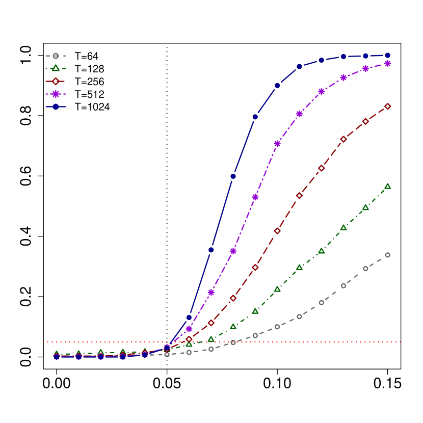
  ((a))

  

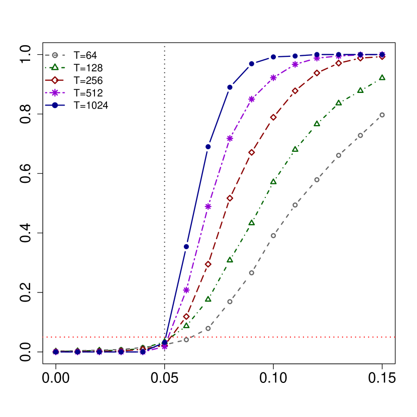
  ((b))

  

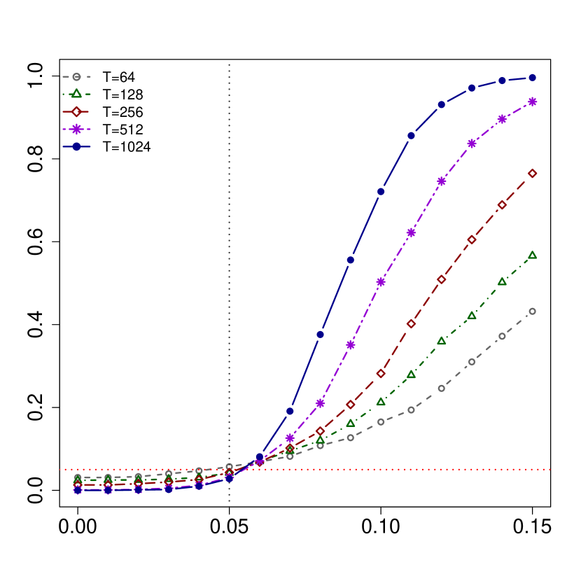
  ((c))

  Figure 4.1: ERP under scenario 1 of the relevant hypotheses tests (3.20) (panel (a)) and (3.28) for $k=1,2$ (panel (b)–(c), resp.) plotted as a function of $\iota$ at the nominal level 0.05 (horizontal dotted line). The true shift $\iota=0.05$ is marked in the three panels by the vertical dotted line and corresponds to induced threshold values $\Delta\approx 0.00047$, $\Delta_{\Pi,1}\approx 0.047$ and $\Delta_{\Pi,2}\approx 0.040$, respectively.

  

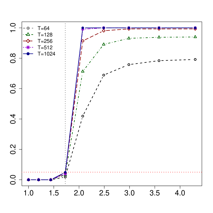
  ((a))

  

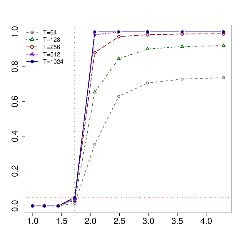
  ((b))

  

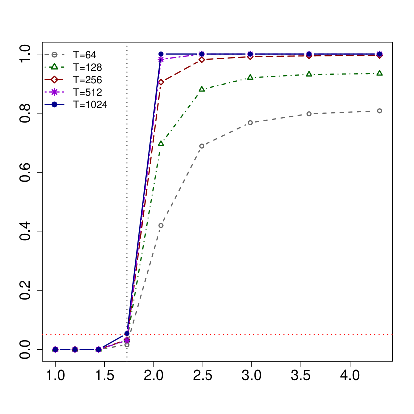
  ((c))

  Figure 4.2: ERP under scenario 2 of the relevant hypotheses tests (3.20) (panel (a)) and (3.31) for $k=1,2$ (panel (b)–(c), resp.) plotted as a function of $\iota$ at the nominal level 0.05 (horizontal dotted line). The true amplitude factor $\iota=1.2^{3}$ is marked by the vertical dotted line and corresponds to induced threshold values $\Delta\approx 0.044$, $\Delta_{\lambda,1}\approx 0.040$ and $\Delta_{\lambda,2}\approx 0.0025$, respectively.

• Scenario 2: amplitude variation. The alternative processes $\{Y_{t}\}^{T}_{t=1}$ are now generated as sequences from independent Brownian bridges where the standard deviation is multiplied by a factor $\iota=1.2^{\ell}\times\sqrt{2\pi},\ell=0,1,\ldots 8$. We consider a true factor $\iota=1.2^{3}$. Figure 4.2 provides the corresponding ERP of the test (3.20) in Section 3.1 (difference between operators, panel (a)) and of the test (3.31) in Section 3.3 (difference between eigenvalues for $k=1,2$, panel (b)–(c), resp.) Similar observations as in the previous scenario allow to conclude that the tests behave according to the derived theory, where the precision is quite accurate, even for the smaller sample sizes.

Setting B: Functional moving average. Next, we consider processes of the form

$$X_{t}=\sum_{s=0}^{2}A_{s}(\epsilon_{t-s})$$

where $\{\epsilon_{t}\}$ is a collection of independent Brownian motions on $[0,1]$. It is well known that $\epsilon_{t}$ can be represented using its KL expansion $\epsilon_{t}(\tau)=\sum_{k=1}^{\infty}\zeta_{k,t}e_{k}(\tau)$ where $\{\zeta_{k,t}\}_{k\geq 1}$ is a sequence of independent Gaussian random variables with variance $\text{var}(\zeta_{k,t})=\frac{1}{(k-1/2)^{2}\pi^{2}}$, and where the sequence $\{e_{k}\}_{k\geq 1}$ with $e_{k}(\tau)=\sqrt{2}\sin\big{(}(k-1/2)\pi\tau\big{)}$, $\tau\in[0,1]$, forms an orthonormal system of $L^{2}([0,1])$. We represent the operators $A_{s}$ in the basis $\{\psi_{l}\otimes e_{k}\}^{d,m}_{l=1,k=1}$, where we recall that $\{\psi_{l}\}$ denotes the Fourier basis on $[0,1]$. The vectors of coefficients $\tilde{X_{t}}=(\langle X_{t},\psi_{1}\rangle,\ldots,\langle X_{t},\psi_{d}\rangle)^{\top}$ can then be represented as

$$\tilde{X_{t}}=\sum_{s=0}^{2}\sum_{k=1}^{m}\tilde{A}_{s,(\cdot)k}\zeta_{k,t-s}=\sum_{s=0}^{2}\tilde{{A}}_{s}\bm{\zeta}_{t-s}.$$

We set $d=15,m=51$ and simulate the matrices $\tilde{{A}}_{s}=\{\tilde{A}_{s,lj}\}_{l,j}$ from a Gaussian distribution with independent entries such that $\tilde{A}_{0,lk}\sim\mathcal{N}(0,1)$, $\tilde{A}_{1,lj}\sim\mathcal{N}(0,(l+j^{3/2})^{-1})$, and $\tilde{A}_{2,lj}\sim\mathcal{N}(0,l^{-2})$.

• 

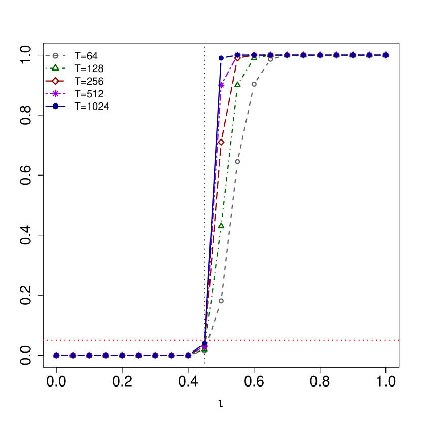
  ((a))

  

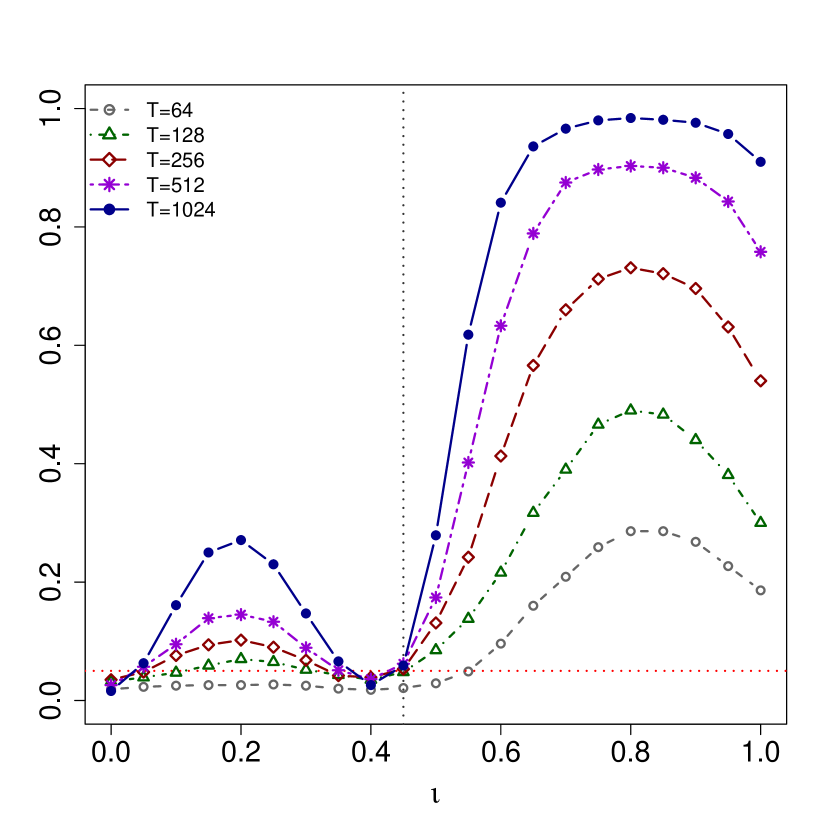
  ((b))

  Figure 4.3: ERP under scenario 3 for the relevant hypotheses tests (3.28) (panel (a)) and (3.31) (panel (b)) for $k=1$ plotted as a function of the parameter $\iota$ at the nominal level $0.05$ (horizontal dotted line). The vertical dotted line illustrates the true shift $\iota=0.45$. The induced thresholds values for $[a,b]=[0,\pi]$ are $\Delta_{\Pi,1}\approx 0.24$ and $\Delta_{\lambda,1}\approx 0.03$, respectively.

  

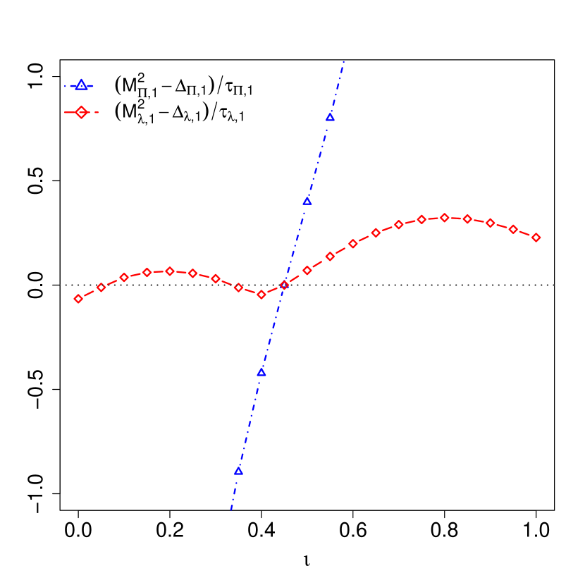
  ((a))

  

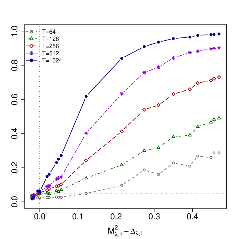
  ((b))

  Figure 4.4: Panel (a): the “relative” differences $(M^{2}_{\Pi,1}-\Delta_{\Pi,1})/\tau_{\Pi}$ and $(M^{2}_{\lambda,1}-\Delta_{\Pi,1})/\tau_{\lambda}$ in scenario 3. Panel (b): ERP as a function of $M^{2}_{\lambda,1}-\Delta_{\lambda,1}$, where the vertical dotted lines corresponds to $M^{2}_{\lambda,1}=\Delta_{\lambda,1}$.

  Scenario 3: shift in the eigenfunctions. We simulate $\{X_{t}\}_{t=1}^{T}$ and the alternative processes $\{Y_{t}\}_{t=1}^{T}$ from (4) , but for the alternative processes $\{Y_{t}\}_{t=1}^{T}$ we change the first eigenfunction of the innovations $\{\epsilon_{t}\}$ to ${e}_{1}(\tau)=\sqrt{2}\sin\big{(}(1/2+\iota)\pi\tau\big{)},\tau\in[0,1]$, where $\iota$ varies from $0$ to $1$. This shift affects various aspects of the second order structure non-uniformly over the frequency band, and most prominently the first order marginal characteristics. We therefore concentrate on testing relevant hypotheses for the largest eigenvalues and corresponding eigenprojectors on $[a,b]=[0,\pi]$. We let $\iota=0.45$ be the true value. This choice corresponds to the threshold $\Delta_{\Pi,1}\approx 0.24$ in (2.2) and $\Delta_{\lambda,1}\approx 0.02$ in (2.3). In Figure 4.3(a), we depict the ERP of the test (3.28) for the hypothesis of no relevant differences between the first eigenprojectors (Theorem 3.5), while the results corresponding to the test (3.31) for the hypothesis of no relevant differences between the largest eigenvalues (Theorem 3.7) can be found in Figure 4.3(b). Both the test for the first eigenprojector (a) and the test for the largest eigenvalue (b) closely align with the derived theory, but this statement needs a little more explanation.
  First, note that in the model under consideration it is not immediately clear that the distances $M^{2}_{\lambda,1}-\Delta_{\lambda,1}$ and $M^{2}_{\Pi,1}-\Delta_{\Pi,1}$ are monotone function of the parameter $\iota$. Therefore, we display in Figure 4.4(a) the “relative” differences $(M^{2}_{\lambda,1}-\Delta_{\lambda,1})/\tau_{\lambda}$ and $(M^{2}_{\Pi,1}-\Delta_{\Pi,1})/\tau_{\Pi}$ as a function of $\iota$, where $\tau_{\lambda}$ and $\tau_{\Pi}$ are the standard deviations appearing in the limiting processes (3.26) and (3.30), respectively. Note again that the choice $\iota=0.45$ corresponds to the boundary of the null hypothesis, that is $M^{2}_{\Pi,1}-\Delta_{\Pi,1}\approx 0$, $M^{2}_{\lambda,1}-\Delta_{\lambda,1}\approx 0$. We observe that the null hypothesis $H_{0}:M^{2}_{\Pi,1}\leq\Delta_{\Pi,1}$ is equivalent to $H_{0}:\iota\leq 0.45$. Moreover, a similar argument as in (3.21) shows that for large sample sizes the power of the test is approximately given by

  $$\mathbb{P}\Big{(}\mathbb{D}>-{\sqrt{b_{1}T_{1}+b_{2}T_{2}}\over\mathbb{V}}\cdot{M^{2}-\Delta\over\tau}+q_{1-\alpha}(\mathbb{D})\Big{)}~{},$$ (4.1)

  where $(M^{2}-\Delta)/\tau=(M^{2}_{\Pi,1}-\Delta_{\Pi,1})/\tau_{\Pi}$ for the test (3.28) (eigenprojectors) and $(M^{2}-\Delta)/\tau=(M^{2}_{\lambda,1}-\Delta_{\lambda,1})/\tau_{\lambda}$ for the test (3.31) (eigenvalues). Thus, the rejection probability depends (approximately) on the size of the relative difference $(M^{2}-\Delta)/\tau$ and a larger value means more power. Consequently, for the hypothesis of no relevant difference between the eigenprojectors, formula (4.1) indicates that for large sample sizes the power of the test (3.28) is a strictly increasing function of $\iota$ and this property is confirmed by the ERP displayed in Figure 4.3(a).
  On the other hand, from Figure 4.4(a) we also observe that the distance $(M^{2}_{\lambda,1}-\Delta_{\lambda,1})/\tau_{\lambda}$ is not a monotone function of the parameter $\iota$. In fact, most values of $\iota\in[0,1]$ represent the alternative $H_{1}:M^{2}_{\lambda,1}>\Delta_{\lambda,1}$ and only small neighbourhoods at $0$ and $0.45$ correspond to the null hypothesis. Consequently, Figure 4.3(b) mainly displays ERP under the alternative, which explains the fact that the simulated rejection probabilities exceed the nominal level for most $\iota\in[0,1]$ (note also that for $M^{2}_{\lambda,1}-\Delta_{\lambda,1}\approx 0$ the level is well approximated). The approximation for the power in formula (4.1) also provides an explanation for the non-monotonicity of the ERP in Figure 4.3(b). Additionally, we can use formula (4.1) for an heuristic explanation why the test (3.28) for the eigenprojectors has more power than the test (3.31) for the eigenvalues (compare Figure 4.3)(a) and (b)). Observe in Figure 4.4(a) that for $\iota>0.45$ the curve $(M^{2}_{\Pi,1}-\Delta_{\Pi,1})/\tau_{\Pi}$ exceeds the curve $(M^{2}_{\lambda,1}-\Delta_{\lambda,1})/\tau_{\lambda}$, which explains the (substantially) larger power of the test for the eigenprojectors.
  Finally, we also plot in panel (b) of Figure 4.4 the ERP of the test (3.31) against the differences $M^{2}_{\lambda,1}-\Delta_{\lambda,1}$ and observe that this test behaves according to the derived theory: i) the ERP converge to zero in the interior of the null hypothesis $M^{2}_{\lambda_{1}}<\Delta_{\lambda,1}=0.02$ ii) the ERJP converge to the nominal level at the boundary of the null hypothesis, i.e., where $M^{2}_{\lambda_{1}}\approx\Delta_{\lambda_{1}}$, and (iii) for those values belonging to the alternative hypothesis $M^{2}_{\lambda_{1}}>\Delta_{\lambda_{1}}$ power increases to $1$.

• Scenario 4: amplitude variation. Consider again the FMA(2) process as specified in (4). We now simulate $\{X_{t}\}_{t=1}^{T}$ and $\{Y_{t}\}_{t=1}^{T}$ from this process, but the variance of the noise process of the alternative processes $\{Y_{t}\}_{t=1}^{T}$ is multiplied with a factor $\iota=1.05^{\ell}$ where $\ell=0,\ldots,20$, that is, $\text{var}(\zeta_{k,t})=\frac{\iota}{((k-1/2)\pi)^{2}}$. We consider a true factor $\iota=1.05^{9}$ and $[a,b]=[0,\pi]$. The eigenprojectors are not affected by this change. Therefore, we display in Figure 4.5 the ERP of the test (3.20) in Section 3.1 (difference between operators, panel (a)) and of the test (3.31) in Section 3.3 (difference between eigenvalues for $k=1,2$, panel (b)–(c)). The effect of this change in amplitude is in fact almost fully captured by the sequences of largest eigenvalues. This is also what one may observe in panel (a) and (b), where the ERP of the test for the spectral density operators and of the test for the largest eigenvalues follow a similar pattern.

  

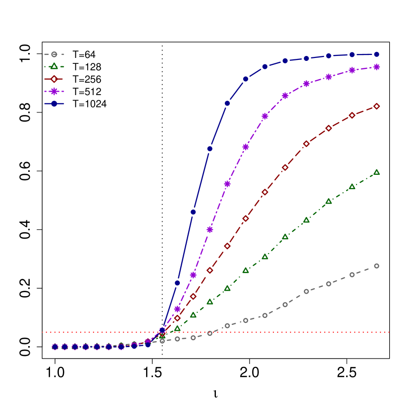
  ((a))

  

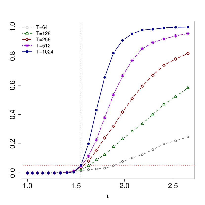
  ((b))

  

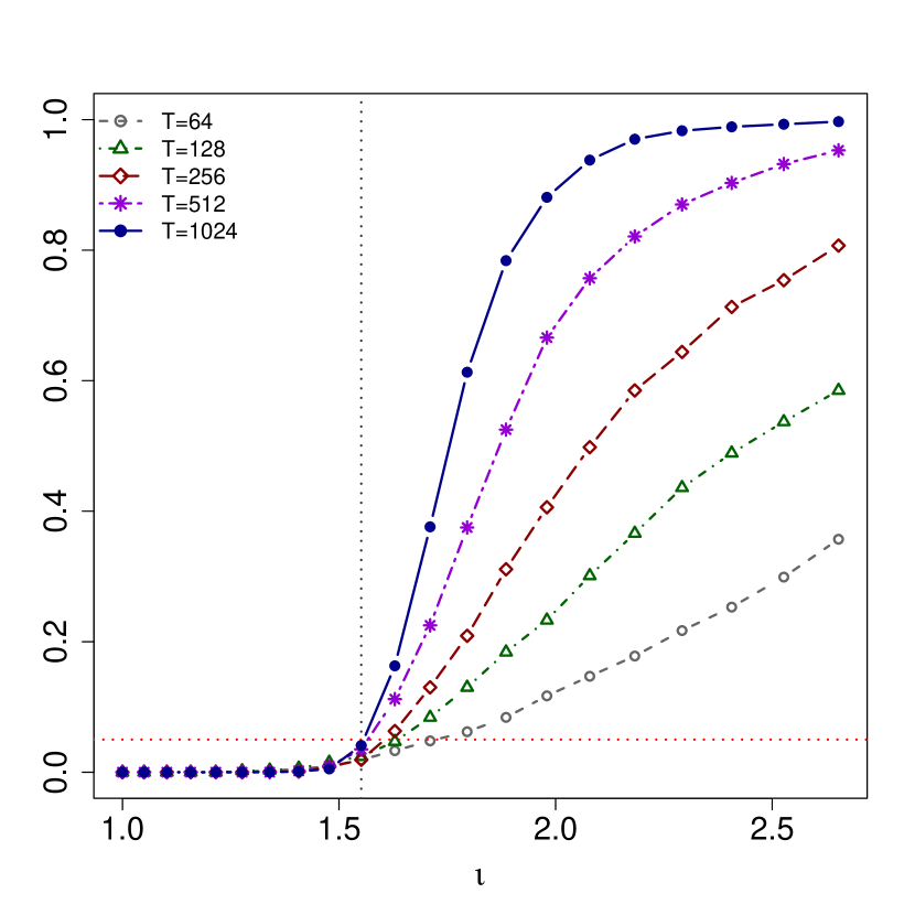
  ((c))

  Figure 4.5: ERP under scenario 4 for the relevant hypotheses tests (3.20) (panel (a)) and (3.31) for $k=1,2$ (panel (b)–(c), resp.) as a function of $\iota$ at the nominal level 0.05 (horizontal dotted line). The vertical dotted line illustrates the true factor $\iota=1.05^{9}$. The induced thresholds values for $[a,b]=[0,\pi]$ are $\Delta\approx 0.610$, $\Delta_{\lambda,1}\approx 0.605$ and $\Delta_{\lambda,2}\approx 0.004$, respectively.

Setting C: Functional autoregressive processes. Finally, we investigate finite sample performance in the context of functional AR(p) models

$$X_{t}=\sum_{j=1}^{p}A_{j}(X_{t-j})+\epsilon_{t},$$

where $A_{j}\in S_{\infty}(\mathcal{H})$ and $\{\epsilon_{t}\}_{t\in\mathbb{Z}}\in\mathcal{L}^{2}_{\mathcal{H}}$. A basis expansion yields that the first $d$ coefficients $\widetilde{X}_{t}=\left(\langle X_{t},\psi_{1}\rangle,\dots,\langle X_{t},\psi_{d}\rangle\right)^{\top}$ approximately satisfy the VAR(p) equation $\widetilde{{X}}_{t}=\sum_{j=1}^{p}\widetilde{A}_{j}(\widetilde{X}_{t-j})+\widetilde{\bm{\epsilon}}_{t}$ where $\widetilde{\epsilon}_{t}=\left(\langle\epsilon_{t},\psi_{1}\rangle,\dots,\langle\epsilon_{t},\psi_{d}\rangle\right)^{T}$ and where the $(l,l^{\prime})$-th entry of $\tilde{{A}}_{j}$ is given by $\langle A_{j}(\psi_{l}),\psi_{l^{\prime}}\rangle$. To ensure that the $A_{j}$ are bounded operators, we require that $\widetilde{A}_{j,l,l^{\prime}}\to 0$ as $l,l^{\prime}\to\infty$. To this end, the entries of the matrix $\widetilde{A}_{j}$ are generated as mutually independent $\mathcal{N}\big{(}0,\nu_{l,l^{\prime}}\big{)}$ with $\nu_{l,l^{\prime}}=\exp{(-i-j)}$. We fix $p=2$, $d=15$ and set $\widetilde{A}_{j}=\kappa_{j}\widetilde{A}_{j}/\rvert\rvert\rvert{\widetilde{A}_{j}}\rvert\rvert\rvert_{\infty},j=1,2$. The function-valued innovations $\epsilon_{1},\dots,\epsilon_{T}$ are i.i.d. Gaussian with coefficient variances $\text{Var}(\langle\epsilon_{t},\psi_{l}\rangle)=2\pi\exp(-l),l=1,\ldots,d$. Results are again provided for $[a,b]=[0,\pi]$.

• Scenario 5: amplitude variation. The processes $\{X_{t}\}_{t=1}^{T}$ are generated from (4) with $\kappa_{1}=\kappa=0.7$ and $\kappa_{2}=0$. The alternative processes $\{Y_{t}\}_{t=1}^{T}$ are generated similarly but with $\text{Var}(\langle\epsilon_{t},\psi_{l}\rangle)=\iota\times 2\pi\exp(-l),l=1,\ldots,d$, where $\iota=1.1^{\ell},\ell=0,\ldots,15$. In Figure 4.6, we present the results for a true factor $\iota=1.1^{7}$. Panel (a) displays the corresponding ERP of the test (3.20) in Section 3.1 (difference between operators), whereas the ERP of the tests (3.31) in Section 3.3 (difference between eigenvalues for $k=1,2$) are given in panel (c) and (d), respectively. We again observe both good nominal levels and good power for sample sizes $T\geq 128$.

  

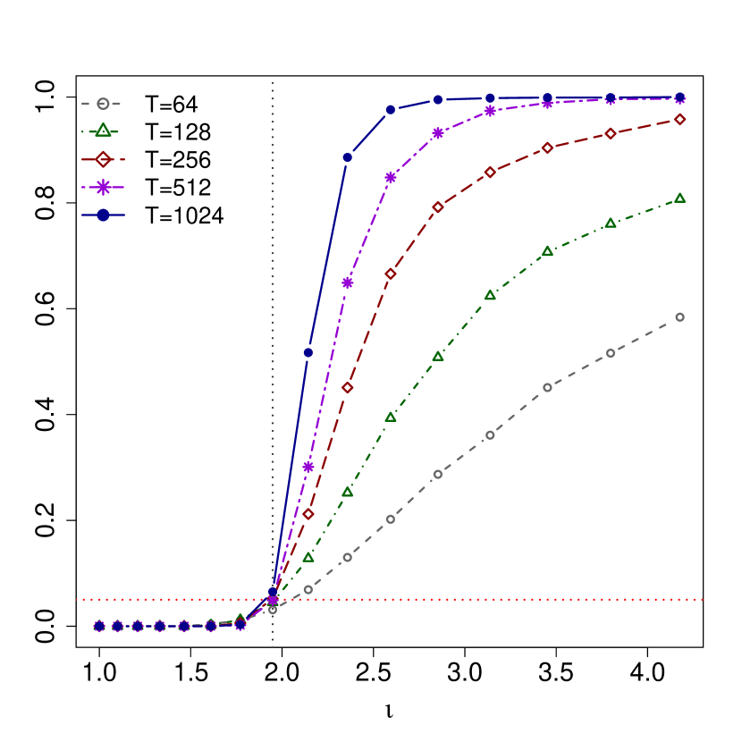
  ((a))

  

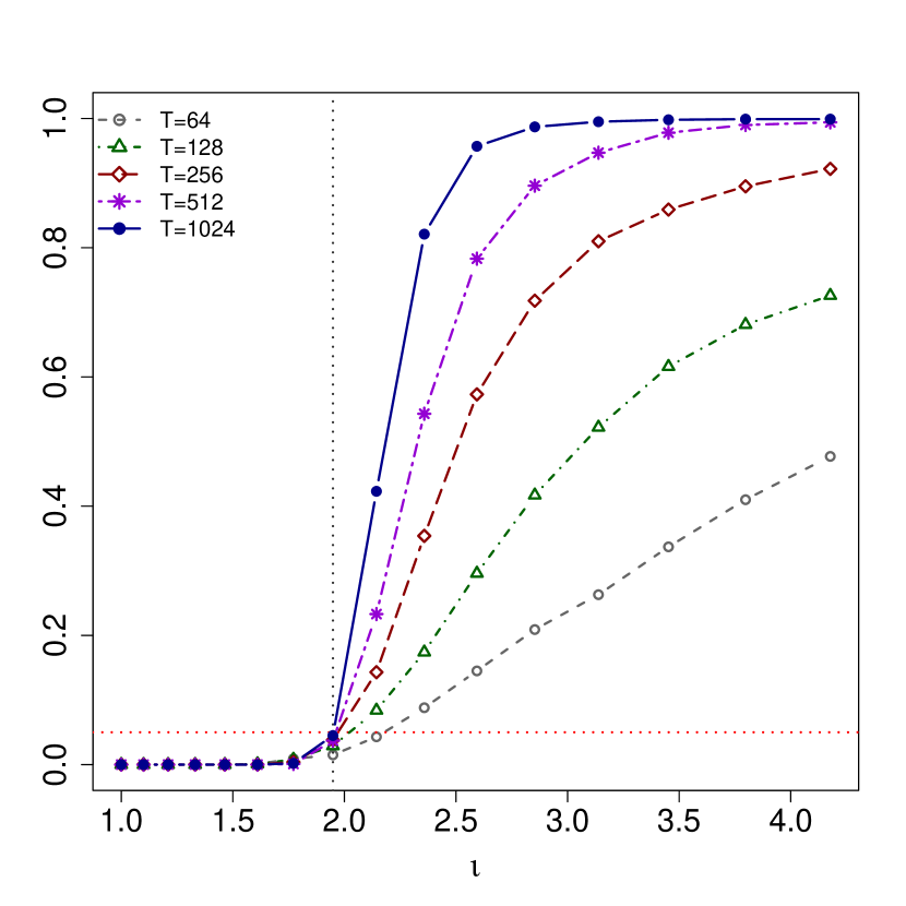
  ((b))

  

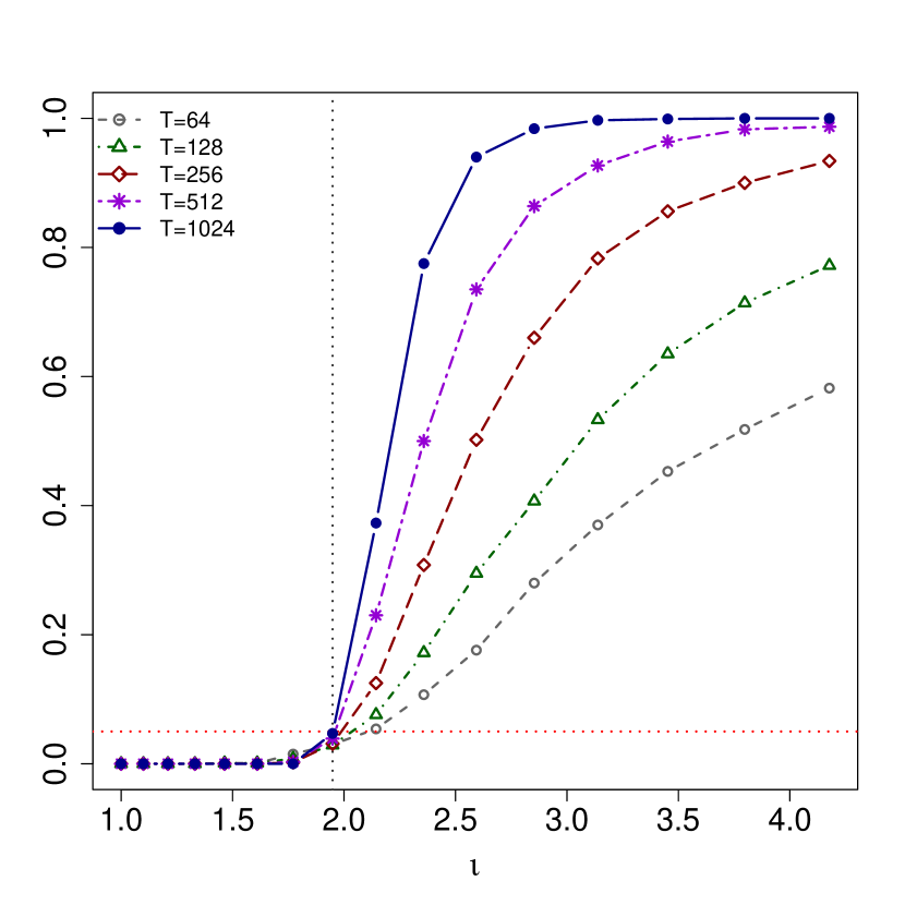
  ((c))

  Figure 4.6: ERP under scenario 5 for the relevant hypotheses tests introduced in Section 3.1 (a) and in Section 3.3 for $k=1,2$ ((b)–(c), resp.) as a function of $\iota$ at the nominal level 0.05 (horizontal dotted line). The vertical dotted line illustrates the true factor $\iota=1.1^{7}$, which induces thresholds for $[a,b]=[0,\pi]$ of $\Delta\approx 0.237$, $\Delta_{\lambda,1}\approx 0.213$, $\Delta_{\lambda,2}\approx 0.022$, respectively.

• Scenario 6: strength of dependence. The processes $\{X_{t}\}_{t=1}^{T}$ are again simulated from (4) with the introduced specifications and with $\kappa_{1}=0.75$ and $\kappa_{2}=0$. The alternative processes $\{Y_{t}\}_{t=1}^{T}$ are generated similarly, except that we vary the value of $\kappa_{2}$ from $0$ to $-0.75$. Note that this means that the models have strong dependence with complex dynamics and satisfy the existence of a causal solution in the weak sense that an appropriate power of the matrix of autoregressive operators in the state space representation has operator norm less than 1 (see e.g., section 3 in [10]). We let $\kappa_{2}=-0.2$ correspond to the boundary of the hypotheses. As illustrated in Figure 4.7(a), the effect on the relative differences between the true distances and induced thresholds is most dominantly visible in the first two eigenprojectors, the spectral density operators, and to a lesser extent in the largest eigenvalues. The corresponding ERP of the proposed tests of no relevant difference over $[a,b]=[0,\pi]$ for a hypothesized value of $\kappa_{2}=-0.2$ are provided in panel (b)–(e). It can be seen that the tests hold the nominal level well at the boundary of the null hypothesis (dotted vertical line) and power increases steadily at the interior of the alternative, which corroborates with theory. The power of the test for the largest eigenvalues (panel (e)) is smaller compared to those of the eigenprojectors (panel (c)–(d), resp.), which we can again explain by looking at the relative distances in Figure 4.7(a) and using the approximation (4.1). For the second eigenprojectors, the test is slightly oversized at the boundary which is most likely due to the fact that Assumption 3.5 is not completely satisfied over the entire frequency band. The slower convergence of the test for the largest eigenvalues can be explained by the fact that there are extremely fast changing dynamics over the frequency band, which also affects the test for the spectral density operators.

  

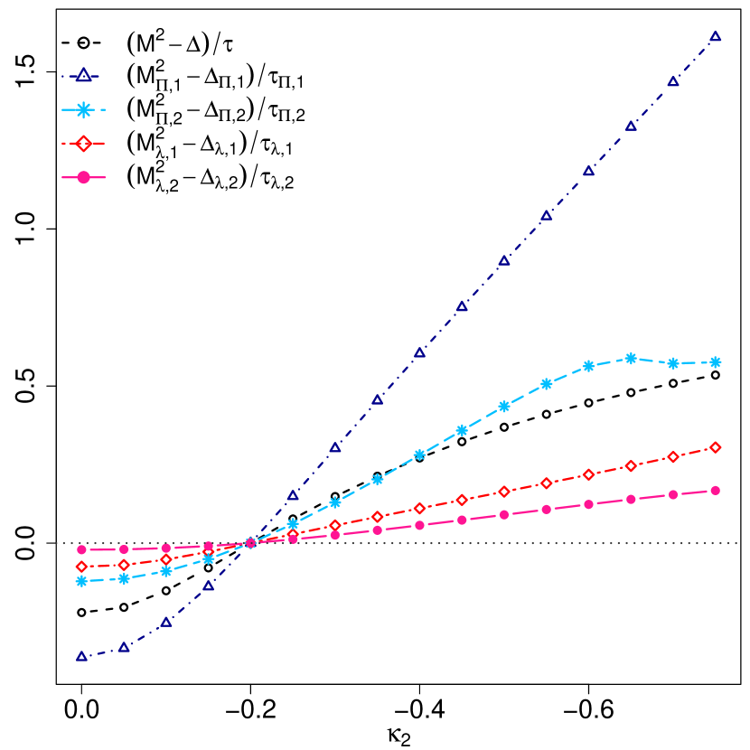
  ((a))

  

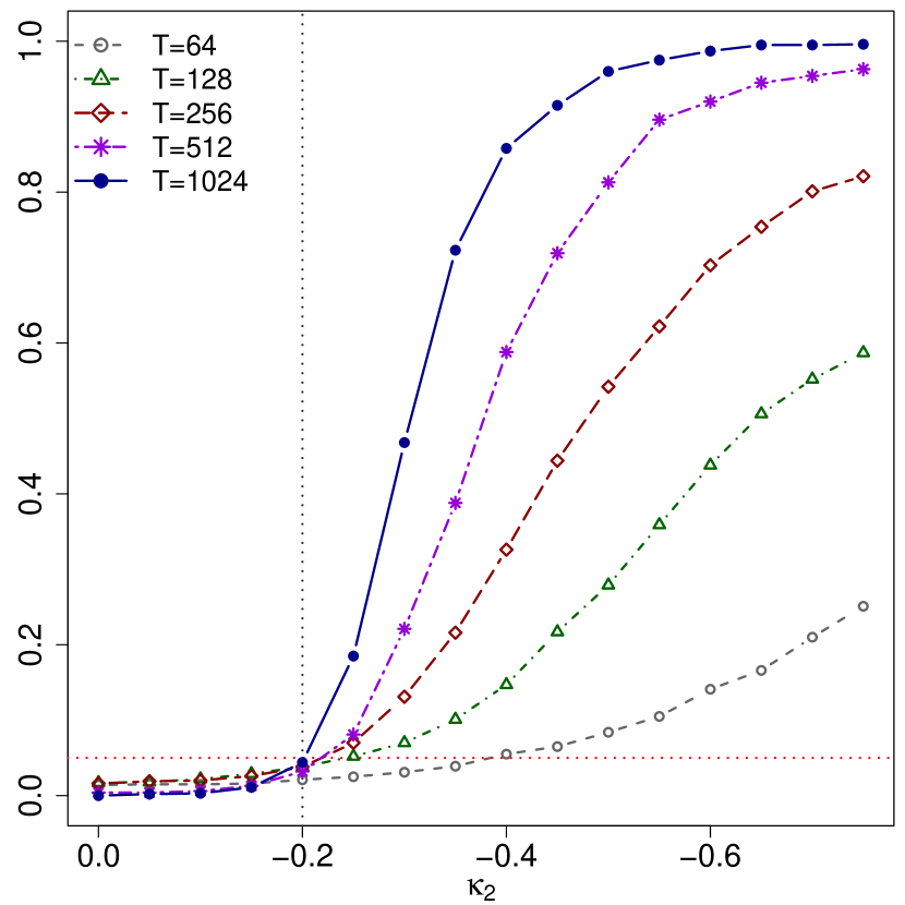
  ((b))

  

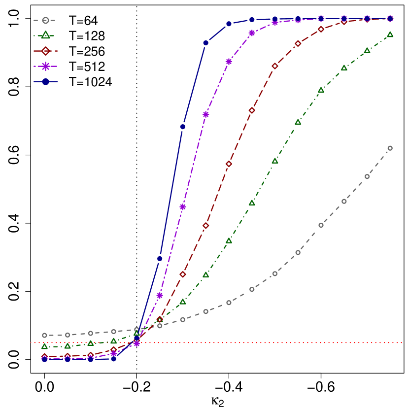
  ((c))

  

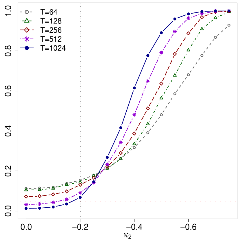
  ((d))

  

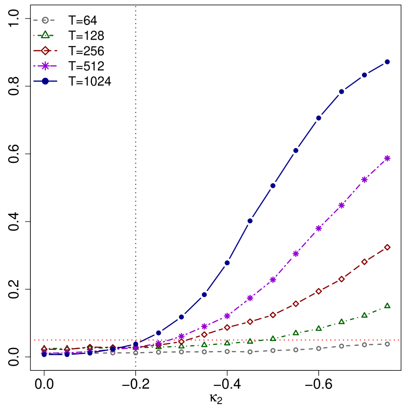
  ((e))

  Figure 4.7: Panel (a): the relative differences $(M^{2}-\Delta)/\tau$ and $(M^{2}_{\Pi,k}-\Delta_{\Pi,k})/\tau_{\Pi}$ and $(M^{2}_{\lambda,k}-\Delta_{\lambda,k})/\tau_{\lambda}$, for $k=1,2$ as a function of $\kappa_{2}$ under scenario 6. The value of $\kappa_{2}=-0.2$ (vertical dotted line) induces threshold values for $[a,b]=[0,\pi]$ of $\Delta\approx 0.024$, $\Delta_{\Pi,1}=0.0314$, $\Delta_{\Pi,2}=0.0444$, $\Delta_{\lambda,1}\approx 0.008$, $\Delta_{\lambda,2}\approx 0$. Panel ((b)–(e)): ERP under scenario 6 as a function of $\kappa_{2}$ at the nominal level 0.05 (horizontal dotted line) of the test (3.20) (panel (b)), of the test (3.28) for $k=1,2$ (panel (c)–(d), resp.), and of the test (3.31) for $k=1$ (panel (e)).

• Scenario 7: shift in the eigenfunctions. For this scenario, we consider functional autoregressive processes of the form (see also [25, 38, 3])

  $$X_{t}(\tau)=\sum_{j=1}^{2}\chi_{t,1,j}\sqrt{2}\sin(2\pi\tau j)+\chi_{t,2,j}\sqrt{2}\cos(2\pi(\tau j+\iota_{j})),\quad\tau\in[0,1],$$

  where the coefficients $\bm{\chi}_{t}=(\chi_{t,1,1},\chi_{t,2,1},\chi_{t,1,2},\chi_{t,2,2})$ are simulated from a vector autoregressive process, i.e., ${\bm{\chi}}_{t}=c\bm{\chi}_{t-1}+\sqrt{1-c^{2}}\epsilon_{t}$ with $\epsilon_{t}\in\mathbb{R}^{4}$. We generate $\{X_{t}\}^{T}_{t=1}$ from model (• ‣ 4) with $c=.7$, $\epsilon_{t}\in\mathbb{R}^{4}\sim\mathcal{N}(\bm{0},\mathrm{diag}(4,8,0.5,1.5))$, and $\iota_{j}=0,j=1,2$. The alternative processes $\{Y_{t}\}^{T}_{t=1}$ are simulated in the same way, except that the value of $\iota_{1}$ is varied between 0 and 0.25. In this model, higher degrees of persistence (i.e., larger values of $c$) lead to an increase of the relative contribution of the largest eigenvalues to the total variation, and to signal being concentrated in an increasingly narrow frequency band around zero, which results in violation of Assumption 3.5. Due to the strong persistence in this model for $c=0.7$, Assumption 3.5 is not satisfied over the entire frequency band $[0,\pi]$. In order to ensure that Assumption 3.5 is satisfied, we restrict the analysis to the interval $[a,b]=[0,\pi/4]$. We let $\iota=\iota_{1}=0.025$ be the shift factor that corresponds to the boundary of the hypotheses. The induced threshold values are $\Delta\approx 0.93$ $\Delta_{\Pi,1}=\Delta_{\Pi_{2}}\approx 0.17$, respectively. In Figure 4.8, we display the ERP of the test (3.20) in Section 3.1 (difference between operators, panel (a)) and of the test (3.28) in Section 3.2 (difference between projectors for $k=1,2$, panel ((b)–(c), resp.). The results closely align with theory. It is worth mentioning that for $\iota>0.2$, the relative difference $(M^{2}-\Delta)/\tau$ (as a function of $\iota$) exhibits a slight decline (similar to the phenomenon observed in scenario 3), the effect of which is discernible for the smaller sample sizes (see panel (a)).

  

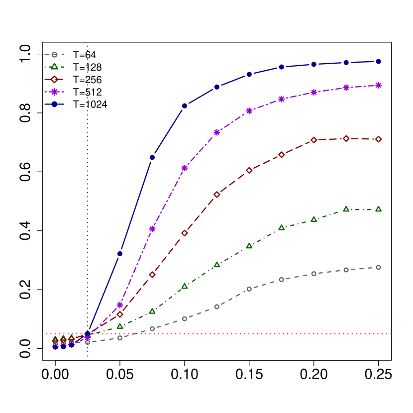
  ((a))

  

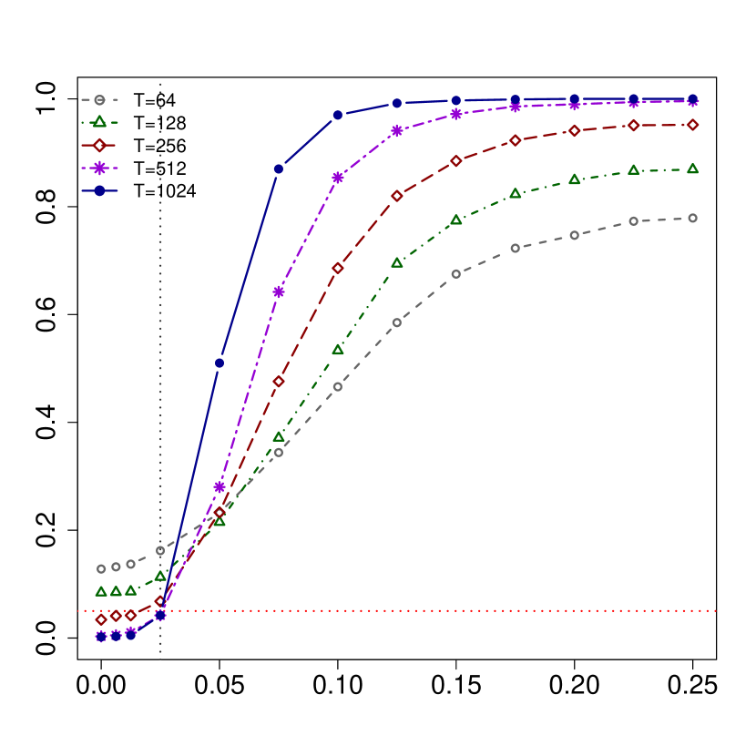
  ((b))

  

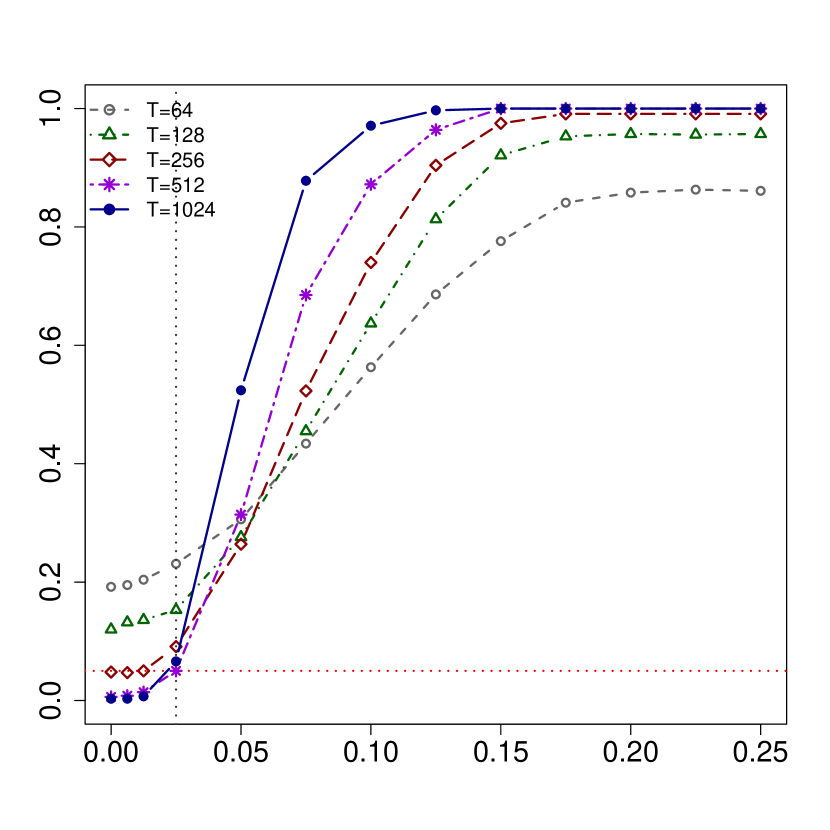
  ((c))

  Figure 4.8: ERP under scenario 7 as a function of $\iota$ at the nominal level 0.05 (horizontal dotted line) of the relevant hypotheses test (3.20) (panel (a)) and (3.28) for $k=1,2$ (panels (b)–(c), resp.). The vertical line illustrates the true shift factor $\iota=0.025$. The thresholds for $[a,b]=[0,\pi/4]$ induced by this shift are $\Delta\approx 0.93$, $\Delta_{\Pi,1}\approx\Delta_{\Pi,2}\approx 0.17$, respectively.

5 Proof of Theorem 3.1

In this section, we prove Theorem 3.1 and provide exact expressions of the constant $\tau_{XY}$ in terms of the spectral density operators and the factorizations of $\mathcal{U}^{(\omega)}_{XY}$ and $\mathcal{U}^{(\omega)}_{YX}$. We remark once more that the exact expression of $\mathcal{U}^{(\omega)}_{XY}$ depends on the specific hypothesis under consideration and that both are allowed to depend on both component processes $X$ and $Y$. In the following, consider

$$\mathcal{V}^{(\omega)}_{\bm{{X}}}=(\mathcal{V}^{(\omega)}_{X},\mathcal{V}^{(\omega)}_{Y})^{\top}$$ (5.1)

where $\mathcal{V}^{(\omega)}_{X},\mathcal{V}^{(\omega)}_{Y}$ are arbitrary elements of $S_{2}(\mathcal{H})$ and where the subscript only refers to the index of the component. Note that $\mathcal{V}^{(\omega)}_{\bm{{X}}}$ is an element of the Hilbert space $\mathscr{H}=S_{2}(\mathcal{H})\oplus S_{2}(\mathcal{H})$. In order to prove Theorem 3.1, we prove the following statement in detail.

Theorem 5.1.

Suppose Assumptions 3.1-3.4 are satisfied. Let $\mathcal{V}^{(\omega)}_{\bm{{X}}}\in\mathscr{H}$ be defined by (5.1), $\omega\in\mathbb{R}$, and define

$$\mathcal{Z}^{\bm{{X}},\omega}_{T,\eta}=\big{(}\mathcal{Z}^{X,\omega}_{T_{1},\eta}/\sqrt{b_{1}T_{1}},\mathcal{Z}^{Y,\omega}_{T_{2},\eta}/\sqrt{b_{2}T_{2}}\big{)}^{\top}\in\mathscr{H}$$

where $\mathcal{Z}^{X,\omega}_{T_{1},\eta}$ and $\mathcal{Z}^{Y,\omega}_{T_{2},\eta}$ are given by (3.2) and (3.3), respectively.

• If the component processes of $\{\bm{{X}}_{t}\}$ are dependent, then

  $$\Big{\{}\eta\sqrt{b_{1}T_{1}+b_{2}T_{2}}\Big{(}\int_{a}^{b}\Re\Big{(}\Big{\langle}\mathcal{Z}^{\bm{{X}},\omega}_{T,\eta},\mathcal{V}^{(\omega)}_{\bm{{X}}}\Big{\rangle}_{\mathscr{H}}\Big{)}d\omega\Big{\}}_{\eta\in[0,1]}\,{\rightsquigarrow}\,\Bigg{\{}\tau_{XY}\eta\,\mathbb{B}(\eta)\Bigg{\}}_{\eta\in[0,1]},$$

  where $\mathbb{B}$ is a Brownian motion, $\tau^{2}_{XY}=\frac{1}{4}\int^{b}_{a}\Re\Big{[}\Gamma^{\omega}_{\bm{{X}}}\big{(}\mathcal{V}^{(\omega)}_{\bm{{X}}}\big{)}+\Sigma^{\omega}_{\bm{{X}}}\big{(}\mathcal{V}^{(\omega)}_{\bm{{X}}}\big{)}\Big{]}d\omega$ with

  $$\Gamma^{\omega}_{\bm{{X}}}\big{(}\mathcal{V}^{(\omega)}_{\bm{{X}}}\big{)} =4\pi^{2}\sum_{l,j\in\{X,Y\}}\Big{(}\Big{\langle}\big{(}\mathcal{F}_{l,j}^{(\omega)}\widetilde{\otimes}\mathcal{F}_{j,l}^{\dagger(\omega)}\big{)}(\mathcal{V}^{(\omega)}_{j}),\mathcal{V}^{(\omega)}_{l}\Big{\rangle}_{S_{2}}+\mathrm{1}_{\omega\in\{0,\pi\}}\Big{\langle}\big{(}\mathcal{F}_{l,j}^{(\omega)}\widetilde{\otimes}\mathcal{F}_{j,l}^{\dagger(\omega)}\big{)}(\mathcal{V}^{(\omega)}_{j}),\overline{\mathcal{V}^{\dagger(\omega)}_{l}}\Big{\rangle}_{S_{2}}$$

  $$\phantom{\frac{1}{\mathcal{W}^{2}_{b_{T}}}}+\Big{\langle}\big{(}\mathcal{F}_{j,l}^{(\omega)}\widetilde{\otimes}\mathcal{F}_{l,j}^{\dagger(\omega)}\big{)}(\mathcal{V}^{\dagger(\omega)}_{l}),\mathcal{V}^{\dagger(\omega)}_{j}\Big{\rangle}_{S_{2}}+\mathrm{1}_{\omega\in\{0,\pi\}}\Big{\langle}\big{(}\mathcal{F}_{j,l}^{(\omega)}\widetilde{\otimes}\mathcal{F}_{l,j}^{\dagger(\omega)}\big{)}({\mathcal{V}^{(\omega)}_{j}}),\overline{(\mathcal{V}^{\dagger(\omega)}_{j}})\Big{\rangle}_{S_{2}}\Big{)}$$

  and

  $$\Sigma^{\omega}_{\bm{{X}}}\big{(}\mathcal{V}^{(\omega)}_{\bm{{X}}}\big{)} =4\pi^{2}\sum_{l,j\in\{X,Y\}}\Big{(}\mathrm{1}_{\omega\in\{0,\pi\}}\Big{(}\Big{\langle}\big{(}\mathcal{F}_{l,j}^{(\omega)}\widetilde{\otimes}\mathcal{F}_{j,l}^{\dagger(\omega)}\big{)}(\overline{\mathcal{V}^{(\omega)}_{j}}),\mathcal{V}^{(\omega)}_{l}\Big{\rangle}_{S_{2}}+\Big{\langle}\big{(}\mathcal{F}_{l,j}^{(\omega)}\widetilde{\otimes}\mathcal{F}_{j,l}^{\dagger(\omega)}\big{)}(\mathcal{V}^{\dagger(\omega)}_{j}),\mathcal{V}^{(\omega)}_{l}\Big{\rangle}_{S_{2}}$$

  $$+\mathrm{1}_{\omega\in\{0,\pi\}}\Big{\langle}\big{(}\mathcal{F}_{j,l,m}^{(\omega)}\widetilde{\otimes}\mathcal{F}_{l,j}^{\dagger(\omega)}\big{)}({\mathcal{V}^{\dagger(\omega)}_{l}}),\overline{\mathcal{V}^{\dagger(\omega)}_{j}}\Big{\rangle}_{S_{2}}+\Big{\langle}\big{(}\mathcal{F}_{j,l}^{(\omega)}\widetilde{\otimes}\mathcal{F}_{l,j}^{\dagger(\omega)}\big{)}({\mathcal{V}^{\dagger(\omega)}_{l}}),{\mathcal{V}^{(\omega)}_{j}}\Big{\rangle}_{S_{2}}\Big{)}$$

• If the component processes of $\{\bm{{X}}_{t}\}$ are independent, then

  $$\Big{\{}\eta\sqrt{b_{1}T_{1}+b_{2}T_{2}}\Big{(}\int_{a}^{b}\Re\Big{(}\Big{\langle}\mathcal{Z}^{\bm{{X}},\omega}_{T,\eta},\mathcal{V}^{(\omega)}_{\bm{{X}}}\Big{\rangle}_{\mathscr{H}}\Big{)}d\omega\Big{\}}_{\eta\in[0,1]}\,{\rightsquigarrow}\,\Bigg{\{}\eta\Big{(}\frac{\upsilon_{X}}{\sqrt{\theta}}\,\mathbb{B}_{X}(\eta)+\frac{\upsilon_{Y}}{\sqrt{1-\theta}}\,\mathbb{B}_{Y}(\eta)\Big{)}\Bigg{\}}_{\eta\in[0,1]}$$

  where $\mathbb{B}_{X}$ and $\mathbb{B}_{Y}$ are independent Brownian motions and $\upsilon^{2}_{l}=\frac{1}{4}\int^{b}_{a}\Re\Big{[}\Gamma^{\omega}_{l}\big{(}\mathcal{V}^{(\omega)}_{l}\big{)}+\Sigma^{\omega}_{l}\big{(}\mathcal{V}^{(\omega)}_{l}\big{)}\Big{]}d\omega$, $l\in\{X,Y\}$, with

  $$\Gamma^{(\omega)}_{l}(\mathcal{V}^{(\omega)}_{l}) ={4\pi^{2}}\Big{(}\Big{\langle}\big{(}\mathcal{F}_{l}^{(\omega)}\widetilde{\otimes}\mathcal{F}_{l}^{(\omega)}\big{)}(\mathcal{V}^{(\omega)}_{l}),\mathcal{V}^{(\omega)}_{l}\Big{\rangle}_{S_{2}}+\mathrm{1}_{\omega\in\{0,\pi\}}\Big{\langle}\big{(}\mathcal{F}_{l}^{(\omega)}\widetilde{\otimes}\mathcal{F}_{l}^{(\omega)}\big{)}(\mathcal{V}^{(\omega)}_{l}),\overline{\mathcal{V}^{\dagger(\omega)}_{l}}\Big{\rangle}_{S_{2}}$$

  $$\phantom{4\pi^{2}}+\Big{\langle}\big{(}\mathcal{F}_{l}^{(\omega)}\widetilde{\otimes}\mathcal{F}_{l}^{(\omega)}\big{)}(\mathcal{V}^{\dagger(\omega)}_{l}),\mathcal{V}^{\dagger(\omega)}_{l}\Big{\rangle}_{S_{2}}+\mathrm{1}_{\omega\in\{0,\pi\}}\Big{\langle}\big{(}\mathcal{F}_{l}^{(\omega)}\widetilde{\otimes}\mathcal{F}_{l}^{(\omega)}\big{)}({\mathcal{V}^{(\omega)}_{l}}),\overline{(\mathcal{V}^{\dagger(\omega)}_{l}})\Big{\rangle}_{S_{2}}\Big{)}$$

  and

  $$\Sigma^{(\omega)}_{l}(\mathcal{V}^{(\omega)}_{l})= 4\pi^{2}\Big{(}\mathrm{1}_{\omega\in\{0,\pi\}}\Big{(}\Big{\langle}\big{(}\mathcal{F}_{l}^{(\omega)}\widetilde{\otimes}\mathcal{F}_{l}^{(\omega)}\big{)}(\overline{\mathcal{V}^{(\omega)}_{l}}),\mathcal{V}^{(\omega)}_{l}\Big{\rangle}_{S_{2}}+\Big{\langle}\big{(}\mathcal{F}_{l}^{(\omega)}\widetilde{\otimes}\mathcal{F}_{l}^{(\omega)}\big{)}(\mathcal{V}^{\dagger(\omega)}_{l}),\mathcal{V}^{(\omega)}_{l}\Big{\rangle}_{S_{2}}$$

  $$\phantom{4\pi^{2}}+\mathrm{1}_{\omega\in\{0,\pi\}}\Big{\langle}\big{(}\mathcal{F}_{l}^{(\omega)}\widetilde{\otimes}\mathcal{F}_{l}^{(\omega)}\big{)}({\mathcal{V}^{\dagger(\omega)}_{l}}),\overline{\mathcal{V}^{\dagger(\omega)}_{l}}\Big{\rangle}_{S_{2}}+\Big{\langle}\big{(}\mathcal{F}_{l}^{(\omega)}\widetilde{\otimes}\mathcal{F}_{l}^{(\omega)}\big{)}({\mathcal{V}^{\dagger(\omega)}_{l}}),{\mathcal{V}^{(\omega)}_{l}}\Big{\rangle}_{S_{2}}\Big{)}.$$

Note that the expression for the covariance and pseudo-covariance in both parts of the statement can be further simplified if we further assume that the $\mathcal{V}^{(\omega)}_{l},l,j\in\{X,Y\}$ are self-adjoint, which is the case in all our statements.

Proof of Theorem 5.1.

The proof is involved and relies on several auxiliary results, which can be found in Appendix B. We will only prove part $i)$. The proof under independence follows similarly by verifying the steps for each component process separately and using the independence to conclude it for the linear combination. Using Assumption 3.4, we can ease notation in the dependent scenario and write $T=T_{1}=T_{2}$ throughout this section. Since we only assume very mild moment conditions, it is not obvious how to obtain the distributional properties directly. The principal idea is therefore to construct an approximating process of which the distributional properties can be established and then show that the process limiting distribution is the same as for the approximating process. Before we can introduce this process, we require some necessary terminology. Let

$$\bm{{X}}^{(m)}_{t}=\mathbb{E}[\bm{{X}}_{t}|\sigma(\epsilon_{t},\epsilon_{t-1},\ldots,\epsilon_{t-m})].$$

and define the $\mathcal{H}^{\oplus_{2}}$-valued stochastic process

$$D^{(\omega)}_{m,k}=(D^{(\omega)}_{X,m,k},D^{(\omega)}_{Y,m,k})^{\top}=\frac{1}{\sqrt{2\pi}}\sum_{t=0}^{\infty}\big{(}\mathbb{E}[\bm{{X}}^{(m)}_{t+k}|\mathcal{G}_{k}]-\mathbb{E}[\bm{{X}}^{(m)}_{t+k}|\mathcal{G}_{k-1}]\big{)}e^{-\mathrm{i}t\omega},$$

where $\mathcal{G}_{k}=\sigma(\epsilon_{k},\ldots\epsilon_{k-1},\ldots)$. Under Conditions A.1-A.2, this process is an $m$-dependent stationary martingale difference sequence w.r.t. the filtration $\{\mathcal{G}_{k}\}$ in $\mathcal{L}^{p}_{\mathcal{H}^{\oplus_{2}}}$ for each $\omega\in[-\pi,\pi]$. Additionally, consider a process defined by

$$\mathcal{M}^{{}(\omega)}_{T,m}=\sum_{t=2}^{T}\sum_{s=1}^{t-1}\tilde{w}^{(\omega)}_{b_{T},t,s}\mathcal{D}^{(\omega)}_{XY,s,t},$$ (5.3)

where $\mathcal{D}^{(\omega)}_{XY,s,t}=\Big{(}D^{(\omega)}_{X,m,t}\otimes D^{(\omega)}_{X,m,s},D^{(\omega)}_{Y,m,s}\otimes D^{(\omega)}_{Y,m,t}\Big{)}^{\top}$ and denote $\mathcal{W}^{2}_{b_{T}}=\sum_{t,s=1}^{T}|\tilde{w}^{(\omega)}_{b_{T},t,s}|^{2}$. Under Assumption 3.1, the process $\{\mathcal{W}^{-1}_{b_{T}}\mathcal{M}^{{}(\omega)}_{T,m}\}$ is a martingale in $\mathcal{L}^{p/2}_{\mathscr{H}}$ with respect to the filtration $\{\mathcal{G}_{T}\}$ for $p\geq 4$. The above claims on the properties of (5) and (5.3) can be verified similar to Proposition 3.2 and 3.3 of [3] by noting that for any $f=(f_{1},f_{2})^{\top}\in\mathscr{H}$, we have

$$\|f\|_{\mathscr{H}}=\rvert\rvert\rvert{f_{1}}\rvert\rvert\rvert_{S_{2}(\mathcal{H})}+\rvert\rvert\rvert{f_{2}}\rvert\rvert\rvert_{S_{2}(\mathcal{H})}$$

To construct the required approximating process, consider the arrays

$$N^{(\omega)}_{m,T,t}=\sum_{s=1}^{t-1}\Big{\langle}\tilde{w}^{(\omega)}_{b_{T},t,s}\mathcal{D}^{(\omega)}_{XY,s,t},\mathcal{V}^{(\omega)}_{\bm{{X}}}\Big{\rangle}_{\mathscr{H}}+\sum_{s=1}^{t-1}\Big{\langle}\Big{(}\tilde{w}^{(\omega)}_{b_{T},t,s}\mathcal{D}^{(\omega)}_{XY,s,t}\Big{)}^{\dagger},\mathcal{V}^{(\omega)}_{\bm{{X}}}\Big{\rangle}_{\mathscr{H}},\quad 2\leq t\leq T,$$

and set $N^{(\omega)}_{m,T,1}=0$ for all $\omega\in[-\pi,\pi]$. The following theorem provides the distributional properties of the (scaled) partial sum of the real part of (5) integrated over the frequency band $[a,b]$. The proof is involved and therefore postponed to Section A.3 of the supplement.

Theorem 5.2.

Let $N^{(\omega)}_{m,T,t}$ be defined as in (5) and let $\mathcal{{V}}^{(\omega)}_{\bm{{X}}}$ be defined as in (5.1). Suppose that Assumptions 3.1-3.3 hold. Then, for fixed $m$,

$$\frac{1}{\mathcal{W}_{b_{T}}}\Big{\{}\sum_{t=1}^{\lfloor\eta T\rfloor}\Re\Big{(}\int_{a}^{b}N^{(\omega)}_{m,T,t}d\omega\Big{)}\Big{\}}_{\eta\in[0,1]}\,\rightsquigarrow\,\tau_{m,XY}\cdot\Big{\{}\eta\mathbb{B}(\eta)\Big{\}}_{\eta\in[0,1]},\quad(T\to\infty)$$

where $\tau^{2}_{m,XY}=\frac{1}{4}\int^{b}_{a}\Re\Big{[}\Gamma^{\omega}_{\bm{{X}},m}\big{(}\mathcal{{V}}^{(\omega)}_{\bm{{X}}}\big{)}+\Sigma^{\omega}_{\bm{{X}},m}\big{(}\mathcal{{V}}^{(\omega)}_{\bm{{X}}}\big{)}\Big{]}d\omega$ with

$$\Gamma^{\omega}_{\bm{{X}},m}\big{(}\mathcal{{V}}^{(\omega)}_{\bm{{X}}}\big{)} =4\pi^{2}\sum_{l,j\in\{X,Y\}}\Big{\langle}\big{(}\mathcal{F}_{l,j,m}^{(\omega)}\widetilde{\otimes}\mathcal{F}_{j,l,m}^{\dagger(\omega)}\big{)}(\mathcal{V}^{(\omega)}_{j}),\mathcal{V}^{(\omega)}_{l}\Big{\rangle}_{S_{2}}+\mathrm{1}_{\omega\in\{0,\pi\}}\Big{\langle}\big{(}\mathcal{F}_{l,j,m}^{(\omega)}\widetilde{\otimes}\mathcal{F}_{j,l,m}^{\dagger(\omega)}\big{)}(\mathcal{V}^{(\omega)}_{j}),\overline{\mathcal{V}^{\dagger(\omega)}_{l}}\Big{\rangle}_{S_{2}}$$

$$\phantom{\frac{1}{\mathcal{W}^{2}_{b_{T}}}}+\Big{\langle}\big{(}\mathcal{F}_{j,l,m}^{(\omega)}\widetilde{\otimes}\mathcal{F}_{l,j,m}^{\dagger(\omega)}\big{)}(\mathcal{V}^{\dagger(\omega)}_{l}),\mathcal{V}^{\dagger(\omega)}_{j}\Big{\rangle}_{S_{2}}+\mathrm{1}_{\omega\in\{0,\pi\}}\Big{\langle}\big{(}\mathcal{F}_{j,l,m}^{(\omega)}\widetilde{\otimes}\mathcal{F}_{l,j,m}^{\dagger(\omega)}\big{)}({\mathcal{V}^{(\omega)}_{j}}),\overline{(\mathcal{V}^{\dagger(\omega)}_{j}})\Big{\rangle}_{S_{2}}$$

and

$$\Sigma^{\omega}_{\bm{{X}},m}\big{(}\mathcal{{V}}^{(\omega)}_{\bm{{X}}}\big{)} =4\pi^{2}\sum_{l,j\in\{X,Y\}}\Big{(}\Big{\langle}\big{(}\mathcal{F}_{l,j,m}^{(\omega)}\widetilde{\otimes}\mathcal{F}_{j,l,m}^{\dagger(\omega)}\big{)}(\mathcal{V}^{\dagger(\omega)}_{j}),\mathcal{V}^{(\omega)}_{l}\Big{\rangle}_{S_{2}}+\Big{\langle}\big{(}\mathcal{F}_{j,l,m}^{(\omega)}\widetilde{\otimes}\mathcal{F}_{l,j,m}^{\dagger(\omega)}\big{)}({\mathcal{V}^{\dagger(\omega)}_{l}}),{\mathcal{V}^{(\omega)}_{j}}\Big{\rangle}_{S_{2}}$$

$$\phantom{4\pi^{2}\sum_{l,j\in\{X,Y\}}}\mathrm{1}_{\omega\in\{0,\pi\}}\Big{\langle}\big{(}\mathcal{F}_{l,j,m}^{(\omega)}\widetilde{\otimes}\mathcal{F}_{j,l,m}^{\dagger(\omega)}\big{)}(\overline{\mathcal{V}^{(\omega)}_{j}}),\mathcal{V}^{(\omega)}_{l}\Big{\rangle}_{S_{2}}+\mathrm{1}_{\omega\in\{0,\pi\}}\Big{\langle}\big{(}\mathcal{F}_{j,l,m}^{(\omega)}\widetilde{\otimes}\mathcal{F}_{l,j,m}^{\dagger(\omega)}\big{)}({\mathcal{V}^{\dagger(\omega)}_{l}}),\overline{\mathcal{V}^{\dagger(\omega)}_{j}}\Big{\rangle}_{S_{2}}\Big{)},$$

and where $\mathcal{F}^{(\omega)}_{XY,m}=\mathbb{E}(D^{(\omega)}_{X,m,0}\otimes D^{(\omega)}_{Y,m,0})$.

We shall use Theorem 5.2 in order to derive the distributional properties of the process given in Theorem 5.1. We define

$${\widetilde{\mathcal{Z}}}^{\bm{{X}}}_{\lfloor\eta T\rfloor}=\eta\int^{b}_{a}{\widetilde{\mathcal{Z}}}^{\bm{{X}},\omega}_{\lfloor\eta T\rfloor}d\omega\quad\text{ and }\quad\widetilde{\mathcal{M}}^{\bm{{X}}}_{\lfloor\eta T\rfloor,m}=\frac{\eta}{\mathcal{W}_{b_{T}}}\sum_{t=1}^{\lfloor\eta T\rfloor}\int_{a}^{b}N^{(\omega)}_{m,T,t}d\omega$$

where

$${\widetilde{\mathcal{Z}}}^{\bm{{X}},\omega}_{\lfloor\eta T\rfloor} =\frac{1}{\mathcal{W}_{b_{T}}}\Big{\langle}\sum_{s=1}^{\lfloor\eta T\rfloor}\Big{(}\sum_{t=1}^{\lfloor\eta T\rfloor}\tilde{w}^{(\omega)}_{b_{T},s,t}(X_{s}\otimes X_{t},Y_{s}\otimes Y_{t})^{\top}-\mathbb{E}\big{(}\hat{\mathcal{F}}^{\omega}_{X}(\eta),\hat{\mathcal{F}}^{\omega}_{Y}(\eta)\big{)}^{\top}\Big{)},\mathcal{V}^{(\omega)}_{\bm{{X}}}\Big{\rangle}_{\mathscr{H}}.$$

Let $d_{S}$ denote the Skorokhod metric on $D[0,1])$ and $d_{U}$ the uniform metric and recall that $(D[0,1],d_{S})$ is a metric space. Let $F$ be a closed set of $D[0,1]$ and denote $F_{d_{S},\epsilon}=\big{\{}x:d_{S}\big{(}x,y\big{)}\leq\epsilon,y\in F\big{\}}$ Since the Skorokhod metric is weaker than the uniform metric, we have

$$\mathbb{P}\Big{(}\big{\{}\Re(\widetilde{\mathcal{Z}}^{\bm{{X}}}_{\lfloor\eta T\rfloor})\big{\}}_{\eta\in[0,1]}\in F\Big{)}$$

$$\leq\mathbb{P}\Big{(}d_{S}\big{(}\big{\{}\Re(\widetilde{\mathcal{Z}}^{\bm{{X}}}_{\lfloor\eta T\rfloor})\big{\}}_{\eta\in[0,1]},\big{\{}\Re(\widetilde{\mathcal{M}}^{\bm{{X}}}_{\lfloor\eta T\rfloor,m})\big{\}}_{\eta\in[0,1]}\big{)}\geq\epsilon\Big{)}+\mathbb{P}\Big{(}\big{\{}\Re(\widetilde{\mathcal{M}}^{\bm{{X}}}_{\lfloor\eta T\rfloor,m})\big{\}}_{\eta\in[0,1]}\in F_{d_{S},\epsilon}\Big{)}$$

$$\leq\mathbb{P}\Big{(}d_{U}\big{(}\big{\{}\Re(\widetilde{\mathcal{Z}}^{\bm{{X}}}_{\lfloor\eta T\rfloor})\big{\}}_{\eta\in[0,1]},\big{\{}\Re(\widetilde{\mathcal{M}}^{\bm{{X}}}_{\lfloor\eta T\rfloor,m})\big{\}}_{\eta\in[0,1]}\big{)}\geq\epsilon\Big{)}+\mathbb{P}\Big{(}\big{\{}\Re(\widetilde{\mathcal{M}}^{\bm{{X}}}_{\lfloor\eta T\rfloor,m})\big{\}}_{\eta\in[0,1]}\in F_{d_{S},\epsilon}\Big{)}$$

We will first prove that

$$\lim_{m\to\infty}\lim_{T\to\infty}\mathbb{P}\Big{(}d_{U}\big{(}\big{\{}\widetilde{\mathcal{Z}}^{\bm{{X}}}_{\lfloor\eta T\rfloor}\big{\}}_{\eta\in[0,1]},\big{\{}\widetilde{\mathcal{M}}^{\bm{{X}}}_{\lfloor\eta T\rfloor,m}\big{\}}_{\eta\in[0,1]}\big{)}\geq\epsilon\Big{)}=0.$$

By Markov’s inequality,

$$\mathbb{P}\Big{(}d_{U}\big{(}\big{\{}\widetilde{\mathcal{Z}}^{\bm{{X}}}_{\lfloor\eta T\rfloor}\big{\}}_{\eta\in[0,1]},\big{\{}\widetilde{\mathcal{M}}^{\bm{{X}}}_{\lfloor\eta T\rfloor,m}\big{\}}_{\eta\in[0,1]}\big{)}\geq\epsilon\Big{)}\leq\epsilon^{-\gamma}\mathbb{E}\Big{(}\sup_{\eta\in[0,1]}\Big{|}\widetilde{\mathcal{Z}}^{\bm{{X}}}_{\lfloor\eta T\rfloor}-\widetilde{\mathcal{M}}^{\bm{{X}}}_{\lfloor\eta T\rfloor,m}\Big{|}\Big{)}^{\gamma},$$

where we take $\gamma>2$. We find

$$\mathbb{E}\Big{(}\sup_{\eta\in[0,1]}\Big{|}\widetilde{\mathcal{Z}}^{\bm{{X}}}_{\lfloor\eta T\rfloor}-\widetilde{\mathcal{M}}^{\bm{{X}}}_{\lfloor\eta T\rfloor,m}\Big{|}\Big{)}^{\gamma} \leq\mathbb{E}\Big{(}\sup_{\eta\in[0,1]}\eta\int_{a}^{b}\Big{|}\Big{(}\widetilde{\mathcal{Z}}^{\bm{{X}},\omega}_{\lfloor\eta T\rfloor}-\frac{1}{\mathcal{W}_{b_{T}}}\sum_{t=1}^{\lfloor\eta T\rfloor}N^{(\omega)}_{m,T,t}\Big{)}\Big{|}d\omega\Big{)}^{\gamma}$$

$$\leq\mathbb{E}\Big{(}\int_{a}^{b}\sup_{\eta\in[0,1]}\eta\Big{|}\Big{(}\widetilde{\mathcal{Z}}^{\bm{{X}},\omega}_{\lfloor\eta T\rfloor}-\frac{1}{\mathcal{W}_{b_{T}}}\sum_{t=1}^{\lfloor\eta T\rfloor}N^{(\omega)}_{m,T,t}\Big{)}\Big{|}d\omega\Big{)}^{\gamma}$$

$$\leq(b-a)^{\gamma-1}\int_{a}^{b}\mathbb{E}\Big{(}\sup_{\eta\in[0,1]}\eta\Big{|}\Big{(}\widetilde{\mathcal{Z}}^{\bm{{X}},\omega}_{\lfloor\eta T\rfloor}-\frac{1}{\mathcal{W}_{b_{T}}}\sum_{t=1}^{\lfloor\eta T\rfloor}N^{(\omega)}_{m,T,t}\Big{)}\Big{|}\Big{)}^{\gamma}d\omega,$$ (5.7)

where the last inequality follows from an application of Jensen’s inequality to the integral since $\gamma>1$, and from Tonelli’s theorem, which allows to interchange the expectation and integral. Continuity of the Hilbert-Schmid inner product with respect to the product topology on $\mathcal{H}\otimes\mathcal{H}$ and the Cauchy-Schwarz inequality imply for the integrand of (5.7)

$$\mathbb{E}\Big{(}\sup_{\eta\in[0,1]}\eta\Big{|}\Big{(}\widetilde{\mathcal{Z}}^{\bm{{X}},\omega}_{\lfloor\eta T\rfloor}-\frac{1}{\mathcal{W}_{b_{T}}}\sum_{t=1}^{\lfloor\eta T\rfloor}N^{(\omega)}_{m,T,t}\Big{)}\Big{|}\Big{)}^{\gamma}$$

$$=\mathbb{E}\Big{(}\sup_{\eta}\eta\Big{|}\Big{\langle}\frac{1}{\mathcal{W}_{b_{T}}}\Big{(}\sum_{s=1}^{\lfloor\eta T\rfloor}\big{(}\sum_{t=1}^{\lfloor\eta T\rfloor}\tilde{w}^{(\omega)}_{b_{T},s,t}(X_{s}\otimes X_{t},Y_{s}\otimes Y_{t})^{\top}-\mathbb{E}\big{(}\hat{\mathcal{F}}^{\omega}_{X}(\eta),\hat{\mathcal{F}}^{\omega}_{Y}(\eta)\big{)}^{\top}\big{)}-\mathcal{M}^{{}(\omega)}_{\lfloor\eta T\rfloor,m}-\mathcal{M}^{{\dagger}(\omega)}_{\lfloor\eta T\rfloor,m}\Big{)},\mathcal{V}^{(\omega)}_{\bm{{X}}}\Big{\rangle}_{\mathscr{H}}\Big{|}\Big{)}^{\gamma}$$

$$\leq\big{(}\sup_{\omega}\rvert\rvert\rvert{\mathcal{V}^{(\omega)}_{\bm{{X}}}}\rvert\rvert\rvert^{\gamma}_{2}\big{)}\frac{1}{\mathcal{W}^{\gamma}_{b_{T}}}\mathbb{E}\Big{(}\sup_{\eta}\Big{\rvert}\Big{\rvert}\Big{\rvert}{\sum_{s=1}^{\lfloor\eta T\rfloor}\Big{(}\sum_{t=1}^{\lfloor\eta T\rfloor}\tilde{w}^{(\omega)}_{b_{T},s,t}(X_{s}\otimes X_{t},Y_{s}\otimes Y_{t})^{\top}-\mathbb{E}\big{(}\hat{\mathcal{F}}^{\omega}_{X}(\eta),\hat{\mathcal{F}}^{\omega}_{Y}(\eta)\big{)}^{\top}\Big{)}-\mathcal{M}^{{}(\omega)}_{\lfloor\eta T\rfloor,m}-\mathcal{M}^{{\dagger}(\omega)}_{\lfloor\eta T\rfloor,m}}\Big{\rvert}\Big{\rvert}\Big{\rvert}_{\mathscr{H}}\Big{)}^{\gamma},$$

where $\mathcal{M}^{{}(\omega)}_{\lfloor\eta T\rfloor,m}$ is defined in (5.3). (5) then follows from Lemma B.3 in the Appendix together with (5) and (5.7). Next, write the real part of a complex random variable as a linear combination with its conjugate and apply the triangle inequality to find

$$\mathbb{E}\Big{(}\sup_{\eta\in[0,1]}\Big{|}\Re(\widetilde{\mathcal{Z}}^{\bm{{X}},\omega}_{\lfloor\eta T\rfloor})-\Re(\mathcal{M}^{{}(\omega)}_{\lfloor\eta T\rfloor,m})\Big{|}\Big{)}^{\gamma} \leq\mathbb{E}\Big{(}\frac{1}{2}\sup_{\eta\in[0,1]}\Big{|}\widetilde{\mathcal{Z}}^{\bm{{X}},\omega}_{\lfloor\eta T\rfloor}-\mathcal{M}^{{}(\omega)}_{\lfloor\eta T\rfloor,m}\Big{|}+\frac{1}{2}\sup_{\eta\in[0,1]}\Big{|}\overline{\widetilde{\mathcal{Z}}^{\bm{{X}},\omega}_{\lfloor\eta T\rfloor}}-\overline{\mathcal{M}^{{}(\omega)}_{\lfloor\eta T\rfloor,m}}\Big{|}\Big{)}^{\gamma}$$

$$\leq\frac{1}{2}\mathbb{E}\Big{(}\sup_{\eta\in[0,1]}\Big{|}\widetilde{\mathcal{Z}}^{\bm{{X}},\omega}_{\lfloor\eta T\rfloor}-\mathcal{M}^{{}(\omega)}_{\lfloor\eta T\rfloor,m}\Big{|}\Big{)}^{\gamma}+\frac{1}{2}\mathbb{E}\Big{(}\sup_{\eta\in[0,1]}\Big{|}\overline{\widetilde{\mathcal{Z}}^{\bm{{X}},\omega}_{\lfloor\eta T\rfloor}}-\overline{\mathcal{M}^{{}(\omega)}_{\lfloor\eta T\rfloor,m}}\Big{|}\Big{)}^{\gamma}.$$

Using Lemma B.3 and (5.7) it then follows that

$$\lim_{m\to\infty}\lim_{T\to\infty}\mathbb{P}\Big{(}d_{U}\big{(}\big{\{}\Re(\widetilde{\mathcal{Z}}^{\bm{{X}}}_{\lfloor\eta T\rfloor})\big{\}}_{\eta\in[0,1]},\big{\{}\Re(\widetilde{\mathcal{M}}^{\bm{{X}}}_{\lfloor\eta T\rfloor,m})\big{\}}_{\eta\in[0,1]}\big{)}\geq\epsilon\Big{)}$$

$$\leq\lim_{m\to\infty}\lim_{T\to\infty}\epsilon^{-\gamma}(b-a)^{\gamma-1}\frac{1}{2}\int_{a}^{b}\Big{\{}\mathbb{E}\Big{(}\sup_{\eta\in[0,1]}\eta\Big{|}\widetilde{\mathcal{Z}}^{\bm{{X}},\omega}_{\lfloor\eta T\rfloor}-{\mathcal{M}}^{\bm{{X}},(\omega)}_{\lfloor\eta T\rfloor,m}\Big{|}\Big{)}^{\gamma}+\mathbb{E}\Big{(}\sup_{\eta\in[0,1]}\eta\Big{|}\overline{\widetilde{\mathcal{Z}}^{\bm{{X}},\omega}_{\lfloor\eta T\rfloor}}-\overline{{\mathcal{M}}^{\bm{{X}},(\omega)}_{\lfloor\eta T\rfloor,m}}\Big{|}\Big{)}^{\gamma}\Big{\}}d\omega=0,$$

which proves (5). Consequently, an application of Theorem 5.2 yields

$$\lim_{T\to\infty}\mathbb{P}\Big{(}\big{\{}\Re(\widetilde{\mathcal{Z}}^{X}_{\lfloor\eta T\rfloor})\big{\}}_{\eta\in[0,1]}\in F\Big{)} \leq\lim_{m\to\infty}\lim_{T\to\infty}\mathbb{P}\Big{(}\big{\{}\Re(\widetilde{\mathcal{M}}^{\bm{{X}}}_{\lfloor\eta T\rfloor,m})\big{\}}_{\eta\in[0,1]}\in F_{d_{S},\epsilon}\Big{)}$$

$$\leq\lim_{m\to\infty}\mathbb{P}\Bigg{(}\Big{\{}\tau_{m,XY}\cdot\mathbb{B}(\eta)\Big{\}}_{\eta\in[0,1]}\in F_{d_{S},\epsilon}\Bigg{)}$$

$$=\mathbb{P}\Bigg{(}\Big{\{}\tau_{XY}\cdot\mathbb{B}(\eta)\Big{\}}_{\eta\in[0,1]}\in F_{d_{S},\epsilon}\Bigg{)},$$

where the last equality follows by taking the limit with respect to $m$ of $\Gamma^{\omega}_{\bm{{X}},m}$ and $\Sigma^{\omega}_{\bm{{X}},m}$ to obtain the limiting covariance structure [see Proposition 3.2 of 3]. Taking $\epsilon\downarrow 0$, we obtain

$$\Big{\{}\Re(\widetilde{\mathcal{Z}}^{\bm{{X}}}_{\lfloor\eta T\rfloor})\Big{\}}_{\eta\in[0,1]}\,{\rightsquigarrow}\,\Bigg{\{}\eta{\tau_{XY}}\mathbb{B}(\eta)\Bigg{\}}_{\eta\in[0,1]}$$

Theorem 5.1 now follows from Lemma B.4 in the Appendix and from noting that

$$\Big{|}\frac{\sqrt{b_{T}}}{\sqrt{\kappa T}}-\frac{1}{\mathcal{W}_{b_{T}}}\Big{|} =\Big{|}\frac{\sqrt{b_{T}}}{\sqrt{\kappa T}}\frac{\mathcal{W}_{b_{T}}}{\mathcal{W}_{b_{T}}}-\frac{1}{\mathcal{W}_{b_{T}}}\Big{|}=\frac{1}{\mathcal{W}_{b_{T}}}\Big{|}\frac{\sqrt{b_{T}}}{\sqrt{\kappa T}}\Big{(}\frac{\sqrt{T\kappa}}{\sqrt{b_{T}}}(1+o(1))\Big{)}-1\Big{|}=o(\frac{1}{\mathcal{W}_{b_{T}}})=o(1),$$

where we used that under Assumption 3.2 $\mathcal{W}^{2}_{b_{T}}=\sum_{|h|<T}(T-|h|)w(b_{T}h)^{2}=\frac{T}{b_{T}}(\kappa+o(1))$. ∎

Appendix A Proofs of main statements

A.1 Proofs of statements from Section 3

Proof of Proposition 3.1.

This follows from an adjustment of the proof of Theorem 4.1(ii) of [3] for the value of $\ell$. Details are omitted. ∎

Proof of Lemma 3.1.

Using Tonelli’s theorem,

$$\mathbb{E}\Big{(}\sup_{\eta\in[0,1]}\int_{a}^{b}\Big{\rvert}\Big{\rvert}\Big{\rvert}{\widehat{M}_{\hat{\mathcal{F}}}(\eta,\omega)-\eta{M}_{\mathcal{F}}(\omega)}\Big{\rvert}\Big{\rvert}\Big{\rvert}^{2}_{2}d\omega\Big{)}\leq\int_{a}^{b}\mathbb{E}\Big{(}\sup_{\eta\in[0,1]}\Big{\rvert}\Big{\rvert}\Big{\rvert}{\widehat{M}_{\hat{\mathcal{F}}}(\eta,\omega)-\eta{M}_{\mathcal{F}}(\omega)}\Big{\rvert}\Big{\rvert}\Big{\rvert}^{2}_{2}\Big{)}d\omega$$

Observe that

$$\Big{\rvert}\Big{\rvert}\Big{\rvert}{\widehat{M}_{\hat{\mathcal{F}}}(\eta,\omega)-\eta{M}_{\mathcal{F}}(\omega)}\Big{\rvert}\Big{\rvert}\Big{\rvert}^{2}_{2}\leq 2\rvert\rvert\rvert{\eta\big{(}\hat{\mathcal{F}}_{X}^{(\omega)}(\eta)-\mathcal{F}_{X}^{(\omega)}\big{)}}\rvert\rvert\rvert^{2}_{2}+2\rvert\rvert\rvert{\eta\big{(}\hat{\mathcal{F}}^{(\omega)}_{Y}(\eta)-{\mathcal{F}}^{(\omega)}_{Y}\big{)}}\rvert\rvert\rvert^{2}_{2},$$

and that $\frac{\eta}{{\lfloor\eta T\rfloor}}=\frac{\eta T}{\eta T}\frac{\eta}{{\lfloor\eta T\rfloor}}=\frac{1}{T}\big{(}\frac{\eta T}{\lfloor\eta T\rfloor}-1\big{)}+\frac{1}{T}$. Jensen’s inequality and Minkowski’s inequality yield

$$\mathbb{E}\sup_{\eta\in[0,1]}\Big{\rvert}\Big{\rvert}\Big{\rvert}{\eta\big{(}\hat{\mathcal{F}}_{X}^{(\omega)}(\eta)-\mathcal{F}_{X}^{(\omega)}\big{)}}\Big{\rvert}\Big{\rvert}\Big{\rvert}^{2}_{2} {\leq\Big{(}\mathbb{E}\big{(}\sup_{\eta\in[0,1]}\Big{\rvert}\Big{\rvert}\Big{\rvert}{\frac{1}{T_{1}}\sum_{s=1}^{\lfloor\eta T_{1}\rfloor}\Big{(}\sum_{t=1}^{\lfloor\eta T_{1}\rfloor}\tilde{w}^{(\omega)}_{b_{1},s,t}(X_{s}\otimes X_{t})-\mathcal{F}_{X}^{(\omega)}\Big{)}}\Big{\rvert}\Big{\rvert}\Big{\rvert}_{2}\big{)}^{\gamma}\Big{)}^{2/\gamma}}$$

$${+\sup_{\eta\in[0,1]}\Big{|}\frac{\eta T}{\lfloor\eta T\rfloor}-1\Big{|}^{2}\Big{(}\mathbb{E}\big{(}\sup_{\eta\in[0,1]}\Big{\rvert}\Big{\rvert}\Big{\rvert}{\frac{1}{T_{1}}\sum_{s=1}^{\lfloor\eta T_{1}\rfloor}\Big{(}\sum_{t=1}^{\lfloor\eta T_{1}\rfloor}\tilde{w}^{(\omega)}_{b_{1},s,t}(X_{s}\otimes X_{t})-\mathcal{F}_{X}^{(\omega)}\Big{)}}\Big{\rvert}\Big{\rvert}\Big{\rvert}_{2}\big{)}^{\gamma}\Big{)}^{2/\gamma}}$$

$$=O(b^{-1}_{1}T_{1}^{-1})+O(b^{2\ell}_{1}).$$

where we used (B) and (B) and (B) as in the proof of Lemma B.1. In complete analogy, we obtain

$$\mathbb{E}\sup_{\eta\in[0,1]}\Big{\rvert}\Big{\rvert}\Big{\rvert}{\eta\big{(}\hat{\mathcal{F}}_{Y}^{(\omega)}(\eta)-\mathcal{F}_{Y}^{(\omega)}\big{)}}\Big{\rvert}\Big{\rvert}\Big{\rvert}^{2}_{2}=O(b^{-1}_{2}T_{2}^{-1})+O(b^{2\ell}_{2}).$$

The statement now follows from Assumption 3.3 and Assumption 3.4. ∎

Proof of Theorem 3.2.

This follows from Lemma 3.1 and Lemma B.2 and from using that $c\in\mathbb{C}$, $c+\overline{c}=2\Re(c)$.∎

Proof of Lemma 3.2.

Denote the perturbation $\hat{\Delta}_{\eta}\mathcal{F}^{\omega}=\hat{\mathcal{F}}^{\omega}(\eta)-\mathcal{F}^{\omega}$. We first consider $\mathrm{(i)}$. Observe that by Minkowski’s inequality it suffices to show

$$\sup_{\eta\in[0,1]} \int_{a}^{b}\eta\Bigg{\rvert}\Bigg{\rvert}\Bigg{\rvert}{\hat{\Pi}^{(\omega)}_{X,k}(\eta)-{\Pi}^{(\omega)}_{X,k}-\sum_{\begin{subarray}{c}j,j^{\prime}=1,\\ \{j,j^{\prime}=k\}^{\complement}\end{subarray}}^{\infty}\frac{\Big{\langle}\mathcal{F}_{X}^{(\omega)}\widetilde{\otimes}\hat{\Delta}_{\eta}\mathcal{F}_{X}^{(\omega)}+\hat{\Delta}_{\eta}\mathcal{F}_{X}^{(\omega)}\widetilde{\otimes}\mathcal{F}_{X}^{(\omega)},{\Pi}^{(\omega)}_{X,jj^{\prime}}\widetilde{\otimes}{\Pi}^{(\omega)}_{X,k}\Big{\rangle}_{S_{2}}{\Pi}^{(\omega)}_{X,jj^{\prime}}}{\lambda^{(\omega)}_{X,j}\lambda^{(\omega)}_{X,j^{\prime}}-(\lambda^{(\omega)}_{X,k})^{2}}}\Bigg{\rvert}\Bigg{\rvert}\Bigg{\rvert}_{2}d\omega$$

$$=O_{p}\Big{(}\frac{\log^{4/\gamma}(T_{1})}{b_{1}T_{1}}\Big{)}$$ (A.1)

and

$$\sup_{\eta\in[0,1]} \int_{a}^{b}\eta\Bigg{\rvert}\Bigg{\rvert}\Bigg{\rvert}{\hat{\Pi}^{(\omega)}_{Y,k}(\eta)-{\Pi}^{(\omega)}_{Y,k}-\sum_{\begin{subarray}{c}j,j^{\prime}=1,\\ \{j,j^{\prime}=k\}^{\complement}\end{subarray}}^{\infty}\frac{\Big{\langle}\mathcal{F}_{Y}^{(\omega)}\widetilde{\otimes}\hat{\Delta}_{\eta}\mathcal{F}_{Y}^{(\omega)}+\hat{\Delta}_{\eta}\mathcal{F}_{Y}^{(\omega)}\widetilde{\otimes}\mathcal{F}_{Y}^{(\omega)},{\Pi}^{(\omega)}_{Y,jj^{\prime}}\widetilde{\otimes}{\Pi}^{(\omega)}_{Y,k}\Big{\rangle}_{S_{2}}{\Pi}^{(\omega)}_{Y,jj^{\prime}}}{\lambda^{(\omega)}_{Y,j}\lambda^{(\omega)}_{Y,j^{\prime}}-(\lambda^{(\omega)}_{Y,k})^{2}}}\Bigg{\rvert}\Bigg{\rvert}\Bigg{\rvert}_{2}d\omega$$

$$=O_{p}\Big{(}\frac{\log^{4/\gamma}(T_{2})}{b_{2}T_{2}}\Big{)}.$$

As the proof for both processes is the same, we shall focus on (A.1) and drop the subscript $X$ in the following. From Proposition 3.2, we have

$$\hat{\Pi}^{(\omega)}_{k}-{\Pi}^{(\omega)}_{k} =\Big{\langle}\hat{\Pi}^{\omega}_{k}(\eta)-{\Pi}^{\omega}_{k},{\Pi}^{\omega}_{k}\Big{\rangle}\Pi^{(\omega)}_{k}$$

$$+\sum_{\begin{subarray}{c}j,j^{\prime}=1,\\ \{j,j^{\prime}=k\}^{\complement}\end{subarray}}^{\infty}\frac{1}{\lambda^{(\omega)}_{j}\lambda^{(\omega)}_{j^{\prime}}-(\lambda^{(\omega)}_{k})^{2}}\Big{[}\Big{\langle}\big{(}\mathcal{F}^{\omega}\widetilde{\otimes}\mathcal{F}^{\omega}-\hat{\mathcal{F}}^{\omega}(\eta)\widetilde{\otimes}\hat{\mathcal{F}}^{\omega}(\eta)\big{)}\Pi^{(\omega)}_{k},\Pi^{(\omega)}_{jj^{\prime}}\Big{\rangle}_{S_{2}}+\Big{\langle}E^{(\omega)}_{k,b_{T}}(\eta),\Pi^{(\omega)}_{jj^{\prime}}\Big{\rangle}_{S_{2}}\Big{]}\Pi^{(\omega)}_{jj^{\prime}},$$

where

$$E^{(\omega)}_{k,b_{T}}(\eta)=\Big{[}(\mathcal{F}^{\omega}\widetilde{\otimes}\mathcal{F}^{\omega}-\hat{\mathcal{F}}^{\omega}(\eta)\widetilde{\otimes}\hat{\mathcal{F}}^{\omega}(\eta))\Big{]}\Big{[}\hat{\Pi}^{(\omega)}_{k}-{\Pi}^{(\omega)}_{k}\Big{]}+\Big{[}\big{(}\lambda^{(\omega)}_{k}(\eta)\big{)}^{2}\ -\big{(}\lambda^{(\omega)}_{k}\big{)}^{2}\Big{]}\Big{[}\hat{\Pi}^{(\omega)}_{k}-{\Pi}^{(\omega)}_{k}\Big{]}.$$ (A.2)

Elementary calculations yield

$$\hat{\mathcal{F}}^{\omega}(\eta)\widetilde{\otimes}\hat{\mathcal{F}}^{\omega}(\eta)-\mathcal{F}^{\omega}\widetilde{\otimes}\mathcal{F}^{\omega} =\mathcal{F}^{\omega}\widetilde{\otimes}\big{(}\hat{\Delta}_{\eta}\mathcal{F}^{\omega}\big{)}+\big{(}\hat{\Delta}_{\eta}\mathcal{F}^{\omega}\big{)}\widetilde{\otimes}{\mathcal{F}}^{\omega}+\big{(}\hat{\Delta}_{\eta}\mathcal{F}^{\omega}\big{)}\widetilde{\otimes}\big{(}\hat{\Delta}_{\eta}\mathcal{F}^{\omega}\big{)}.$$

Therefore, we will show that

$$\sup_{\eta\in[0,1]}\eta\int_{a}^{b}\Bigg{\rvert}\Bigg{\rvert}\Bigg{\rvert}{\Big{\langle}\hat{\Pi}^{\omega}_{k}(\eta)-{\Pi}^{\omega}_{k},{\Pi}^{\omega}_{k}\Big{\rangle}_{S_{2}}\Pi^{(\omega)}_{k}+\sum_{\begin{subarray}{c}j,j^{\prime}=1,\\ \{j,j^{\prime}=k\}^{\complement}\end{subarray}}^{\infty}\frac{\Big{[}\Big{\langle}\hat{\Delta}_{\eta}\mathcal{F}^{\omega}\widetilde{\otimes}\hat{\Delta}_{\eta}\mathcal{F}^{\omega}\big{)}\Pi^{(\omega)}_{k},\Pi^{(\omega)}_{jj^{\prime}}\Big{\rangle}_{S_{2}}+\Big{\langle}E^{(\omega)}_{k,b_{T}}(\eta),\Pi^{(\omega)}_{jj^{\prime}}\Big{\rangle}_{S_{2}}\Big{]}\Pi^{(\omega)}_{jj^{\prime}}}{\lambda^{(\omega)}_{j}\lambda^{(\omega)}_{j^{\prime}}-(\lambda^{(\omega)}_{k})^{2}}}\Bigg{\rvert}\Bigg{\rvert}\Bigg{\rvert}_{2}d\omega$$

$$=O_{p}\Big{(}\frac{\log^{4/\gamma}(T_{1})}{b_{T_{1}}T_{1}}\Big{)}.$$

By Minkowski’s inequality,

$$\sup_{\eta\in[0,1]}\eta\int_{a}^{b}\Bigg{\rvert}\Bigg{\rvert}\Bigg{\rvert}{\Big{\langle}\hat{\Pi}^{\omega}_{k}(\eta)-{\Pi}^{\omega}_{k},{\Pi}^{\omega}_{k}\Big{\rangle}_{S_{2}}\Pi^{(\omega)}_{k}+\sum_{\begin{subarray}{c}j,j^{\prime}=1,\\ \{j,j^{\prime}=k\}^{\complement}\end{subarray}}^{\infty}\frac{\Big{[}\Big{\langle}\hat{\Delta}_{\eta}\mathcal{F}^{\omega}\widetilde{\otimes}\hat{\Delta}_{\eta}\mathcal{F}^{\omega}\big{)}\Pi^{(\omega)}_{k},\Pi^{(\omega)}_{jj^{\prime}}\Big{\rangle}_{S_{2}}+\Big{\langle}E^{(\omega)}_{k,b_{T}}(\eta),\Pi^{(\omega)}_{jj^{\prime}}\Big{\rangle}_{S_{2}}\Big{]}\Pi^{(\omega)}_{jj^{\prime}}}{\lambda^{(\omega)}_{j}\lambda^{(\omega)}_{j^{\prime}}-(\lambda^{(\omega)}_{k})^{2}}}\Bigg{\rvert}\Bigg{\rvert}\Bigg{\rvert}_{2}d\omega$$

$$\leq\sup_{\eta\in[0,1]}\eta\int_{a}^{b}\Bigg{\{}\Bigg{\rvert}\Bigg{\rvert}\Bigg{\rvert}{\Big{\langle}\hat{\Pi}^{\omega}_{k}(\eta)-{\Pi}^{\omega}_{k},{\Pi}^{\omega}_{k}\Big{\rangle}_{S_{2}}\Pi^{(\omega)}_{k}}\Bigg{\rvert}\Bigg{\rvert}\Bigg{\rvert}_{2}+\Bigg{\rvert}\Bigg{\rvert}\Bigg{\rvert}{\frac{\Big{\langle}\big{(}\hat{\mathcal{F}}^{\omega}(\eta)-\mathcal{F}^{\omega}\big{)}\widetilde{\otimes}\big{(}\hat{\mathcal{F}}^{\omega}(\eta)-\mathcal{F}^{\omega}\big{)}\Pi^{(\omega)}_{k},\Pi^{(\omega)}_{jj^{\prime}}\Big{\rangle}_{S_{2}}\Pi^{(\omega)}_{jj^{\prime}}}{\lambda^{(\omega)}_{j}\lambda^{(\omega)}_{j^{\prime}}-(\lambda^{(\omega)}_{k})^{2}}}\Bigg{\rvert}\Bigg{\rvert}\Bigg{\rvert}_{2}$$

$$\phantom{\sup_{\eta\in[0,1]}\eta\int_{a}^{b}\quad}+\Bigg{\rvert}\Bigg{\rvert}\Bigg{\rvert}{\sum_{\begin{subarray}{c}j,j^{\prime}=1,\\ \{j,j^{\prime}=k\}^{\complement}\end{subarray}}^{\infty}\frac{\Big{\langle}E^{(\omega)}_{k,b_{T}}(\eta),\Pi^{(\omega)}_{jj^{\prime}}\Big{\rangle}_{S_{2}}}{\lambda^{(\omega)}_{j}\lambda^{(\omega)}_{j^{\prime}}-(\lambda^{(\omega)}_{k})^{2}}\Pi^{(\omega)}_{jj^{\prime}}}\Bigg{\rvert}\Bigg{\rvert}\Bigg{\rvert}_{2}\Bigg{\}}d\omega.$$ (A.3)

We treat these terms separately. Firstly, observe that for any $A,B\in S_{2}(\mathcal{H})$, we can write

$$\rvert\rvert\rvert{A}\rvert\rvert\rvert^{2}_{2}+\rvert\rvert\rvert{B}\rvert\rvert\rvert^{2}_{2}=\rvert\rvert\rvert{A-B}\rvert\rvert\rvert^{2}_{2}+\langle A,B\rangle_{S_{2}}+\overline{\langle A,B\rangle}_{S_{2}}.$$

Furthermore observe that $\rvert\rvert\rvert{\,{\Pi}^{\omega}_{k}(\eta)}\rvert\rvert\rvert_{2}=\rvert\rvert\rvert{\,\hat{\Pi}^{\omega}_{k}(\eta)}\rvert\rvert\rvert_{2}=1$ and that

$$\Big{\langle}\hat{\Pi}^{\omega}_{k}(\eta)-{\Pi}^{\omega}_{k},{\Pi}^{\omega}_{k}\Big{\rangle}_{S_{2}}=|\langle\hat{\phi}^{(\omega)}_{k},{\phi}^{(\omega)}_{k}\rangle|^{2}-1=|\overline{\langle\hat{\phi}^{(\omega)}_{k},{\phi}^{(\omega)}_{k}\rangle}|^{2}-1=\overline{\Big{\langle}\hat{\Pi}^{\omega}_{k}(\eta)-{\Pi}^{\omega}_{k},{\Pi}^{\omega}_{k}\Big{\rangle}}_{S_{2}}.$$

Rearranging terms yields $\Big{\langle}\hat{\Pi}^{\omega}_{k}(\eta)-{\Pi}^{\omega}_{k},{\Pi}^{\omega}_{k}\Big{\rangle}_{S_{2}}=-\frac{1}{2}\rvert\rvert\rvert{\hat{\Pi}^{\omega}_{k}(\eta)-{\Pi}^{\omega}_{k}}\rvert\rvert\rvert^{2}_{2}$. We obtain, using Lemma B.5,

$$\sup_{\eta\in[0,1]}\eta\int_{a}^{b}\Bigg{\rvert}\Bigg{\rvert}\Bigg{\rvert}{\Big{\langle}\hat{\Pi}^{\omega}_{k}(\eta)-{\Pi}^{\omega}_{k},{\Pi}^{\omega}_{k}\Big{\rangle}_{S_{2}}\Pi^{(\omega)}_{k}}\Bigg{\rvert}\Bigg{\rvert}\Bigg{\rvert}_{2}d\omega \leq\frac{1}{2}\int_{a}^{b}\sup_{\eta\in[0,1]}\eta\rvert\rvert\rvert{\,\hat{\Pi}^{\omega}_{k}(\eta)-{\Pi}^{\omega}_{k}}\rvert\rvert\rvert^{2}_{2}d\omega$$ (A.4)

$$\leq C\sum_{i=2}^{4}\int_{a}^{b}\Big{(}\sup_{\eta\in[0,1]}\big{(}\rvert\rvert\rvert{\eta^{1/i}\big{(}\hat{\mathcal{F}}_{X}^{(\omega)}(\eta)-\mathcal{F}_{X}^{(\omega)}\big{)}}\rvert\rvert\rvert_{2}\Big{)}^{i}d\omega$$

for some constants $C>0$. Consequently, Theorem B.1 yields

$$\sup_{\eta\in[0,1]}\eta\int_{a}^{b}\Bigg{\rvert}\Bigg{\rvert}\Bigg{\rvert}{\Big{\langle}\hat{\Pi}^{\omega}_{k}(\eta)-{\Pi}^{\omega}_{k},{\Pi}^{\omega}_{k}\Big{\rangle}_{S_{2}}\Pi^{(\omega)}_{k}}\Bigg{\rvert}\Bigg{\rvert}\Bigg{\rvert}_{2}d\omega=O_{p}\Big{(}\frac{\log^{4/\gamma}(T)}{b_{T}T}\Big{)}=o_{p}\Big{(}\frac{1}{\sqrt{b_{T_{1}}T_{1}+b_{T_{2}}T_{2}}}\Big{)}.$$

To treat the other two terms of (A.3), we first observe that

$$\sqrt{\frac{1}{\big{(}\lambda^{(\omega)}_{j}\lambda^{(\omega)}_{j^{\prime}}-(\lambda^{(\omega)}_{k})^{2}\big{)}^{2}}}=\frac{1}{|\lambda^{(\omega)}_{j}\lambda^{(\omega)}_{l}-(\lambda^{(\omega)}_{k})^{2}|}\leq C$$

for some bounded constant $C>0$. Indeed, recall that $G_{\widetilde{\otimes},k}=\inf_{j,l:\{j,l=k\}^{\complement}}|\lambda^{(\omega)}_{j}\lambda^{(\omega)}_{l}-(\lambda^{(\omega)}_{k})^{2}|$, and hence, under Assumption 3.5, $C=1/G_{\widetilde{\otimes},k}<\infty$. By the Cauchy-Schwarz inequality and Holder’s inequality for operators, we obtain

$$\sup_{\eta\in[0,1]}\eta\int_{a}^{b}\Bigg{\rvert}\Bigg{\rvert}\Bigg{\rvert}{\frac{\Big{\langle}\big{(}\hat{\mathcal{F}}^{\omega}(\eta)-\mathcal{F}^{\omega}\big{)}\widetilde{\otimes}\big{(}\hat{\mathcal{F}}^{\omega}(\eta)-\mathcal{F}^{\omega}\big{)}\Pi^{(\omega)}_{k},\Pi^{(\omega)}_{jj^{\prime}}\Big{\rangle}_{S_{2}}\Pi^{(\omega)}_{jj^{\prime}}}{\lambda^{(\omega)}_{j}\lambda^{(\omega)}_{j^{\prime}}-(\lambda^{(\omega)}_{k})^{2}}}\Bigg{\rvert}\Bigg{\rvert}\Bigg{\rvert}_{2}d\omega$$

$$\leq C\sup_{\eta\in[0,1]}\eta\int_{a}^{b}\Big{\rvert}\Big{\rvert}\Big{\rvert}{\hat{\mathcal{F}}^{\omega}(\eta)-\mathcal{F}^{\omega}}\Big{\rvert}\Big{\rvert}\Big{\rvert}^{2}_{2}d\omega=O_{p}\big{(}\frac{\log^{2/\gamma}(T_{1})}{b_{T_{1}}{T_{1}}}\big{)}=o_{p}\big{(}\frac{1}{\sqrt{b_{T_{1}}T_{1}+b_{T_{2}}{T_{2}}}}\big{)},$$

where we used that the eigenprojectors are rank-one operators (and hence elements of $S_{1}(\mathcal{H})$) and where the order follows from Lemma B.1. For the last term of (A.3), Parseval’s identity and orthogonality of the eigenprojectors yield

$$\sup_{\eta\in[0,1]}\eta\int_{a}^{b}\Bigg{\rvert}\Bigg{\rvert}\Bigg{\rvert}{\sum_{\begin{subarray}{c}j,j^{\prime}=1,\\ \{j,j^{\prime}=k\}^{\complement}\end{subarray}}^{\infty}\frac{\Big{\langle}E^{(\omega)}_{k,b_{T}}(\eta),\Pi^{(\omega)}_{jj^{\prime}}\Big{\rangle}_{S_{2}}}{\lambda^{(\omega)}_{j}\lambda^{(\omega)}_{j^{\prime}}-(\lambda^{(\omega)}_{k})^{2}}\Pi^{(\omega)}_{jj^{\prime}}}\Bigg{\rvert}\Bigg{\rvert}\Bigg{\rvert}_{2}d\omega$$

$$\leq C\sup_{\eta\in[0,1]}\eta\int_{a}^{b}\Big{(}\sum_{r,s=1}^{\infty}\Big{|}\sum_{\begin{subarray}{c}j,j^{\prime}=1,\\ \{j,j^{\prime}=k\}^{\complement}\end{subarray}}^{\infty}\Big{\langle}E^{(\omega)}_{k,b_{T}}(\eta),\Pi^{(\omega)}_{jj^{\prime}}\Big{\rangle}_{S_{2}}\Big{\langle}\Pi^{(\omega)}_{jj^{\prime}},\Pi^{(\omega)}_{r,s}\Big{\rangle}_{S_{2}}\Big{|}^{2}\Big{)}^{1/2}d\omega$$

$$\leq C\sup_{\eta\in[0,1]}\eta\int_{a}^{b}\Big{\rvert}\Big{\rvert}\Big{\rvert}{E^{(\omega)}_{k,b_{T}}(\eta)}\Big{\rvert}\Big{\rvert}\Big{\rvert}_{2}d\omega.$$

We find using Lemma B.5

$$\Big{\rvert}\Big{\rvert}\Big{\rvert}{E^{(\omega)}_{k,b_{T}}(\eta)}\Big{\rvert}\Big{\rvert}\Big{\rvert}_{2} \leq\Bigg{(}2\rvert\rvert\rvert{\mathcal{F}_{X}^{(\omega)}}\rvert\rvert\rvert_{2}\rvert\rvert\rvert{\hat{\mathcal{F}}_{X}^{(\omega)}(\eta)-\mathcal{F}_{X}^{(\omega)}}\rvert\rvert\rvert_{2}+\rvert\rvert\rvert{\hat{\mathcal{F}}_{X}^{\omega}(\eta)-\mathcal{F}_{X}^{\omega}}\rvert\rvert\rvert^{2}_{2}+C_{1}\rvert\rvert\rvert{\hat{\mathcal{F}}_{X}^{(\omega)}(\eta)-\mathcal{F}_{X}^{(\omega)}}\rvert\rvert\rvert_{2}+\rvert\rvert\rvert{\hat{\mathcal{F}}_{X}^{(\omega)}(\eta)-\mathcal{F}_{X}^{(\omega)}}\rvert\rvert\rvert^{2}_{2}\Bigg{)}$$

$$\phantom{\Bigg{\{}2}\times C\Big{(}2\rvert\rvert\rvert{\mathcal{F}_{X}^{(\omega)}}\rvert\rvert\rvert_{2}\rvert\rvert\rvert{\hat{\mathcal{F}}_{X}^{(\omega)}(\eta)-\mathcal{F}_{X}^{(\omega)}}\rvert\rvert\rvert_{2}+\rvert\rvert\rvert{\hat{\mathcal{F}}_{X}^{(\omega)}(\eta)-\mathcal{F}_{X}^{(\omega)}}\rvert\rvert\rvert^{2}_{2}\Big{)}$$

for some bounded constants $C_{1},C$. Similar to (A.4), we thus obtain from Theorem B.1

$$\tilde{C}\,\sup_{\eta\in[0,1]}\eta\int_{a}^{b}\Big{\rvert}\Big{\rvert}\Big{\rvert}{E^{(\omega)}_{k,b_{T}}(\eta)}\Big{\rvert}\Big{\rvert}\Big{\rvert}_{2}d\omega \leq\tilde{C}\,\sum_{i=2}^{4}\int_{a}^{b}\Big{(}\sup_{\eta\in[0,1]}\rvert\rvert\rvert{\eta^{1/i}\big{(}\hat{\mathcal{F}}_{X}^{(\omega)}(\eta)-\mathcal{F}_{X}^{(\omega)}\big{)}}\rvert\rvert\rvert_{2}\Big{)}^{i}d\omega$$

$$=o_{p}\Big{(}\frac{1}{\sqrt{b_{T_{1}}T_{1}+b_{T_{2}}T_{2}}}\Big{)}.$$

This proves $\mathrm{(i)}$. The proof of $\mathrm{(ii)}$ follows along the same lines and is therefore omitted. ∎

Proof of Theorem 3.4.

Using Lemma 3.2, it suffices to show that

$$\int_{a}^{b}\Big{\langle}\widetilde{M}_{\Pi,k}(\eta,\omega),\eta M_{\Pi,k}(\omega)\Big{\rangle}_{S_{2}}d\omega+\int_{a}^{b}\overline{\Big{\langle}\widetilde{M}_{\Pi,k}(\eta,\omega),\eta M_{\Pi,k}(\omega)\Big{\rangle}}_{S_{2}}d\omega+o_{P}\Big{(}\frac{1}{\sqrt{b_{1}T_{1}+b_{2}T_{2}}}\Big{)}$$

$$=\int_{a}^{b}\Big{(}\frac{1}{\sqrt{b_{1}T_{1}}}\Re\Big{(}\Big{\langle}\mathcal{Z}^{X,\omega}_{T,\eta},\widetilde{\Pi}^{(\omega)}_{X,Y,k}\Big{\rangle}_{S_{2}}\Big{)}+\frac{1}{\sqrt{b_{2}T_{2}}}\Re\Big{(}\Big{\langle}\mathcal{Z}^{Y,\omega}_{T,\eta},\widetilde{\Pi}^{(\omega)}_{X,Y,k}\Big{\rangle}_{S_{2}}\Big{)}\Big{)}d\omega+o_{P}\Big{(}\frac{1}{\sqrt{b_{1}T_{1}+b_{2}T_{2}}}\Big{)}.$$

To ease notation, denote

$$U^{X,\omega}_{T,\eta}=\mathcal{F}_{X}^{(\omega)}\widetilde{\otimes}Z^{X,\omega}_{T,\eta}+Z^{X,\omega}_{T,\eta}\widetilde{\otimes}\mathcal{F}_{X}^{(\omega)}\quad\text{and}\quad U^{Y,\omega}_{T,\eta}=\mathcal{F}_{Y}^{(\omega)}\widetilde{\otimes}Z^{Y,\omega}_{T,\eta}+Z^{Y,\omega}_{T,\eta}\widetilde{\otimes}\mathcal{F}_{Y}^{(\omega)}.$$

Using orthogonality of the eigenfunctions, we can write

$$\sqrt{b_{T_{1}}T_{1}+b_{T_{2}}T_{2}}\int_{a}^{b}\Big{\langle}\widetilde{M}_{\Pi,k}(\eta,\omega),\eta M^{(k)}(\omega)\Big{\rangle}_{S_{2}}d\omega$$

$$=\sqrt{b_{T_{1}}T_{1}+b_{T_{2}}T_{2}}\int_{a}^{b}\Big{\langle}\frac{1}{\sqrt{b_{T_{1}}T_{1}}}\sum_{\begin{subarray}{c}j,j^{\prime}=1,\\ \{j,j^{\prime}=k\}^{\complement}\end{subarray}}^{\infty}\frac{1}{\lambda^{(\omega)}_{X,j}\lambda^{(\omega)}_{X,j^{\prime}}-(\lambda^{(\omega)}_{X,k})^{2}}\Big{\langle}U^{X,\omega}_{T,\eta}{\Pi}^{(\omega)}_{X,k},{\Pi}^{(\omega)}_{X,jj^{\prime}}\Big{\rangle}_{S_{2}}{\Pi}^{(\omega)}_{X,jj^{\prime}},\eta\Big{(}{\Pi}^{(\omega)}_{X,k}-{\Pi}^{(\omega)}_{Y,k}\Big{)}\Big{\rangle}_{S_{2}}d\omega$$

$$\phantom{\approx}-\sqrt{b_{T_{1}}T_{1}+b_{T_{2}}T_{2}}\int_{a}^{b}\Big{\langle}\frac{1}{\sqrt{b_{T_{2}}T_{2}}}\sum_{\begin{subarray}{c}j,j^{\prime}=1,\\ \{j,j^{\prime}=k\}^{\complement}\end{subarray}}^{\infty}\frac{1}{\lambda^{(\omega)}_{Y,j}\lambda^{(\omega)}_{Y,j^{\prime}}-(\lambda^{(\omega)}_{Y,k})^{2}}\Big{\langle}U^{Y,\omega}_{T,\eta}{\Pi}^{(\omega)}_{Y,k},{\Pi}^{(\omega)}_{Y,jj^{\prime}}\Big{\rangle}_{S_{2}}{\Pi}^{(\omega)}_{Y,jj^{\prime}},\eta\Big{(}{\Pi}^{(\omega)}_{X,k}-{\Pi}^{(\omega)}_{Y,k}\Big{)}\Big{\rangle}_{S_{2}}d\omega$$

$$=\eta\sqrt{b_{T_{1}}T_{1}+b_{T_{2}}T_{2}}\frac{-1}{\sqrt{b_{T_{1}}T_{1}}}\int_{a}^{b}\Big{\langle}\sum_{\begin{subarray}{c}j,j^{\prime}=1,\\ \{j,j^{\prime}=k\}^{\complement}\end{subarray}}^{\infty}\frac{\Big{\langle}U^{X,\omega}_{T,\eta}{\Pi}^{(\omega)}_{X,k},{\Pi}^{(\omega)}_{X,jj^{\prime}}\Big{\rangle}_{S_{2}}}{\lambda^{(\omega)}_{X,j}\lambda^{(\omega)}_{X,j^{\prime}}-(\lambda^{(\omega)}_{X,k})^{2}}{\Pi}^{(\omega)}_{X,jj^{\prime}},{\Pi}^{(\omega)}_{Y,k}\Big{\rangle}_{S_{2}}d\omega$$ (A.6)

$$\phantom{\approx}\eta\sqrt{b_{T_{1}}T_{1}+b_{T_{2}}T_{2}}\frac{-1}{\sqrt{b_{T_{2}}T_{2}}}\int_{a}^{b}\Big{\langle}\sum_{\begin{subarray}{c}j,j^{\prime}=1,\\ \{j,j^{\prime}=k\}^{\complement}\end{subarray}}^{\infty}\frac{\Big{\langle}U^{Y,\omega}_{T,\eta}{\Pi}^{(\omega)}_{Y,k},{\Pi}^{(\omega)}_{Y,jj^{\prime}}\Big{\rangle}_{S_{2}}}{\lambda^{(\omega)}_{Y,j}\lambda^{(\omega)}_{Y,j^{\prime}}-(\lambda^{(\omega)}_{Y,k})^{2}}{\Pi}^{(\omega)}_{Y,jj^{\prime}},{\Pi}^{(\omega)}_{X,k}\Big{\rangle}_{S_{2}}d\omega.$$ (A.7)

To simplify the expression, observe that the properties of the Kronecker product and the Hilbert-Schmidt inner product together with orthogonality of the eigenfunctions yield

$$\Big{\langle}(\mathcal{F}_{X}^{(\omega)}\widetilde{\otimes}Z^{X,\omega}_{T,\eta}){\Pi}^{(\omega)}_{X,k},{\Pi}^{(\omega)}_{X,jj^{\prime}}\Big{\rangle}_{S_{2}} =\Big{\langle}\mathcal{F}_{X}^{(\omega)}(\phi^{(\omega)}_{X,k}){\otimes}Z^{X,\omega}_{T,\eta}(\phi^{(\omega)}_{X,k}),{\Pi}^{(\omega)}_{X,jj^{\prime}}\Big{\rangle}_{S_{2}}$$

$$=\lambda^{(\omega)}_{k}\Big{\langle}\phi^{(\omega)}_{X,k},\phi^{(\omega)}_{X,j}\Big{\rangle}\Big{\langle}\phi^{(\omega)}_{X,j^{\prime}},Z^{X,\omega}_{T,\eta}(\phi^{(\omega)}_{X,k})\Big{\rangle}=\lambda^{(\omega)}_{X,k}\Big{\langle}\phi^{(\omega)}_{X,j^{\prime}},Z^{X,\omega}_{T,\eta}(\phi^{(\omega)}_{X,k})\Big{\rangle}$$

for $j=k$ and zero otherwise. Similarly,

$$\Big{\langle}(Z^{X,\omega}_{T,\eta}\ \widetilde{\otimes}\mathcal{F}_{X}^{(\omega)}){\Pi}^{(\omega)}_{X,k},{\Pi}^{(\omega)}_{X,jj^{\prime}}\Big{\rangle}_{S_{2}}=\lambda^{(\omega)}_{X,k}\Big{\langle}Z^{X,\omega}_{T,\eta}(\phi^{(\omega)}_{X,k}),\phi^{(\omega)}_{X,j}\Big{\rangle}$$

for $j^{\prime}=k$ and zero otherwise. From this and (A.1), we obtain

$$\sum_{\begin{subarray}{c}j,j^{\prime}=1,\\ \{j,j^{\prime}=k\}^{\complement}\end{subarray}}^{\infty}\frac{1}{\lambda^{(\omega)}_{X,j}\lambda^{(\omega)}_{X,j^{\prime}}-(\lambda^{(\omega)}_{X,k})^{2}}\Big{\langle}U^{X,\omega}_{T,\eta}{\Pi}^{(\omega)}_{X,k},{\Pi}^{(\omega)}_{X,jj^{\prime}}\Big{\rangle}_{S_{2}}{\Pi}^{(\omega)}_{X,jj^{\prime}}$$

$$=\sum_{j^{\prime}\neq k}\frac{\lambda^{(\omega)}_{k}\langle\phi^{(\omega)}_{j^{\prime}},Z^{X,\omega}_{T,\eta}\phi^{(\omega)}_{k}\rangle}{\lambda^{(\omega)}_{X,k}\lambda^{(\omega)}_{X,j^{\prime}}-(\lambda^{(\omega)}_{X,k})^{2}}{\Pi}^{(\omega)}_{X,kj^{\prime}}+\sum_{j\neq k}\frac{\lambda^{(\omega)}_{k}\langle Z^{X,\omega}_{T,\eta}\phi^{(\omega)}_{k},\phi^{(\omega)}_{j}\rangle}{\lambda^{(\omega)}_{X,j}\lambda^{(\omega)}_{X,k}-(\lambda^{(\omega)}_{X,k})^{2}}{\Pi}^{(\omega)}_{X,jk}$$

which means that the integrand of (A.6) becomes

$$\sum_{j^{\prime}\neq k}\frac{\lambda^{(\omega)}_{k}\langle\phi^{(\omega)}_{j^{\prime}},Z^{X,\omega}_{T,\eta}(\phi^{(\omega)}_{k}\rangle)}{\lambda^{(\omega)}_{X,k}\lambda^{(\omega)}_{X,j^{\prime}}-(\lambda^{(\omega)}_{X,k})^{2}}\Big{\langle}{\Pi}^{(\omega)}_{X,kj^{\prime}},{\Pi}^{(\omega)}_{Y,k}\Big{\rangle}_{S_{2}}+\sum_{j\neq k}\frac{\lambda^{(\omega)}_{k}\langle Z^{X,\omega}_{T,\eta}(\phi^{(\omega)}_{k}),\phi^{(\omega)}_{j}\rangle}{\lambda^{(\omega)}_{X,j}\lambda^{(\omega)}_{X,k}-(\lambda^{(\omega)}_{X,k})^{2}}\Big{\langle}{\Pi}^{(\omega)}_{X,jk},{\Pi}^{(\omega)}_{Y,k}\Big{\rangle}_{S_{2}}=$$

$$\sum_{j\neq k}\frac{\lambda^{(\omega)}_{k}}{\lambda^{(\omega)}_{X,k}\lambda^{(\omega)}_{X,j}-(\lambda^{(\omega)}_{X,k})^{2}}\Big{[}\Big{\langle}\phi^{(\omega)}_{j},Z^{X,\omega}_{T,\eta}(\phi^{(\omega)}_{k})\Big{\rangle}\Big{\langle}{\Pi}^{(\omega)}_{X,kj},{\Pi}^{(\omega)}_{Y,k}\Big{\rangle}_{S_{2}}+\Big{\langle}Z^{X,\omega}_{T,\eta}(\phi^{(\omega)}_{k}),\phi^{(\omega)}_{j}\Big{\rangle}\Big{\langle}{\Pi}^{(\omega)}_{X,jk},{\Pi}^{(\omega)}_{Y,k}\Big{\rangle}_{S_{2}}\Big{]}$$

whereas for its conjugate, which arises in $\overline{\Big{\langle}\widetilde{M}_{\Pi,k}(\eta,\omega),\eta M^{(k)}(\omega)\Big{\rangle}}_{S_{2}}$, we obtain

$$\sum_{j\neq k}\frac{\lambda^{(\omega)}_{k}}{\lambda^{(\omega)}_{X,k}\lambda^{(\omega)}_{X,j}-(\lambda^{(\omega)}_{X,k})^{2}}\Big{[}\overline{\Big{\langle}\phi^{(\omega)}_{j},Z^{X,\omega}_{T,\eta}(\phi^{(\omega)}_{k})\Big{\rangle}\Big{\langle}{\Pi}^{(\omega)}_{X,kj},{\Pi}^{(\omega)}_{Y,k}\Big{\rangle}}_{S_{2}}+\overline{\Big{\langle}Z^{X,\omega}_{T,\eta}(\phi^{(\omega)}_{k}),\phi^{(\omega)}_{j}\Big{\rangle}\Big{\langle}{\Pi}^{(\omega)}_{X,jk},{\Pi}^{(\omega)}_{Y,k}\Big{\rangle}}_{S_{2}}\Big{]}.$$

Next, recall that for complex numbers $c_{1},c_{2}\in\mathbb{C}$, $c_{1}+\overline{c_{1}}=\Re(c_{1})+\mathrm{i}\Im(c_{1})+\Re(c_{1})-\mathrm{i}\Im(c_{1})=2\Re(c_{1})$ and $\Re(c_{1}c_{2})=\Re(c_{1})\Re(c_{2})-\Im(c_{1})\Im(c_{2})$ and $\Re(\overline{c_{1}}c_{2})=\Re(c_{1})\Re(c_{2})+\Im(c_{1})\Im(c_{2})$. Therefore, summing the respective integrands of ${\Big{\langle}\widetilde{M}_{\Pi,k}(\eta,\omega),\eta M^{(k)}(\omega)\Big{\rangle}}_{S_{2}}$ and $\overline{\Big{\langle}\widetilde{M}_{\Pi,k}(\eta,\omega),\eta M^{(k)}(\omega)\Big{\rangle}}_{S_{2}}$ yields

$$\sum_{j\neq k}\frac{\lambda^{(\omega)}_{X,k}}{\lambda^{(\omega)}_{X,k}\lambda^{(\omega)}_{X,j}-(\lambda^{(\omega)}_{X,k})^{2}}\Big{[}2\Re\Big{(}\Big{\langle}\phi^{(\omega)}_{j},Z^{X,\omega}_{T,\eta}\phi^{(\omega)}_{k}\Big{\rangle}\Big{\langle}{\Pi}^{(\omega)}_{X,kj},{\Pi}^{(\omega)}_{Y,k}\Big{\rangle}_{S_{2}}\Big{)}+2\Re\Big{(}\Big{\langle}Z^{X,\omega}_{T,\eta}\phi^{(\omega)}_{k},\phi^{(\omega)}_{j}\Big{\rangle}\Big{\langle}{\Pi}^{(\omega)}_{X,jk},{\Pi}^{(\omega)}_{Y,k}\Big{\rangle}_{S_{2}}\Big{)}\Big{]}$$

$$=\sum_{j\neq k}\frac{\lambda^{(\omega)}_{X,k}}{\lambda^{(\omega)}_{X,k}\lambda^{(\omega)}_{X,j}-(\lambda^{(\omega)}_{X,k})^{2}}\Big{[}2\Re\Big{(}\overline{\Big{\langle}Z^{X,\omega}_{T,\eta}(\phi^{(\omega)}_{k}),\phi^{(\omega)}_{j}\Big{\rangle}}\Big{\langle}{\Pi}^{(\omega)}_{X,kj},{\Pi}^{(\omega)}_{Y,k}\Big{\rangle}_{S_{2}}\Big{)}+2\Re\Big{(}\Big{\langle}Z^{X,\omega}_{T,\eta}(\phi^{(\omega)}_{k}),\phi^{(\omega)}_{j}\Big{\rangle}\Big{\langle}{\Pi}^{(\omega)}_{X,jk},{\Pi}^{(\omega)}_{Y,k}\Big{\rangle}_{S_{2}}\Big{)}\Big{]}$$

$$=\sum_{j\neq k}\frac{\lambda^{(\omega)}_{X,k}}{\lambda^{(\omega)}_{X,k}\lambda^{(\omega)}_{X,j}-(\lambda^{(\omega)}_{X,k})^{2}}\Big{[}4\Re\Big{(}\Big{\langle}Z^{X,\omega}_{T,\eta}(\phi^{(\omega)}_{k}),\phi^{(\omega)}_{j}\Big{\rangle}\Big{)}\Re\Big{(}\Big{\langle}{\Pi}^{(\omega)}_{X,kj},{\Pi}^{(\omega)}_{Y,k}\Big{\rangle}_{S_{2}}\Big{)}\Big{]}.$$

The result now follows from applying the same argument to the integrand in (A.7) and noting that $\langle Z^{X,\omega}_{T,\eta}(\phi^{(\omega)}_{k}),\phi^{(\omega)}_{j}\rangle=\Big{\langle}Z^{X,\omega}_{T,\eta},{\Pi}^{(\omega)}_{X,jk}\Big{\rangle}_{S_{2}}$.∎

Proof of Theorem 3.6.

Similar to the processes $\big{\{}\hat{Z}^{[a,b]}_{\mathcal{F},T_{1},T_{2}}(\eta)\big{\}}_{\eta\in[0,1]}$ and $\big{\{}\hat{Z}^{[a,b],(k)}_{\Pi,T_{1},T_{2}}(\eta)\big{\}}_{\eta\in[0,1]}$, we may write

$$\hat{\mathcal{Z}}^{[a,b],(k)}_{\lambda,T_{1},T_{2}}(\eta) =\int_{a}^{b}\big{|}\widehat{M}_{\lambda,k}(\eta,\omega)\big{|}-\eta^{2}\big{|}M_{\lambda,k}(\omega)\big{|}^{2}d\omega$$

$$=\int_{a}^{b}\Big{\{}\big{|}\widehat{M}_{\lambda,k}(\eta,\omega)-\eta M_{\lambda,k}(\omega)\big{|}^{2}+\eta\overline{M_{\lambda,k}(\omega)}\big{(}\widehat{M}_{\lambda,k}(\eta,\omega)-\eta M_{\lambda,k}(\omega)\big{)}$$

$$\phantom{\int_{a}^{b}}+\eta M_{\lambda,k}(\omega)\overline{\big{(}\widehat{M}_{\lambda,k}(\eta,\omega)-\eta M_{\lambda,k}(\omega)\big{)}}\Big{\}}d\omega.$$ (A.8)

We can therefore apply Proposition 3.3 and Lemma A.1 below to find the result. ∎

Lemma A.1.

Suppose Assumptions 3.1-3.4 are satisfied. Then,

$$\mathrm{(i)} \sup_{\eta\in[0,1]}\int_{a}^{b}\Big{|}\widehat{M}_{\lambda,k}(\eta,\omega)-\eta M_{\lambda,k}(\omega)-\widetilde{M}_{\lambda,k}(\eta,\omega)\Big{|}d\omega=o_{P}\Big{(}\frac{1}{\sqrt{b_{1}T_{1}+b_{2}T_{2}}}\Big{)};$$

$$\mathrm{(ii)} \sup_{\eta\in[0,1]}\int_{a}^{b}\Big{|}\widetilde{M}_{\lambda,k}(\eta,\omega)\Big{|}^{2}d\omega=o_{P}\Big{(}\frac{1}{\sqrt{b_{1}T_{1}+b_{2}T_{2}}}\Big{)},$$

where

$$\widetilde{M}_{\lambda,k}(\eta,\omega)=\int_{a}^{b}\frac{1}{\sqrt{b_{1}T_{1}}}\Big{\langle}\mathcal{Z}^{X,\omega}_{T,\eta},\Pi^{(\omega)}_{X,k}\Big{\rangle}_{S_{2}}-\frac{1}{\sqrt{b_{2}T_{2}}}\Big{\langle}\mathcal{Z}^{Y,\omega}_{T,\eta},\Pi^{(\omega)}_{Y,k}\Big{\rangle}_{S_{2}}d\omega$$

with $\mathcal{Z}^{X,\omega}_{T,\eta}$ and $\mathcal{Z}^{Y,\omega}_{T,\eta}$ respectively given by (3.2) and (3.3).

Proof of Lemma A.1.

Similar to the proof of Lemma 3.2, we can show (in this case using Proposition 3.3 and Lemma B.5) that

$$\sqrt{b_{1}T_{1}+b_{2}T_{2}}\sup_{\eta\in[0,1]}\int^{b}_{a}\rvert\rvert\rvert{E^{(\omega)}_{\lambda,k,b_{T}}(\eta)}\rvert\rvert\rvert_{2}d\omega$$

converges to zero in probability using as $T_{1},T_{2}\to\infty$. The result then follows from Lemma B.2. The details are omitted for the sake of brevity. ∎

A.2 Perturbations of eigenelements - proofs of Proposition 3.2 and 3.3

Proof of Proposition 3.2.

We write

$$\hat{\mathcal{F}}^{\omega}(\eta)\widetilde{\otimes}\hat{\mathcal{F}}^{\omega}(\eta)=\mathcal{F}^{\omega}\widetilde{\otimes}\mathcal{F}^{\omega}+\underbrace{(\hat{\mathcal{F}}^{\omega}(\eta)\widetilde{\otimes}\hat{\mathcal{F}}^{\omega}(\eta)-\mathcal{F}^{\omega}\widetilde{\otimes}\mathcal{F}^{\omega})}_{=\Delta_{\eta}\mathcal{F}_{\widetilde{\otimes}}^{\omega}}$$

and to ease notation we shall moreover denote $\hat{\mathcal{F}}_{\widetilde{\otimes}}^{\omega}(\eta)=\hat{\mathcal{F}}^{\omega}(\eta)\widetilde{\otimes}\hat{\mathcal{F}}^{\omega}(\eta)$ and $\mathcal{F}^{\omega}_{\widetilde{\otimes}}=\mathcal{F}^{\omega}\widetilde{\otimes}\mathcal{F}^{\omega}$. Observe that we have the following decomposition

$$\mathcal{F}^{\omega}_{\widetilde{\otimes}}=\sum_{j,j^{\prime}}\lambda^{(\omega)}_{j}\lambda^{(\omega)}_{j^{\prime}}\Big{(}\Pi^{(\omega)}_{j}{\widetilde{\otimes}}\Pi^{(\omega)}_{j^{\prime}}\Big{)},$$

and note that

$$\mathcal{F}^{\omega}_{\widetilde{\otimes}}\Pi^{(\omega)}_{k,l}=\sum_{j,j^{\prime}}\lambda^{(\omega)}_{j}\lambda^{(\omega)}_{j^{\prime}}\Big{(}\Pi^{(\omega)}_{j}{\widetilde{\otimes}}\Pi^{(\omega)}_{j^{\prime}}\Big{)}\Pi^{(\omega)}_{k,l}=\lambda^{(\omega)}_{k}\lambda^{(\omega)}_{l}\Pi^{(\omega)}_{k,l}$$

Hence $\{\Pi^{(\omega)}_{k,l}\}_{k,l}$ are the eigenfunctions of $\mathcal{F}^{\omega}_{\widetilde{\otimes}}$. We would like to obtain expressions for $\Delta_{\eta}\Pi^{(\omega)}_{k,l}$ and $\Delta_{\eta}\lambda^{(\omega)}_{k,l}$ by solving the equation

$$\big{(}\mathcal{F}_{\widetilde{\otimes}}^{\omega}+\Delta_{\eta}\mathcal{F}_{\widetilde{\otimes}}^{\omega}\big{)}(\Pi^{(\omega)}_{k,l}+\Delta_{\eta}\Pi^{(\omega)}_{k,l}) =(\lambda^{(\omega)}_{k,l}+\Delta_{\eta}\lambda^{(\omega)}_{k,l})(\Pi^{(\omega)}_{k,l}+\Delta_{\eta}\Pi^{(\omega)}_{k,l})$$

$$\Leftrightarrow$$

$$\mathcal{F}^{\omega}_{\widetilde{\otimes}}\Pi^{(\omega)}_{k,l}+\Delta_{\eta}\mathcal{F}_{\widetilde{\otimes}}^{\omega}\Pi^{(\omega)}_{k,l}+\mathcal{F}_{\widetilde{\otimes}}^{\omega}\Delta_{\eta}\Pi^{(\omega)}_{k,l}+\Delta_{\eta}\mathcal{F}_{\widetilde{\otimes}}^{\omega}\Delta_{\eta}\Pi^{(\omega)}_{k,l} =\lambda^{(\omega)}_{k,l}\Pi^{(\omega)}_{k,l}+\Delta_{\eta}\lambda^{(\omega)}_{k,l}\Pi^{(\omega)}_{k,l}+\lambda^{(\omega)}_{k,l}\Delta_{\eta}\Pi^{(\omega)}_{k,l}+\Delta_{\eta}\lambda^{(\omega)}_{k,l}\Delta_{\eta}\Pi^{(\omega)}_{k,l}$$

$$\Leftrightarrow$$

$$\Delta_{\eta}\mathcal{F}_{\widetilde{\otimes}}^{\omega}\Pi^{(\omega)}_{k,l}+\mathcal{F}_{\widetilde{\otimes}}^{\omega}\Delta_{\eta}\Pi^{(\omega)}_{k,l} =\Delta_{\eta}\lambda^{(\omega)}_{k,l}\Pi^{(\omega)}_{k,l}+\lambda^{(\omega)}_{k,l}\Delta_{\eta}\Pi^{(\omega)}_{k,l}+(\Delta_{\eta}\lambda^{(\omega)}_{k,l}-\Delta_{\eta}\mathcal{F}_{\widetilde{\otimes}}^{\omega})\Delta_{\eta}\Pi^{(\omega)}_{k,l}$$

since $\mathcal{F}_{\widetilde{\otimes}}^{\omega}\Pi^{(\omega)}_{k,l}=\lambda^{(\omega)}_{k,l}\Pi^{(\omega)}_{k,l}$. First note that $\Delta_{\eta}\Pi^{(\omega)}_{k,l}$ is a well-defined element of $S_{2}(\mathcal{H})$. we can therefore use a basis expansion to write

$$\Delta_{\eta}\Pi^{(\omega)}_{k,l}=\hat{\Pi}^{(\omega)}_{X,k,l}(\eta)-{\Pi}^{(\omega)}_{X,k,l}\overset{S_{2}}{=}\sum_{n,m=1}^{\infty}a^{\eta}_{n,m}\Pi^{(\omega)}_{nm}$$

where $a^{\eta}_{n,m}$ is a set of coefficients. Plugging this into the second term on the left and right hand side of the above equation we have

$$\Delta_{\eta}\mathcal{F}_{\widetilde{\otimes}}^{\omega}\Pi^{(\omega)}_{k,l}+\mathcal{F}_{\widetilde{\otimes}}^{\omega}\sum_{n,m=1}^{\infty}a^{\eta}_{n,m}\Pi^{(\omega)}_{nm} =\Delta_{\eta}\lambda^{(\omega)}_{k,l}\Pi^{(\omega)}_{k,l}+\lambda^{(\omega)}_{k,l}\sum_{n,m=1}^{\infty}a^{\eta}_{n,m}\Pi^{(\omega)}_{nm}+(\Delta_{\eta}\lambda^{(\omega)}_{k,l}-\Delta_{\eta}\mathcal{F}_{\widetilde{\otimes}}^{\omega})\Delta_{\eta}\Pi^{(\omega)}_{k,l}.$$ (A.9)

Observe that orthogonality of the eigenfunctions yields

$$\mathcal{F}_{\widetilde{\otimes}}^{\omega}\sum_{n,m=1}^{\infty}a^{\eta}_{n,m}\Pi^{(\omega)}_{nm}=\sum_{r,s=1}^{\infty}\lambda^{(\omega)}_{r,s}\Pi^{(\omega)}_{r}\widetilde{\otimes}\Pi^{(\omega)}_{s}\sum_{n,m=1}^{\infty}a^{\eta}_{n,m}\Pi^{(\omega)}_{nm}=\sum_{r,s=1}^{\infty}\lambda^{(\omega)}_{r,s}a^{\eta}_{r,s}\Pi^{(\omega)}_{r,s}.$$

and therefore (A.9) becomes

$$\Delta_{\eta}\mathcal{F}_{\widetilde{\otimes}}^{\omega}\Pi^{(\omega)}_{k,l}+\sum_{r,s=1}^{\infty}\lambda^{(\omega)}_{r,s}a^{\eta}_{r,s}\Pi^{(\omega)}_{r,s} =\Delta_{\eta}\lambda^{(\omega)}_{k,l}\Pi^{(\omega)}_{k,l}+\lambda^{(\omega)}_{k,l}\sum_{n,m=1}^{\infty}a^{\eta}_{n,m}\Pi^{(\omega)}_{nm}+(\Delta_{\eta}\lambda^{(\omega)}_{k,l}-\Delta_{\eta}\mathcal{F}_{\widetilde{\otimes}}^{\omega})\Delta_{\eta}\Pi^{(\omega)}_{k,l}.$$

Taking the Hilbert-Schmidt inner product with $\Pi^{(\omega)}_{jj^{\prime}},j\neq k,j^{\prime}\neq l$

$$\Big{\langle}\Delta_{\eta}\mathcal{F}_{\widetilde{\otimes}}^{\omega}\Pi^{(\omega)}_{k,l},\Pi^{(\omega)}_{jj^{\prime}}\Big{\rangle}_{S_{2}}+\Big{\langle}\sum_{r,s=1}^{\infty}\lambda^{(\omega)}_{r,s}a^{\eta}_{r,s}\Pi^{(\omega)}_{r,s},\Pi^{(\omega)}_{jj^{\prime}}\Big{\rangle}_{S_{2}} =\Big{\langle}\Delta_{\eta}\lambda^{(\omega)}_{k,l}\Pi^{(\omega)}_{k,l},\Pi^{(\omega)}_{jj^{\prime}}\Big{\rangle}_{S_{2}}+\Big{\langle}\lambda^{(\omega)}_{k,l}\sum_{n,m=1}^{\infty}a^{\eta}_{n,m}\Pi^{(\omega)}_{nm},\Pi^{(\omega)}_{jj^{\prime}}\Big{\rangle}_{S_{2}}$$

$$+\Big{\langle}(\Delta_{\eta}\lambda^{(\omega)}_{k,l}-\Delta_{\eta}\mathcal{F}_{\widetilde{\otimes}}^{\omega})\Delta_{\eta}\Pi^{(\omega)}_{k,l},\Pi^{(\omega)}_{jj^{\prime}}\Big{\rangle}_{S_{2}}$$

which becomes

$$\Big{\langle}\Delta_{\eta}\mathcal{F}_{\widetilde{\otimes}}^{\omega},\Pi^{(\omega)}_{jj^{\prime}}\widetilde{\otimes}\Pi^{(\omega)}_{k,l}\Big{\rangle}_{S_{2}}+\lambda^{(\omega)}_{j,j^{\prime}}a^{\eta}_{j,j^{\prime}} =0+\lambda^{(\omega)}_{k,l}a^{\eta}_{j,j^{\prime}}+\Big{\langle}(\Delta_{\eta}\lambda^{(\omega)}_{k,l}-\Delta_{\eta}\mathcal{F}_{\widetilde{\otimes}}^{\omega})\Delta_{\eta}\Pi^{(\omega)}_{k,l},\Pi^{(\omega)}_{jj^{\prime}}\Big{\rangle}_{S_{2}}$$

rearranging, we find the coefficients are given by

$$a^{\eta}_{j,j^{\prime}}=\frac{1}{\lambda^{(\omega)}_{j,j^{\prime}}-\lambda^{(\omega)}_{k,l}}\Big{[}-\Big{\langle}\Delta_{\eta}\mathcal{F}_{\widetilde{\otimes}}^{\omega},\Pi^{(\omega)}_{jj^{\prime}}\widetilde{\otimes}\Pi^{(\omega)}_{k,l}\Big{\rangle}_{S_{2}}+\Big{\langle}(\Delta_{\eta}\lambda^{(\omega)}_{k,l}-\Delta_{\eta}\mathcal{F}_{\widetilde{\otimes}}^{\omega})\Delta_{\eta}\Pi^{(\omega)}_{k,l},\Pi^{(\omega)}_{jj^{\prime}}\Big{\rangle}_{S_{2}}\Big{]}.$$

If $j=k,l=j^{\prime}$, we set $a^{\eta}_{k,l}=\Big{\langle}\hat{\Pi}^{\omega}_{k,l}-{\Pi}^{\omega}_{k,l},{\Pi}^{\omega}_{k,l}\Big{\rangle}_{S_{2}}$. The statement now follows. ∎

Proof of Proposition 3.3.

In order to obtain an expression for $\Delta_{\eta}\lambda^{(\omega)}_{k}$, write

$$\hat{\mathcal{F}}^{\omega}(\eta)=\mathcal{F}^{\omega}+\underbrace{(\hat{\mathcal{F}}^{\omega}(\eta)-\mathcal{F}^{\omega})}_{=\Delta_{\eta}\mathcal{F}^{\omega}}.$$

Since $\mathcal{F}^{\omega}\Pi^{(\omega)}_{k}=\lambda^{(\omega)}_{k}\Pi^{(\omega)}_{k}$, we obtain similar to the proof of Proposition 3.2 that

$$\big{(}\mathcal{F}^{\omega}+\Delta_{\eta}\mathcal{F}^{\omega}\big{)}(\Pi^{(\omega)}_{k}+\Delta_{\eta}\Pi^{(\omega)}_{k}) =(\lambda^{(\omega)}_{k}+\Delta_{\eta}\lambda^{(\omega)}_{k})(\Pi^{(\omega)}_{k}+\Delta_{\eta}\Pi^{(\omega)}_{k})$$

$$\Leftrightarrow$$

$$\Delta_{\eta}\mathcal{F}^{\omega}\Pi^{(\omega)}_{k}+\mathcal{F}^{\omega}\Delta_{\eta}\Pi^{(\omega)}_{k} =\Delta_{\eta}\lambda^{(\omega)}_{k}\Pi^{(\omega)}_{k}+\lambda^{(\omega)}_{k}\Delta_{\eta}\Pi^{(\omega)}_{k}+(\Delta_{\eta}\lambda^{(\omega)}_{k}-\Delta_{\eta}\mathcal{F}^{\omega})\Delta_{\eta}\Pi^{(\omega)}_{k}$$

And using again that $\Delta_{\eta}\Pi^{(\omega)}_{k}=\sum_{n,m=1}^{\infty}a^{\eta}_{n,m}\Pi^{(\omega)}_{nm}$ and taking the inner product with $\Pi^{(\omega)}_{k}$

$$\Big{\langle}\Delta_{\eta}\mathcal{F}^{\omega}\Pi^{(\omega)}_{k},\Pi^{(\omega)}_{k}\Big{\rangle}_{S_{2}}+\Big{\langle}\sum_{r,m=1}^{\infty}\lambda^{(\omega)}_{r}a^{\eta}_{r,m}\Pi^{(\omega)}_{rm},\Pi^{(\omega)}_{k}\Big{\rangle}_{S_{2}}$$

$$=\Big{\langle}\Delta_{\eta}\lambda^{(\omega)}_{k}\Pi^{(\omega)}_{k},\Pi^{(\omega)}_{k}\Big{\rangle}_{S_{2}}+\Big{\langle}\lambda^{(\omega)}_{k}\sum_{n,m=1}^{\infty}a^{\eta}_{n,m}\Pi^{(\omega)}_{nm},\Pi^{(\omega)}_{k}\Big{\rangle}_{S_{2}}+\Big{\langle}(\Delta_{\eta}\lambda^{(\omega)}_{k}-\Delta_{\eta}\mathcal{F}^{\omega})\Delta_{\eta}\Pi^{(\omega)}_{k},\Pi^{(\omega)}_{k}\Big{\rangle}_{S_{2}}$$

which becomes, due to orthogonality

$$\Big{\langle}\Delta_{\eta}\mathcal{F}^{\omega}\Pi^{(\omega)}_{k},\Pi^{(\omega)}_{k}\Big{\rangle}_{S_{2}} +\lambda^{(\omega)}_{k}a^{\eta}_{k,k}=\Delta_{\eta}\lambda^{(\omega)}_{k}+\lambda^{(\omega)}_{k}a^{\eta}_{k,k}+\Big{\langle}(\Delta_{\eta}\lambda^{(\omega)}_{k}-\Delta_{\eta}\mathcal{F}^{\omega})\Delta_{\eta}\Pi^{(\omega)}_{k},\Pi^{(\omega)}_{k}\Big{\rangle}_{S_{2}}$$

rearranging yields

$$\Delta_{\eta}\lambda^{(\omega)}_{k} =\Big{\langle}\Delta_{\eta}\mathcal{F}^{\omega}\Pi^{(\omega)}_{k},\Pi^{(\omega)}_{k}\Big{\rangle}_{S_{2}}-\Big{\langle}(\Delta_{\eta}\lambda^{(\omega)}_{k}-\Delta_{\eta}\mathcal{F}^{\omega})\Delta_{\eta}\Pi^{(\omega)}_{k},\Pi^{(\omega)}_{k}\Big{\rangle}_{S_{2}}$$

$$=\Big{\langle}\Delta_{\eta}\mathcal{F}^{\omega},\Pi^{(\omega)}_{k}\Big{\rangle}_{S_{2}}-\Big{\langle}(\Delta_{\eta}\lambda^{(\omega)}_{k}-\Delta_{\eta}\mathcal{F}^{\omega})\Delta_{\eta}\Pi^{(\omega)}_{k},\Pi^{(\omega)}_{k}\Big{\rangle}_{S_{2}}.$$

∎

A.3 Proof of Theorem 5.2

Proof of Theorem 5.2.

First, observe that $\{N^{(\omega)}_{m,T,t},1\leq t\leq T\}$ forms a (square integrable) complex-valued martingale difference sequence for each $\omega\in[-\pi,\pi]$. To ease notation, we shall sometimes denote its integral in frequency direction over $[a,b]$ by

$$N_{m,T,t}=\int_{a}^{b}N^{(\omega)}_{m,T,t}d\omega,\quad 2\leq t\leq T.$$

We derive the result by verifying the conditions of Corollary 3.8 of [4]. Firstly, observe that by Cauchy’s inequality and Lemma B.6

$$\int_{a}^{b}\mathbb{E}\big{|}N^{(\omega)}_{m,T,t}|d\omega \leq 2\sup_{\omega}{\|}{\mathcal{V}^{(\omega)}_{\bm{{X}}}}{\|}_{\mathscr{H}}\int_{a}^{b}\mathbb{E}\Big{\|}{\sum_{s=1}^{t-1}\tilde{w}^{(\omega)}_{b_{T},t,s}\mathcal{D}^{(\omega)}_{XY,t,s}}\Big{\|}_{\mathscr{H}}d\omega$$

$$\leq 2\sup_{\omega}\big{(}\rvert\rvert\rvert{\mathcal{U}^{(\omega)}_{X,Y}}\rvert\rvert\rvert_{2}+\rvert\rvert\rvert{\mathcal{U}^{(\omega)}_{Y,X}}\rvert\rvert\rvert_{2}\big{)}$$

$$\times\int_{a}^{b}\mathbb{E}\Big{(}\Big{\rvert}\Big{\rvert}\Big{\rvert}{\sum_{s=1}^{t-1}\tilde{w}^{(\omega)}_{b_{T},t,s}(D^{(\omega)}_{X,m,t}\otimes D^{(\omega)}_{X,m,s})}\Big{\rvert}\Big{\rvert}\Big{\rvert}_{2}+\Big{\rvert}\Big{\rvert}\Big{\rvert}{\sum_{s=1}^{t-1}\tilde{w}^{(\omega)}_{b_{T},t,s}(D^{(\omega)}_{Y,m,t}\otimes D^{(\omega)}_{Y,m,s})}\Big{\rvert}\Big{\rvert}\Big{\rvert}_{2}\Big{)}d\omega$$

$$\leq 2\sup_{\omega}\big{(}\rvert\rvert\rvert{\mathcal{U}^{(\omega)}_{X,Y}}\rvert\rvert\rvert_{2}+\rvert\rvert\rvert{\mathcal{U}^{(\omega)}_{Y,X}}\rvert\rvert\rvert_{2}\big{)}\times$$

$$\int_{a}^{b}\|D^{(\omega)}_{X,m,t}\|_{\mathbb{H},2}\big{(}\mathbb{E}\Big{\|}{\sum_{s=1}^{t-1}\tilde{w}^{(\omega)}_{b_{T},t,s}D^{(\omega)}_{X,m,s})}\Big{\|}^{2}_{\mathcal{H}}\big{)}^{1/2}+\|D^{(\omega)}_{Y,m,t}\|_{\mathbb{H},2}\big{(}\mathbb{E}\Big{\|}{\sum_{s=1}^{t-1}\tilde{w}^{(\omega)}_{b_{T},t,s}D^{(\omega)}_{Y,m,s})}\Big{\|}^{2}_{\mathcal{H}}\big{)}^{1/2}d\omega$$

$$\leq C\max_{t}\big{(}\sum_{s=1}^{t-1}|{w}_{b_{T},t,s}|^{2}\big{)}^{1/2}=O(b^{-1/2}_{T}).$$ (A.11)

for some constant $C$. Therefore, since $T$ is fixed, Fubini’s theorem and the tower property imply that, for any $G\in\mathcal{G}_{t-1}$,

$$\sum_{t=1}^{\lfloor\eta T\rfloor}\Big{|}\mathbb{E}\big{[}\mathrm{1}_{G}\int_{a}^{b}N^{(\omega)}_{m,T,t}d\omega\big{]}\Big{|} =\sum_{t=1}^{\lfloor\eta T\rfloor}\Big{|}\mathbb{E}\big{[}\int_{a}^{b}\mathrm{1}_{G}N^{(\omega)}_{m,T,t}d\omega\big{]}\Big{|}$$

$$=\sum_{t=1}^{\lfloor\eta T\rfloor}\Big{|}\int_{a}^{b}\mathbb{E}\Big{[}\mathbb{E}[\mathrm{1}_{G}N^{(\omega)}_{m,T,t}|\mathcal{G}_{t-1}\big{]}\Big{]}d\omega\Big{|}$$

$$=\sum_{t=1}^{\lfloor\eta T\rfloor}\Big{|}\int_{a}^{b}\mathbb{E}\Big{[}\mathrm{1}_{G}\mathbb{E}[N^{(\omega)}_{m,T,t}|\mathcal{G}_{t-1}\big{]}\Big{]}d\omega\Big{|}=0\quad\forall\eta\in[0,1],$$

where the last equality follows from the fact that $\{N^{(\omega)}_{m,T,t},1\leq t\leq T\}$ forms a martingale difference sequence with respect to the filtration $\{\mathcal{G}_{t}\}$. We therefore obtain

$$\sum_{t=1}^{\lfloor\eta T\rfloor}\Big{|}\mathbb{E}\big{[}\int_{a}^{b}N^{(\omega)}_{m,T,t}d\omega\big{|}\mathcal{G}_{t-1}\big{]}\Big{|}=0\quad\text{ a.s. }\forall T\in\mathbb{N},\forall\eta\in[0,1],$$

showing that condition (3.11) of [4] is satisfied. Next, we verify conditions (3.9) and (3.10) of [4]. These follow almost along the same lines as in the proof of Theorem 3.2 of [3]. Therefore, we only give the main steps. From Jensen’s inequality, Tonelli’s theorem, Cauchy Schwarz’s inequality and Lemma B.7, we obtain

$$\mathbb{E}\Big{(}\max_{1\leq k\leq T}\Big{|}\int_{a}^{b}\Big{\langle}\sum_{t=2}^{k}\sum_{s=t-4m+1\vee 1}^{t-1}\tilde{w}^{(\omega)}_{b_{T},t,s}\mathcal{D}^{(\omega)}_{XY,t,s},\mathcal{V}^{(\omega)}_{\bm{{X}}}\Big{\rangle}_{\mathscr{H}}d\omega\Big{|}\Big{)}^{\gamma}$$

$$\leq(b-a)^{\gamma-1}\int_{a}^{b}\mathbb{E}\Big{(}\max_{1\leq k\leq T}\Big{|}\Big{\langle}\sum_{t=2}^{k}\sum_{s=t-4m+1\vee 1}^{t-1}\tilde{w}^{(\omega)}_{b_{T},t,s}\mathcal{D}^{(\omega)}_{XY,t,s},\mathcal{V}^{(\omega)}_{\bm{{X}}}\Big{\rangle}_{\mathscr{H}}\Big{|}\Big{)}^{\gamma}d\omega$$

$$\leq(b-a)^{\gamma-1}2\sup_{\omega}{\|}{\mathcal{V}^{(\omega)}_{\bm{{X}}}}{\|}^{\gamma}_{\mathscr{H}}\int_{a}^{b}\mathbb{E}\Big{(}\max_{1\leq k\leq T}\Big{\|}{\sum_{t=2}^{k}\sum_{s=t-4m+1\vee 1}^{t-1}\tilde{w}^{(\omega)}_{b_{T},t,s}\mathcal{D}^{(\omega)}_{XY,t,s}}\Big{\|}_{\mathscr{H}}\Big{)}^{\gamma}d\omega=o(\mathcal{W}^{\gamma}_{b_{T}}),$$

where we used in the last equation that $o(\frac{T}{b_{T}})=o(\mathcal{W}^{2}_{b_{T}})$. It is therefore sufficient to focus on

$$\mathcal{W}^{-1}_{b_{T}}\sum_{t=1+4m}^{\lfloor\eta T\rfloor}\int_{a}^{b}\tilde{N}^{(\omega)}_{m,T,t}d\omega,$$

where

$$\tilde{N}^{(\omega)}_{m,T,t}=\Big{\langle}\sum_{s=1}^{t-4m}\tilde{w}^{(\omega)}_{b_{T},t,s}\mathcal{D}^{(\omega)}_{XY,t,s},\mathcal{V}^{(\omega)}_{\bm{{X}}}\Big{\rangle}_{\mathscr{H}}+\Big{\langle}\sum_{s=1}^{t-4m}\big{(}\tilde{w}^{(\omega)}_{b_{T},s,t}\mathcal{D}^{(\omega)}_{XY,s,t}\big{)}^{\dagger},\mathcal{V}^{(\omega)}_{\bm{{X}}}\Big{\rangle}_{\mathscr{H}}~{}.$$

To verify the conditional Lindeberg condition, observe that

$$\sum_{t=1+4m}^{\lfloor\eta T\rfloor}\mathbb{E}\Big{\{}|\tilde{N}_{m,T,t}\big{|}^{2}\mathrm{1}_{|\tilde{N}_{m,T,t}|>\epsilon}\Big{\}} \leq 2\sum_{t=1+4m}^{\lfloor\eta T\rfloor}\mathbb{E}\Big{\{}\Big{|}\int_{a}^{b}\Big{\langle}\sum_{s=1}^{t-4m}\tilde{w}^{(\omega)}_{b_{T},t,s}\mathcal{D}^{(\omega)}_{XY,t,s},\mathcal{V}^{(\omega)}_{\bm{{X}}}\Big{\rangle}_{\mathscr{H}}d\omega\Big{|}^{2}\mathrm{1}_{|\tilde{N}_{m,T,t}|>\epsilon}\Big{\}}$$

$$+2\sum_{t=1+4m}^{\lfloor\eta T\rfloor}\mathbb{E}\Big{\{}\Big{|}\int_{a}^{b}\Big{\langle}\sum_{s=1}^{t-4m}\big{(}\tilde{w}^{(\omega)}_{b_{T},s,t}\mathcal{D}^{(\omega)}_{XY,s,t}\big{)}^{\dagger},\mathcal{V}^{(\omega)}_{\bm{{X}}}\Big{\rangle}_{\mathscr{H}}d\omega\Big{|}^{2}\mathrm{1}_{|\tilde{N}_{m,T,t}|>\epsilon}\Big{\}}.$$

We only verify the first term, because the second is of the same order. Jensen’s inequality, Lemma B.6, and independence of $D^{(\omega)}_{\cdot,m,t}$ and $D^{(\omega)}_{\cdot,m,s}$, $|s-t|\geq 4m$, yield under Assumption 3.1,

$$\sum_{t=1+4m}^{\lfloor\eta T\rfloor}\mathbb{E}\Big{\{}\Big{|}\mathcal{W}^{-1}_{b_{T}}\int_{a}^{b}\Big{\langle}\sum_{s=1}^{t-4m}\tilde{w}^{(\omega)}_{b_{T},t,s}\mathcal{D}^{(\omega)}_{XY,t,s},\mathcal{V}^{(\omega)}_{\bm{{X}}}\Big{\rangle}_{\mathscr{H}}d\omega\Big{|}^{2}\mathrm{1}_{|\mathcal{W}^{-1}_{b_{T}}\tilde{N}_{m,T,t}|>\epsilon}\Big{\}}$$

$$\leq\frac{1}{\epsilon^{2}}\frac{C}{\mathcal{W}^{4}_{b_{T}}}\int_{a}^{b}\sum_{t=1+4m}^{\lfloor\eta T\rfloor}\mathbb{E}\Big{|}\Big{\langle}\sum_{s=1}^{t-4m}\tilde{w}^{(\omega)}_{b_{T},t,s}\mathcal{D}^{(\omega)}_{XY,t,s},\mathcal{V}^{(\omega)}_{\bm{{X}}}\Big{\rangle}_{\mathscr{H}}\Big{|}^{4}d\omega$$

$$=O\big{(}\frac{b^{2}_{T}}{\kappa^{2}T^{2}}\big{)}O\big{(}\frac{\lfloor\eta T\rfloor\kappa^{2}}{b^{2}_{T}}\big{)}=o(1),$$

for some constant $C$ as $T\to\infty$. Consequently, for all $\epsilon>0$

$$\lim_{T\to\infty}\sum_{t=1+4m}^{\lfloor\eta T\rfloor}\mathbb{E}\Big{\{}\big{(}\Re(\mathcal{W}^{-1}_{b_{T}}\tilde{N}_{m,T,t})\big{)}^{2}\mathrm{1}_{|\Re(\mathcal{W}^{-1}_{b_{T}}\tilde{N}_{m,T,t})|>\epsilon}\Big{\}}=0.$$

Finally, we verify condition (3.10) of [4]. Observe first that for the conditional variance, we obtain

$$\frac{1}{\mathcal{W}^{2}_{b_{T}}}\sum_{t=1+4m}^{\lfloor\eta T\rfloor}\mathbb{E}[|\tilde{N}_{m,T,t}|^{2}|\mathcal{G}_{t-1}] =\frac{1}{\mathcal{W}^{2}_{b_{T}}}\sum_{t=1+4m}^{\lfloor\eta T\rfloor}\mathbb{E}\Big{[}\int_{a}^{b}\tilde{N}^{(\omega)}_{m,T,t}d\omega\overline{\int_{a}^{b}\tilde{N}^{(\lambda)}_{m,T,t}d\lambda}\Big{|}\mathcal{G}_{t-1}\Big{]}$$ (A.13)

$$=\frac{1}{\mathcal{W}^{2}_{b_{T}}}\sum_{t=1+4m}^{\lfloor\eta T\rfloor}\lim_{n\to\infty}\Big{(}\sum_{i_{1}=1}^{n}\frac{(b-a)}{n}\mathbb{E}\Big{[}|\tilde{N}^{\omega_{i_{1}}}_{m,T,t}|^{2}\Big{|}\mathcal{G}_{t-1}\Big{]}$$

$$\phantom{\frac{1}{\mathcal{W}^{2}_{b_{T}}}\sum_{t=1}^{\lfloor\eta T\rfloor}\lim_{n\to\infty}\Big{(}}+\frac{(b-a)^{2}}{n^{2}}\sum_{\begin{subarray}{c}i_{1},i_{2}=1\\ i_{1}\neq i_{2}\end{subarray}}^{n}\mathbb{E}\Big{[}\tilde{N}^{\omega_{i_{1}}}_{m,T,t}\overline{\tilde{N}^{\omega_{i_{2}}}_{m,T,t}}\Big{|}\mathcal{G}_{t-1}\Big{]}\Big{)},$$

where Fubini’s theorem justifies, via an analoguous reasoning to the above, the interchange of integrals. The conditions for Fubini’s theorem can be verified via a similar derivation as in (A.11). More specifically, using the Cauchy-Schwarz inequality and Lemma B.6, we obtain

$$\int_{a}^{b}\int_{a}^{b}\mathbb{E}\Big{|}\tilde{N}^{(\omega)}_{m,T,t}\overline{\tilde{N}^{(\lambda)}_{m,T,t}}\Big{|}d\omega d\lambda \leq\int_{a}^{b}\sqrt{\mathbb{E}|\tilde{N}^{(\omega)}_{m,T,t}|^{2}}d\omega\int_{a}^{b}\sqrt{\mathbb{E}|\tilde{N}^{(\lambda)}_{m,T,t}|^{2}}d\lambda$$

$$\leq\Big{(}C\pi\max_{t}\big{(}\sum_{s=1}^{t-1}|{w}_{b_{T},t,s}|^{2}\big{)}^{1/2}\Big{)}^{2}=O(b^{-1}_{T}).$$

Let $\mathcal{V}^{(\omega)}_{X}$ and $\mathcal{V}^{(\omega)}_{Y}$ be arbitrary elements of $S_{2}(\mathcal{H})$. These may be written in their canonical form, i.e., in the form $\sum_{i}s^{(\omega)}_{l,i}(u^{(\omega)}_{l,i}\otimes v^{(\omega)}_{l,i})$ where, for fixed $\omega$, $\{u^{(\omega)}_{l,i}\}$ and $\{v^{(\omega)}_{l,i}\}$ are orthonormal bases of $\mathcal{H}$ and $\{s^{(\omega)}_{l,i}\}$ is a non-decreasing sequence of non-negative numbers converging to zero. Hence,

$$\mathcal{{V}}^{(\omega)}_{\bm{{X}}}=(\mathcal{V}^{(\omega)}_{X},\mathcal{V}^{(\omega)}_{Y})^{\top}=(\sum_{i}s^{(\omega)}_{X,i}u^{(\omega)}_{X,i}\otimes v^{(\omega)}_{X,i},\sum_{i}s^{(\omega)}_{Y,i}u^{(\omega)}_{Y,i}\otimes v^{(\omega)}_{Y,i})^{\top}.$$ (A.14)

Using the definition of $\langle\cdot,\cdot\rangle_{\mathscr{H}}$ and of $\langle\cdot,\cdot\rangle_{S_{2}}$, and the fact that the latter is continuous with respect to the $S_{2}(\mathcal{H})$-norm topology, we can write (A.3)

$$\tilde{N}^{(\omega)}_{m,T,t} =\sum_{s=1}^{t-4m}\tilde{w}^{(\omega)}_{b_{T},t,s}\Big{\langle}\mathcal{D}^{(\omega)}_{XY,t,s},\mathcal{{V}}^{(\omega)}_{\bm{{X}}}\Big{\rangle}_{\mathscr{H}}+\Big{\langle}\big{(}\tilde{w}^{(\omega)}_{b_{T},s,t}\mathcal{D}^{(\omega)}_{XY,s,t}\big{)}^{\dagger},\mathcal{V}^{(\omega)}_{\bm{{X}}}\Big{\rangle}_{\mathscr{H}}$$

$$=\sum_{l\in\{X,Y\}}\sum_{i=1}^{\infty}s^{(\omega)}_{l,i}\Big{(}D^{(\omega)}_{l,m,t}(u_{l,i})\overline{\widetilde{J}^{(\omega)}_{m,b_{T},t}{(v_{l,i})}}+\overline{D^{(\omega)}_{l,m,t}(v_{l,i})}{\widetilde{J}^{(\omega)}_{m,b_{T},t}{(u_{l,i})}}\Big{)}$$

where we abbreviated

$$D^{(\omega)}_{l,m,t}(u_{l,i}):=\langle D^{(\omega)}_{l,m,t},u_{l,i}\rangle~{}\text{ and }~{}\widetilde{J}^{(\omega)}_{m,b_{T},t}(v_{l,i})=\sum_{s=1}^{t-4m}\widetilde{w}^{(\omega)}_{b_{T},t,s}\langle D^{(\omega)}_{l,m,s},v_{l,i}\rangle\quad l\in\{X,Y\}.$$ (A.15)

The rest of the proof now follows similar to theorem 3.2 of [3]. We use that we can write the left-hand side of (A.13) in the form $\mathbb{E}(\cdot|\mathcal{G}_{t-1})=\sum_{k=1}^{m}P_{t-k}(\cdot)+\mathbb{E}(\cdot|\mathcal{G}_{t-m-1})$. Similar techniques as above will then allow one to show that the first term on the right-hand side of the latter is of order $o_{p}(1)$. Then using the fact that $D^{(\omega)}_{j,m,t}(\cdot)$ is $\mathcal{G}_{t,t-m}$-measurable and $\widetilde{J}^{(\omega)}_{m,b_{T},t}(\cdot)$ is $\mathcal{G}_{t-4m}$-measurable, we obtain from Lemma B.2 of [3] that

$$\frac{1}{\mathcal{W}^{2}_{b_{T}}}\sum_{t=1+4m}^{\lfloor\eta T\rfloor}\lim_{n\to\infty}\Big{(}\sum_{r=1}^{n}\frac{(b-a)}{n}\mathbb{E}\Big{[}\tilde{N}^{(\omega_{r})}_{m,T,t}\overline{\tilde{N}^{(\omega_{r})}_{m,T,t}}\Big{|}\mathcal{G}_{t-1}\Big{]}+\frac{(b-a)^{2}}{n^{2}}\sum_{\begin{subarray}{c}r_{1},r_{2}=1\\ r_{1}\neq r_{2}\end{subarray}}^{n}\mathbb{E}\Big{[}\tilde{N}^{(\omega_{r_{1}})}_{m,T,t}\overline{\tilde{N}^{(\omega_{r_{2}})}_{m,T,t}}\Big{|}\mathcal{G}_{t-1}\Big{]}\Big{)}$$

$$=\frac{1}{\mathcal{W}^{2}_{b_{T}}}\sum_{t=1+4m}^{\lfloor\eta T\rfloor}\lim_{n\to\infty}\Big{\{}\frac{(b-a)}{n}\sum_{r=1}^{n}\sum_{j,l\in\{X,Y\}}\sum_{k,i=0}^{\infty}s^{(\omega_{r})}_{l,i}s^{(\omega_{r})}_{j,k}\Big{(}\mathbb{E}D^{(\omega_{r})}_{l,m,t}(u_{l,i})\overline{D^{(\omega_{r})}_{j,m,t}(u_{j,k})}\mathbb{E}\overline{\widetilde{J}^{(\omega_{r})}_{m,b_{T},t}{(v_{l,i})}}{\widetilde{J}^{(\omega_{r})}_{m,b_{T},t}{(v_{j,k})}}$$

$$\phantom{\frac{1}{\mathcal{W}^{2}_{b_{T}}}\sum_{t=1+4m}^{\lfloor\eta T\rfloor}\lim_{n\to\infty}\Big{\{}}+\mathbb{E}\Big{[}D^{(\omega_{r})}_{l,m,t}(u_{l,i}){D^{(\omega_{r})}_{j,m,t}(v_{j,k})}\Big{]}\mathbb{E}\Big{[}\overline{\widetilde{J}^{(\omega_{r})}_{m,b_{T},t}{(v_{l,i})}}\overline{\widetilde{J}^{(\omega_{r})}_{m,b_{T},t}{(u_{j,k})}}\Big{]}$$

$$\phantom{\frac{1}{\mathcal{W}^{2}_{b_{T}}}\sum_{t=1+4m}^{\lfloor\eta T\rfloor}\lim_{n\to\infty}\Big{\{}}+\mathbb{E}\Big{[}\overline{D^{(\omega_{r})}_{l,m,t}(v_{l,i})}\overline{D^{(\omega_{r})}_{j,m,t}(u_{j,k})}\Big{]}\mathbb{E}\Big{[}{\widetilde{J}^{(\omega_{r})}_{m,b_{T},t}{(u_{l,i})}}{\widetilde{J}^{(\omega_{r})}_{m,b_{T},t}{(v_{j,k})}}\Big{]}$$

$$\phantom{\frac{1}{\mathcal{W}^{2}_{b_{T}}}\sum_{t=1+4m}^{\lfloor\eta T\rfloor}\lim_{n\to\infty}\Big{\{}}+\mathbb{E}\Big{[}\overline{D^{(\omega_{r})}_{l,m,t}(v_{l,i})}{D^{(\omega_{r})}_{j,m,t}(v_{j,k})}\Big{]}\mathbb{E}\Big{[}{\widetilde{J}^{(\omega_{r})}_{m,b_{T},t}{(u_{l,i})}}\overline{\widetilde{J}^{(\omega_{r})}_{m,b_{T},t}{(u_{j,k})}}\Big{]}\Big{)}\Big{\}}+o_{p}(1).$$ (A.16)

Furthermore, using Lemma B.8 and

$$\mathbb{E}\langle D^{(\omega)}_{l,m,t},x\rangle\overline{\langle D^{(\omega)}_{j,m,t},z\rangle}=\sum_{|k|\leq m}\langle C^{(m)}_{lj,k}(z),x\rangle e^{-\mathrm{i}\lambda k}=2\pi\langle\mathcal{F}^{(\lambda)}_{l,j,m}(z),x\rangle,$$

where $C^{(m)}_{lj,k}=\mathbb{E}(l^{(m)}_{k}\otimes j_{0}^{(m)})$ for $l,j\in\{X,Y\}$ [see proof of Proposition 3.2 of 3], (A.16) becomes

$$\frac{4\pi^{2}\sum_{t=1+4m}^{\lfloor\eta T\rfloor}\sum_{s=1}^{t-4m}w(b_{T}(t-s))^{2}}{\sum_{t=1}^{T}\sum_{s=1}^{T}w(b_{T}(t-s))^{2}}\lim_{n\to\infty}\Big{\{} \frac{(b-a)}{n}\sum_{r=1}^{n}\sum_{j,l\in\{X,Y\}}\sum_{k,i=1}^{\infty}s^{(\omega)}_{l,i}s^{(\omega)}_{j,k}\Big{(}\Big{\langle}\big{(}\mathcal{F}_{l,j,m}^{(\omega_{r})}\widetilde{\otimes}\mathcal{F}_{j,l,m}^{\dagger(\omega_{r})}\big{)}(u_{j,k}\otimes v_{j,k}),u_{l,i}\otimes v_{l,i}\Big{\rangle}_{S_{2}}$$

$$+\mathrm{1}_{\omega_{r}\in\{0,\pi\}}\Big{\langle}\big{(}\mathcal{F}_{l,j,m}^{(\omega_{r})}\widetilde{\otimes}\mathcal{F}_{j,l,m}^{\dagger(\omega_{r})}\big{)}(u_{j,k}\otimes v_{j,k}),\overline{v_{l,i}}\otimes\overline{u_{l,i}}\Big{\rangle}_{S_{2}}$$

$$+\Big{\langle}\big{(}\mathcal{F}_{l,j,m}^{(\omega_{r})}\widetilde{\otimes}\mathcal{F}_{j,l,m}^{\dagger(\omega_{r})}\big{)}(v_{l,i}\otimes u_{l,i}),v_{j,k}\otimes u_{j,k}\Big{\rangle}_{S_{2}}$$

$$+\mathrm{1}_{\omega_{r}\in\{0,\pi\}}\Big{\langle}\big{(}\mathcal{F}_{l,j,m}^{(\omega_{r})}\widetilde{\otimes}\mathcal{F}_{j,l,m}^{\dagger(\omega_{r})}\big{)}(u_{j,k}\otimes v_{j,k}),\overline{v_{l,i}}\otimes\overline{u_{l,i}}\Big{\rangle}_{S_{2}}\Big{)}\Big{\}}+o_{p}(1)$$

$$=\frac{4\pi^{2}\sum_{t=1+4m}^{\lfloor\eta T\rfloor}\sum_{s=1}^{t-4m}w(b_{T}(t-s))^{2}}{\sum_{t=1}^{T}\sum_{s=1}^{T}w(b_{T}(t-s))^{2}}\int_{0}^{\pi}\Gamma^{\omega}_{m,\bm{{X}}}\big{(}\mathcal{{V}}^{(\omega)}_{\bm{{X}}}\big{)}+o_{p}(1)$$

where, by continuity of the inner product $\langle\cdot,\cdot\rangle_{S_{2}}$ with respect to the $S_{2}$-norm topology,

$$\Gamma^{\omega}_{\bm{{X}},m}\big{(}\mathcal{{V}}^{(\omega)}_{\bm{{X}}}\big{)} =4\pi^{2}\sum_{l,j\in\{X,Y\}}\Big{\langle}\big{(}\mathcal{F}_{l,j,m}^{(\omega)}\widetilde{\otimes}\mathcal{F}_{j,l,m}^{\dagger(\omega)}\big{)}(\mathcal{V}^{(\omega)}_{j}),\mathcal{V}^{(\omega)}_{l}\Big{\rangle}_{S_{2}}+\mathrm{1}_{\omega\in\{0,\pi\}}\Big{\langle}\big{(}\mathcal{F}_{l,j,m}^{(\omega)}\widetilde{\otimes}\mathcal{F}_{j,l,m}^{\dagger(\omega)}\big{)}(\mathcal{V}^{(\omega)}_{j}),\overline{\mathcal{V}^{\dagger(\omega)}_{l}}\Big{\rangle}_{S_{2}}$$

$$\phantom{\frac{1}{\mathcal{W}^{2}_{b_{T}}}}+\Big{\langle}\big{(}\mathcal{F}_{j,l,m}^{(\omega)}\widetilde{\otimes}\mathcal{F}_{l,j,m}^{\dagger(\omega)}\big{)}(\mathcal{V}^{\dagger(\omega)}_{l}),\mathcal{V}^{\dagger(\omega)}_{j}\Big{\rangle}_{S_{2}}+\mathrm{1}_{\omega\in\{0,\pi\}}\Big{\langle}\big{(}\mathcal{F}_{j,l,m}^{(\omega)}\widetilde{\otimes}\mathcal{F}_{l,j,m}^{\dagger(\omega)}\big{)}({\mathcal{V}^{(\omega)}_{j}}),\overline{(\mathcal{V}^{\dagger(\omega)}_{j}})\Big{\rangle}_{S_{2}}.$$

Similar to the conditional covariance, we obtain for the conditional pseudo-covariance

$$\frac{1}{\mathcal{W}^{2}_{b_{T}}}\sum_{t=1+4m}^{\lfloor\eta T\rfloor}\mathbb{E}[(\tilde{N}_{m,T,t})^{2}|\mathcal{G}_{t-1}] =\frac{\sum_{t=1+4m}^{\lfloor\eta T\rfloor}\sum_{s=1}^{t-4m}w(b_{T}(t-s))^{2}}{\sum_{t=1}^{T}\sum_{s=1}^{T}w(b_{T}(t-s))^{2}}\int_{a}^{b}\Sigma^{\omega}_{X,m}\big{(}\mathcal{{V}}^{(\omega)}_{\bm{{X}}}\big{)}d\omega+o_{p}(1)$$

where now,

$$\Sigma^{\omega}_{\bm{{X}},m}\big{(}\mathcal{{V}}^{(\omega)}_{\bm{{X}}}\big{)} =4\pi^{2}\sum_{l,j\in\{X,Y\}}\Big{(}\Big{\langle}\big{(}\mathcal{F}_{l,j,m}^{(\omega)}\widetilde{\otimes}\mathcal{F}_{j,l,m}^{\dagger(\omega)}\big{)}(\mathcal{V}^{\dagger(\omega)}_{j}),\mathcal{V}^{(\omega)}_{l}\Big{\rangle}_{S_{2}}+\Big{\langle}\big{(}\mathcal{F}_{j,l,m}^{(\omega)}\widetilde{\otimes}\mathcal{F}_{l,j,m}^{\dagger(\omega)}\big{)}({\mathcal{V}^{\dagger(\omega)}_{l}}),{\mathcal{V}^{(\omega)}_{j}}\Big{\rangle}_{S_{2}}$$

$$\phantom{4\pi^{2}\sum_{l,j\in\{X,Y\}}}\mathrm{1}_{\omega\in\{0,\pi\}}\Big{\langle}\big{(}\mathcal{F}_{l,j,m}^{(\omega)}\widetilde{\otimes}\mathcal{F}_{j,l,m}^{\dagger(\omega)}\big{)}(\overline{\mathcal{V}^{(\omega)}_{j}}),\mathcal{V}^{(\omega)}_{l}\Big{\rangle}_{S_{2}}+\mathrm{1}_{\omega\in\{0,\pi\}}\Big{\langle}\big{(}\mathcal{F}_{j,l,m}^{(\omega)}\widetilde{\otimes}\mathcal{F}_{l,j,m}^{\dagger(\omega)}\big{)}({\mathcal{V}^{\dagger(\omega)}_{l}}),\overline{\mathcal{V}^{\dagger(\omega)}_{j}}\Big{\rangle}_{S_{2}}\Big{)}.$$

By a change of variables;

$$\frac{\sum_{t=1}^{\lfloor\eta T\rfloor}\sum_{s=1}^{\lfloor\eta T\rfloor}w(b_{T}(t-s))^{2}}{\sum_{t=1}^{T}\sum_{s=1}^{T}w(b_{T}(t-s))^{2}} =\frac{\sum_{|h|<\lfloor\eta T\rfloor}(\lfloor\eta T\rfloor-|h|)w(b_{T}h)^{2}}{\sum_{|h|<T}(T-|h)w(b_{T}h)^{2}}$$

$$=\frac{\frac{\sum_{|h|<\lfloor\eta T\rfloor}(\lfloor\eta T\rfloor-|h|)w(b_{T}h)^{2}}{\lfloor\eta T\rfloor b_{T}^{-1}\int|w(x)|^{2}dx}\lfloor\eta T\rfloor b_{T}^{-1}\int|w(x)|^{2}dx}{\frac{\sum_{|h|<T}(T-|h|)w(b_{T}h)^{2}}{Tb_{T}^{-1}\int|w(x)|^{2}dx}Tb_{T}^{-1}\int|w(x)|^{2}dx}$$

$$\to\eta,$$

as $T\to\infty$, which follows from Assumption 3.2 together with Assumption 3.4. Therefore, we obtain for fixed $m$ that

$$\frac{\sum_{t=1+4m}^{\lfloor\eta T\rfloor}\sum_{s=1}^{t-4m}w(b_{T}(t-s))^{2}}{\sum_{t=1}^{T}\sum_{s=1}^{T}w(b_{T}(t-s))^{2}}=\frac{\eta}{2}+o(1).$$

Observe then that

$$\sum_{t=1}^{\lfloor\eta T\rfloor}\mathbb{E}[\big{(}\Re(N_{m,T,t})\big{)}^{2}|\mathcal{G}_{t-1}]=\frac{1}{2}\sum_{t=1}^{\lfloor\eta T\rfloor}\Re\Big{(}\mathbb{E}[|N_{m,T,t}|^{2}|\mathcal{G}_{t-1}]\Big{)}+\frac{1}{2}\sum_{t=1}^{\lfloor\eta T\rfloor}\Re\Big{(}\mathbb{E}[(N_{m,T,t})^{2}|\mathcal{G}_{t-1}]\Big{)}$$

which, together with the above, yields

$$\frac{1}{\mathcal{W}^{2}_{b_{T}}}\sum_{t=1}^{\lfloor\eta T\rfloor}\mathbb{E}[\big{(}\Re(N_{m,T,t})\big{)}^{2}|\mathcal{G}_{t-1}]\to\eta\cdot\frac{1}{4}\Re\Big{(}\int_{a}^{b}\Gamma^{\omega}_{\bm{{X}},m}\big{(}\mathcal{V}^{(\omega)}_{\bm{{X}}}\big{)}+\Sigma^{\omega}_{\bm{{X}},m}\big{(}\mathcal{V}^{(\omega)}_{\bm{{X}}}\big{)}d\omega\Big{)}$$

in probability as $T\to\infty$. The result now follows. ∎

Appendix B Some technical results and auxiliary statements

Lemma B.1 (Maximum of partial sums).

Let $\{X_{t}\}_{t\in\mathbb{Z}}$ satisfy Conditions A.1-A.2 with $p=4+\epsilon$ and let the complex-valued array $\big{\{}\tilde{w}^{(\omega)}_{b_{T},s,t}\big{\}}_{s,t\in\mathbb{N}}$ be defined through (3.4). Furthermore, suppose Assumption 3.2 and Assumption 3.3 for some $\ell\geq 1$ are satisfied. Denote the spectral density operators of $\{X_{t}\}$ by $\mathcal{F}^{(\omega)}$ and consider the partial sum process

$$S^{\omega}_{k}=\sum_{s=1}^{k}\sum_{t=1}^{k}\tilde{w}^{(\omega)}_{b_{T},s,t}\big{(}X_{s}\otimes X_{t}\big{)}\quad 1\leq k\leq T.$$

Then

$$\max_{1\leq k\leq T}\frac{b^{1-i}_{T}}{k^{i}}\rvert\rvert\rvert{S^{\omega}_{k}-k\mathcal{F}^{\omega}}\rvert\rvert\rvert_{2} =O_{p}(\log^{1/\gamma}(T)),\quad 1/2\leq i\leq 1.$$

where $\gamma=2+\epsilon/2$.

Proof.

It follows from the proof of Theorem 4.1 of [3], that for $q>2$

$${\|}{S^{\omega}_{k}-\mathbb{E}S^{\omega}_{k}}{\|}^{2}_{S_{2},q} =k\sum_{h=1}^{k-1}\big{|}\tilde{w}^{(\lambda)}(b_{T}h)\big{|}^{2}O\Big{(}\big{(}\sum_{t=0}^{\infty}\nu_{\mathbb{H},2q}(X_{t})\big{)}^{4}\Big{)}$$

Thus, if we take $g(b,k)=k\sum_{h=b+1}^{b+k}\big{|}{w}(b_{T}h)\big{|}^{2}$ we observe that for all $b\geq 0$ and $1\leq k<k+l$,

$$g(b,k)+g(b+k,l)\leq g(b,k+l),$$

which implies condition (1.1) of Theorem 1 of [8] is satisfied. Therefore, we obtain

$$\mathbb{E}(\max_{1\leq k\leq T}\rvert\rvert\rvert{S^{\omega}_{k}-\mathbb{E}S^{\omega}_{k}}\rvert\rvert\rvert_{2})^{\gamma}=O(b_{T}^{-1-\epsilon/2}T^{1+\epsilon/2}).$$

Note moreover that, under the conditions of Proposition 3.1, $\rvert\rvert\rvert{\,\mathbb{E}S^{\omega}_{k}-k\mathcal{F}^{\omega}}\rvert\rvert\rvert_{2}=O(b^{\ell}_{T}k)$, and thus

$${\|}{\,\mathbb{E}S^{\omega}_{k}-k\mathcal{F}^{\omega}}{\|}^{\gamma}_{S_{2},\gamma}=O(b^{\ell\gamma}_{T}k^{\gamma}).$$

Hence,

$$\mathbb{E}\big{(}\max_{1\leq k\leq T}{\rvert\rvert\rvert{S^{\omega}_{k}-k\mathcal{F}^{\omega}}\rvert\rvert\rvert_{2}}\big{)}^{\gamma}=O(b_{T}^{-\gamma/2}T^{\gamma/2})+O(b^{\gamma\ell}_{T}T^{\gamma}).$$

By standard arguments, we have for $1/2\leq i\leq 1$

$$\max_{1\leq k\leq T}\frac{b^{1-i}_{T}}{k^{i}}\rvert\rvert\rvert{S^{\omega}_{k}-k\mathcal{F}^{\omega}}\rvert\rvert\rvert_{2} \leq b^{1-i}_{T}\max_{1\leq j\leq c\log(T)}\max_{\beta^{j-1}<k\leq\beta^{j}}\frac{1}{k^{i}}\rvert\rvert\rvert{S^{\omega}_{k}-k\mathcal{F}^{\omega}}\rvert\rvert\rvert_{2}$$

$$\leq b^{1-i}_{T}\max_{1\leq j\leq c\log(T)}\beta^{-(j-1)i}\max_{\beta^{j-1}<k\leq\beta^{j}}\rvert\rvert\rvert{S^{\omega}_{k}-k\mathcal{F}^{\omega}}\rvert\rvert\rvert_{2},$$

since $x^{-i}$ is a decreasing function of $x$. Hence, we obtain

$$\mathbb{P}(\max_{1\leq k\leq T}\frac{b^{1-i}_{T}}{{k}^{i}}\rvert\rvert\rvert{S^{\omega}_{k}-k\mathcal{F}^{\omega}}\rvert\rvert\rvert_{2}>\varepsilon)$$

$$\leq b^{p(1-i)}_{T}\sum_{j=1}^{c\log(T)}\beta^{-(j-1)pi}\varepsilon^{-p}\mathbb{E}\Big{[}\big{(}\max_{\beta^{j-1}<k\leq\beta^{j}}{\rvert\rvert\rvert{S^{\omega}_{k}-k\mathcal{F}^{\omega}}\rvert\rvert\rvert_{2}}\big{)}^{p}\Big{]}$$

$$\leq\beta^{pi}\sum_{j=1}^{c\log(T)}\varepsilon^{-p}2^{p-1}C\Big{[}\beta^{jp(1/2-i)}\min(\beta^{jp/2},b^{-p(1/2)}_{T})b^{p(1-i)}_{T}+\beta^{jp(1-i)}b^{p(1-i+\ell)}_{T}\Big{]}$$

$$\leq\beta^{pi}\sum_{j=1}^{c\log(T)}\varepsilon^{-p}2^{p-1}C\Big{[}\min(b^{p(1-i)}_{T}\beta^{jp(1-i)},\beta^{jp(1/2-i)}b^{p(1/2-i)}_{T})+\beta^{jp(1-i)}b^{p(1-i+\ell)}_{T}\Big{]}.$$

Taking $b_{T}=T^{-\kappa}$ and noting that $\beta^{j}\leq T$ for all $1\leq j\leq c\log(T)$, this is bounded by

$$\beta^{pi}\tilde{C}\sum_{j=1}^{c\log(T)}\varepsilon^{-p}\min(b^{p(1-i)}_{T}\beta^{jp(1-i)},\beta^{jp(1/2-i)}b^{p(1/2-i)}_{T})+\beta^{pi}\tilde{C}\sum_{j=1}^{c\log(T)}\varepsilon^{-p}T^{p\big{(}1-i-\kappa(1-i+\ell)\big{)}}.$$ (B.4)

Observe that if $i=1/2$, we can bound the first term by choosing $\varepsilon=c_{2}\log^{1/p}(T)$ for some sufficiently large constant $c_{2}$. The second term can in this case be bounded by a constant if $b_{T}^{1+2\ell}T=O(1)$, i.e., if $\kappa=1/(1+2\ell)$ and is of lower order if $\kappa>1/(1+2\ell)$. It follows therefore that under the conditions of Lemma B.1.

$$\max_{1\leq k\leq T}\frac{\sqrt{b_{T}}}{\sqrt{k}}\rvert\rvert\rvert{S^{\omega}_{k}-k\mathcal{F}^{\omega}}\rvert\rvert\rvert_{2}=O_{p}(\log^{1/\gamma}(T)).$$

Consider then the case $i>1/2$. Let us first look at the second term of (B.4). Observe that $b_{T}^{1-i+\ell}T^{1-i}=O(1)$, i.e., if $\kappa=(1-i)/(1-i+\ell)$ and is of lower order if $\kappa>(1-i)/(1-i+\ell)$. Since $\frac{1/2}{(1/2+\ell)}>\frac{1-i}{(1-i+\ell)}$ for any $1/2<i\leq 1$, we obtain $(1-i)<\kappa(1-i+\ell)$ for any $1/2<i\leq 1$ under the conditions of Lemma B.1 since these require $\kappa\geq\frac{1/2}{(1/2+\ell)}$. For the first term of (B.4), observe that if $\beta^{j}\leq b^{-1}_{T}$, the first term in the minimum is smallest, and vice versa if $\beta^{j}>b^{-1}_{T}$. Hence,

$$\sum_{j=1}^{c\log(T)}\min(b^{p(1-i)}_{T}\beta^{jp(1-i)},\beta^{jp(1/2-i)}b^{p(1/2-i)}_{T}) \leq\sum_{j:\beta^{j}\leq b^{-1}_{T}}b^{p(1-i)}_{T}b_{T}^{-p(1-i)}$$

$$+\sum_{j:\beta^{j}>b^{-1}_{T}}\beta^{jp(1/2-i)}\beta^{-jp(1/2-i)}=O(\log(T)).$$

Hence, a similar derivation as in the above yields also in this case $\max_{1\leq k\leq T}\frac{b^{1-i}_{T}}{{k}^{i}}\rvert\rvert\rvert{S^{\omega}_{k}-k\mathcal{F}^{\omega}}\rvert\rvert\rvert_{2}=O_{p}(\log^{1/\gamma}(T))$.

∎

Theorem B.1.

Suppose Assumptions 3.1-3.3 are satisfied. Then,

$$\sup_{\eta\in[0,1]}\int^{b}_{a}\Big{\rvert}\Big{\rvert}\Big{\rvert}{\eta^{1/r}(\hat{\mathcal{F}}_{X}^{(\omega)}(\eta)-\mathcal{F}^{(\omega)}_{X})}\Big{\rvert}\Big{\rvert}\Big{\rvert}^{r}_{2}d\omega=O_{p}({\log^{r/\gamma}(T)b^{-1}_{T}T^{-1}}),\quad r\geq 2,$$

for some $\gamma>2$.

Proof.

We have

$$\sup_{\eta\in[0,1]}\int^{b}_{a}\Big{\rvert}\Big{\rvert}\Big{\rvert}{\eta^{1/r}(\hat{\mathcal{F}}_{X}^{(\omega)}(\eta)-\mathcal{F}^{(\omega)}_{X})}\Big{\rvert}\Big{\rvert}\Big{\rvert}^{r}_{2}d\omega \leq\int^{b}_{a}\sup_{\eta\in[0,1]}\Big{\rvert}\Big{\rvert}\Big{\rvert}{\eta^{1/r}(\hat{\mathcal{F}}_{X}^{(\omega)}(\eta)-\mathcal{F}^{(\omega)}_{X})}\Big{\rvert}\Big{\rvert}\Big{\rvert}^{r}_{2}d\omega$$

$$\leq\int^{b}_{a}\Big{(}\sup_{\eta\in[0,1]}\Big{\rvert}\Big{\rvert}\Big{\rvert}{\eta^{1/r}(\hat{\mathcal{F}}_{X}^{(\omega)}(\eta)-\mathcal{F}^{(\omega)}_{X})}\Big{\rvert}\Big{\rvert}\Big{\rvert}_{2}\Big{)}^{r}d\omega,$$

We remark that the integrand on the right-hand side is measurable. Observe then that

$$\frac{{\eta}^{1/r}}{\lfloor\eta T\rfloor}=\frac{1}{b^{1/r}_{T}T^{1/r}}\frac{{(\eta T)}^{1/r}}{(\lfloor\eta T\rfloor)^{1/r}}\frac{b^{1/r}_{T}}{(\lfloor\eta T\rfloor)^{1-1/r}}$$

where, similar to the proof of Lemma B.2, we can set $\frac{\eta T}{\lfloor\eta T\rfloor}=0$ for $\eta\leq 1/T$ as otherwise the term is zero. Then using (B) and a change of variables $i=1-1/r$, therefore yields for $\eta\geq 1/T$,

$$\frac{{\eta}^{1-i}}{\lfloor\eta T\rfloor}=\frac{1}{b^{1-i}_{T}T^{1-i}}\frac{{(\eta T)}^{1-i}}{(\eta T)^{1-i}}\frac{b^{1-i}_{T}}{(\lfloor\eta T\rfloor)^{i}}+\frac{1}{b^{1-i}_{T}T^{1-i}}O(T^{-1+i})\frac{b^{1-i}_{T}}{(\lfloor\eta T\rfloor)^{i}}.$$

The result then follows from the proof of Lemma B.1 and Minkowski’s inequality. ∎

Lemma B.2.

Let $\mathcal{Z}^{X,\omega}_{T,\eta}$ and $\mathcal{Z}^{Y,\omega}_{T,\eta}$ be defined as in Theorem 3.1 and let $\mathcal{U}^{(\omega)}_{XY}\in S_{2}(\mathcal{H})$, then

$$\sup_{\eta\in[0,1]}\Big{|}\int_{a}^{b}\Big{\langle}\eta(\hat{\mathcal{F}}_{X}^{(\omega)}(\eta)-\mathcal{F}_{X}^{(\omega)}),\eta\mathcal{U}^{(\omega)}_{XY}\Big{\rangle}d\omega-\int_{a}^{b}\Big{\langle}\frac{\mathcal{Z}^{X,\omega}_{T,\eta}}{\sqrt{b_{1}T_{1}}},\eta\mathcal{U}^{(\omega)}_{XY}\Big{\rangle}d\omega\Big{|}=o_{P}\Big{(}\frac{1}{\sqrt{b_{1}T_{1}+b_{2}T_{2}}}\Big{)};$$ (B.5)

$$\sup_{\eta\in[0,1]}\Big{|}\int_{a}^{b}\Big{\langle}\eta(\hat{\mathcal{F}}_{Y}^{(\omega)}(\eta)-\mathcal{F}_{Y}^{(\omega)}),\eta\mathcal{U}^{(\omega)}_{XY}\Big{\rangle}d\omega-\int_{a}^{b}\Big{\langle}\frac{\mathcal{Z}^{Y,\omega}_{T,\eta}}{\sqrt{b_{2}T_{2}}},\eta\mathcal{U}^{(\omega)}_{XY}\Big{\rangle}d\omega\Big{|}=o_{P}\Big{(}\frac{1}{\sqrt{b_{1}T_{1}+b_{2}T_{2}}}\Big{)}.$$ (B.6)

Proof.

We prove only (B.7) as (B.6) follows similarly. Note from the definition of $\mathcal{Z}^{X,\omega}_{T,\eta}$ and the triangle inequality, it suffices to show that

$$\sup_{\eta\in[0,1]}\int_{a}^{b}\Big{|}\frac{\eta T_{1}}{\lfloor\eta T_{1}\rfloor}-1\Big{|}\Big{|}\Big{\langle}\frac{1}{\sqrt{b_{1}T_{1}}}\mathcal{Z}^{X,\omega}_{T,\eta},\eta\mathcal{U}^{(\omega)}_{XY}\Big{\rangle}\Big{|}d\omega=o_{P}\Big{(}\frac{1}{\sqrt{b_{1}T_{1}+b_{2}T_{2}}}\Big{)}.$$ (B.7)

The Cauchy-Schwarz inequality implies

$$\mathbb{E}\sup_{\eta\in[0,1]}\int_{a}^{b}\Big{|}\frac{\eta T}{\lfloor\eta T\rfloor}-1\Big{|}\Big{|}\Big{\langle}\frac{1}{T_{1}}\sum_{s=1}^{\lfloor\eta T_{1}\rfloor}\Big{(}\sum_{t=1}^{\lfloor\eta T_{1}\rfloor}\tilde{w}^{(\omega)}_{b_{1},s,t}(X_{s}\otimes X_{t})-\mathcal{F}_{X}^{(\omega)}\Big{)},\eta\mathcal{U}^{(\omega)}_{XY}\Big{\rangle}\Big{|}d\omega$$

$$\leq\sup_{\eta\in[0,1]}\Big{|}\frac{\eta T}{\lfloor\eta T\rfloor}-1\Big{|}\mathbb{E}\int_{a}^{b}\sup_{\eta\in[0,1]}\Big{\rvert}\Big{\rvert}\Big{\rvert}{\frac{1}{T_{1}}\sum_{s=1}^{\lfloor\eta T_{1}\rfloor}\Big{(}\sum_{t=1}^{\lfloor\eta T_{1}\rfloor}\tilde{w}^{(\omega)}_{b_{1},s,t}(X_{s}\otimes X_{t})-\mathcal{F}_{X}^{(\omega)}\Big{)}}\Big{\rvert}\Big{\rvert}\Big{\rvert}_{2}\Big{\rvert}\Big{\rvert}\Big{\rvert}{\eta\mathcal{U}^{(\omega)}_{XY}}\Big{\rvert}\Big{\rvert}\Big{\rvert}_{2}d\omega$$

Observe that for $\eta\leq 1/T$, the summation is identically zero, while the approximation to the floor function is identically zero for $\eta=1/T$. Hence, we only we only have to consider the case where $\eta>1/T$. The approximation error of the floor function is in this case given by

$$\sup_{\eta\in(1/T,1]}\Big{|}\frac{\eta T}{\lfloor\eta T\rfloor}-1\Big{|}\leq C\sup_{\eta\in(1/T,1]}\Big{|}\frac{1}{\lfloor\eta T\rfloor}\Big{|}=O(1/T).$$

Then, using additionally that $\sup_{\eta}\rvert\rvert\rvert{\eta\mathcal{U}^{(\omega)}_{XY}}\rvert\rvert\rvert_{2}\leq C$ for some constant $C$, we find

$$\leq\big{(}\frac{C}{T_{1}}\big{)}\int_{a}^{b}\mathbb{E}\sup_{\eta\in[0,1]}\Big{\rvert}\Big{\rvert}\Big{\rvert}{\frac{1}{T_{1}}\sum_{s=1}^{\lfloor\eta T_{1}\rfloor}\Big{(}\sum_{t=1}^{\lfloor\eta T_{1}\rfloor}\tilde{w}^{(\omega)}_{b_{1},s,t}(X_{s}\otimes X_{t})-\mathcal{F}_{X}^{(\omega)}\Big{)}}\Big{\rvert}\Big{\rvert}\Big{\rvert}_{2}d\omega$$

$${\leq\big{(}\frac{C}{T_{1}}\big{)}\int_{a}^{b}\Big{(}\mathbb{E}\big{(}\sup_{\eta\in[0,1]}\Big{\rvert}\Big{\rvert}\Big{\rvert}{\frac{1}{T_{1}}\sum_{s=1}^{\lfloor\eta T_{1}\rfloor}\Big{(}\sum_{t=1}^{\lfloor\eta T_{1}\rfloor}\tilde{w}^{(\omega)}_{b_{1},s,t}(X_{s}\otimes X_{t})-\mathcal{F}_{X}^{(\omega)}\Big{)}}\Big{\rvert}\Big{\rvert}\Big{\rvert}_{2}\big{)}^{\gamma}\Big{)}^{1/\gamma}d\omega}$$

$$=O\big{(}\frac{1}{T}\big{)}O\big{(}T_{1}^{-1}b_{1}^{-\gamma/2}T_{1}^{\gamma/2}+b_{1}^{2\gamma\ell}\big{)}^{1/\gamma}$$

where we used Jensen’s inequality in the last inequality and where the last line follows from (B) and (B), and Assumption 3.4. ∎

Lemma B.3.

Suppose Assumptions 3.1-3.3 are satisfied. Denote $\hat{\mathcal{F}}^{(\omega)}_{k}=k^{-1}\sum_{s,t=1}^{k}\tilde{w}^{(\omega)}_{b_{T},s,t}(X_{s}\otimes X_{t})$ and let $\mathcal{M}^{(\omega)}_{X,k,m}=k^{-1}\sum_{s=1}^{k}\sum_{t=0}^{s-1}\tilde{w}^{(\omega)}_{b_{T},s,t}(D^{(\omega)}_{X,m,s}\otimes D^{(\omega)}_{X,m,t})$ where $\{D^{(\omega)}_{X,m,s}\}$ is given by (5). Then, for any $1\leq k\leq T$

$$\lim_{m\to\infty}\limsup_{T\to\infty} \frac{1}{\mathcal{W}^{\gamma}_{b_{T}}}\mathbb{E}\Big{(}\max_{1\leq k\leq T}\Big{\rvert}\Big{\rvert}\Big{\rvert}{k(\hat{\mathcal{F}}^{(\omega)}_{k}-\mathbb{E}\hat{\mathcal{F}}^{(\omega)}_{k})-\mathcal{M}^{{}(\omega)}_{k,m}-\mathcal{M}^{{\dagger}(\omega)}_{k,m}}\Big{\rvert}\Big{\rvert}\Big{\rvert}_{2}\Big{)}^{\gamma}=0,$$

for $\gamma>2$.

Proof of Lemma B.3.

From the proof of Lemma 3.3 of [3], applied to the sequential spectral density estimators, we have for some constant $C_{2\gamma}$

$$\Big{(}\mathbb{E}\Big{\rvert}\Big{\rvert}\Big{\rvert}{k(\hat{\mathcal{F}}^{(\omega)}_{k}-\mathbb{E}\hat{\mathcal{F}}^{(\omega)}_{k})-\mathcal{M}^{{}(\omega)}_{k,m}-\mathcal{M}^{{\dagger}(\omega)}_{k,m}}\Big{\rvert}\Big{\rvert}\Big{\rvert}^{\gamma}_{2}\Big{)}^{1/\gamma}$$

$$\leq C_{2\gamma}\Big{(}k\sum_{h=1}^{k-1}\big{|}{w}(b_{T}h)\big{|}^{2}\Big{)}^{1/2}\Upsilon_{2\gamma,m}\sum_{t=0}^{\infty}\nu_{\mathbb{H},2\gamma}(X_{t})+|w(0)|\sqrt{k}\sum_{t=0}^{\infty}\nu_{\mathbb{H},2\gamma}(X_{t})$$

$$+C_{2\gamma}\|X_{0}\|^{2}_{\mathbb{H},2\gamma}m^{3/2}\sqrt{k}\Big{(}\max_{t}|w(b_{T}t)|+\big{(}m\sum_{h=1}^{k}|w(b_{T}h)-w(b_{T}(h-1))|^{2}\big{)}^{1/2}\Big{)},$$

where $\Upsilon_{2p,m}=2\sum_{t=0}^{\infty}\min\big{(}\nu_{\mathbb{H},2p}(X_{t}),\big{(}\sum_{i=m}^{\infty}\nu_{\mathbb{H},2p}^{2}(X_{i}))^{1/2}\big{)}$. Therefore, using a similar argument as in the proof of Lemma B.1 shows that Theorem 1 of Móricz, (1976) and the conditions on the weight function imply, for $\gamma>2$,

$$\mathbb{E}\Big{(}\max_{1\leq k\leq T}\Big{\rvert}\Big{\rvert}\Big{\rvert}{k(\hat{\mathcal{F}}^{(\omega)}_{k}-\mathbb{E}\hat{\mathcal{F}}^{(\omega)}_{k})-\mathcal{M}^{{}(\omega)}_{k,m}-\mathcal{M}^{{\dagger}(\omega)}_{k,m}}\Big{\rvert}\Big{\rvert}\Big{\rvert}_{2}\Big{)}^{\gamma}=O(T^{\gamma/2}b_{T}^{-\gamma/2}\Upsilon^{\gamma}_{2p,m})+m^{3/2\gamma}T^{\gamma/2}\big{(}O(1)+o(m^{1/2}b^{-1/2}_{T})\big{)}^{\gamma}.$$

Consequently, since $b_{T}\to 0$ as $T\to\infty$,

$$\lim_{m\to\infty}\limsup_{T\to\infty}b^{\gamma/2}_{T}T^{-\gamma/2}\mathbb{E}\Big{(}\max_{1\leq k\leq T}\Big{\rvert}\Big{\rvert}\Big{\rvert}{k(\hat{\mathcal{F}}^{(\omega)}_{k}-\mathbb{E}\hat{\mathcal{F}}^{(\omega)}_{k})-\mathcal{M}^{{}(\omega)}_{k,m}-\mathcal{M}^{{\dagger}(\omega)}_{k,m}}\Big{\rvert}\Big{\rvert}\Big{\rvert}_{2}\Big{)}^{\gamma}$$

$$=\lim_{m\to\infty}\limsup_{T\to\infty}O(\Upsilon^{\gamma}_{2\gamma,m})+\lim_{m\to\infty}\limsup_{T\to\infty}m^{3/2\gamma}b^{\gamma/2}_{T}\big{(}O(1)+o(m^{1/2}b^{-1/2}_{T})\big{)}^{\gamma}=0,$$

where we used that $\lim_{m\to\infty}\Upsilon^{\gamma}_{2\gamma,m}=0$. ∎

Lemma B.4.

Suppose Assumptions 3.1-3.3 hold. Then, for any $1\leq k\leq T_{1}$,

$$\lim_{T_{1},T_{2}\to\infty}\frac{\sqrt{b_{T_{1}}T_{1}+b_{T_{2}}T_{2}}}{\sqrt{b_{T_{1}}T_{1}}}\sup_{\omega}\max_{1\leq k\leq T_{1}}\Big{\langle}\frac{\sqrt{b_{T_{1}}}}{\sqrt{T_{1}}}\mathbb{E}\sum_{s=1}^{k}\Big{(}\sum_{t=1}^{k}\tilde{w}^{(\omega)}_{b_{1},s,t}(X_{s}\otimes X_{t})-{\mathcal{F}}^{\omega}_{X}\Big{)},\mathcal{U}^{(\omega)}_{X,Y}\Big{\rangle}_{S}=0.$$

Proof of Lemma B.4.

For any $1\leq k\leq T_{1}$, we obtain using the Cauchy-Schwarz inequality and Proposition 3.1

$$\sup_{\omega}\max_{1\leq k\leq T_{1}}\Big{\rvert}\Big{\rvert}\Big{\rvert}{\frac{\sqrt{b_{T_{1}}}}{\sqrt{T_{1}}}\mathbb{E}\sum_{s=1}^{k}\Big{(}\sum_{t=1}^{k}\tilde{w}^{(\omega)}_{b_{T_{1}},s,t}(X_{s}\otimes X_{t})-{\mathcal{F}}^{\omega}_{X}\Big{)}}\Big{\rvert}\Big{\rvert}\Big{\rvert}_{2}\Big{\rvert}\Big{\rvert}\Big{\rvert}{\mathcal{U}^{(\omega)}_{X,Y}}\Big{\rvert}\Big{\rvert}\Big{\rvert}_{2} =\max_{1\leq k\leq T}O(\frac{\sqrt{b_{T_{1}}}}{\sqrt{T_{1}}})O(b_{T_{1}}^{\ell}k)$$

$$=O(b_{T_{1}}^{\ell+1/2}T_{1}^{1/2}),$$

which goes to zero for bandwidths satisfying satisfying Assumption 3.3 The result now follows from Assumption 3.4. ∎

Lemma B.5.

Let $\mathcal{F}_{X}^{(\omega)}$ be the spectral density operator of a weakly stationary functional time series $\{X_{t}\}_{t\in\mathbb{Z}}$ with eigendecomposition $\sum_{k=1}^{\infty}\lambda^{(\omega)}_{X,k}\Pi^{(\omega)}_{X,k}$. Let $\Big{\{}\hat{\lambda}^{(\omega)}_{X,k}(\eta)\Big{\}}_{k\geq 1}$ $\Big{\{}\hat{\Pi}^{(\omega)}_{X,k}(\eta)\Big{\}}_{k\geq 1}$ be the sequence of eigenvalues and eigenprojectors, respectively, of the sequential estimators $\hat{\mathcal{F}}_{X}^{(\omega)}(\eta)$, $\eta\in[0,1]$ of $\mathcal{F}_{X}^{(\omega)}$ as defined in (3). Then, under Assumption 3.1-3.3, for each $\omega\in[-\pi,\pi]$,

$$\mathrm{(i)}\, \Big{\rvert}\Big{\rvert}\Big{\rvert}{\hat{\Pi}^{(\omega)}_{X,k}(\eta)-\Pi^{(\omega)}_{X,k}}\Big{\rvert}\Big{\rvert}\Big{\rvert}_{2}\leq\frac{\sqrt{8}}{G_{\widetilde{\otimes},k}}\Big{(}\rvert\rvert\rvert{\hat{\mathcal{F}}_{X}^{(\omega)}(\eta)-\mathcal{F}_{X}^{(\omega)}}\rvert\rvert\rvert^{2}_{2}+2\rvert\rvert\rvert{\mathcal{F}_{X}^{(\omega)}}\rvert\rvert\rvert_{2}\rvert\rvert\rvert{\hat{\mathcal{F}}_{X}^{(\omega)}(\eta)-\mathcal{F}_{X}^{(\omega)}}\rvert\rvert\rvert_{2}\Big{)}$$

$$\mathrm{(ii)}\, \Big{|}(\hat{\lambda}^{(\omega)}_{X,k}(\eta))^{2}\ -(\lambda^{(\omega)}_{X,k})^{2}\Big{|}\leq C\rvert\rvert\rvert{\hat{\mathcal{F}}_{X}^{(\omega)}(\eta)-\mathcal{F}_{X}^{(\omega)}}\rvert\rvert\rvert_{2}+\rvert\rvert\rvert{\hat{\mathcal{F}}_{X}^{(\omega)}(\eta)-\mathcal{F}_{X}^{(\omega)}}\rvert\rvert\rvert^{2}_{2},$$

where $C\geq 0$ is a bounded constant and where $G_{\widetilde{\otimes},k}=\inf_{j,l:\{j,l=k\}^{\complement}}|\lambda^{(\omega)}_{X,l}\lambda^{(\omega)}_{X,j}-(\lambda^{(\omega)}_{X,k})^{2}|$.

Proof.

We drop the dependency on $\omega$ in the notation below. For (i), we will first show that

$$\Big{\rvert}\Big{\rvert}\Big{\rvert}{\hat{\Pi}_{kk}(\eta)-\Pi_{kk}}\Big{\rvert}\Big{\rvert}\Big{\rvert}^{2}_{2}\leq 2\sum_{\begin{subarray}{c}l,j=1,\\ \{j,l=k\}^{\complement}\end{subarray}}^{\infty}\Big{|}\Big{\langle}\hat{\Pi}_{kk}(\eta),{\Pi}_{lj}\Big{\rangle}\Big{|}^{2}.$$ (B.9)

By Parseval’s identity and orthogonality of the projectors

$$\Big{\rvert}\Big{\rvert}\Big{\rvert}{\hat{\Pi}_{kk}(\eta)-\Pi_{kk}}\Big{\rvert}\Big{\rvert}\Big{\rvert}^{2}_{2} =\sum_{j,l=1}^{\infty}\Big{|}\Big{\langle}\hat{\Pi}_{kk}(\eta)-\Pi_{kk},{\Pi}_{lj}\Big{\rangle}\Big{|}^{2}=\Big{|}\Big{\langle}\hat{\Pi}_{kk}(\eta),{\Pi}_{kk}\Big{\rangle}-1\Big{|}^{2}+\sum_{\begin{subarray}{c}l,j=1,\\ \{j,l=k\}^{\complement}\end{subarray}}^{\infty}\Big{|}\Big{\langle}\hat{\Pi}_{kk}(\eta),{\Pi}_{lj}\Big{\rangle}\Big{|}^{2}.$$

Then observe that, using again Parseval’s identity, and that the (empirical) projectors have unit norm;

$$\Big{|}\Big{\langle}\hat{\Pi}_{kk}(\eta),{\Pi}_{kk}\Big{\rangle}-1\Big{|}^{2} =\Big{|}\Big{\langle}\hat{\Pi}_{kk}(\eta),{\Pi}_{kk}\Big{\rangle}\Big{|}^{2}+\sum_{j,l=1}^{\infty}\Big{|}\Big{\langle}\hat{\Pi}_{kk}(\eta),{\Pi}_{lj}\Big{\rangle}\Big{|}^{2}-2\Re\Big{\langle}\hat{\Pi}_{kk}(\eta),{\Pi}_{kk}\Big{\rangle}$$

$$=\sum_{\begin{subarray}{c}l,j=1,\\ \{j,l=k\}^{\complement}\end{subarray}}^{\infty}\Big{|}\Big{\langle}\hat{\Pi}_{kk}(\eta),{\Pi}_{lj}\Big{\rangle}\Big{|}^{2}+2\Big{|}\Big{\langle}\hat{\phi}_{k}(\eta),\phi_{k}\Big{\rangle}\Big{|}^{4}-2\Big{|}\Big{\langle}\hat{\phi}_{k}(\eta),\phi_{k}\Big{\rangle}\Big{|}^{2}$$

$$\leq\sum_{\begin{subarray}{c}l,j=1,\\ \{j,l=k\}^{\complement}\end{subarray}}^{\infty}\Big{|}\Big{\langle}\hat{\Pi}_{kk}(\eta),{\Pi}_{lj}\Big{\rangle}\Big{|}^{2}$$

where the last equality follows from the fact that $\big{|}\langle\hat{\phi}_{k}(\eta),\phi_{k}\rangle\big{|}\leq\|\hat{\phi}_{k}(\eta)\|_{\mathcal{H}}\|\phi_{k}\|_{\mathcal{H}}\leq 1$. This proves (B.9). Next, we observe that

$$\Big{\rvert}\Big{\rvert}\Big{\rvert}{\mathcal{F}_{\widetilde{\otimes}}\big{(}\hat{\Pi}_{kk}(\eta)\big{)}-\lambda^{2}_{k}\hat{\Pi}_{kk}(\eta)}\Big{\rvert}\Big{\rvert}\Big{\rvert}_{2} \leq\Big{\rvert}\Big{\rvert}\Big{\rvert}{\big{(}\mathcal{F}_{\widetilde{\otimes}}-\hat{\mathcal{F}}_{\widetilde{\otimes}}(\eta)\big{)}\big{(}\hat{\Pi}_{kk}(\eta)\big{)}}\Big{\rvert}\Big{\rvert}\Big{\rvert}_{2}+\Big{\rvert}\Big{\rvert}\Big{\rvert}{\big{(}\hat{\lambda}^{2}_{k}(\eta)-\lambda^{2}_{k}\big{)}\hat{\Pi}_{kk}(\eta)}\Big{\rvert}\Big{\rvert}\Big{\rvert}_{2}$$

$$\leq 2\Big{\rvert}\Big{\rvert}\Big{\rvert}{\mathcal{F}_{\widetilde{\otimes}}-\hat{\mathcal{F}}_{\widetilde{\otimes}}(\eta)}\Big{\rvert}\Big{\rvert}\Big{\rvert}_{2}.$$ (B.10)

Furthermore

$$\Big{\rvert}\Big{\rvert}\Big{\rvert}{\mathcal{F}_{\widetilde{\otimes}}(\hat{\Pi}_{kk}(\eta))-\lambda^{2}_{k}(\hat{\Pi}_{kk}(\eta))}\Big{\rvert}\Big{\rvert}\Big{\rvert}^{2}_{2} =\sum_{l,j=1}^{\infty}\Big{|}\Big{\langle}\mathcal{F}_{\widetilde{\otimes}}(\hat{\Pi}_{kk}(\eta)),\Pi_{lj}\Big{\rangle}-\Big{\langle}\lambda^{2}_{k}(\hat{\Pi}_{kk}(\eta)),\Pi_{lj}\Big{\rangle}\Big{|}^{2}$$

$$=\sum_{\begin{subarray}{c}l,j=1,\\ \{j,l=k\}^{\complement}\end{subarray}}^{\infty}\Big{|}\Big{\langle}\hat{\Pi}_{kk}(\eta),(\lambda_{l}\lambda_{j}-\lambda^{2}_{k})\Pi_{lj}\Big{\rangle}\Big{|}^{2}$$

$$\geq G^{2}_{\widetilde{\otimes},k}\sum_{\begin{subarray}{c}l,j=1,\\ \{j,l=k\}^{\complement}\end{subarray}}^{\infty}\Big{|}\Big{\langle}\hat{\Pi}_{kk}(\eta),{\Pi}_{lj}\Big{\rangle}\Big{|}^{2}$$

where $G_{\widetilde{\otimes},k}=\inf_{j,l:\{j,l=k\}^{\complement}}|\lambda_{l}\lambda_{j}-\lambda^{2}_{k}|$. This together with (B.9) and (B.10) yields after rearranging

$$\Big{\rvert}\Big{\rvert}\Big{\rvert}{\hat{\Pi}_{kk}(\eta)-\Pi_{kk}}\Big{\rvert}\Big{\rvert}\Big{\rvert}_{2} \leq\frac{\sqrt{8}}{G_{\widetilde{\otimes},k}}\Big{\rvert}\Big{\rvert}\Big{\rvert}{\mathcal{F}_{\widetilde{\otimes}}-\hat{\mathcal{F}}_{\widetilde{\otimes}}(\eta)}\Big{\rvert}\Big{\rvert}\Big{\rvert}_{2}\leq\frac{\sqrt{8}}{G_{\widetilde{\otimes},k}}\Big{(}\rvert\rvert\rvert{\mathcal{F}-\hat{\mathcal{F}}(\eta)}\rvert\rvert\rvert^{2}_{2}+2\rvert\rvert\rvert{\mathcal{F}}\rvert\rvert\rvert_{2}\rvert\rvert\rvert{\mathcal{F}-\hat{\mathcal{F}}(\eta)}\rvert\rvert\rvert_{2}\Big{)}.$$

For (ii), we simply observe that

$$\Big{|}\hat{\lambda}^{2}_{k}(\eta)\ -\lambda^{2}_{k}(\eta)\Big{|}\leq 2\lambda_{k}(\eta)\Big{|}\hat{\lambda}_{k}(\eta)-\lambda_{k}(\eta)\Big{|}+\Big{|}\hat{\lambda}_{k}(\eta)\ -\lambda_{k}(\eta)\Big{|}^{2}.$$

∎

Lemma B.6 (Lemma A.1 of [3]).

Let ${\{M_{k}\}}_{k=1,\ldots,n}\in\mathcal{L}^{p}_{H},p>1$, be a martingale with respect to $\mathcal{G}$ with $\{D_{k}\}$ denoting its difference sequence and let $\{A_{k}\}_{k=1,\ldots,n}\in S_{\infty}(H)$. Then, for $q=\min(2,p)$,

$$\Bigg{\|}{\sum_{k=1}^{n}A_{k}(D_{k})}\Bigg{\|}^{q}_{\mathbb{H},p}\leq K^{q}_{p}\sum_{k=1}^{n}\rvert\rvert\rvert{A_{k}}\rvert\rvert\rvert_{\infty}^{q}\|D_{k}\|^{q}_{\mathbb{H},p}$$

where $K^{q}_{p}=(p^{\star}-1)^{q}$ with $p^{\star}=\max(p,\frac{p}{p-1})$.

Proof of Lemma B.6.

By Burkholder’s inequality,

$$\Bigg{\|}{\sum_{k=1}^{n}A_{k}(D_{k})}\Bigg{\|}^{q}_{\mathbb{H},p}=\Big{(}\mathbb{E}\Bigg{\|}{\sum_{k=1}^{n}A_{k}(D_{k})}\Bigg{\|}^{p}_{H}\Big{)}^{q/p}\leq(p^{\star}-1)^{q}\Big{(}\mathbb{E}\Big{|}\Big{(}\sum_{k=1}^{n}\|A_{k}(D_{k})\|^{2}_{H}\Big{)}^{1/2}\Big{|}^{p}\Big{)}^{q/p}.$$

Let $p<2$. Then, applying the inequality $|\sum_{k}x_{k}|^{r}\leq\sum_{k}|x_{k}|^{r}$ for $r<1$ to $x_{k}=\|A_{k}(D_{k})\|^{2}_{H}$, we obtain

$$(p^{\star}-1)^{q}\Big{(}\mathbb{E}\Big{|}\Big{(}\sum_{k=1}^{n}\|A_{k}(D_{k})\|^{2}_{H}\Big{)}^{1/2}\Big{|}^{p}\Big{)}^{q/p} \leq(p^{\star}-1)^{q}\Big{(}\mathbb{E}\sum_{k=1}^{n}\|A_{k}(D_{k})\|^{p}_{H}\Big{)}^{q/p}$$

$$\leq(p^{\star}-1)^{q}\Big{(}\sum_{k=1}^{n}\rvert\rvert\rvert{A_{k}}\rvert\rvert\rvert_{\infty}^{p}\mathbb{E}\|D_{k}\|^{p}_{H}\Big{)}^{q/p}$$

$$\leq(p^{\star}-1)^{q}\sum_{k=1}^{n}\rvert\rvert\rvert{A_{k}}\rvert\rvert\rvert^{q}_{\infty}\|D_{k}\|^{q}_{\mathbb{H},p},$$

where the one before last inequality follows from Holder’s inequality for operators and from the fact that $p=q$. For $p\geq 2$, $q=2$. Therefore, an application of Minkowski’s inequality to $\|\cdot\|_{\mathbb{C},{p/q}}$ and Holder’s inequality yield in this case

$$(p^{\star}-1)^{q}\Big{(}\mathbb{E}\Big{|}\Big{(}\sum_{k=1}^{n}\|A_{k}(D_{k})\|^{q}_{H}\Big{)}^{1/q}\Big{|}^{p}\Big{)}^{q/p} \leq(p^{\star}-1)^{q}\Big{(}\mathbb{E}\Big{|}\sum_{k=1}^{n}\|A_{k}(D_{k})\|^{q}_{H}\Big{|}^{p/q}\Big{)}^{q/p}$$

$$\leq(p^{\star}-1)^{q}\sum_{k=1}^{n}\rvert\rvert\rvert{A_{k}}\rvert\rvert\rvert^{q}_{\infty}(\mathbb{E}\|D_{k}\|^{p}_{H})^{q/p}$$

$$\leq(p^{\star}-1)^{q}\sum_{k=1}^{n}\rvert\rvert\rvert{A_{k}}\rvert\rvert\rvert^{q}_{\infty}\|D_{k}\|^{q}_{\mathbb{H},p}.$$

∎

Lemma B.7.

Let $\{\mathcal{D}^{(\omega)}_{XY,s,t}\}$ be defined as in (5.3). Then, under Assumption 3.2, for $\gamma>2$,

$$\mathbb{E}\Big{(}\max_{1\leq k\leq T}\Big{\|}{\sum_{t=2}^{k}\sum_{s=t-4m+1\vee 1}^{t-1}\tilde{w}^{(\omega)}_{b_{T},s,t}\mathcal{D}^{(\omega)}_{XY,s,t}}\Big{\|}_{\mathscr{H}}\Big{)}^{\gamma}=o(T^{\gamma/2}/{b^{\gamma/2}_{T}}).$$

Proof.

By definition of $\mathscr{H}$, we can write

$$\Big{\|}{\sum_{t=2}^{k}\sum_{s=t-4m+1\vee 1}^{t-1}\tilde{w}^{(\omega)}_{b_{T},s,t}\mathcal{D}^{(\omega)}_{XY,s,t}}\Big{\|}^{2}_{\mathscr{H},\gamma} =\Big{\|}{\sum_{t=2}^{k}\sum_{s=t-4m+1\vee 1}^{t-1}\tilde{w}^{(\omega)}_{b_{T},s,t}\mathcal{D}^{(\omega)}_{XY,s,t}}\Big{\|}^{2}_{\mathscr{H},\gamma}$$

$$\leq 2\sum_{i=1}^{2}\Big{\|}{\sum_{t=2}^{k}\sum_{s=t-4m+1\vee 1}^{t-1}\tilde{w}^{(\omega)}_{b_{T},s,t}\big{(}D^{(\omega)}_{X_{i},m,s}\otimes D^{(\omega)}_{X_{i},m,t}\big{)}}\Big{\|}^{2}_{\mathcal{H}_{i},\gamma}$$

Using Lemma B.6 and Holder’s inequality, we obtain for fixed $m$,

$$\sum_{i=1}^{2}\Big{\|}{\sum_{t=2}^{k}\sum_{s=t-4m+1\vee 1}^{t-1}\tilde{w}^{(\omega)}_{b_{T},s,t}\big{(}D^{(\omega)}_{X_{i},m,t}\otimes D^{(\omega)}_{X_{i},m,s}\big{)}}\Big{\|}^{2}_{\mathcal{H}_{i},\gamma}\leq\sum_{i=1}^{2}\sum_{t=2}^{k}{\|}{D^{(\omega)}_{X_{i},m,t}}{\|}^{2}_{\mathbb{H}_{i},2\gamma}\Big{\|}{\sum_{s=t-4m+1\vee 1}^{t-1}\tilde{w}^{(\omega)}_{b_{T},s,t}D^{(\omega)}_{X_{i},m,s}}\Big{\|}^{2}_{\mathbb{H}_{i},2\gamma}$$

$$=2K^{4}_{2\gamma}\sum_{i=1}^{2}\|D^{(\omega)}_{X_{i},m,0}\|^{4}_{\mathbb{H}_{i},2\gamma}\Big{(}\sum_{t=2}^{4m}\sum_{s=1}^{t-1}|\tilde{w}^{(\omega)}_{b_{T},s,t}|^{2}+\sum_{t=4m+1}^{k}\sum_{s=t-4m+1}^{t-1}|\tilde{w}^{(\omega)}_{b_{T},s,t}|^{2}\Big{)}$$

$$=2K^{4}_{2\gamma}\sum_{i=1}^{2}\|D^{(\omega)}_{X_{i},m,0}\|^{4}_{\mathbb{H}_{i},2\gamma}\Big{(}\sum_{h=1}^{4m-1}\sum_{t=h+1}^{4m}|w(b_{T}h)|^{2}+\sum_{h=1}^{4m-1}\sum_{t=4m+1}^{k}|w(b_{T}h)|^{2}\Big{)}.$$

The result now follows by Theorem 1 of [8]. ∎

Lemma B.8.

Let $\widetilde{J}^{(\lambda)}_{m,b_{T},t}$ be defined as in (A.15) and suppose Assumption 3.2 is satisfied. Furthermore, assume $\lambda_{1}\pm\lambda_{2}\neq 0\mod 2\pi$. Then for any $u,v\in\mathcal{H}$,

$$\sum_{t=1+4m}^{T}|\mathbb{E}\widetilde{J}^{(\lambda_{1})}_{m,b_{T},t}(u)\widetilde{J}^{(\lambda_{2})}_{m,b_{T},t}(v)|=o(T/b_{T}).$$

Proof.

This follows from a slight adjustment of the proof of Lemma B.3 of [3].∎

Appendix C Application to resting state fMRI

In ths section, we illustrate the methodology developed in this paper by an application to resting state functional Magneting Resonance Imaging (fMRI) data. fMRI data allows to capture brain activity and consists of a sequence of three-dimensional images of the brain recorded every few seconds. Since the brain operates as a single unit of which we record the activity at a large number of spatial locations, it is natural to model the brain as a function and hence the time record as a functional time series, thereby taking into account the present temporal dependencies. The data we use are publicly available as part of the 1000 connectome project [2]. In order to avoid differences in scanner types and locations, we consider testing for relevant differences for 6 subjects of which the data was measured at a single site (Beijing, China). For each subject, the resting state scans are comprised of 225 temporal scans, measured 2 seconds apart, where each temporal scan consists of three dimensional images of size 64$\times$64$\times$33 voxels. The fMRI data set for one of the subjects is depicted in Figure C.1. In order to correct for technical effects such as scanner drift, a polynomial trend of order 3 was removed from each voxel time series which are voxel-wise normalized [see also 7].

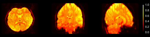
Figure C.1: Slices of the fMRI data set for one of the subjects.

The high-dimensionality of fMRI data and hence of the corresponding second order dependence structure requires an efficient method to allow for the functional eigenanalysis. To make this computationally efficient and to avoid spurious identifiability issues that come with alternative discretized matrix approaches [see 1, for a discussion], we shall assume the functional component has a separable structure. The assumption of separable functions in the context of brain imaging is commonly applied as a method to deal with the high dimensionality of this type of data [see e.g., 7, 5, 1, 6] To make this more precise in our set up, let $\prod_{i=1}^{3}\mathcal{S}_{i}$ be a product of compact sets. Then we model each fMRI data set as a functional time series $\{X_{t}(\tau_{1},\tau_{2},\tau_{3}):\tau_{i}\in\mathcal{S}_{i},i=1,2,3\}_{t\in\mathbb{Z}}$ with well-defined spectral density operator in $S_{2}(\prod_{i=1}^{3}\mathcal{S}_{i})$ that satisfies

$$\mathcal{F}^{(\omega)}_{X}=\mathcal{F}^{(\omega)}_{X,1}\widetilde{\bigotimes}\mathcal{F}^{(\omega)}_{X,2}\widetilde{\bigotimes}\mathcal{F}^{(\omega)}_{X,3},$$ (B.11)

where $\mathcal{F}^{(\omega)}_{X,i}$ denotes the $i$-th directional spectral density operator which has a kernel function in $L^{2}_{\mathbb{C}}(\mathcal{S}_{i}\times\mathcal{S}_{i})$ that replicates across the other two directions. For example, the first directional component has kernel given by

$$\mathcal{F}^{(\omega)}_{X,1}(\tau_{1},\sigma_{1})=\frac{1}{2\pi}\sum_{h\in\mathbb{Z}}\int_{\mathcal{S}_{2}}\int_{\mathcal{S}_{3}}\text{Cov}\big{(}X_{h}(\tau_{1},\tau_{2},\tau_{3}),X_{0}(\sigma_{1},\tau_{2},\tau_{3})\big{)}d\tau_{2}d\tau_{3}e^{-\mathrm{i}h\omega}\quad\tau_{1},\sigma_{1}\in\mathcal{S}_{1},$$

The kernels of $\mathcal{F}^{(\omega)}_{X,2}$ and $\mathcal{F}^{(\omega)}_{X,3}$ are similarly defined. Let the eigenelements of $\mathcal{F}^{(\omega)}_{X,i}$ be denoted as $\big{\{}\lambda^{(\omega)}_{i,j},\phi^{(\omega)}_{i,j}\big{\}}_{j\geq 1}$ for $i=1,2,3$. Then the eigendecomposition of the operator in (B.11) at frequency $\omega$ is given by

$$\mathcal{F}^{(\omega)}_{X}=\sum_{j,k,l=1}^{\infty}\lambda^{(\omega)}_{jkl}\Pi^{(\omega)}_{jkl}{\bigotimes}\Pi^{(\omega)}_{jkl}.$$ (B.12)

where the eigenvalues $\lambda^{(\omega)}_{jkl}:=\lambda^{(\omega)}_{1,j}\lambda^{(\omega)}_{2,k}\lambda^{(\omega)}_{3,l}$ are ordered in a descending manner, i.e., $\{\lambda^{(\omega)}_{jkl}\}_{jkl}\searrow 0$ and where $\Pi^{(\omega)}_{jkl}=\phi^{(\omega)}_{1,j}\otimes\phi^{(\omega)}_{2,k}\otimes\phi^{(\omega)}_{3,l}$ is the eigenfunction belonging the $jkl$-th largest eigenvalue at frequency $\omega$ (see also subsection A.2). The sequential eigenelements can now be efficiently estimated via consistent estimators of the sequential eigenelements of the directional operators as given in (3). For example, the estimator of the first directional sequential spectral density kernels is defined as

$$\hat{\mathcal{F}}_{X,1}^{(\omega)}(\eta)(\tau_{1},\sigma_{1})=\frac{1}{\lfloor\eta T\rfloor}\sum_{s=1}^{\lfloor\eta T\rfloor}\Bigg{(}\sum_{t=1}^{\lfloor\eta T\rfloor}\frac{\tilde{w}^{(\omega)}_{b,s,t}}{|\mathcal{S}_{2}||\mathcal{S}_{3}|}\sum_{\begin{subarray}{c}\tau_{2}\in\mathcal{S}_{2}\\ \tau_{3}\in\mathcal{S}_{3}\end{subarray}}(X_{s}(\tau_{1},\tau_{2},\tau_{3})(X_{t}(\sigma_{1},\tau_{2},\tau_{3})\Big{)},\quad\tau_{1},\sigma_{1}\in\mathcal{S}_{1},$$

where $|\mathcal{S}_{i}|$ is the set of the discrete observations of the function in the $i$-th direction.

The raw data was converted into functional observations by using cubic b-spline functions on $[0,1]^{3}$. It is worth mentioning that in the computation of the eigenfunctions we took into account that the B-spline basis functions do not form an orthogonal basis. Estimators of the sequential sequence of directional spectral density kernels were obtained using the same parameters as in the previous section and evaluated at a $100^{2}$ equispaced grid of $[0,1]^{2}$. We then investigated whether we could find evidence of relevant differences in the second order structure of the different subjects by applying the three tests developed in Section 3.1-3.3 pairwise. Since the sampling rate of the data is $0.5$ Hertz per second, we restrict our analysis to the interval $[0,\pi/2)$.

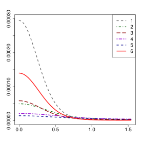
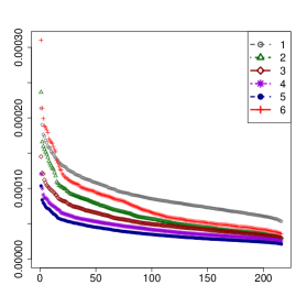
Figure C.2: Squared Hilbert-Schmidt norm of the estimator of (B.12) as a function of frequency for the 6 subjects (left) and the corresponding largest 216 eigenvalues averaged over $[0,\pi/2)$ (right).

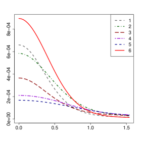
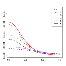
Figure C.3: The first (left) and second (right) estimated eigenvalues of (B.12) as a function of frequency for the six subjects.

In Figure (C.2), the squared Hilbert-Schmidt norm of the estimator of (B.12) is plotted as a function of frequency for each of the six subjects. We observe most signal in the low-frequency band (¡0.1 Hertz). The first 216 estimated eigenvalues averaged over frequences are given in the right graph. For fixed frequency, these were obtained by taking the first $T^{1/3}={(225)}^{1/3}$ eigenvalues of each of the directional operators, taking the kronecker product of these eigenvalues and arranging the resulting values in descending order. For all subjects, a clear gap is present after approximately 2 to 3 largest averaged eigenvalues, which then taper off slowly. Tables 1–3 provides the p-values of the test statistics $\hat{\mathbb{D}}^{[a,b]}_{T_{1},T_{2}}$, $\widehat{\mathbb{D}}^{[a,b],k}_{\Pi,T_{1},T_{2}}$ and $\widehat{\mathbb{D}}^{[a,b],k}_{\lambda,T_{1},T_{2}}$, respectively, for the specified relevant hypotheses. To clarify that the tests were conducted over the frequency band $[a,b]$, the hypotheses values are equipped with a superscript $[a,b]$, e.g., we write $\Delta^{[a,b]}$. For the testing frameworks of no relevant differences between the spectral density operator and between the eigenvalues, the thresholds $\Delta^{[a,b]}$ and $\Delta_{\lambda,i}^{[a,b]}$ are specified based upon the overall signal present in the data.

For the hypothesis of a relevant difference of at most $\Delta_{[0,\pi/2)}=1e-06$ between the spectral density operators, we observe only between subjects 3 and 5 approximately a rejection at the 6% level, but not for $\Delta_{[0,\pi/2)}=2e-06$. When we restrict to the frequency band where most signal is present (¡0.1 Hertz), we find p-values less than $0.05$ for subjects 3 and 5 and we find some marginal evidence of relevant differences for between subjects 2 and 4 with a p-value of $0.11$ for the hypothesis $\Delta_{[0,\pi/5]}=1e-06$. For the first two eigenvalues, which are plotted in Figure C.3, we do not find evidence of significant differences (Table 3), also not when we restrict to $[0,\pi/5]$ or when we change the value of $\Delta^{[0,\pi/2)}_{\lambda,i}$. This appears to be caused by a relatively large variance.

More interestingly, Table 2 provides clear evidence of relevant differences between the eigenprojectors. The null of no relevant differences between the first eigenprojectors with $\Delta^{[0,\pi/2)}_{\Pi,1}=0.2$ can be rejected for quite a few combinations at the 10% level and in particular for all those combinations with subject 1, for which the p-values are less than $0.07$. The p-values corresponding to the hypotheses $\Delta^{[0,\pi/2)}_{\Pi,1}=0.3$ provides for some pairs less clear evidence of relevant differences in the first eigenprojector. In case of the second eigenprojectors, we do however reject the null of no relevant differences for both the hypotheses $\Delta^{[0,\pi/2)}_{\Pi,2}=0.2$ and $\Delta^{[0,\pi/2)}_{\Pi,2}=0.3$ in most cases at a 1% or 5% level. Except for the tests between subject 2 and 6, we in fact reject all cases at 10% level. This behavior did not change when we restricted to $[0,\pi/5]$.

This preliminary analysis would indicate that differences in brain activity between subjects might be driven by differences in shapes in their primary modes of variation. However, given the complexity of the data a more detailed analysis and a longer observation length might be of interest. This is however beyond the scope of this paper and is left for future research.

$H_{0}:\Delta^{[0,\pi/2)}=1e-06$
	2	3	4	5	6
1	0.336	0.328	0.296	0.269	0.422
2		0.375	0.193	0.175	0.227
3			0.175	0.053	0.176
4				0.957	0.19
5					0.185

$H_{0}:\Delta^{[0,\pi/2)}=2e-06$
2	3	4	5	6
0.341	0.337	0.299	0.272	0.434
	0.829	0.496	0.287	0.265
		0.364	0.141	0.218
			0.998	0.208
				0.204

$H_{0}:\Delta^{[0,\frac{\pi}{5}]}=1e-06$
	2	3	4	5	6
1	0.332	0.326	0.296	0.265	0.416
2		0.242	0.107	0.127	0.214
3			0.129	0.031	0.15
4				0.615	0.187
5					0.182

$H_{0}:\Delta^{[0,\frac{\pi}{5}]}=2e-06$
2	3	4	5	6
0.337	0.328	0.296	0.27	0.422
	0.403	0.182	0.167	0.234
		0.196	0.046	0.177
			0.946	0.2
				0.189

Table 1: $p$-values corresponding to the test in Theorem 3.3 for the specified null hypotheses and frequency bands.

$H_{0}:\Delta^{[0,\pi/2)}_{\Pi,1}=0.2$
	2	3	4	5	6
1	0.001	0.001	0.061	0.014	0.064
2		0.073	0.314	0.289	0.465
3			0.043	0.122	0.131
4				0.583	0.375
5					0.278

$H_{0}:\Delta^{[0,\pi/2)}_{\Pi,2}=0.2$
2	3	4	5	6
0.004	0.031	0.057	0.034	0.024
	0.006	0.001	0.007	0.195
		0.004	0.007	0.029
			0.019	0.004
				0.056

$H_{0}:\Delta^{[0,\pi/2)}_{\Pi,1}=0.3$
	2	3	4	5	6
1	0.002	0.001	0.132	0.036	0.17
2		0.205	0.482	0.414	0.627
3			0.117	0.282	0.242
4				0.887	0.508
5					0.42

$H_{0}:\Delta^{[0,\pi/2)}_{\Pi,2}=0.3$
2	3	4	5	6
0.007	0.038	0.076	0.043	0.038
	0.014	0.001	0.016	0.24
		0.007	0.016	0.039
			0.039	0.007
				0.08

Table 2: $p$-values corresponding to the eigenprojector test (Theorem 3.5) applied to the first two eigenprojectors for the stated hypotheses.

$H_{0}:\Delta^{[0,\pi/2]}_{\lambda,1}=(2e-06)^{2}$
	2	3	4	5	6
1	0.473	0.342	0.311	0.264	0.341
2		0.289	0.239	0.234	0.214
3			0.304	0.184	0.241
4				0.291	0.215
5					0.216

$H_{0}:\Delta^{[0,\pi/2]}_{\lambda,2}=(2e-06)^{2}$
2	3	4	5	6
0.446	0.32	0.302	0.255	0.487
	0.295	0.204	0.206	0.204
		0.319	0.2	0.207
			0.255	0.187
				0.196

Table 3: $p$-values corresponding to the eigenvalue test (Theorem 3.7) applied to the first two eigenvalues for the stated hypotheses.

References

- Antoniadis et al. [2006] Antoniadis, A., Paparoditis, E. and Sapatinas, T. (2006). A functional wavelet-kernel approach for time series prediction. Journal of the Royal Statistical Society: Series B (Statistical Methodology), 68:837–857.
- Aston and Kirch [2012] Aston, J. A. and Kirch, C. (2012). Detecting and estimating changes in dependent functional data. Journal of Multivariate Analysis, 109:204–220.
- Aue et al. [2019] Aue, A., Dette, H., and Rice, G. (2019). Two-sample tests for relevant differences in the eigenfunctions of covariance operators. arXiv:1909.06098.
- Benko et al. [2009] Benko, M., Härdle, W., and Kneip, A. (2009). Common functional principal components. Annals of Statistics, 37:1–34.
- [5] Joseph Berkson. Some difficulties of interpretation encountered in the application of the chi-square test. Journal of the American Statistical Association, 33:526–536, 1938.
- van Delft [2020] van Delft, A. (2020). A note on quadratic forms of functional time series under mild conditions. Stochastic Processes and their Applications, 130(7):4206–4251.
- van Delft and Eichler [2020] van Delft, A. & Eichler, M (2020). A note on Herglotz’s theorem for time series on function spaces. Stochastic Processes and their Applications, 130(6):3687–3710.
- van Delft and Dette [2020] van Delft, A. & Dette, H. (2020). A similarity measure for second order properties of non-stationary functional time series with applications to clustering and testing. Bernoulli, to appear.
- van Delft and Dette [2020] van Delft, A. & Dette, H. (2020). Supplement to “Pivotal tests for relevant differences in the second order dynamics of functional time series”.
- van Delft and Eichler [2018] van Delft, A. & Eichler, M. “Locally stationary functional time series.” Electronic Journal of Statistics, 12:107–170 (2018).
- Deheuvels and Martynov [2003] Deheuvels, P. and Martynov, G. (2003). Karhunen-Loève expansions for weighted Wiener processes and Brownian bridges via Bessel functions. High dimensional probability, III (Sandjberg, 2002). Progr. Probab. 55 57–93. Birkhauser, Basel.
- Dette et al. [2020] Dette, H., Kokot, K., and Volgushev, S. (2020). Testing relevant hypotheses in functional time series via self-normalization. To appear in: Journal of the Royal Statistical Society: Series B arXiv:1809.06092.
- Fiecas and Ombao [2016] Fiecas, M., and Ombao, H. (2016). Modeling the Evolution of Dynamic Brain Processes during an Associative Learning Experiment. Journal of the American Statistical Association, 111:1440–1453.
- Fremdt et al. [2013] Fremdt, S., Steinebach, J. G., Horváth, L., and Kokoszka, P. (2013). Testing the equality of covariance operators in functional samples. Scandinavian Journal of Statistics, 40(1):138–152.
- Fogarty & Small [2014] Fogarty, C. B. & Small, D. S. (2014). Equivalence testing for functional data with an application to comparing pulmonary function devices. Ann. Appl. Stat. 8, 2002–2026.
- Guo et al., [2016] Guo, J., Zhou, B., and Zhang, J.-T. (2016). A supremum-norm based test for the equality of several covariance functions. Computational Statistics & Data Analysis, 124:15–26.
- Hörmann and Kokoszka [2010] Hörmann, S. & Kokoszka, P. (2010). Weakly dependent functional data. The Annals of Statistics, 38:1845–1884.
- Hörmann et al. [2015] Hörmann S., Kidziński, L. & Hallin, M. (2015). Dynamic functional principal components. The Royal Statistical Society: Series B 77:319–348.
- Hörmann et al. [2018] Hörmann, S., Kokoszka, P. & Nisol, G. (2018). Detection of periodicity in functional time series. The Annals of Statistics. 46:2960–2984.
- Kadison and Ringrose [1997] Kadison, R.V. & Ringrose, J. R. (1997). Fundamentals of the Theory of Operator Algebras. Graduate Studies in Mathematics. Amer. Math. Soc., Providence, RI.
- Kowal et al. [2019] Kowal, D.R., Matteson, D.S. and Ruppert, D. (2019). Functional autoregression for sparsely sampled data. Journal of Business and Economics Statistics 37:97–109.
- Leucht et al. [2018] Leucht, A., Paporoditis, E. and Sapatinas, T. (2018). Testing equality of spectral density operators for functional linear processes. arXiv:1804.03366.
- McLeish [1974] McLeish, D. L. (1974). Dependent central limit theorems and invariance principles. The Annals of Probability, 2:620–628.
- Mòricz [1976] Mòricz, F. (1976). Moment inequalities and the strong law of large numbers. Z. Wahrscheinlichkeitstheorie verw. Gebiete , 35:299–314.
- Panaretos et al. [2010] Panaretos, V. M., Kraus, D., and Maddocks, J. H. (2010). Second-order comparison of gaussian random functions and the geometry of dna minicircles. Journal of the American Statistical Association, 105(490):670–682.
- Panaretos and Tavakoli [2013] Panaretos, V. and Tavakoli, S. (2013). Cramér–Karhunen–Loève representation and harmonic principal component analysis of functional time series. Stochastic Processes and their Applications 123:2779–2807.
- Panaretos and Tavakoli [2013a] Panaretos, V. and Tavakoli, S. (2013a). Fourier analysis of stationary time series in function space. The Annals of Statistics 41(2):568–603.
- Paparoditis and Sapatinas [2016] Paparoditis, E. and Sapatinas, T. (2016). Bootstrap-based testing of equality of mean functions or equality of covariance operators for functional data. Biometrika, 103(3):727–733.
- Pilavakis et al. [2019] Pilavakis, D., Paparoditis, E., and Sapatinas, T. (2019). Testing equality of autocovariance operators for functional time series. ArXiv e-print 1901.08535.
- Pomann et al. [2016] Pomann, G.-M., Staicu, A.-M., and Ghosh, S. (2016) A two-sample distribution-free test for functional data with application to a diffusion tensor imaging study of multiple sclerosis. Journal of the Royal Statistical Society, Series C, 65:395–414.
- Shao [2010] Shao, X. (2010). A self-normalized approach to confidence interval construction in time series. Journal of the Royal Statistical Society: Series B (Statistical Methodology), 72(3):343–366.
- Shao [2015] Shao, X. (2015). Self-normalization for time series: A review of recent developments. Journal of the American Statistical Association, 110(512):1797–1817.
- Shao and Zhang [2010] Shao, X. and Zhang, X. (2010). Testing for change points in time series. Journal of the American Statistical Association, 105(491):1228–1240.
- Tavakoli and Panaretos [2016] Tavakoli, S. and Panaretos, V. (2016) Detecting and Localizing Differences in Functional Time Series Dynamics: A Case Study in Molecular Biophysics Journal of the American Statistical Association, 111:1020–1035.
- [35] Stefan Wellek. Testing Statistical Hypotheses of Equivalence and Noninferiority. CRC Press, Boca Raton, FL, second edition, 2010.
- Wu [2005] Wu, W. B. (2005). Nonlinear system theory: Another look at dependence. Proceedings of the National Academy of Sciences., 102:14150–14154.
- Yuen et al. [2019] Yuen N.H., Osachoff N., and Chen J.J. (2019). Intrinsic Frequencies of the Resting-State fMRI Signal: The Frequency Dependence of Functional Connectivity and the Effect of Mode Mixing. Frontiers in Neuroscience, 13:900–917.
- Zhang and Shao [2015] Zhang, X. and Shao, X. (2015). Two sample inference for the second-order property of temporally dependent functional data. Bernoulli 21:90–929.
- Zhang et al. [2011] Zhang, X., Shao, X., Hayhoe, K., and Wuebbles, D. J. (2011). Testing the structural stability of temporally dependent functional observations and application to climate projections. Electron. J. Statist., 5:1765–1796.

References

- Aston and Kirch [2012] Aston, J. A. and Kirch, C. (2012). Detecting and estimating changes in dependent functional data. Journal of Multivariate Analysis, 109:204–220.
- Biswal et al. [2010] Biswal, B.B. et al. (2010). Toward discovery science of human brain function. Proc. Natl. Acad. Sci. USA, 107:4734–4739.
- van Delft [2020] van Delft, A. (2020). A note on quadratic forms of functional time series under mild conditions. Stochastic Processes and their Applications, 130(7):4206–4251. arXiv:1905.13186.
- McLeish [1974] McLeish, D. L. (1974). Dependent central limit theorems and invariance principles. The Annals of Probability, 2:620–628.
- Ruttimann et al. [1998] Ruttimann, U.E. et al. (1998). Statistical analysis of functional MRI data in the wavelet domain. IEEE Transactions on Medical Imaging, 17(2):142–154.
- Stoehr et al. [2019] Stoehr, C., Aston, J. A. and Kirch, C. (2019). Detecting changes in the covariance structure of functional time series with application to fMRI data. arXiv:1903.00288.
- Worsley et al. [2002] Worsley, K.J, Liao, C.H., Aston, J., Petre, V., Duncan, G.H., Morales, F. and Evans, A.C. (2015). A general statistical analysis for fMRI data. Neuroimage 15:1–15.
- Mòricz [1976] Mòricz, F. (1976). Moment inequalities and the strong law of large numbers. Z. Wahrscheinlichkeitstheorie verw. Gebiete , 35:299–314.