Giant ratchet magneto-photocurrent in graphene lateral superlattices
Abstract
We report on the observation of the magnetic quantum ratchet effect in graphene with a lateral dual-grating top gate (DGG) superlattice. We show that the THz ratchet current exhibits sign-alternating magneto-oscillations due to the Shubnikov-de Haas effect. The amplitude of these oscillations is greatly enhanced as compared to the ratchet effect at zero magnetic field. The direction of the current is determined by the lateral asymmetry which can be controlled by variation of gate potentials in DGG. We also study the dependence of the ratchet current on the orientation of the terahertz electric field (for linear polarization) and on the radiation helicity (for circular polarization). Notably, in the latter case, switching from right- to left-circularly polarized radiation results in an inversion of the photocurrent direction. We demonstrate that most of our observations can be well fitted by the drift-diffusion approximation based on the Boltzmann kinetic equation with the Landau quantization fully encoded in the oscillations of the density of states.
I Introduction
The discovery of graphene opened a new research direction in condensed matter physics. The unique optical properties of this material prompted a rapid development of photonics and optoelectronics, see, e.g., Refs. Castro Neto et al. (2009); Bonaccorso et al. (2010); Mueller et al. (2010); Echtermeyer et al. (2011); Novoselov et al. (2012); Grigorenko et al. (2012). These are especially important for applications in the terahertz (THz) range of frequencies, see THz roadmap Dhillon et al. (2017) and Graham et al. (2012); Mittendorff et al. (2013); Freitag et al. (2013); Ryzhii et al. (2014); Cai et al. (2014); Mittendorff et al. (2015); Otsuji et al. (2012); Koseki et al. (2016); Bandurin et al. (2018a); Vicarelli et al. (2012); Hartmann et al. (2014); Tredicucci and Vitiello (2014). THz-radiation-induced non-linear optical effects, including rectification of THz/infrared electromagnetic waves, offer a new playground for many intriguing phenomena in graphene, see, e.g., reviews Otsuji et al. (2012); Glazov and Ganichev (2014); Koppens et al. (2014); Low and Avouris (2014); Hasan et al. (2016); Ganichev et al. (2018); You et al. (2018); Rogalski et al. (2019); Wang et al. (2019). These phenomena deliver graphene-specific mechanisms of photocurrent generation and provide a basis for the development of novel graphene radiation plasmonic detectors. Such detectors are compact, tunable by gate voltage and have already shown fast and sensitive operation in a broad frequency band from sub-THz to infrared, and from ambient- to cryogenic temperatures Mittendorff et al. (2013); Freitag et al. (2013); Ryzhii et al. (2014); Cai et al. (2014); Mittendorff et al. (2015); Otsuji et al. (2012); Koseki et al. (2016); Bandurin et al. (2018a); Vicarelli et al. (2012); Hartmann et al. (2014); Tredicucci and Vitiello (2014).
Among the highly promising radiation detecting mechanisms is the ratchet effect, i.e., the generation of a electric current responding to an electric field in systems with broken -symmetry. This is one of the most general and fundamental nonlinear phenomena in optoelectronics, for reviews see, e.g., Hänggi and Marchesoni (2009); Linke (2002); Reimann (2002); Ivchenko and Ganichev (2011); Denisov et al. (2014); Bercioux and Lucignano (2015); Reichhardt and Reichhardt (2017); Ganichev et al. (2018). In graphene, the ratchet effect can be obtained in monolayers with asymmetric micro-patterns Kiselev and Golub (2011); Ermann and Shepelyansky (2011); Koniakhin (2014), layers with built-in structure inversion asymmetry (SIA) Glazov and Ganichev (2014); Jiang et al. (2011) (in this case it is typically called photogalvanic effect Ivchenko and Ganichev (2011); Weber et al. (2008a)), short-channel devices, like field effect transistors (FETs) with asymmetric boundary conditions Vicarelli et al. (2012); Tomadin et al. (2013); Muraviev et al. (2013); Spirito et al. (2014); Cai et al. (2015); Wang et al. (2015); Auton et al. (2017); Bandurin et al. (2018b, a), as well as in structures with asymmetric grating type of electrodes Ganichev et al. (2018); Nalitov et al. (2012); Otsuji et al. (2013); Rozhansky et al. (2015); Olbrich et al. (2016); Popov (2016); Fateev et al. (2017, 2019). Besides their fundamental significance, the two latter types of ratchets are extremely important for applications, since they provide a very promising route towards fast, sensitive, and gate-tunable detection of THz radiation at room temperature. The study of ratchet effects in graphene under different transport regimes such as the drift-diffusion Nalitov et al. (2012); Olbrich et al. (2016) or the hydrodynamic one Rozhansky et al. (2015); Popov (2016); Fateev et al. (2017, 2019), including plasmonic effects, is a very challenging task that has just begun to be explored.
For ratchets new physics comes into play, when an external magnetic field is applied. In recent work we showed, e.g., that a ratchet effect can be induced by an external magnetic field even in case of homogeneous graphene with structure inversion asymmetry Drexler et al. (2013). The effect was called magnetic quantum ratchet effect and belongs to the class of magneto-photogalvanic effects Fal’ko (1989); Ivchenko et al. (1988); Bel’kov et al. (2005); Tarasenko (2008); Weber et al. (2008b); Tarasenko (2011); Zoth et al. (2014). It is sensitive to disorder and tunable by a gate voltage Drexler et al. (2013). The observation triggered numerous theoretical proposals aimed to enhance and control magnetic ratchet effects in graphene-based systems. In particular, it was predicted that the magnetic ratchet effect can be enormously increased under cyclotron resonance condition and in periodic grating gate structures.
Here we report the observation of the giant oscillating magnetic ratchet effect in graphene with superimposed lateral superlattice, consisting of a dual-grating top gate (DGG) structure. We show particularly, that, the THz-radiation-induced ratchet current exhibits sign-alternating magneto-oscillations stemming from Landau quantization and having the same period as the Shubnikov-de Haas (SdH) oscillations. The amplitude of the ratchet current oscillations is greatly enhanced (at least by one order of magnitude) as compared to the ratchet effect at zero magnetic field previously studied in similar structures Olbrich et al. (2016). The latter effect was shown to be caused by the combined action of a spatially periodic in-plane potential and the spatially modulated light due to the near-field effects of the radiation diffraction Olbrich et al. (2016). Quantum oscillations appear also as a function of top/back gate voltage in our DGG structures when subjected to a constant magnetic field. Thereby, the direction of the current is controlled by the lateral asymmetry parameter Ivchenko and Ganichev (2011); Olbrich et al. (2016)
| (1) |
Here, the overline stands for the average over the ratchet period, is the derivative of the coordinate dependent electrostatic potential , and the distribution of the radiation electric field being coordinate dependent due to the near-field of diffraction. We show that by changing the individual gate voltages of the dual-grating gate structure we can controllably change the sign of and, thus, the direction of the ratchet current. Furthermore, we study the response to both linear and circularly-polarized radiation and demonstrate that the magnetic ratchet current is sensitive to the orientation of the linear polarization with respect to the fingers of the DGG structure as well as to the radiation helicity in the case of circular polarization. In the latter case switching from right- to left-circular polarization results in a phase shift of the oscillations by , i.e., at constant magnetic field, the current direction reverses. The theoretical modeling of our results is based on the experimental values of all involved parameters and the assumption that the frequency of the incoming radiation is much higher than the plasmonic frequency, so that plasmonic effects do not contribute substantially. We demonstrate that in strong quantizing magnetic fields all observations can be well fitted by the drift-diffusion approximation of the kinetic Boltzmann equation. Within this approach we find that the photocurrent is proportional to second derivative of the longitudinal resistance and, therefore, almost follows the Shubnikov-de Haas resistance oscillations with a large enhancement factor arising due to differentiating of rapidly oscillating function.
The paper is organized as follows. In Sec. II we describe the investigated samples and experimental technique. In Sec. III we discuss the observed magnetic ratchet effects generated by linearly and circularly polarized THz radiation. In the following Secs. IV and V we present the theory and compare the corresponding results with the experimental data. Finally, in Sec. VI we summarize the results.
II Samples and methods
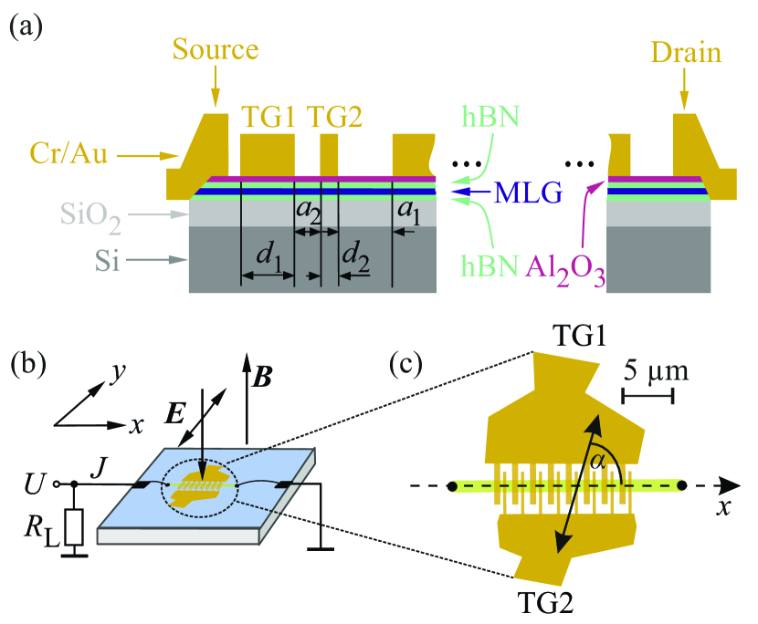
Single-layer graphene samples encapsulated in hexagonal boron nitride (\cehBN) were prepared using the van-der-Waals stacking technique with Cr/Au edge contacts established by Wang et al. Wang et al. (2013). After exfoliation and stacking on top of a silicon wafer with thermal oxide, a Hall bar mesa was etched using \ceCHF_3 based reactive ion etching, and edge contacts were deposited by thermal evaporation. To avoid gate leakage at the mesa sidewalls, the samples were covered with \ceAl_2O_3 using atomic layer deposition. The highly doped Si wafer serves as a uniform back gate.
Afterwards, following the recipe of Ref. Olbrich et al. (2016), a dual-grating top gate (DGG) superlattice was fabricated on top of the hBN/graphene/hBN flakes for the measurement of the ratchet photocurrent. The micropatterned periodic DGG fingers were made by electron beam lithography and subsequent deposition of metal ( Cr and Au) on graphene covered by hBN and a \ceAl_2O_3 layer. A sketch of this superstructure is shown in Figs. 1(a) and 1(c). Two gate stripes with different widths and and spacings and in between form the supercell of the lattice. The cell is repeated eight times resulting in a superlattice with a total length of . All wide stripes were connected forming multifinger top gate electrode TG1. Similarly connected narrow stripes formed gate electrode TG2, see yellow areas in Fig. 1(c). Independent bias voltages (, ) could be applied to wide and narrow gate stripes making the electrostatic potential asymmetry in the graphene tunable. The width of the whole structure is yielding the total area .
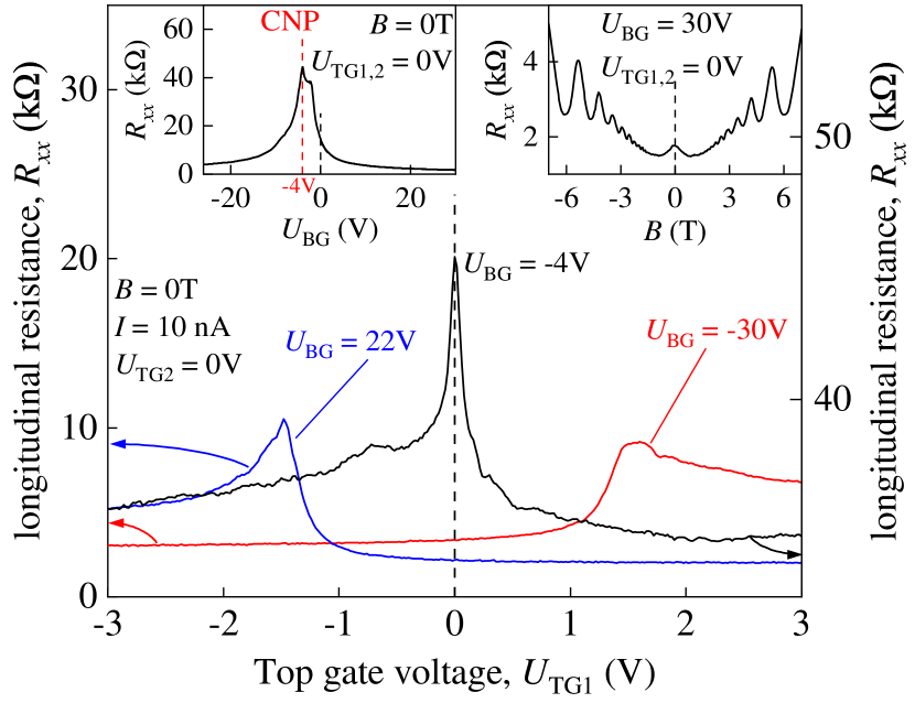
To measure the longitudinal resistance and the photocurrent normal to the DGG stripes Ohmic contacts were fabricated, see Fig. 1(c). Low temperature transport measurements, which are possible in our structure in two-point configuration only, showed well resolved SdH oscillations, see right inset in Fig. 2. The oscillatory part was obtained by subtracting a polynomial background of the form from the longitudinal resistance . The coefficients , and were obtained by fitting to the high field data. Also a clear charge neutrality point was observed at while tuning the Fermi energy by sweeping the back gate, see left inset of Fig. 2. We obtained an electron mobility and a hole mobility of at . Application of a positive top gate potential shifts the peak of the longitudinal resistance to higher negative while for high negative top gate voltages it moves to positive , see Fig. 2.
As a radiation source for our experiments a continuous wave methanol terahertz laser with a radiation frequency of () and a radiation power of the order of was used Kvon et al. (2008); Ganichev et al. (2009); Olbrich et al. (2013). The radiation was focused onto the sample using an off-axis parabolic mirror resulting in a spot size of , which yields an intensity . The radiation power coming onto the sample is calculated after . The laser beam had an gaussian shape as checked by a pyroelectric camera Ganichev (1999); Ziemann et al. (2000). The radiation was modulated at about by an optical chopper in order to use standard lock-in technique.
The optically pumped molecular laser used here emits linearly polarized radiation. In our setup its polarization plane is oriented along the -axis being normal to the dual-grating gate stripes. In experiments with linearly polarized radiation, the orientation of the radiation electric field vector was varied by rotation of a mesh grid polarizer mounted behind the quarter-wave plate providing circularly polarized radiation. The azimuth angle is the angle between the radiation electric field vector and the -direction, Fig. 1(c). The Stokes parameters describe the degree of the linear polarization in the basis (, ) and the basis (, ) rotated by and , respectively. In this setup, they are given by
| (2) |
In experiments with elliptically polarized radiation, the radiation helicity was varied by rotating the quarter-wave plate by the angle . By that, at = 0 radiation is linearly polarized and is parallel to , whereas at and the radiation is circularly polarized with opposite helicities. In this setup the Stokes parameters are given by Bel’kov et al. (2005); Weber et al. (2008a)
| (3) | |||||
where defines the degree of circular polarization. The ratchet photocurrents were measured in a magneto-optical cryostat at a temperature of as a voltage drop along a load resistor of using standard lock-in technique and then calculated using . In all graphs, the photocurrent is normalized to the radiation power coming onto the sample, . An external magnetic field with up to is applied normal to the graphene plane, as sketched in Fig. 1(b).

III Results
Before discussing our results on magnetic current we briefly address the photocurrents detected at zero magnetic field. In our previous work Olbrich et al. (2016), in which we studied similar structures and applying terahertz radiation with the same parameters, we demonstrated that illumination of the DGG superlattice on graphene results in a photocurrent exhibiting characteristic behavior of the ratchet effect. In particular, photocurrent direction and magnitude: (i) are sensitive to the orientation of the radiation electric field vector and/or the radiation helicity; (ii) depend on the carrier charge sign (electrons/holes); (iii) are controlled by the lateral asymmetry parameter , which can be varied by applying voltages and to the individual subgates. Note that, switching of the gate voltage from , to , leads to a change in the sign of and, as a consequence, to a reversal of the photocurrent direction. Theoretical analysis carried out in Ref. Olbrich et al. (2016) reveals that the photocurrent is caused by a combined action of a spatially periodic in-plane electrostatic potential and the radiation spatially modulated due to the near-field effects of the diffraction on the DGG stripes. Experiments and theory of this effect present a self-consisted detailed picture of the ratchet current formation, therefore, in the present paper we focused on the magnetic ratchet effect in graphene.
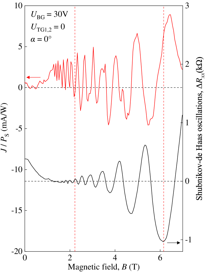
Applying an external magnetic field we observed that the ratchet photocurrent drastically changes: The photocurrent exhibits sign-alternating SdH-like magneto-oscillations with an amplitude by more than an order of magnitude larger than the photocurrent at zero magnetic field. A characteristic magnetic field dependence is shown in Fig. 3 for , radiation electric field oriented perpendicular to the gate stripes and back gate voltage = . Note that at zero top gate voltages, the lateral asymmetry is created by the built-in potential caused by the metal stripes deposited on top of graphene.
Comparing the magnetic-field dependencies of the ratchet photocurrent and the longitudinal resistance we found out that extrema positions of the photocurrent and the SdH oscillations coincide in weak fields. This is seen clearly in Fig. 3, where the left vertical dashed line exemplary indicates extrema positions of the photocurrent and the SdH oscillations. It should be noted that, whereas at low magnetic fields the photocurrent oscillations follow , at high magnetic fields a magnetic field-dependent phase shift is present, see right vertical dashed line in Fig. 3. These fields are slightly higher than the magnetic field of the cyclotron resonance , where , , and are the radiation angular frequency , Fermi energy, and the Dirac velocity in graphene, respectively. Note that for the carrier density , and radiation frequency , relevant to experiment, we estimated .
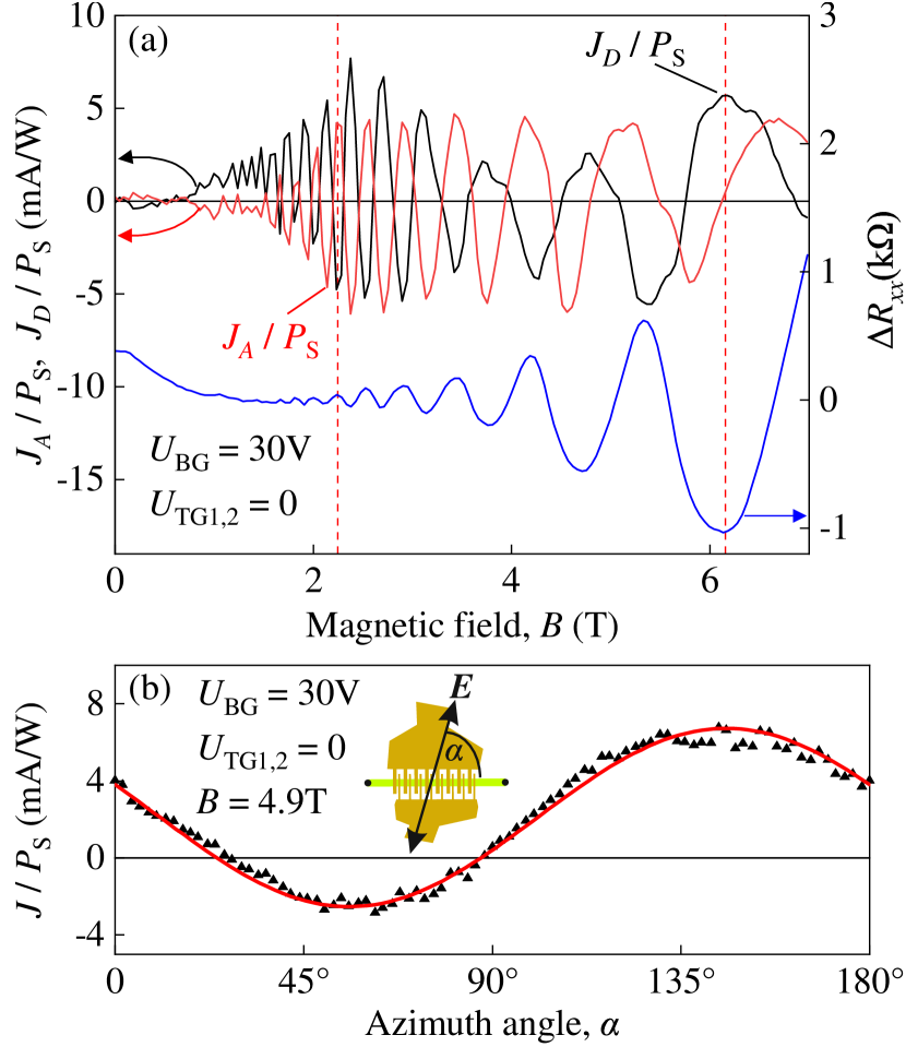
The resistance oscillations can also be obtained at fixed magnetic field by the variation of the carrier density , e.g. changing the back gate voltage (). This kind of oscillations we also observed in the ratchet photocurrent. Figure 4 shows an example of such oscillations obtained for , , and for linear polarization with .
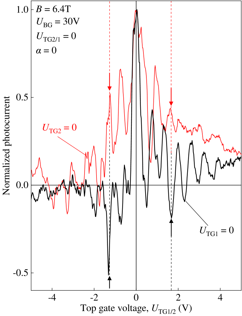
Now we turn to the results obtained by variation of the lateral asymmetry applying different voltages to the top subgates TG1 and TG2. Figure 5 shows magnetic ratchet photocurrent oscillations as a function of top gate voltage () obtained for zero biased top gate TG2 (TG1), and for linear polarization with . At zero top gate voltages the photocurrent has the same sign and almost the same amplitude. Sweeping voltage of one of the top gates while holding the other one at zero bias we observed that the photocurrent oscillates in a similar way as it is detected for the variation of back gate voltage. However, the period of oscillations is substantially decreased, which clearly follows from the different separation between top/back gates and graphene. At high gate voltages corresponding to stronger lateral asymmetry as the built-in one we observed that maxima (minima) of the dependence on corresponds to minima (maxima) of the dependence on . This is illustrated in Fig. 5 for positive and negative top gate voltages by vertical red/black dashed lines. It reveals that the change of sign of the lateral asymmetry parameter results in the change of the oscillations sign, as expected for the ratchet effect. Indeed, e.g., for the top gate voltage combinations marked by the right vertical dashed lines (, , red curve, and , , black curve) the signs of the asymmetry parameters are opposite.
All results discussed previously were obtained for linearly polarized radiation with the electric field perpendicular to the DGG stripes. Further experiments demonstrate that magneto-oscillations of the ratchet current are sensitive to the orientation of the THz electric field vector, see Fig. 6. Our measurements demonstrate that dependence of the current on the direction of the linear polarization can be well fitted as follows
| (4) |
where , , and are magnetic field-dependent fitting parameters. Figure 6(b) exemplary shows the polarization dependence of the total photocurrent measured at fixed magnetic field . The magnetic field dependence of the coefficients and yielding dominating contributions at low magnetic field are presented in Fig. 6(a). The curves in Fig. 6(a) were obtained from the magnetic field dependence of the photocurrent excited by the THz electric field vectors oriented perpendicular () and parallel () to the stripes. For these angles the photocurrent contribution is zero and the total current is given by . Consequently, the magnetic field dependencies of and were calculated, respectively, as a half-difference and half-sum of the photocurrents measured for and . Figure 6(a) reveals that these ratchet current contributions have opposite signs and close magnitudes.
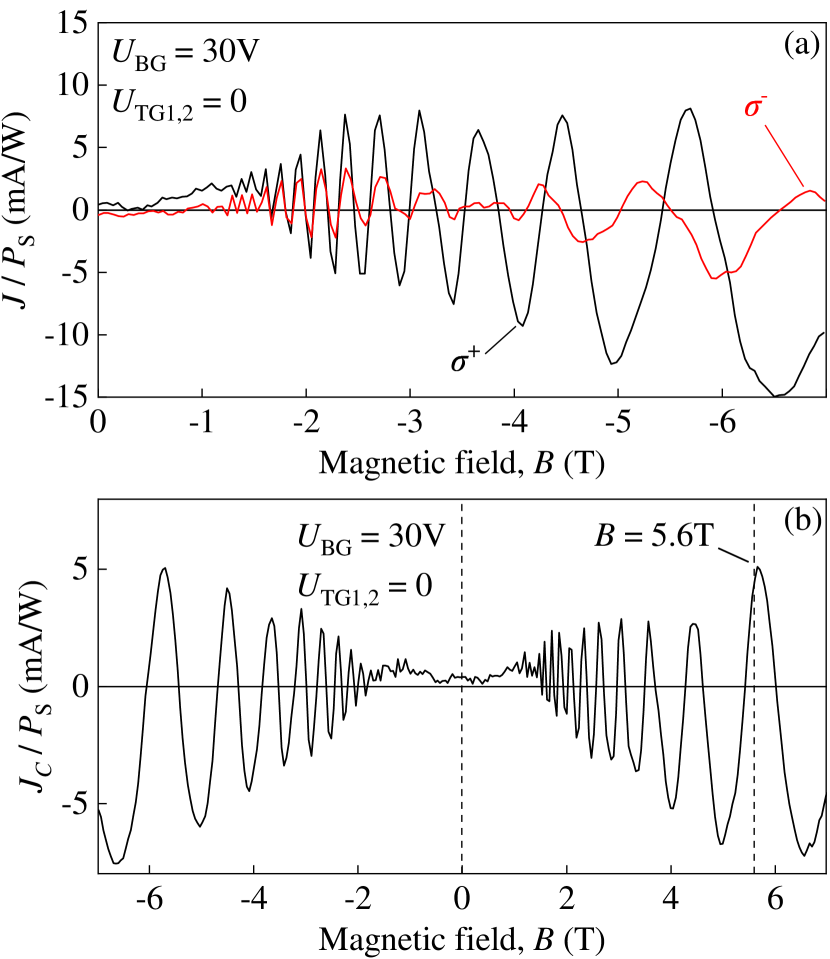
Above we discussed experiments with linear polarization rotated by plate. Let us now discuss experimental data obtained by using plate which allows us to create circular polarization. Figure 7(a) shows magneto-oscillations of the photocurrent excited by right- () and left-handed () circularly polarized radiation. Subtracting these two curves we obtain the amplitude of the helicity-sensitive photocurrent given by
| (5) |
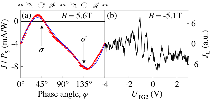
This treatment extracts the photocurrent contribution whose direction reverses upon switching the radiation helicity. Note that for circularly polarized radiation the degrees of linear polarization and are equal to zero and, consequently, the magnetic ratchet effect caused by the linearly polarized radiation vanishes. This sign-reversion has been observed directly by measuring the dependence of the photocurrent on the phase angle defining the radiation helicity after Eq. (3). This is shown in Fig. 8(a), where the helicity dependence of the ratchet photocurrent is studied at , corresponding to the maximum of , see Fig. 7(b). The overall polarization dependence of the photocurrent can be well fitted by
| (6) |
where , , , and are magnetic field-dependent fitting parameters. Figure 8(a) demonstrates that the circular photocurrent yields substantial contribution to the total photocurrent. Similar to the linear ratchet effect the circular photocurrent shows clear oscillations upon variation of the gate potential, see Fig. 8(b) for .
To summarize the experimental results, we observed that excitation of the DGG superlattice with THz radiation results in the ratchet photocurrent showing magneto-oscillations as well as oscillations upon variation of back/top gate voltages. The oscillations are closely related to the Shubnikov-de Haas effect. Measurements with controllable variation of the top gate voltages and, correspondingly, the lateral asymmetry parameter clearly demonstrate that the photocurrent is caused by the ratchet effect. The photocurrent is giantly enhanced in the presence of magnetic field. The experimental results show a substantial contribution of both, linear and circular magnetic ratchet effects exhibiting sign-alternating magneto-oscillations.
IV Theory
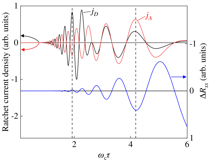
In this section we generalize the theory of magnetic ratchets to graphene-based systems in the Shubnikov-de-Haas regime. While for ratchets based on 2D systems with a parabolic energy spectrum the theory of magneto-oscillations was developed in Refs. Budkin et al. (2016); Faltermeier et al. (2017, 2018) it can not be applied to graphene. Moreover, as it has been demonstrated in Ref. Nalitov et al. (2012), even at zero magnetic field the ratchet currents are drastically different in systems with linear and parabolic energy dispersions.
We use the Boltzmann kinetic equation approach, where the electric current density is given by the following expression
| (7) |
Here is the velocity of carriers having the momentum with being the Dirac fermion velocity, enumerates spin and valley-degenerate states, and is the distribution function averaged over the space period of DGG structure. The latter is a solution of the kinetic equation Budkin et al. (2016)
| (8) |
Here is the elastic scattering collision integral, and the space- and time-dependent force is given by
| (9) |
where is the radiation near-field acting on 2D carriers, is the radiation frequency, and is the periodic potential of the ratchet. The distribution function is found by sequential iterations of the kinetic equation in small electric field amplitude and the ratchet potential with the result linear in and quadratic in with the ratchet current proportional to the asymmetry parameter given by Eq. (1).
For zero magnetic field the polarization-dependent ratchet current density in graphene is given by Nalitov et al. (2012); Olbrich et al. (2016)
| (10) | |||
where is given by:
| (11) |
and is the electron elastic scattering time assumed to be independent of the Fermi energy.
Here we calculate the ratchet current in graphene in the Shubnikov-de-Haas regime. The quantization of the energy spectrum in strong magnetic fields is taken into account by the oscillating density of states at the Fermi energy: , where is the zero-field density of states with account for spin and valley degeneracies, and the oscillating part is given by Zoth et al. (2014); Briskot et al. (2013)
| (12) |
Here the cyclotron frequency in graphene is , and is the quantum lifetime. As a result of the density-of-states oscillations, the electron scattering rate also has an oscillating part: .
In Appendix A, we find the distribution function . Note that not only the angular-independent part of the distribution function but also its second angular harmonics contribute to the current Eq. (7) in graphene due to non-parabolicity of the Dirac fermion dispersion Nalitov et al. (2012). Averaging the product over directions of and then, integrating by the electron energy, taking into account the oscillations of the density of states, we obtain the ratchet current components in the form given in Appendix A, Eq. (58). In general, we obtain that the leading contribution to the magnetic ratchet current is proportional to . This yields 1/-oscillations which are in phase with the SdH oscillations. Note that there is also a contribution proportional to the first derivative of with respect to () phase-shifted by from . However, this contribution is small with respect to the quantum parameter , and, consequently, we omit it in the following calculations.
The obtained expressions, valid for arbitrary relation between the parameters , , and , are cumbersome, therefore we give them here in two limits of low and high magnetic fields where is much higher and much smaller than , respectively.
At (i.e. ) we have:
| (13) | ||||
| (14) | ||||
In the opposite limit () we get:
| (15) | ||||
| (16) | ||||
Here is the zero-field value of the ratchet current, Eq. (11).
Above we developed the drift-diffusion theory assuming that the impurity scattering dominates over the electron-electron scattering. The discussion of the hydrodynamic regime, where electron-electron collisions are very fast, will be presented elsewhere (previous studies on the hydrodynamic ratchet effect Rozhansky et al. (2015); Popov (2016); Fateev et al. (2017, 2019) did not discuss magneto-oscillations). Our preliminary estimates show that similar results can be obtained. In particular, we find that in the high-field limit at the ratio in accordance with Eqs. (15), (16).
V Discussion
Now we discuss the experimental results in the view of the developed theory. In the experiments, we probed the photocurrent flowing in the direction normal to the DGG stripes, because of the device geometry. The photocurrent obtained in Sec. IV is proportional to , i.e., exhibits -periodic oscillations following SdH-oscillations. Analyzing the extrema positions of the photocurrent, see Fig. 3, we obtained that the oscillations indeed correspond to the SdH oscillations of , i.e. ratchet photocurrent is proportional to as expected from Eqs. (13), (15). We note that at high magnetic fields the experimentally observed ratchet current oscillations have a magnetic field dependent phase shift, and, hence, the photocurrent is phase-shifted in respect to the oscillations of . Exploring this exciting feature requires additional experimental and theoretical studies, and is out of scope of this paper.
From Eqs. (13) and (15) together with Eq. (12) we expect sign-alternating oscillations of the magnetic ratchet current as a function of Fermi energy and, consequently, gate voltages. The oscillations periodic in gate voltage are indeed observed at a fixed magnetic field for back- as well as top-gates, see Figs. 4 and 5, respectively. Comparing Figs. 4 and 5 we see a substantial difference in the period of oscillations. This is just caused by the different thicknesses (capacities) of the corresponding insulator layers.
As a fingerprint of the ratchet effect, the magneto-photocurrent is proportional to the lateral asymmetry parameter , see Eqs. (10) and (1). The latter can easily be varied by the variation of the top gate polarities and relative amplitudes. This is indeed observed in experiment, see Fig. 5, which shows that for large top gate voltages the sign of oscillations is opposite for opposite signs of the parameter , see black and red vertical arrows in Fig. 5. Note that for both top gate voltages equal to zero the magnetic ratchet currents are caused by the built-in asymmetry, see Fig. 5.
The developed theory also demonstrates that, as observed in the experiment, the magneto-oscillations of the ratchet current are highly sensitive to the polarization state of the incident radiation. For linearly polarized radiation the magnetic ratchet current consists of the polarization-independent current as well as of two contributions varying upon rotation of the radiation polarization plane as and , see Eqs. (13), (15). These contributions are clearly detected in experiment, see Fig. 6, and exhibit sign-alternating magneto-oscillations. The experimental results for the corresponding factors and , yielding dominating contributions for wide range of magnetic fields, are presented in Figs. 6(a) and 3. Note that the photocurrent shown in the latter figure is obtained for and presents the sum of and .
The theory also describes well the dependences of the oscillation amplitudes on the magnetic field. Figure 9 shows calculated magnetic field dependences of the coefficients and describing polarization-independent magnetic ratchet photocurrent density , and the one driven by linearly polarized radiation, . Note that the coefficients and are introduced in the same way as used in the experimental fit function Eq. (4) having current contributions and . The overall behavior of the oscillations is the same: an increase of magnetic field first giantly magnifies the oscillations magnitude, which, however, decreases for further magnetic field increase. Analytically, this non-monotonous behavior, which is absent in SdH oscillations, is described by the ratio of the current oscillation amplitude introduced according to to that of the zero field current . Then, for the polarization independent contribution, we obtain from Eq. (13)
| (17) |
A giant increase of the ratchet current when applying a magnetic field is caused by the first factor since so that up to . Whereas for the amplitude rises due to factor and , a further increase in magnetic field leads to a decrease in the ratio. This is caused by the competition of the exponential factor, saturating at , with the factor . This results in a maximum of the current, see Fig. 9, clearly detected in experiment, see Fig. 6(a). Note that a possible contribution of the Seebeck ratchet effect in quantizing magnetic fields Budkin et al. (2016); Faltermeier et al. (2017) can increase/decrease the magnitude of the polarization-independent current.
Similar analysis of the magnetic field dependence can also be performed for the linear-polarization driven photocurrent . From Eq. (13) follows that, alike , the photocurrent drastically increases with the magnetic field increase, reaches maximum and decreases at further magnetic field increase. The only difference between the amplitudes and is that in a high fields decreases faster, as . Figure 9 shows that, for the magnetic field relevant to experiments, both amplitudes, and , yield comparable contributions. This agrees with experiment, see Fig. 6(a). Furthermore, from Eq. (13) and Fig. 9 it follows that, at low magnetic fields, the polarization-independent component amplitude and that for the current sensitive to the orientation of the radiation electric field vector have opposite signs. This is in a fully agreement with experiment, see Fig. 6(a) for T. Note that more detailed comparison of the theory and experiments is complicated by the magnetic field dependent phase shift addressed above as well as by a possible contribution of plasmonic effects Rozhansky et al. (2015); Popov (2016); Fateev et al. (2017, 2019).
Besides the photocurrent sensitive to the degree of linear polarization, experiments show a substantial input of the magnetic ratchet current , which changes its sign upon switching the radiation helicity. Figures 7 and 8(a) show magneto-oscillations of this current, and its dependence on the phase angle . The helicity-driven contribution is also expected from the developed theory, see last terms in square brackets on the right sides of Eqs. (13) and (15). For circularly polarized radiation, the photocurrents proportional to and vanish, and the total ratchet current for high magnetic fields is given by . For magnetic fields and we obtain that the amplitudes of the helicity-dependent and polarization-independent currents are comparable, which is in agreement with experiment, see Fig. 8(a). Note that, in agreement with Eq. (15), these currents have opposite signs. Similarly to the magnetic ratchet current driven by linearly polarized radiation, oscillations are expected as a function of top gate voltage and, indeed detected in the experiment, see Fig. 8(b).
VI Summary
Our experiments together with the developed theory show that terahertz radiation applied to graphene with asymmetric, lateral superlattice and subjected to a strong magnetic field promotes the magnetic quantum ratchet effect. The characteristic feature of the magnetic field induced ratchet current is magneto-oscillations with a magnitude much larger than the ratchet current at zero magnetic field. This, caused by Shubnikov-de Haas effect, enhancement of the ratchet effect is insofar generic as it is not only observed in graphene superlattices, but also in quantum well structures with parabolic spectrum Faltermeier et al. (2017, 2018). The amplitude and direction of the ratchet current are controlled by the lateral asymmetry parameter , magnetic field strength/direction, and the radiation’s polarization state. The latter reflects magnetic ratchet current contributions driven by linearly and circularly polarized radiation. The presented theory describes well almost all results. It cannot, however, explain the magnetic field dependent phase shift of the ratchet current oscillations observed at high magnetic fields. This striking result may be caused by contributions from plasmonic ratchets Rozhansky et al. (2015), neglected here. Its understanding is a future task.
To conclude, we observed giant ratchet magneto-photocurrent in graphene lateral superlattices caused by the Shubnikov-de Haas effect and developed a theory, which explains well experimental observations.
VII Acknowledgments
The support from the FLAG-ERA program (project DeMeGRaS, DFG No. GA 501/16-1) and the Volkswagen Stiftung Program (97738) is gratefully acknowledged. The work of L.E.G. and V.Yu.K. was supported by the Foundation for the Advancement of Theoretical Physics and Mathematics “BASIS”. L.E.G. also thanks Russian Foundation for Basic Research (project 19-02-00095). V.Yu.K . also thanks Russian Foundation for Basic Research (Grant No. 20-02-00490). S.D.G. and V.Yu.K. thank Foundation for Polish Science (IRA Program, grant MAB/2018/9, CENTERA) for support.
Appendix A Derivation of the ratchet current
The ratchet current Eq. (15) is obtained by sequential iterations of the kinetic equation (8) at two small perturbations, namely the light amplitude and the periodic ratchet potential . The first iteration step is always account for , but the next steps could be different. One contribution is obtained if the potential is taken into account at the second stage, and the radiation amplitude at the last stage. We denote the corresponding correction to the distribution function . In contrast to systems with parabolic energy dispersion, the total ratchet current is not restricted to this contribution. An additional contribution to the ratchet current, , is obtained if the amplitude is taken into account twice assuming , and then, at the last stage, the periodic potential is taken into account. The corresponding part of the distribution function is denoted as . In the next two subsections we derive both contributions to the ratchet current.
A.1 contribution
The distribution function is a solution of the kinetic equation bilinear in and linear in obtained by a simultaneous account for , , and then .
The kinetic equation for has the form
| (18) |
where is the correction bilinear in and , and
| (19) |
Solution is given by
| (20) |
where denotes the st Fourier-harmonics, and
| (21) |
Here means given by Eq. (12) where is substituted by .
Substituting the solution (20) into Eq. (7), we obtain the current density in the form
| (22) |
This equation shows that only the even in part of contributes to the photocurrent. It contains two terms, the -independent one and the 2nd harmonics of . For we get
| (23) |
Integrating by parts we obtain
| (24) |
Calculating the gradient in the momentum space
| (25) |
where , and the prime denotes differentiating over , we obtain
| (26) |
Here mean the angular-independent part of and the part .
Since the angular integration is already performed, we can pass from summation over to integration over energy:
| (27) |
where is the density of states. The corrections are given by
where
| (28) |
These expressions at pass into the corresponding expressions from Ref. Nalitov et al. (2012).
Substituting into Eq. (27), we obtain
| (29) |
where
| (30) |
| (31) |
Averaging over the coordinate with being the near-field amplitude yields
| (32) |
and integrating over we get
| (33) |
| (34) |
Here the prime denotes differentiation over .
Let us analyze the terms in the curly brackets. The maximal result comes from the second derivative , therefore, only the second terms in curly brackets are important. The terms with the first derivative have much smaller amplitude due to the factor . The terms are also omitted because they have an additional small factor and result in oscillations with double period not present in the experiment. As a result, we obtain
| (35) |
| (36) |
where is the zero-field density of states (spin and valley degeneracies are taken into account), and
| (37) |
A.2 contribution
Here we calculate the correction obtained by twice account for and then for . The corresponding ratchet current is given by
| (39) |
The kinetic equation for has the form
| (40) |
where is the correction bilinear in . Solution is given by
| (41) |
For we get integrating by parts
| (43) |
Calculating the derivative
| (44) |
we obtain
| (45) |
Here mean the angular-independent part of and the part . The former is controlled by energy relaxation processes: with being the energy relaxation time. It describes the Seebeck and Nernst-Ettingshausen ratchet effects Budkin et al. (2016). In what follows we omit this contribution concentrating on polarization-dependent ratchet currents.
Since the angular integration is already performed, we can pass from summation over to integration over energy:
| (46) |
where is the density of states. The correction is multiplied by , therefore we find it in the quasi-homogeneous limit:
| (47) |
where the linear in correction to the distribution function is found from
| (48) |
The solutions are:
| (49) |
| (50) |
where is given by Eq. (28), and
| (51) |
Calculation is performed as follows:
| (52) |
which yields
| (53) |
Substituting into Eq. (46) and averaging over the coordinate, we obtain
| (54) |
Integrating over we get
| (55) |
According to the same arguments as at calculation of the -contribution (see the previous susbsection), the maximal result comes from :
| (56) |
Here
| (57) |
A.3 Total ratchet current
References
- Castro Neto et al. (2009) A. H. Castro Neto, F. Guinea, N. M. R. Peres, K. S. Novoselov, and A. K. Geim, Rev. Mod. Phys. 81, 109 (2009).
- Bonaccorso et al. (2010) F. Bonaccorso, Z. Sun, T. Hasan, and A. C. Ferrari, Nat. Photonics 4, 611 (2010).
- Mueller et al. (2010) T. Mueller, F. Xia, and P. Avouris, Nat. Photonics 4, 297 (2010).
- Echtermeyer et al. (2011) T. Echtermeyer, L. Britnell, P. Jasnos, A. Lombardo, R. Gorbachev, A. Grigorenko, A. Geim, A. Ferrari, and K. Novoselov, Nat. Commun. 2, 458 (2011).
- Novoselov et al. (2012) K. S. Novoselov, V. I. Falko, L. Colombo, P. R. Gellert, M. G. Schwab, and K. Kim, Nature 490, 192 (2012).
- Grigorenko et al. (2012) A. N. Grigorenko, M. Polini, and K. S. Novoselov, Nat. Photonics 6, 749 (2012).
- Dhillon et al. (2017) S. S. Dhillon, M. S. Vitiello, E. H. Linfield, A. G. Davies, M. C. Hoffmann, J. Booske, C. Paoloni, M. Gensch, P. Weightman, G. P. Williams, E. Castro-Camus, D. R. S. Cumming, F. Simoens, I. Escorcia-Carranza, J. Grant, S. Lucyszyn, M. Kuwata-Gonokami, K. Konishi, M. Koch, C. A. Schmuttenmaer, T. L. Cocker, R. Huber, A. G. Markelz, Z. D. Taylor, V. P. Wallace, J. A. Zeitler, J. Sibik, T. M. Korter, B. Ellison, S. Rea, P. Goldsmith, K. B. Cooper, R. Appleby, D. Pardo, P. G. Huggard, V. Krozer, H. Shams, M. Fice, C. Renaud, A. Seeds, A. Stöhr, M. Naftaly, N. Ridler, R. Clarke, J. E. Cunningham, and M. B. Johnston, J. Phys. D: Appl. Phys. 50, 043001 (2017).
- Graham et al. (2012) M. W. Graham, S.-F. Shi, D. C. Ralph, J. Park, and P. L. McEuen, Nat. Phys. 9, 103 (2012).
- Mittendorff et al. (2013) M. Mittendorff, S. Winnerl, J. Kamann, J. Eroms, D. Weiss, H. Schneider, and M. Helm, Appl. Phys. Lett. 103, 021113 (2013).
- Freitag et al. (2013) M. Freitag, T. Low, W. Zhu, H. Yan, F. Xia, and P. Avouris, Nat. Commun. 4, 1951 (2013).
- Ryzhii et al. (2014) V. Ryzhii, A. Satou, T. Otsuji, M. Ryzhii, V. Mitin, and M. S. Shur, J. Appl. Phys. 116, 114504 (2014).
- Cai et al. (2014) X. Cai, A. B. Sushkov, R. J. Suess, M. M. Jadidi, G. S. Jenkins, L. O. Nyakiti, R. L. Myers-Ward, S. Li, J. Yan, D. K. Gaskill, T. E. Murphy, H. D. Drew, and M. S. Fuhrer, Nat. Nanotechnol. 9, 814 (2014).
- Mittendorff et al. (2015) M. Mittendorff, J. Kamann, J. Eroms, D. Weiss, C. Drexler, S. D. Ganichev, J. Kerbusch, A. Erbe, R. J. Suess, T. E. Murphy, S. Chatterjee, K. Kolata, J. Ohser, J. C. König-Otto, H. Schneider, M. Helm, and S. Winnerl, Opt. Express 23, 28728 (2015).
- Otsuji et al. (2012) T. Otsuji, S. A. B. Tombet, A. Satou, H. Fukidome, M. Suemitsu, E. Sano, V. Popov, M. Ryzhii, and V. Ryzhii, J. Phys. D: Appl. Phys. 45, 303001 (2012).
- Koseki et al. (2016) Y. Koseki, V. Ryzhii, T. Otsuji, V. V. Popov, and A. Satou, Phys. Rev. B 93, 245408 (2016).
- Bandurin et al. (2018a) D. A. Bandurin, I. Gayduchenko, Y. Cao, M. Moskotin, A. Principi, I. V. Grigorieva, G. Goltsman, G. Fedorov, and D. Svintsov, Appl. Phys. Lett. 112, 141101 (2018a).
- Vicarelli et al. (2012) L. Vicarelli, M. S. Vitiello, D. Coquillat, A. Lombardo, A. C. Ferrari, W. Knap, M. Polini, V. Pellegrini, and A. Tredicucci, Nat. Mater. 11, 865 (2012).
- Hartmann et al. (2014) R. R. Hartmann, J. Kono, and M. E. Portnoi, Nanotechnology 25, 322001 (2014).
- Tredicucci and Vitiello (2014) A. Tredicucci and M. S. Vitiello, IEEE J. Sel. Top. Quant. Electr. 20, 130 (2014).
- Glazov and Ganichev (2014) M. Glazov and S. Ganichev, Phys. Rep. 535, 101 (2014).
- Koppens et al. (2014) F. H. L. Koppens, T. Mueller, P. Avouris, A. C. Ferrari, M. S. Vitiello, and M. Polini, Nature Nanotechnol. 9, 780 (2014).
- Low and Avouris (2014) T. Low and P. Avouris, ACS Nano 8, 1086 (2014).
- Hasan et al. (2016) M. Hasan, S. Arezoomandan, H. Condori, and B. Sensale-Rodriguez, Nano Commun. Networks 10, 68 (2016).
- Ganichev et al. (2018) S. D. Ganichev, D. Weiss, and J. Eroms, Ann. Phys. 529, 1600406 (2018).
- You et al. (2018) J. You, S. Bongu, Q. Bao, and N. Panoiu, Nanophotonics 8, 63 (2018).
- Rogalski et al. (2019) A. Rogalski, M. Kopytko, and P. Martyniuk, Appl. Phys. Rev. 6, 021316 (2019).
- Wang et al. (2019) Y. Wang, W. Wu, and Z. Zhao, Infrared Physics & Technology 102, 103024 (2019).
- Hänggi and Marchesoni (2009) P. Hänggi and F. Marchesoni, Rev. Mod. Phys. 81, 387 (2009).
- Linke (2002) H. Linke, Appl. Phys. A 75, 167 (2002).
- Reimann (2002) P. Reimann, Phys. Rep. 361, 57 (2002).
- Ivchenko and Ganichev (2011) E. L. Ivchenko and S. D. Ganichev, JETP Lett. 93, 673 (2011), [Pisma v ZhETF 93, 752 (2011)].
- Denisov et al. (2014) S. Denisov, S. Flach, and P. Hänggi, Phys. Rep. 538, 77 (2014).
- Bercioux and Lucignano (2015) D. Bercioux and P. Lucignano, Rep. Prog. Phys. 78, 106001 (2015).
- Reichhardt and Reichhardt (2017) C. O. Reichhardt and C. Reichhardt, Annu. Rev. Condens. Matter Phys. 8, 51 (2017).
- Kiselev and Golub (2011) Y. Y. Kiselev and L. E. Golub, Phys. Rev. B 84, 235440 (2011).
- Ermann and Shepelyansky (2011) L. Ermann and D. L. Shepelyansky, Eur. Phys. J. B 79, 357 (2011).
- Koniakhin (2014) S. V. Koniakhin, Eur. Phys. J. B 87, 216 (2014).
- Jiang et al. (2011) C. Jiang, V. A. Shalygin, V. Y. Panevin, S. N. Danilov, M. M. Glazov, R. Yakimova, S. Lara-Avila, S. Kubatkin, and S. D. Ganichev, Phys. Rev. B 84, 125429 (2011).
- Weber et al. (2008a) W. Weber, L. E. Golub, S. N. Danilov, J. Karch, C. Reitmaier, B. Wittmann, V. V. Bel’kov, E. L. Ivchenko, Z. D. Kvon, N. Q. Vinh, A. F. G. van der Meer, B. Murdin, and S. D. Ganichev, Phys. Rev. B 77, 245304 (2008a).
- Tomadin et al. (2013) A. Tomadin, A. Tredicucci, V. Pellegrini, M. S. Vitiello, and M. Polini, Appl. Phys. Lett. 103, 211120 (2013).
- Muraviev et al. (2013) A. V. Muraviev, S. L. Rumyantsev, G. Liu, A. A. Balandin, W. Knap, and M. S. Shur, Appl. Phys. Lett. 103, 181114 (2013).
- Spirito et al. (2014) D. Spirito, D. Coquillat, S. L. D. Bonis, A. Lombardo, M. Bruna, A. C. Ferrari, V. Pellegrini, A. Tredicucci, W. Knap, and M. S. Vitiello, Appl. Phys. Lett. 104, 061111 (2014).
- Cai et al. (2015) X. Cai, A. B. Sushkov, M. M. Jadidi, L. O. Nyakiti, R. L. Myers-Ward, D. K. Gaskill, T. E. Murphy, M. S. Fuhrer, and H. D. Drew, Nano Lett. 15, 4295 (2015).
- Wang et al. (2015) L. Wang, X. Chen, and W. Lu, Nanotechnology 27, 035205 (2015).
- Auton et al. (2017) G. Auton, D. B. But, J. Zhang, E. Hill, D. Coquillat, C. Consejo, P. Nouvel, W. Knap, L. Varani, F. Teppe, J. Torres, and A. Song, Nano Lett. 17, 7015 (2017).
- Bandurin et al. (2018b) D. A. Bandurin, D. Svintsov, I. Gayduchenko, S. G. Xu, A. Principi, M. Moskotin, I. Tretyakov, D. Yagodkin, S. Zhukov, T. Taniguchi, K. Watanabe, I. V. Grigorieva, M. Polini, G. N. Goltsman, A. K. Geim, and G. Fedorov, Nat. Commun. 9, 5392 (2018b).
- Nalitov et al. (2012) A. V. Nalitov, L. E. Golub, and E. L. Ivchenko, Phys. Rev. B 86, 115301 (2012).
- Otsuji et al. (2013) T. Otsuji, T. Watanabe, S. A. B. Tombet, A. Satou, W. M. Knap, V. V. Popov, M. Ryzhii, and V. Ryzhii, IEEE Trans. Terahertz Sci. Technol. 3, 63 (2013).
- Rozhansky et al. (2015) I. Rozhansky, V. Kachorovskii, and M. Shur, Phys. Rev. Lett. 114, 246601 (2015).
- Olbrich et al. (2016) P. Olbrich, J. Kamann, M. König, J. Munzert, L. Tutsch, J. Eroms, D. Weiss, M.-H. Liu, L. E. Golub, E. L. Ivchenko, V. V. Popov, D. V. Fateev, K. V. Mashinsky, F. Fromm, T. Seyller, and S. D. Ganichev, Phys. Rev. B 93, 075422 (2016).
- Popov (2016) V. V. Popov, Appl. Phys. Lett. 108, 261104 (2016).
- Fateev et al. (2017) D. V. Fateev, K. V. Mashinsky, and V. V. Popov, Appl. Phys. Lett. 110, 061106 (2017).
- Fateev et al. (2019) D. Fateev, K. Mashinsky, J. Sun, and V. Popov, Solid-State Electron. 157, 20 (2019).
- Drexler et al. (2013) C. Drexler, S. A. Tarasenko, P. Olbrich, J. Karch, M. Hirmer, F. Müller, M. Gmitra, J. Fabian, R. Yakimova, S. Lara-Avila, S. Kubatkin, M. Wang, R. Vajtai, P. M. Ajayan, J. Kono, and S. D. Ganichev, Nature Nanotech. 8, 104 (2013).
- Fal’ko (1989) V. Fal’ko, Sov. Phys. Solid State 31, 561 (1989), [Fiz. Tverd. Tela 31, 29 (1989)].
- Ivchenko et al. (1988) E. L. Ivchenko, Y. B. Lyanda-Geller, and G. E. Pikus, Ferroelectrics 83, 19 (1988).
- Bel’kov et al. (2005) V. V. Bel’kov, S. D. Ganichev, E. L. Ivchenko, S. A. Tarasenko, W. Weber, S. Giglberger, M. Olteanu, H. P. Tranitz, S. N. Danilov, P. Schneider, W. Wegscheider, D. Weiss, and W. Prettl, J. Phys. Cond. Matt. 17, 3405 (2005).
- Tarasenko (2008) S. A. Tarasenko, Phys. Rev. B 77, 085328 (2008).
- Weber et al. (2008b) W. Weber, S. Seidl, V. Bel’kov, L. Golub, S. Danilov, E. Ivchenko, W. Prettl, Z. Kvon, H.-I. Cho, J.-H. Lee, and S. Ganichev, Solid State Commun. 145, 56 (2008b).
- Tarasenko (2011) S. A. Tarasenko, Phys. Rev. B 83, 035313 (2011).
- Zoth et al. (2014) C. Zoth, P. Olbrich, P. Vierling, K.-M. Dantscher, V. V. Bel’kov, M. A. Semina, M. M. Glazov, L. E. Golub, D. A. Kozlov, Z. D. Kvon, N. N. Mikhailov, S. A. Dvoretsky, and S. D. Ganichev, Phys. Rev. B 90, 205415 (2014).
- Wang et al. (2013) L. Wang, I. Meric, P. Y. Huang, Q. Gao, Y. Gao, H. Tran, T. Taniguchi, K. Watanabe, L. M. Campos, D. A. Muller, J. Guo, P. Kim, J. Hone, K. L. Shepard, and C. R. Dean, Science 342, 614 (2013).
- Kvon et al. (2008) Z.-D. Kvon, S. N. Danilov, N. N. Mikhailov, S. A. Dvoretsky, W. Prettl, and S. D. Ganichev, Physica E 40, 1885 (2008).
- Ganichev et al. (2009) S. D. Ganichev, S. A. Tarasenko, V. V. Bel’kov, P. Olbrich, W. Eder, D. R. Yakovlev, V. Kolkovsky, W. Zaleszczyk, G. Karczewski, T. Wojtowicz, and D. Weiss, Phys. Rev. Lett. 102, 156602 (2009).
- Olbrich et al. (2013) P. Olbrich, C. Zoth, P. Vierling, K.-M. Dantscher, G. V. Budkin, S. A. Tarasenko, V. V. Bel’kov, D. A. Kozlov, Z. D. Kvon, N. N. Mikhailov, S. A. Dvoretsky, and S. D. Ganichev, Phys. Rev. B 87, 235439 (2013).
- Ganichev (1999) S. Ganichev, Physica B 273-274, 737 (1999).
- Ziemann et al. (2000) E. Ziemann, S. D. Ganichev, W. Prettl, I. N. Yassievich, and V. I. Perel, J. Appl. Phys. 87, 3843 (2000).
- Budkin et al. (2016) G. V. Budkin, L. E. Golub, E. L. Ivchenko, and S. D. Ganichev, JETP Lett. 104, 649 (2016).
- Faltermeier et al. (2017) P. Faltermeier, G. V. Budkin, J. Unverzagt, S. Hubmann, A. Pfaller, V. V. Bel’kov, L. E. Golub, E. L. Ivchenko, Z. Adamus, G. Karczewski, T. Wojtowicz, V. V. Popov, D. V. Fateev, D. A. Kozlov, D. Weiss, and S. D. Ganichev, Phys. Rev. B 95, 155442 (2017).
- Faltermeier et al. (2018) P. Faltermeier, G. Budkin, S. Hubmann, V. Bel’kov, L. Golub, E. Ivchenko, Z. Adamus, G. Karczewski, T. Wojtowicz, D. Kozlov, D. Weiss, and S. Ganichev, Physica E 101, 178 (2018).
- Briskot et al. (2013) U. Briskot, I. A. Dmitriev, and A. D. Mirlin, Phys. Rev. B 87, 195432 (2013).